Article

Using Multiple Monthly Water Balance Models to Evaluate Gridded Precipitation Products over Peninsular Spain

1
Department of Civil Engineering, Catholic University of San Antonio, Campus de Los Jerónimos s/n, 30107 Guadalupe, Murcia, Spain
2
Geological Survey of Spain (IGME), Granada Unit, Urb. Alcázar del Genil, 4, Edificio Zulema, 18006 Granada, Spain
*
Authors to whom correspondence should be addressed.
Remote Sens. 2018, 10(6), 922; https://doi.org/10.3390/rs10060922
Submission received: 17 May 2018 / Revised: 8 June 2018 / Accepted: 10 June 2018 / Published: 11 June 2018
(This article belongs to the Special Issue Remote Sensing of Precipitation)

Abstract

:
The availability of precipitation data is the key driver in the application of hydrological models when simulating streamflow. Ground weather stations are regularly used to measure precipitation. However, spatial coverage is often limited in low-population areas and mountain areas. To overcome this limitation, gridded datasets from remote sensing have been widely used. This study evaluates four widely used global precipitation datasets (GPDs): The Tropical Rainfall Measuring Mission (TRMM) 3B43, the Climate Forecast System Reanalysis (CFSR), the Precipitation Estimation from Remotely Sensed Information using Artificial Neural Networks (PERSIANN), and the Multi-Source Weighted-Ensemble Precipitation (MSWEP), against point gauge and gridded dataset observations using multiple monthly water balance models (MWBMs) in four different meso-scale basins that cover the main climatic zones of Peninsular Spain. The volumes of precipitation obtained from the GPDs tend to be smaller than those from the gauged data. Results underscore the superiority of the national gridded dataset, although the TRMM provides satisfactory results in simulating streamflow, reaching similar Nash-Sutcliffe values, between 0.70 and 0.95, and an average total volume error of 12% when using the GR2M model. The performance of GPDs highly depends on the climate, so that the more humid the watershed is, the better results can be achieved. The procedures used can be applied in regions with similar case studies to more accurately assess the resources within a system in which there is scarcity of recorded data available.

Graphical Abstract

1. Introduction

Precipitation is one of the most important drivers for hydrological modelling because it has a strong impact on the accuracy of hydrological models [1]. Although the amount, intensity, and distribution of precipitation are clearly linked to various processes in the hydrological cycle, this relation is nonlinear. Nevertheless, the accurate assessment of precipitation is of the utmost importance for hydrological modelling, as it provides meteorological input for hydrological studies. Therefore, reliable and accurate precipitation information at sufficient spatial and temporal resolution is essential not only for the study of climate trends, but also for water resource management [2]. Traditionally, hydrologic simulations are usually based on historical gauge observations that may not be available for a specific basin due to the malfunctioning of the equipment installed or the low density of stations [3]. Moreover, there can be important deviations between point-scale gauge information and true areal precipitation [4,5,6,7]; thus, the use of a grid dataset rather than a single rain gauge is advisable.
In recent years, and to overcome the above limitations, global precipitation datasets (GPDs) have been widely used in the hydrology field. Besides being generally used as input data, GPDs are also employed for estimating input parameters for hydrological modelling [8]. Furthermore, reliable precipitation data are essential for hydrological modelling because their errors could lead to an inappropriate model setup, resulting in the wrong simulations and subsequent decisions [9]. Easy access, long-term series, and quality and homogeneity of data have encouraged the use of GPDs in hydrology [10]. These gridded datasets are very useful for hydrological modelling and provide potential alternative data sources for data-sparse and ungauged areas. The improvement of sensor technology has provided worldwide satellite observation data that are more spatially homogenous [1]. Some of the most commonly used products from satellite-derived data are the Tropical Rainfall Measuring Mission (TRMM) [11] and the Precipitation Estimation from Remotely Sensed Information using Artificial Neural Networks (PERSIANN) [12]. Moreover, it is becoming increasingly frequent to combine data from satellites with gauge measurements, resulting in more accurate tools in water balance models, for example, Multi-Source Weighted-Ensemble Precipitation (MSWEP) [13]. Beck et al. [14] validated MSWEP on a global scale using worldwide observations from more than 75,000 gauges, and gauge-corrected datasets were also evaluated using hydrological modelling for nearly 9000 catchments. The Climate Forecast System Reanalysis (CFSR) [15] is a third-generation reanalysis product [16]. It was designed and executed as a global, high-resolution, coupled atmosphere-ocean-land surface-sea ice system to provide the best estimate of the state of these coupled domains over the 1979–2014 period. The current CFSR will be extended as an operational, real-time product in the future. Gridded precipitation product errors may cause additional inconsistency in hydrologic simulations [17], and, owing to the fact that GPDs are integrated systems, the uncertainty related to internal processing of observations (missing data, homogenization, atmospheric biases, etc.) can become difficult to evaluate [10]. Therefore, the study of hydrological outputs using various GPDs requires further investigation. Although some studies have been reported comparing global gridded precipitation datasets and their performance in driving hydrological models [18], most of them were carried out over large river basins. There is a need to improve our understanding of satellite precipitation products’ performance over data-sparse and ungauged small watersheds [19]. To our knowledge, no studies have been carried out to investigate the efficiency of GPDs in driving hydrological models over Peninsular Spain.
Furthermore, an appropriate hydrological model in a watershed is essential for providing accurate model predictions, and GPDs can be used for a better understanding of these processes [20,21], leading to improved model simulations. The development of monthly water balance models (MWBMs) is a complex task in a water resource system [22]. The appropriate analysis of their management is essential, especially in arid and semi-arid regions, where precipitation is very unevenly distributed with high evapotranspiration (ETP) rates. The spatial structure of a MWBM can be divided into three categories: Lumped, semi-distributed, and fully distributed [23]. In a lumped water balance model, catchment parameters and variables are averaged in space, so hydrological processes are approached through conceptual solutions formulated by using semi-empirical equations, while semi-distributed and fully distributed models process spatial variability by homogeneous zones or grid cells, respectively. However, it is not only spatial discretization that determines the quality of the simulation. The choice of model is dictated by the modelling purpose. When flow at the catchment outlet is the main required goal in water resource management, as in the present paper, lumped models may be the best choice [24]. Currently, the ABCD model was found to have satisfactory results in Greece [25]. Wriedt and Bouraoui [26] used GR2M in nearly 500 catchments in Germany, France, Spain, and Portugal and obtained good results both in the centre and north of Spain, and in Central European basins. The Australian water balance model (AWBM) is one of the most widely used rainfall/run-off models in Australia [27], but, nowadays, it is being used worldwide [28,29], for both humid and dry basins. The Thornthwaite and Mather water balance model has been successfully used in different water balance research studies in Spain [30]. Guo-5p [31,32] is an adaptation of Thornthwaite and Mather’s model with five parameters, so it was chosen in order to compare with the latter. Finally, the Témez model has been widely used in Spanish catchments [33,34] and by the Spanish government in water management [35].
In this study, in order to include the main climate zones in Peninsular Spain, six MWBMs were constructed for four meso-scale basins (ranging in area from 70 to 414 km2): Oceanic climate (Esva river basin at Trevías, TRE), Galicia variant of the oceanic climate (Tea river basin at Puenteareas, PUE), Mediterranean climate (Gargüera river basin at Gargüera, GAR), and semi-arid basin (Vallehermoso river basin at Camarenilla, RVA). Therefore, the four basins cover a wide range of climatic and physiographic conditions.
Thus, the goals of this research can be divided into three stages: (1) To compare and evaluate the robustness and the accuracy of the GPDs with gauged precipitation data in different climatic zones over Peninsular Spain, (2) to assess the performance of four different satellite precipitation products and rain gauge historical information as input into MWBMs for streamflow simulation over Peninsular Spain, and (3) to evaluate the performance of the simulated streamflow of four different GPDs in previously fitted MWBMs with rain gauge datasets. The contents of the paper are structured as follows: The study area and datasets used in this study are introduced in Section 2; the methodology is described in Section 3; Section 4 presents the results and discussion; and Section 5 highlights the main conclusions.

2. Materials and Methods
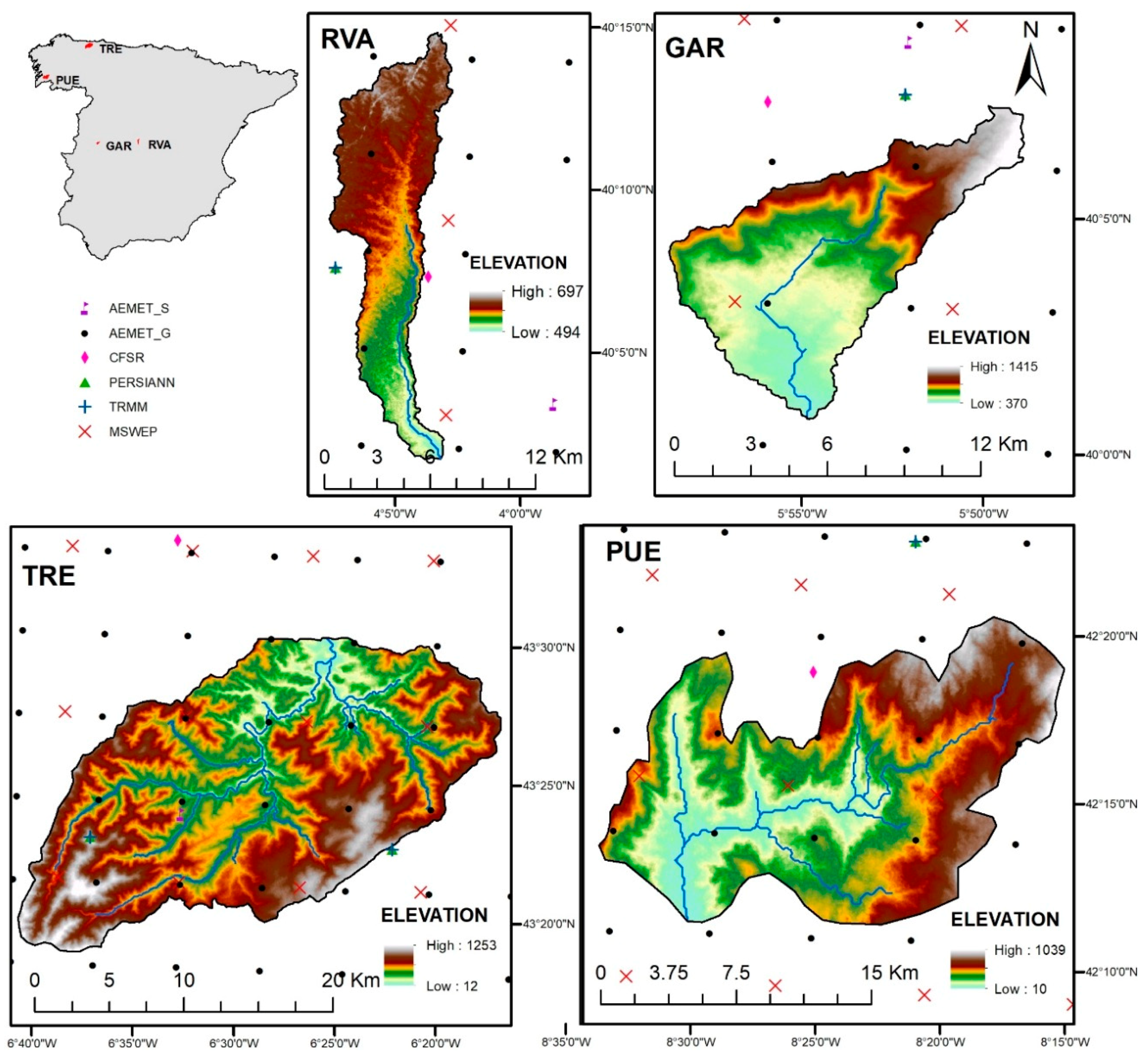
2.1. Study Area

Peninsular Spain features a wide range of climates, due to its position between the subtropical zone and the European temperate zone. It also includes some of the driest areas in the southeast, with a marked summer drought, and the rainiest areas in Europe in the northeast [24]. Four basins distributed over Peninsular Spain were used as study areas. The basins were selected based on the wide diversity of climate conditions representative of the types of weather found in Peninsular Spain. In addition, they are located in areas in which withdrawals are negligible and located upstream from reservoirs. As can be seen in Figure 1, the basins studied are well distributed over Peninsular Spain and represent four different climatic zones, according to the Köppen-Geiger classification system [36]. Table 1 shows basin sizes ranging from 70 km2 to 414 km2 and elevations ranging from 400 to 690 m. The average precipitation shown in Table 1 is from gauge measurements.

2.2. Datasets

In the following section, the gridded datasets used in this study are briefly introduced. All of the simulations were performed with monthly precipitation data, as well as monthly potential ETP and discharge time series for the common period (1998–2009) for all datasets (Table 2). The horizontal resolution of the gridded datasets used varied from 1 km grid to 0.3° × 0.3° spacing. The areal precipitation was estimated using Thiessen polygons. Even if this method does not take into account orography influences, it has been considered adequate in the present study due to the density of the spatial resolution of the datasets used. All of the MWBMs use rainfall and ETP time series as input data. The ETP data series in each basin were obtained from the official monthly series provided by the Centre of Studies and Experimentation of Civil Works (CEDEX) [37].

2.2.1. TRMM Dataset

The TRMM Multisatellite Precipitation Analysis (TMPA) provides a calibration-based sequential scheme for combining precipitation estimates from multiple satellites, as well as gauge analysis where feasible, at fine scales (0.25° × 0.25° and 3-hourly). The dataset covers the latitude band 50°N–S for the period from 1998 to the delayed present. The monthly product TRMM 3B43 was used in this study. More information about this dataset can be found in [11,14].

2.2.2. CFSR Dataset

The Climate Forecast System Reanalysis (CFSR) is a global coupled atmosphere-ocean-land surface-sea ice system and forecast model. The CFSR is based on hourly forecasts generated using information from satellite-derived products and the global weather station network, covering any location in the world [38]. The CFSR data have a spatial resolution of approximately 38 km, and the data are available from 1979 to present on the SWAT website. More information about this dataset can be found in [15].

2.2.3. PERSIANN Dataset

The PERSIANN-Climate Data Record (CDR) provides daily rainfall estimates at 0.25° spatial resolution for the latitude band 60°N–60°S over the period of 1983 to the delayed present. PERSIANN-CDR is generated from the PERSIANN algorithm, using infrared brightness temperature data from geostationary satellites to estimate rainfall rate and updating its parameters using passive/active microwave observations from low-orbital satellites. More information about this dataset can be found in [12].

2.2.4. MSWEP Dataset

The MSWEP version 2.1 is a fully global precipitation dataset for the period 1979 to 2016 with a 3-hourly temporal and 0.1° spatial resolution, specifically designed for hydrological modelling. MSWEP uses the complementary strengths of gauge-based, satellite-based, and reanalysis-based data to provide precipitation estimates over the entire globe. More information can be found in [13].

2.2.5. AEMET Dataset

The Spanish National Meteorological Agency (AEMET) grid, version 1.0, provides daily rainfall for the period of 1951 to the delayed present over Spain, with a spatial resolution of 5 km (AEMET_G). The method used is gauge analysis via Optimal Interpolation from the series of observations of the National Weather Data Bank of AEMET. More information about this dataset can be found in [39].

2.2.6. Rain Gauge Data

The gauged precipitation dataset consists of the nearest rain gauge records (AEMET_S) to each studied watershed (Figure 1), provided by the AEMET. The main characteristics of gauged stations are shown in Table 3.

3. Materials and Methods

3.1. Monthly Water Balance Models

Six well-known and documented MWBMs were used in this study: ABCD, AWBM, GR2M, Guo 5P, Thornthwaite, Mather, and Témez models. All these models are lumped and use a low number of parameters (from 2 to 5). The water balance in these models is represented by different storages, the moisture content of which varies depending on physical or empirical relationships [40]. More information about these MWBMs can be found in [24]. A brief description of the models is given below:
  • Thornthwaite-Mather (THM): It was developed in the early 1940s for the Delaware River, and several MWBMs are based on it. Based on the study of the model done by Alley [41], this model has two parameters (storage constant and soil moisture capacity) and two storages.
  • ABCD: It is composed of two storages. It is characterised by allowing streamflow to occur even under conditions of moisture deficit [42]. It has four parameters and emerges as a tool for assessment of water resources in the United States.
  • AWBM: It uses three storages to simulate partial surface run-off areas. The water balance in each of these storages is determined separately, using a total of six parameters [27]. It was developed in the 90s and today is one of the most widely used in Australia.
  • GR2M: It is an evolution of the GR2 model that provides a simplified representation of the rainfall/runoff process. It is characterised by a small number of parameters, developed with empirical criteria, which do not correspond to specific physical attributes. This model is composed of four parameters and two storages. The model has been tested in numerous French stations. The description of this MWBM can be found in the work of Makhlouf and Michel [43].
  • Guo: Described in [31,32], this MWBM is an adaptation of the model of Thornthwaite and Mather [44], increasing the number of parameters up to five. It has been applied in different sub-basins of the Dongjiang, in southern China, with good results. Xiong and Guo [31] compare it with the two-parameter model, concluding similar behaviour in practice.
  • Témez (TEM): It is a purely empirical model that has been widely used in many Spanish basins, especially for assessment of water resources developed by the Hydrographical Study Centre. The model considers the land to be divided into two zones: Upper unsaturated, or soil moisture, and lower saturated, or aquifer, which functions as an underground reservoir that drains into the network of channels [45]. This model uses four parameters. It is a lumped model that has been applied in a distributed way in order to obtain an evaluation of the Spanish water resources [46].

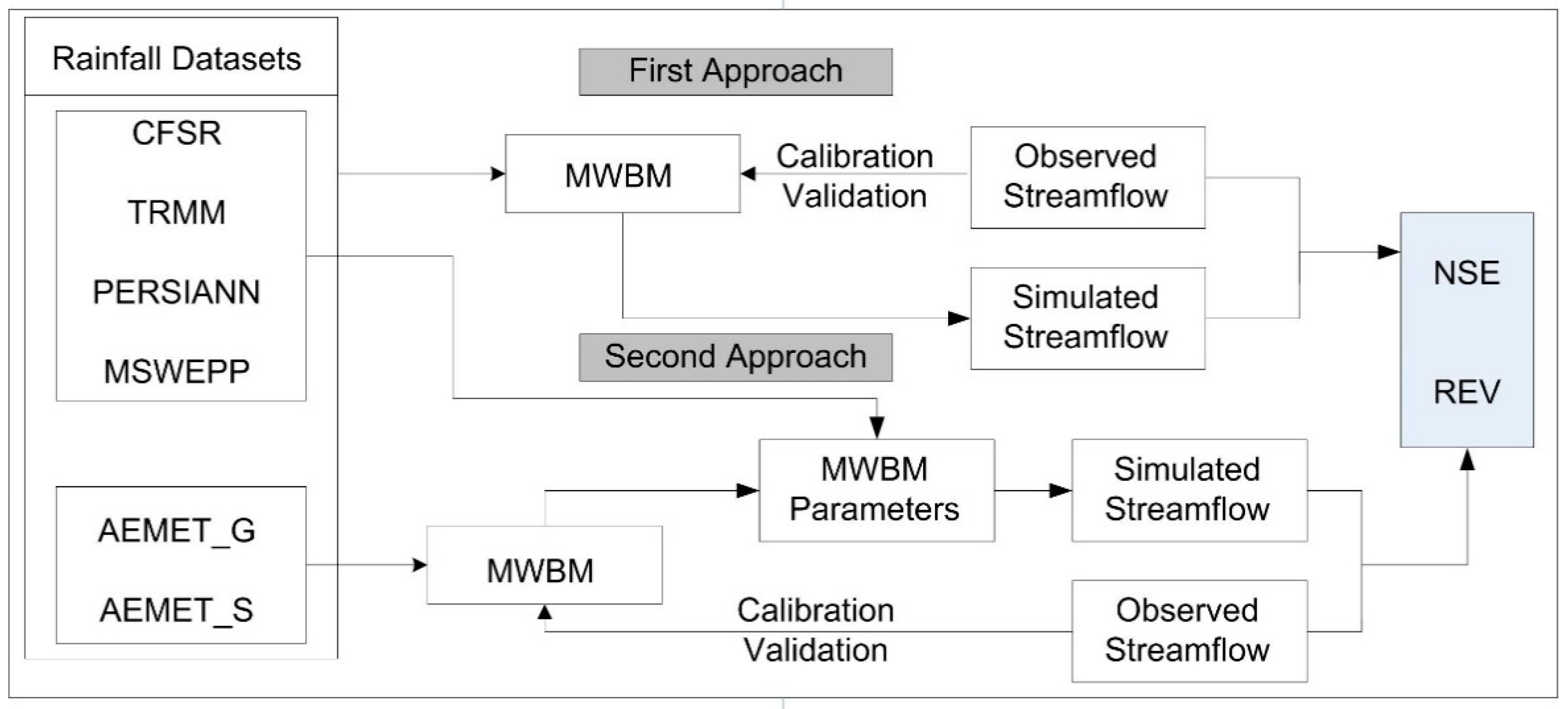
3.2. MWBM Calibration and Validation Strategy

The calibration of the MWBM parameters was carried out by comparing predicted data with observed data for a period of seven years (2003–2009). This period of time was chosen because it includes dry, average, and wet years, which is desirable to reach a good model calibration [47]. Monthly streamflow data were collected from the national water agency of Spain [37]. The value that minimizes the differences between both flow series and the objective function that minimizes the sum of square of deviations (SSQ) were considered the optimal values for each parameter. The optimization algorithm is the generalized reduced gradient (GRG2) [48], which searches for the extreme values of the functions by the GRG2 algorithm method [49]. During the calibration process of MWBMs, it was necessary to consider some initial conditions, such as the value of the initial soil moisture. These initial conditions tend to influence the final results; therefore, an initial period of two years (1998–1999) was used for model warm-up. After calibration, MWBMs were validated using the monthly discharge data of three years (2000–2002).

3.3. Performance of GPDs in Simulating Streamflow

There are two different strategies to assess the performance of the GPDs in simulating streamflow [50]. The first approach is calibration and validation of MWBMs using rain gauge data or gridded rainfall datasets with monthly observed streamflow. The second approach is calibration and validation of MWBMs with rain gauge data followed by the best fitted parameters found in MWBMs being used to simulate streamflow with GPDs. Artan et al. [51] and Zeweldi et al. [52] indicated that an MWBM can be improved when using satellite-based data [51,52,53]. Nevertheless, Habib et al. [54] considered that calibration achieved with GPDs could result in unrealistic parameter values in MWBMs to compensate for the large errors in input datasets. In this study, both approaches will be carried out (Figure 2).

3.4. Statistical Analysis

To quantitatively compare GPDs with rain gauge observations, widely used validation statistical indices are used in this study. The correlation coefficient (R) reflects the degree of linear correlation between GPDs and gauge observations, the relative bias (BIAS) is used to measure the systematic bias of the GPDs and the root mean square error (RMSE) quantifies the average error magnitude, which is slightly biased towards larger errors. R values vary from −1 to 1, with values closer to 1 indicating a positive correlation and high model performance. BIAS and RMSE values of 0 indicate a perfect fit.
R = i = 1 n ( G i   G ¯ ) ( S i   S ¯ ) i = 1 n ( G i   G ¯ ) 2 i = 1 n ( S i   S ¯ ) 2
BIAS = i = 1 n ( S i G i ) i = 1 n G i × 100 %
RMSE = 1 n i = 1 n ( S i G i ) 2
where S i is the precipitation from the rain gauge grid (AEMET_G), S ¯ is the average precipitation from the rain gauge grid, G i is the precipitation from GPDs, and G ¯ is the average precipitation from GPDs. In order to make a comparison among various MWBMs, some quantitative information is also required to measure model performance. In this study, the streamflow data measured at the outlet of the catchment was used to assess the model performance. Statistical performance indices, such as the Nash-Sutcliffe efficiency (NSE) [55] or the percentage difference between the total observed and modelled runoff (REV), have been calculated. NSE can range from −∞ to 1, with NSE = 1 being the optimal value. The REV optimal value is 0.
NSE = 1 i = 1 n ( O i M i ) 2 i = 1 n ( O i   O ¯ ) 2
REV = M T O T O T × 100 %
where O i is the observed discharge, M i is the modelled discharge, O ¯ is the mean of observed discharge, M T is the total modelled run-off, and O T is the total observed run-off.

4. Results

4.1. Comparison of Areal Mean Rainfalls

The first study performed consisted of analysing and comparing the areal mean rainfalls in the studied watersheds for the five different datasets considered. Figure 3 shows the accumulated precipitation from 1998 to 2009. As expected, both values of the national grid (AEMET_G) and the nearest rain gauge (AEMET_S) are quite similar, and their disparities in the last third of the period varies depending on the difference between rain gauge elevation, the watershed’s average altitude, and their proximity to the studied watershed. Thus, for example, TRE’s nearest record station is located in this watershed and within the average range of its altitude, so the accumulated precipitation only differs slightly. However, RVA’s rain gauge, which is located out of the boundaries of the watershed, is at a lower height than the whole study area and shows higher differences than the AEMET grid.
The long-term monthly areal rainfall for all the datasets considered and the four watersheds under study are shown in Figure 4. Although the monthly tendencies in all GPDs are similar to gauged data, the differences are mostly concentrated in the rainy seasons, while they are reduced in summer months. TRMM estimates are close to those from the rain gauge data and are lower than recorded precipitation, except in RVA, where MSWEP appears to be the dataset that fits the best with national grid or nearest rain gauges. Moreover, as in the accumulated precipitation analysis, GAR and RVA show the highest differences with GPDs, even wider in RVA, where TRMM and PERSIANN precipitation data are around 50% higher than the data from the AEMET dataset.
Previous findings are also confirmed with statistical analysis shown in Table 4, comparing the AEMET grid with the rest of the datasets. R values are no lower than 0.83, and, in most cases, higher than 0.95, which indicates a good lineal correlation, as can be seen in Figure 2 and Figure 3.
Concerning RMSE results, TRMM appears to be the best GPD in two out of the four watersheds (TRE and GAR), while MSWEP shows better results in PUE and RVA. However, the difference of RMSE values in PUE for TRMM and MSWEP only varies by 0.3 mm, so both GPDs could be used in similar regions to the studied ones according this goodness-of-fit test. Furthermore, PERSIANN reaches the worst values for nearly all the watersheds, until it doubles the lowest result.
BIAS results are less clear than RMSE ones, especially for the higher values. In all the watersheds, rain gauges show percentages lower than 10%, in some cases the lowest of the analysed values. TRMM also results in a good dataset for all watersheds, except the semi-arid one (RVA), where MSWEP presents, along with the nearest rain gauge, the best data according to BIAS values. However, PERSIANN was not found to be the worst dataset, as RMSE showed; it showed the best BIAS value (−0.27% in TRE) for all the possible combinations of watershed datasets studied. Notwithstanding, the drier the region is, the worse the value for PBIAS shows when using the PERSIANN grid.

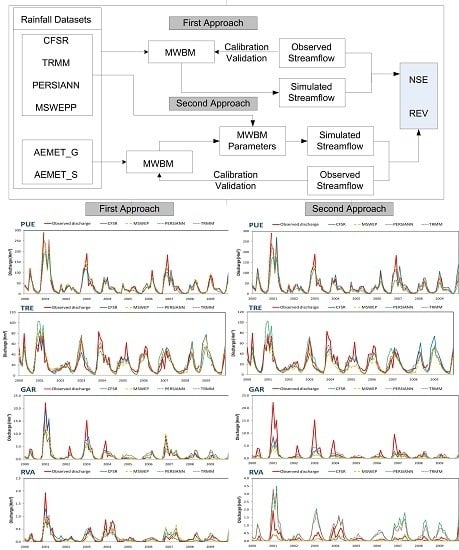
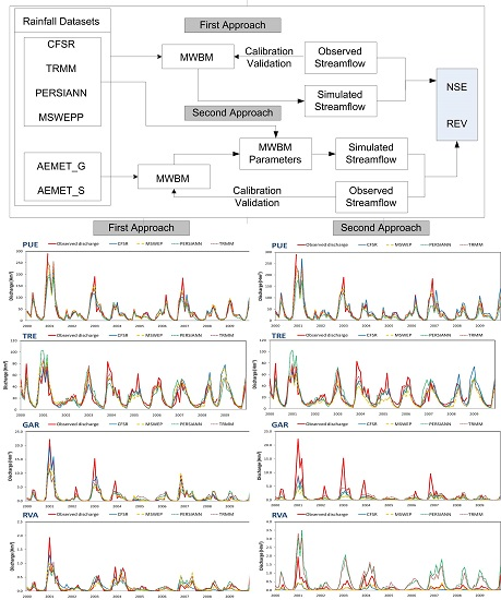
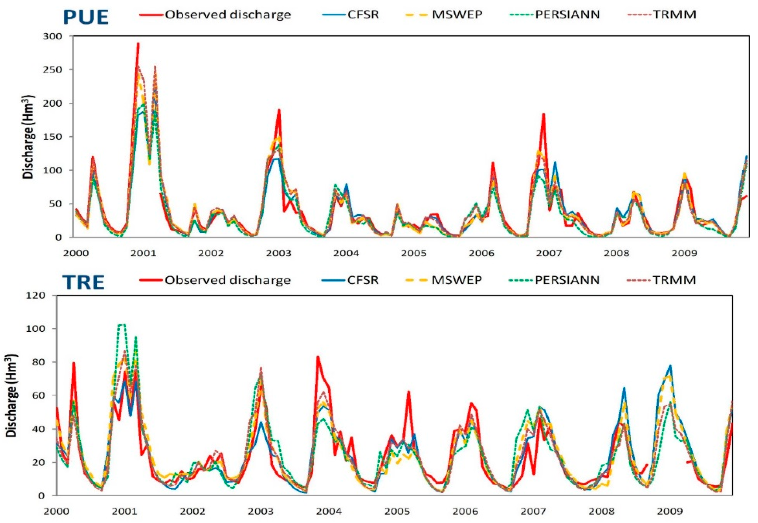
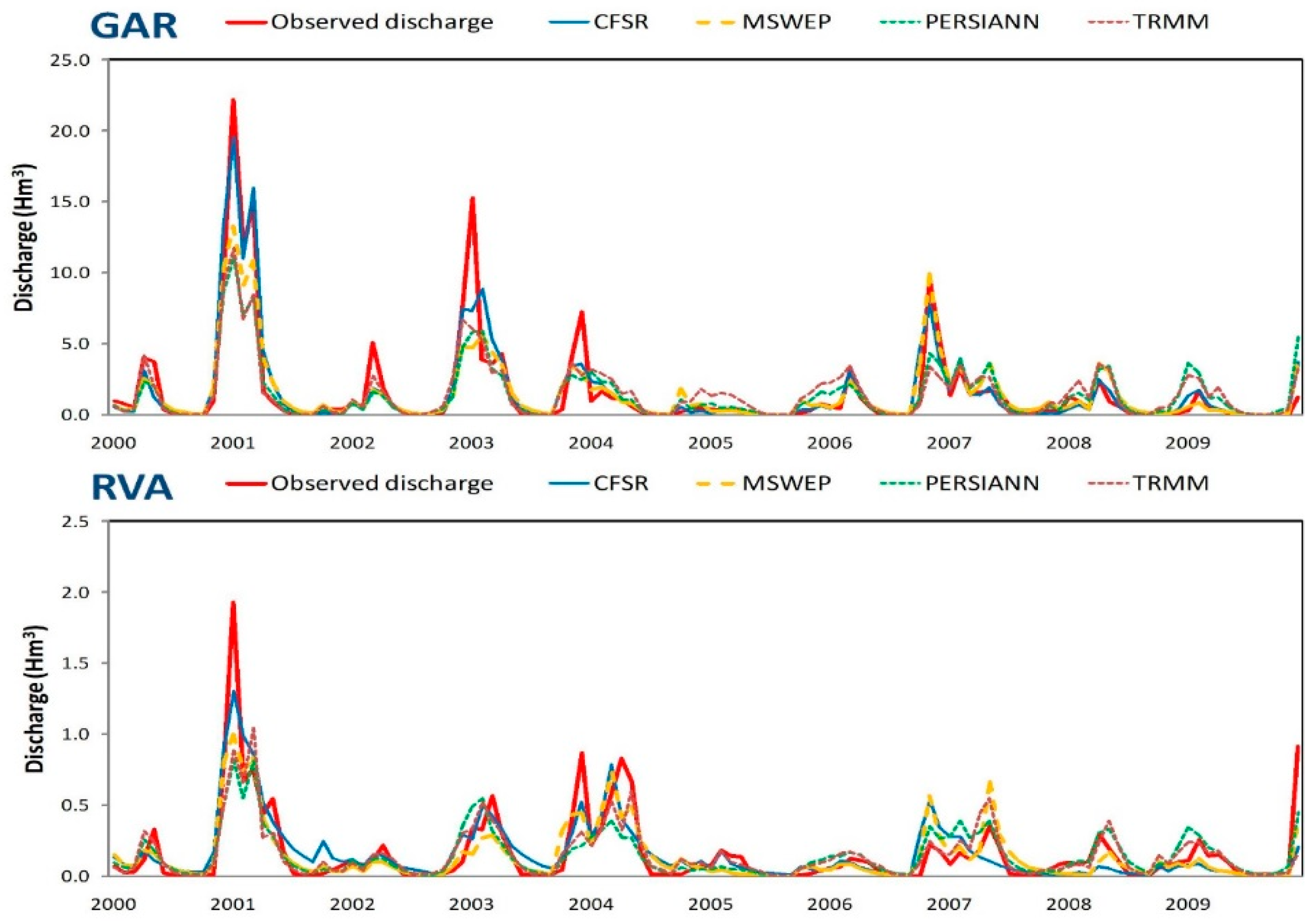
4.2. Evaluation of the Simulated Streamflow Using MWBM

The second phase of the research assessed the performance of the four GPDs and the two rain gauges’ banks of data from the AEMET (nearest one and grid) as input into the MWBMs considered for streamflow simulation in the four studied watersheds. Table 5 lists the NSE values when comparing observed and modelled streamflow for the best performance of each of the MWBMs, with every dataset taken into account. Furthermore, means have been calculated in each watershed, both for MWBMs and GPDs. The AEMET grid showed the best results, both mean and individual, for all the watersheds, while the nearest rain gauge only performed similarly to the grid in PUE and TRE; however, the NSE in GAR and RVA was not as satisfactory as the AEMET grid, although similar values to GPDs were achieved in most cases. The NSE mean in GR2M reached a value over 0.75 for the four watersheds, achieving its best value (0.95) in PUE for the AEMET_S, AEMET_G, and TRMM data. The rest of the models showed different values depending on the watershed. Thus, in PUE, all models except GR2M reached a similar NSE, around 0.64, 30% lower than GR2M. TRE did not vary more than 5%, regardless of the model used. These differences are slightly higher in GAR and reach more than 50% in RVA when comparing GR2M with ABCD or THM.
When comparing total volumes observed and modelled (Table 6) with REV, previous findings were confirmed. GR2M appeared to be the best model for all the watersheds [24], and, although AEMET_G did not give the lowest percentage in all cases, the difference was never over 5% compared with the rest of the datasets. TRMM and MSWEP results for GR2M were below 15% in all watersheds, except in GAR, where CFSR volume error was −1.59%, 20% lower than the others. CFSR also performed very satisfactorily in TRE and GAR, achieving a total streamflow error, compared to the observed, lower than 3.5% in GR2M, even better than in the AEMET datasets. PERSIANN appears to be the worst GPD in most cases, although greater value is shown with CFSR in RVA for THM, doubling the observed streamflow in this watershed. No trend was found related to over- or underestimating total streamflow when using this goodness-of-fit measure.

4.3. Evaluation of GPDs Using the AEMET_G-Calibrated GR2M

Given the large number of parameters that were forced, in calibration analysis, to the extreme values range of MWBMs with satellite precipitation datasets, a ‘second approach’ was applied. Thus, once it was demonstrated that the AEMET grid is the best dataset for all watersheds and that GR2M shows, on average, the best performance in the different climate regions in Peninsular Spain, experiments based on the well-calibrated model were conducted to evaluate streamflow predictions with input from rain gauge data and the four gridded rainfall datasets over the four watersheds. All watersheds reached the best result with the nearest rain gauge for both NSE and REV (Table 7). TRMM showed the best performance in three out of the four watersheds among the GPDs studied, because RVA does not exceed 0.33 NSE with MSWEP, and the lowest REV is over 60%, although the rest of the GPDs showed worse errors. There is, once again, a clear trend towards worse performance the drier the watershed is, substantially decreasing in NSE value from an average 0.82 in PUE to negative values in RVA. REV results indicated higher variation depending on the GPD, but this also followed same tendency of increasing errors the drier the watershed is. Despite these wide ranges in REV, an underestimation of streamflow in GPDs was confirmed, becoming near −80% in GAR, even if in RVA this trend was reversed with TRMM and PERSIANN. The latter reached the worst results for the four watersheds, except for GAR.

5. Discussion

The use of point-scale gauge records can lead to important deviations in areal precipitations, as suggested by Tang et al. [4], especially the drier the watershed is. With regard to GPDs, as has been reported by other authors [56,57], the volumes of precipitation of the satellite precipitation products tended to be smaller than those of the gauged data in most cases, and these differences are greater the drier the watershed is, as in the cases of GAR and RVA. MSWEP and PERSIANN show the highest differences in accumulated precipitation, normally lower, except for the semi-arid watershed (RVA). Furthermore, even in RVA, PERSIANN and TRMM datasets show volumes higher than gauged records.
Concerning the goodness-of-fit tests, R does not seem to be a good measure to assess the validity of the studied datasets, because the results did not differ much from the others [58]. In fact, when using other criteria, both graphical and metrics, the performance of the datasets are clearly different.
The results confirmed that TRMM and CFSR are, on average, the models that reached the best performance in all the watersheds, with slight differences that are higher the drier the watershed is. The good performance of TRMM is also shown in other recent studies that used TRMM datasets worldwide [59,60]. However, the good results achieved with PERSIANN grid in [8] are not found in the present study, due to various and extreme climatic conditions which characterize Spain, as in the case of complex topography in Chile shown by Zambrano-Bigiarini et al. [61].
Regarding the MWBMs, GR2M gave the best results in all the watersheds for most of the rainfall products used, as previously reported by Pérez-Sánchez et al. [24] in Peninsular Spain. On the contrary, ABCD or THM may be considered the ones with the worst performance in a semi-arid watershed, but did not show such unsatisfactory results in the rest of the climate watersheds studied. The commonly used model in Spain, TEM, gave poor results (25% on average). In general, worse performance of MWBMs was observed the drier the watershed climate was. Because the gauge network density is similar in both the wet and dry regions, the uneven distribution of precipitation in semi-arid watersheds seems to be the reason why the performance of the datasets and models is very different.
Figure 5 shows the comparison between the observed and simulated streamflow when using GR2M, which resulted, as seen, generally, in the best MWBM in the four watersheds. The peaks of simulated flow are poorly modelled due to the underestimation in precipitation driven by the GPDs. These differences tend to be higher the drier the watershed is, as shown before, and regardless of the area. In fact, PUE and TRE observed peaks in the rainiest years (2001, 2003, and 2007) are nearer to simulated ones with most GPDs (especially TRMM and MSWEP) than in GAR and RVA watersheds, where simulated peak flows in 2001, 2003, and 2004 are lower than observed ones [62,63,64]. Nevertheless, there are other peak flows (though lesser in number) where simulated peak flows exceed observed ones, such as PERSIANN in TRE in 2001 and MSWEP and PERSIANN in RVA in 2007 and 2008, highlighting the higher precipitation volumes in these GPDs. However, base flows are well-modelled in all watersheds, reflecting the good results in NSE with GR2M (Table 4), despite differences in peaks, which are reflected in REV (Table 6).
When using the second approach (Figure 6), whilst TRMM and MSWEP performed similarly both in base and peak flows in the more humid watershed (PUE), errors in peak flows were higher the more arid the watershed was. Although TRMM-simulated peak flows in the 2004–2006 period are lower than observed ones in TRE, total volume difference in the study period represents less than 10%. The CFSR dataset exhibited similar behaviour to TRMM, except in the last three years, where peak flows were higher than observed ones, as with PERSIANN in 2001. On the contrary, differences with MSWEP became even larger from 2002 in TRE, and streamflow was underestimated both in GAR and RVA, as with CFSR. None of the GPDs gave satisfactory results in this approach in the semi-arid watershed (RVA), overestimating total volume by up to 200% with TRMM and PERSIANN, and underestimating it by around 65% with CFSR and MSWEP.

6. Conclusions

In this study, satellite rainfall products represented by PERSIANN, TRMM, CSFR, and MSWEP were assessed for the quality of their rainfall estimates on a monthly scale based on data from ground observations over four basins located in Peninsular Spain, which cover different climatic zones, for the period of January 2000 to December 2009. Due to the uniform coverage and no missing data, gridded datasets are much easier to use than station data. The following conclusions can be drawn from the results of this study:
  • The results underscore the superiority of the national gridded dataset over the other rainfall remote sensing products examined in this study.
  • The use of point-scale gauge records can lead to important deviations in areal precipitations, especially the drier the watershed is.
  • The better estimation of volumes of precipitation by using MSWEP would possibly be due to its finer resolution. However, that is not altogether necessary for success in better streamflow forecast.
  • The precipitation volumes of the GPDs tend to be smaller than those of the gauged data. However, PERSIANN and TRMM datasets show volumes higher than gauged records in semi-arid watersheds.
  • The lumped GR2M model provides a better streamflow forecast than the other MWBMs in Peninsular Spain watersheds. Notwithstanding, the performance of GPDs and MWBMs highly depends on the climate: The more humid the watershed is, the better results can be achieved.
  • When using GPDs in MWBM parameter calibration, TRMM rainfall data provides the best performance in simulating streamflow, with satisfactory precision in all watersheds according to NSE. However, CFSR achieves better results with regard to total volume recorded in sub-humid watersheds.
  • Calibration achieved directly with GPDs could result in unrealistic parameter values in MWBMs to compensate for the large errors in input datasets. Thus, an assessment of previously fitted value parameters should be taken in account. Likewise, a study of MWBM performance and best fitted parameters with rain gauge data should be used with GPDs, in order to avoid invalid or extreme parameter values in MWBMs.
  • When using rain gauge grid dataset-fitted parameters in MWBMs, TRMM was also the best GPD in humid and sub-humid watersheds, but its performance loses effectiveness the more arid the watershed is, as the rest of the GPDs showed, especially in peak flows, due to both the underestimation and overestimation of the extreme gauge precipitation in semi-arid watersheds.
  • The uneven distribution of precipitation in semi-arid watersheds seems to be the reason why the performance of datasets and models is worse than in humid and sub-humid regions.
  • Because semi-arid watersheds do not seem to provide very good results with the MWBMs and GPDs used, and because satellite rainfall datasets continue to improve, further analysis with other satellite data products and the joint use of (semi-) distributed models and downscaling datasets [65] are recommended for future studies, according to the methodology followed in developing this study. Likewise, sequential data assimilation techniques [66] may improve current hydrology model outputs using real-time observations.
The procedures used can be applied in regions with similar case studies to more accurately assess the resources within a system in which there is scarcity of recorded data available.

Author Contributions

J.S.-A. and J.P.-S. conceived and designed the experiments; A.L.-B. and F.J.S.-M. performed the experiments and analysed the data; D.P.-V. provided reviews and suggestions; J.P.-S. and J.S.-A. prepared the manuscript with contributions from all co-authors.

Acknowledgments

This research has been partially supported by the Euro-Mediterranean Water Institute (Grant No. 57/15). In addition, the authors acknowledge Papercheck Proofreading & Editing Services.

Conflicts of Interest

The authors declare no conflicts of interest.

References

  1. Sun, Q.; Miao, C.; Duan, Q.; Ashouri, H.; Sorooshian, S.; Hsu, K.-L. A review of global precipitation data sets: Data sources, estimation, and intercomparisons. Rev. Geophys. 2018, 56. [Google Scholar] [CrossRef]
  2. Liu, X.; Yang, T.; Hsu, K.; Liu, C.; Sorooshian, S. Evaluating the streamflow simulation capability of PERSIANN-CDR daily rainfall products in two river basins on the Tibetan Plateau. Hydrol. Earth Syst. Sci. 2017, 21, 169–181. [Google Scholar] [CrossRef] [Green Version]
  3. Infante-Corona, J.A.; Lakhankar, T.; Pradhanang, S.; Khanbilvardi, R. Remote Sensing and Ground-Based Weather Forcing Data Analysis for Streamflow Simulation. Hydrology 2014, 1, 89–111. [Google Scholar] [CrossRef] [Green Version]
  4. Tang, G.; Behrangi, A.; Long, D.; Li, C.; Hong, Y. Accounting for spatiotemporal errors of gauges: A critical step to evaluate gridded precipitation products. J. Hydrol. 2018, 559. [Google Scholar] [CrossRef]
  5. Villarini, G.; Mandapaka, P.; Krajewski, V.; Witold, F.; Moore, R. Rainfall and sampling uncertainties: A rain gauge perspective. J. Geophys. Res. Atmos. 2008. [Google Scholar] [CrossRef]
  6. Jensen, N.E.; Pedersen, L. Spatial Variability of Rainfall. Variations within a Single Radar Pixel. J. Atmos. Res. 2005, 77, 269–277. [Google Scholar] [CrossRef]
  7. Wood, S.J.; Jones, D.A.; Moore, R. Accuracy of rainfall measurement for scales of hydrological interest. Hydrol. Earth Syst. Sci. 2000, 4, 531–543. [Google Scholar] [CrossRef] [Green Version]
  8. Tan, M.L.; Gassman, P.W.; Cracknell, A.P. Assessment of Three Long-Term Gridded Climate Products for Hydro-Climatic Simulations in Tropical River Basins. Water 2017, 9, 229. [Google Scholar] [CrossRef]
  9. Faramarzi, M.; Srinivasan, R.; Iravani, M.; Bladon, K.D.; Abbaspour, K.C.; Zehnder, A.J.B.; Goss, G.G. Setting up a hydrological model of Alberta: Data discrimination analyses prior to calibration. Environ. Model. Softw. 2015, 74, 48–65. [Google Scholar] [CrossRef]
  10. Raimonet, M.; Oudin, L.; Thieu, V.; Silvestre, M.; Vautard, R.; Rabouille, C.; Le Moigne, P. Evaluation of Gridded Meteorological Datasets for Hydrological Modeling. J. Hydrometeorol. 2017, 18, 3027–3041. [Google Scholar] [CrossRef]
  11. Huffman, G.J.; Bolvin, D.T.; Nelkin, E.J.; Wolff, D.B.; Adler, R.F.; Gu, G.; Stocker, E.F. The TRMM Multisatellite Precipitation Analysis (TMPA): Quasi-global, multiyear, combined-sensor precipitation estimates at fine scales. J. Hydrometeorol. 2007, 8, 38–55. [Google Scholar] [CrossRef]
  12. Ashouri, H.; Hsu, K.-L.; Sorooshian, S.; Braithwaite, D.K.; Knapp, K.R.; Cecil, L.D.; Prat, O.P. PERSIANN-CDR: Daily precipitation climate data record from multi-satellite observations for hydrological and climate studies. Bull. Am. Meteorol. Soc. 2015, 96, 69–83. [Google Scholar] [CrossRef]
  13. Beck, H.E.; van Dijk, A.I.J.M.; Levizzani, V.; Schellekens, J.; Miralles, D.G.; Martens, B.; de Roo, A. MSWEP: 3-hourly 0.25° global gridded precipitation (1979–2015) by merging gauge, satellite, and reanalysis data. Hydrol. Earth Syst. Sci. 2017, 21, 589–615. [Google Scholar] [CrossRef] [Green Version]
  14. Beck, H.E.; Vergopolan, N.; Pan, M.; Levizzani, V.; van Dijk, A.I.J.M.; Weedon, G.P.; Brocca, L.; Pappenberger, F.; Huffman, G.J.; Wood, E.F. Global-scale evaluation of 22 precipitation datasets using gauge observations and hydrological modeling. Hydrol. Earth Syst. Sci. 2017, 21, 6201–6217. [Google Scholar] [CrossRef] [Green Version]
  15. Saha, S.; Moorthi, S.; Wu, X.; Wang, J.; Nadiga, S.; Tripp, P.; Behringer, D.; Hou, Y.T.; Chuang, H.Y.; Iredell, M. The NCEP climate forecast system version 2. J. Clim. 2014, 27, 2185–2208. [Google Scholar] [CrossRef]
  16. Hyun-Goo, K.; Jin-Young, K.; Yong-Heack, K. Comparative Evaluation of the Third-Generation Reanalysis Data for Wind Resource Assessment of the Southwestern Offshore in South Korea. Atmosphere 2018, 9, 73. [Google Scholar] [CrossRef]
  17. Yang, Y.; Wang, G.; Wang, L.; Yu, J.; Xu, Z. Evaluation of Gridded Precipitation Data for Driving SWAT Model in Area Upstream of Three Gorges Reservoir. PLoS ONE 2014, 9, 11. [Google Scholar] [CrossRef] [PubMed]
  18. Xu, H.; Xu, C.Y.; Sælthun, N.R.; Zhou, B.; Xu, Y. Evaluation of reanalysis and satellite-based precipitation datasets in driving hydrological models in a humid region of southern China. Stoch. Environ. Res. Risk Assess. 2015, 29, 2003–2020. [Google Scholar] [CrossRef]
  19. Dos Reis, J.B.C.; Rennó, C.D.; Lopes, E.S.S. Validation of Satellite Rainfall Products over a Mountainous Watershed in a Humid Subtropical Climate Region of Brazil. Remote Sens. 2017, 9, 1240. [Google Scholar] [CrossRef]
  20. Seneviratne, S.I.; Corti, T.; Davin, E.L.; Hirschi, M.; Jaeger, E.B.; Lehner, I.; Orlowsky, B.; Teuling, A.J. Investigating soil moisture–climate interactions in a changing climate: A review. Earth Sci. Rev. 2010, 99, 125–161. [Google Scholar] [CrossRef]
  21. Hafeez, M.; van de Giesen, N.; Bardsley, E.; Seyler, F.; Pail, R.; Taniguchi, M. GRACE, Remote Sensing and Ground-Based Methods in Multi-Scale Hydrology: Proceedings of Symposium JHO1 Held during IUGG2011; IAHS Publications: Boulder, CO, USA, 2011; ISBN 978-1-907161-18-6. [Google Scholar]
  22. Wurbs, R.A. Texas water availability modeling system. J. Water Resour. Plan. Manag. 2005, 131, 270–279. [Google Scholar] [CrossRef]
  23. Sitterson, J.; Knightes, C.; Parmar, R.; Wolfe, K.; Muche, M.; Avant, B. An Overview of Rainfall-Runoff Model Types. EPA 2017 Office of Research and Development (8101R) Washington, DC 20460. Available online: https://cfpub.epa.gov/si/si_public_file_download.cfm?p_download_id=533906 (accessed on 5 June 2018).
  24. Pérez-Sánchez, J.; Senent-Aparicio, J.; Segura-Méndez, F.; Pulido-Velázquez, D. Assessment of lumped hydrological balance models in Peninsular Spain. Hydrol. Earth Syst. Sci. Discuss. 2017, 424. [Google Scholar] [CrossRef]
  25. Marinou, P.G.; Feloni, E.G.; Tzoraki, O.; Baltas, E.A. An implementation of a water balance model in the Evrotas basin. EWRA 2017, 57, 147–154. [Google Scholar]
  26. Wriedt, G.; Bouraoui, F. Towards a General Water Balance Assessment of Europe; Joint Research Centre—Institute for Environment and Sustainability; Office for Official Publications of the European Communities: Luxembourg, 2009. [Google Scholar]
  27. Boughton, W.C. The Australian water balance model. Environ. Model. Softw. 2004, 19, 943–956. [Google Scholar] [CrossRef]
  28. Zhang, Q.; Liu, J.; Singh, V.P.; Gu, X.; Chen, X. Evaluation of impacts of climate change and human activities on streamflow in the Poyang Lake basin, China. Hydrol. Process. 2016, 30, 2562–2576. [Google Scholar] [CrossRef]
  29. Sharifi, M.A.; Rodriguez, E. Design and development of a planning support system for policy formulation in water resources rehabilitation: The case of Alcázar De San Juan District in Aquifer 23, La Mancha, Spain. J. Hydroinform. 2002, 4, 157–175. [Google Scholar] [CrossRef]
  30. Barros, R.; Isidoro, D.; Aragüés, R. Long-term water balances in La Violada irrigation district (Spain): I. Sequential assessment and minimization of closing errors. Agric. Water Manag. 2011, 102, 35–45. [Google Scholar] [CrossRef] [Green Version]
  31. Xiong, L.; Guo, S. A two-parameter monthly water balance model and its application. J. Hydrol. 1999, 216, 111–123. [Google Scholar] [CrossRef]
  32. Guo, S. Impact of Climate Change on Hydrological Balance and Water Resource Systems in the Dongjiang Basin, China; Modeling and Management of Sustainable Basin-Scale Water Resource Systems (Proceedings of a Boulder Symposium; ed. by S. P. Simonovic, Z. W. Kundzewicz, D. Rosbjerg & K. Takeuchi); IAHS Publications: Boulder, CO, USA, 1995. [Google Scholar]
  33. Escriva-Bou, A.; Pulido-Velazquez, M.; Pulido-Velazquez, D. Economic value of climate change adaptation strategies for water management in Spain’s Jucar basin. J. Water Res. Plan. ASCE 2017, 143. [Google Scholar] [CrossRef]
  34. MIMAM. Libro Blanco del Agua en España; Centro de Publicaciones del Ministerio de Medio Ambiente: Madrid, Spain, 2000. [Google Scholar]
  35. Estrela, T. Modelos Matemáticos Para la Evaluación de Recursos Hídricos; Centro de Estudios Hidrográficos y Experimentación de Obras Públicas: Madrid, Spain, 1992. [Google Scholar]
  36. Kottek, M.; Grieser, J.; Beck, C.; Rudolf, B.; Rubel, F. World map of the Köppen-Geiger climate classification. Meteorol. Z. 2006, 15, 259–263. [Google Scholar] [CrossRef]
  37. CEDEX. 2018. Available online: http://www.cedex.es (accessed on 20 April 2018).
  38. Radcliffe, D.E.; Mukundan, R. PRISM vs. CFSR Precipitation Data Effects on Calibration and Validation of SWAT Models. JAWRA J. Am. Water Resour. Assoc. 2016, 1–12. [Google Scholar] [CrossRef]
  39. Peral García, C.; Navascués Fernández-Victorio, B.; Ramos Calzado, P. Serie de Precipitación Diaria en Rejilla con Fines Climáticos. Nota Técnica 24 de AEMET; Spanish Meteorological Agency (AEMET): Madrid, Spain, 2017. [Google Scholar]
  40. Xu, C.Y.; Singh, V.P. A review on monthly water balance models for water resources investigations. Hydrol. Process. 1998, 12, 31–50. [Google Scholar]
  41. Alley, W.M. On the treatment of Evapotranspiration, Soil Moisture Accounting and Aquifer Recharge in Monthly Water Balance Models. Water Resour. Res. 1984, 20, 1137–1149. [Google Scholar] [CrossRef]
  42. Thomas, H.A. Improved Methods for National Water Assessment; Report, contract: WR 15249270; U.S. Water Resources Council: Washington, DC, USA, 1981.
  43. Makhlouf, Z.; Michel, C. A two-parameter monthly water balance model for french watersheds. J. Hydrol. 1994, 162, 299–318. [Google Scholar] [CrossRef]
  44. Thornthwaite, C.W.; Mather, J.R. Instructions and Tables for Computing Potential Evapotranspiration and the Water Balance; Publications in Climatology, 10.3; Drexel Institute: Centerton, NJ, USA, 1957. [Google Scholar]
  45. Témez, J.R. Modelo Matemático de Transformación "Precipitación-Aportación"; Asociación de Investigación Industrial Eléctrica (ASINEL): Madrid, Spain, 1977. [Google Scholar]
  46. Estrela, T.; Cabezas, F.; Estrada, F. La evaluación de los recursos hídricos en el Libro Blanco del Agua en España. Ingeniería del Agua 1999, 6, 125–138. [Google Scholar] [CrossRef]
  47. Gan, T.Y.; Dlamini, E.M.; Biftu, G.F. Effects of model complexity and structure, data quality, and objective functions on hydrologic modeling. J. Hydrol. 1997, 192, 81–103. [Google Scholar] [CrossRef]
  48. Fylstra, D.; Lasdon, L.; Watson, J.; Waren, A. Design and use of the Microsoft Excel Solver. Interfaces 1998, 28, 29–55. [Google Scholar] [CrossRef]
  49. Lasdon, L.S.; Waren, A.D.; Jain, A.; Ratner, M. Design and testing of a generalized reduced gradient code for nonlinear programming. ACM Trans. Math. Softw. 1978, 4, 34–50. [Google Scholar] [CrossRef]
  50. Zeweldi, D.A.; Gebremichale, M.; Downer, C.W. On CMORPH rainfall for streamflow simulation in a small, Hortonian watershed. J. Hydrometeorol. 2011, 12, 456–466. [Google Scholar] [CrossRef]
  51. Artan, G.; Gadain, H.; Smith, J.L.; Asante, K.; Bandaragoda, C.J.; Verdin, J.P. Adequacy of satellite derived rainfall data for streamflow modelling. Nat. Hazards 2007, 43, 167–185. [Google Scholar] [CrossRef]
  52. Yilmaz, K.K.; Hogue, T.S.; Hsu, K.L.; Sorooshian, S.; Gupta, H.V.; Wagener, T. Intercomparison of rain gauge, radar, and satellite-based precipitation estimates with emphasis on hydrologic forecasting. J. Hydrometeorol. 2005, 6, 497–517. [Google Scholar] [CrossRef]
  53. Bitew, M.M.; Gebremichael, M.; Ghebremichael, L.T.; Bayissa, Y.A. Evaluation of high resolution satellite rainfall products through streamflow simulation in a hydrological modeling of a Small Mountainous Watershed in Ethiopia. J. Hydrometeorol. 2012, 13, 338–350. [Google Scholar] [CrossRef]
  54. Habib, E.; Haile, A.T.; Sazib, N.; Zhang, Y.; Rientjes, T. Effect of bias correction of satellite-rainfall estimates on runoff simulations at the source of the Upper Blue Nile. Remote Sens. 2014, 6, 6688–6708. [Google Scholar] [CrossRef]
  55. Nash, J.E.; Sutcliffe, J.V. River flow forecasting through conceptual models. Part I—A discussion of principles. J. Hydrol. 1970, 10, 282–290. [Google Scholar] [CrossRef]
  56. Sidike, A.; Chen, X.; Liu, T.; Durdiev, K.; Huang, Y. Investigating alternative climate data sources for hydrological simulations in the upstream of the Amu Darya River. Water 2016, 8, 441. [Google Scholar] [CrossRef]
  57. Yoshimoto, S.; Amarnath, G. Applications of Satellite-Based Rainfall Estimates in Flood Inundation Modeling—A Case Study in Mundeni Aru River Basin, Sri Lanka. Remote Sens. 2017, 9, 998. [Google Scholar] [CrossRef]
  58. Pérez-Sánchez, J.; Senent-Aparicio, J.; Díaz-Palmero, J.M.; Cabezas-Cerezo, J.D. A comparative study of fire weather indices in a semiarid south-eastern Europe region. Case of study: Murcia (Spain). Sci. Total Environ. 2017, 15, 590–591, 761–774. [Google Scholar] [CrossRef] [PubMed]
  59. Caparoci Nogueira, S.M.; Moreira, M.A.; Lordelo Volpato, M.M. Evaluating Precipitation Estimates from Eta, TRMM and CHRIPS Data in the South-Southeast Region of Minas Gerais State—Brazil. Remote Sens. 2018, 10, 313. [Google Scholar] [CrossRef]
  60. Cao, Y.; Zhang, W.; Wang, W. Evaluation of TRMM 3B43 data over the Yangtze River Delta of China. Sci. Rep. 2018, 8, 5290. [Google Scholar] [CrossRef] [PubMed] [Green Version]
  61. Zambrano-Bigiarini, M.; Nauditt, A.; Birkel, C.; Verbist, K.; Ribbe, L. Temporal and spatial evaluation of satellite-based rainfall estimates across the complex topographical and climatic gradients of Chile. Hydrol. Earth Syst. Sci. 2017, 21, 1295–1320. [Google Scholar] [CrossRef] [Green Version]
  62. Dinku, T.; Ceccato, P.; Grover-Kopec, E.; Lemma, M.; Connor, S.J.; Ropelewski, C.F. Validation of satellite rainfall products over East Africa’s complex topography. Int. J. Remote Sens. 2007, 28, 1503–1526. [Google Scholar] [CrossRef]
  63. Karaseva, M.O.; Prakash, S.; Gairola, R.M. Validation of high-resolution TRMM-3B43 precipitation product using rain gauge measurements over Kyrgyzstan. Theor. Appl. Climatol. 2012, 108, 147–157. [Google Scholar] [CrossRef]
  64. Guo, R.; Liu, Y. Evaluation of Satellite Precipitation Products with Rain Gauge Data at Different Scales: Implications for Hydrological Applications. Water 2016, 8, 281. [Google Scholar] [CrossRef]
  65. Omranian, E.; Sharif, H.O. Evaluation of the Global Precipitation Measurement (GPM) Satellite Rainfall Products over the Lower Colorado River Basin, Texas. J. Am. Water Resour. Assoc. 2018. [Google Scholar] [CrossRef]
  66. Javaheri, A.; Nabatian, M.; Omranian, E.; Babbar-Sebens, M.; Noh, S.J. Merging Real-Time Channel Sensor Networks with Continental-Scale Hydrologic Models: A Data Assimilation Approach for Improving Accuracy in Flood Depth Predictions. Hydrology 2018, 5, 9. [Google Scholar] [CrossRef]
Figure 1. Location, elevation, and gridded precipitation datasets of the selected basins.
Remotesensing 10 00922 g001
Figure 2. Flowchart for comparative study.
Remotesensing 10 00922 g002
Figure 3. Accumulated monthly precipitation over selected basins for ground observations and gridded precipitation datasets in the 1998–2009 period.
Remotesensing 10 00922 g003aRemotesensing 10 00922 g003b
Figure 4. Long-term monthly areal precipitation of ground observations and gridded precipitation products in the 1998–2009 period.
Remotesensing 10 00922 g004
Figure 5. Observed and simulated monthly flow hydrographs for the different datasets using GR2M during the calibration and validation periods (2000–2009).
Remotesensing 10 00922 g005aRemotesensing 10 00922 g005b
Figure 6. Observed and simulated monthly flow hydrographs for the different datasets using the AEMET_G-calibrated GR2M during the calibration and validation periods (2000–2009).
Remotesensing 10 00922 g006
Table 1. Summary of the main characteristics of the selected basins (1998–2009).
CodeArea (km2)Altitude (m.a.s.l)Average Slope (%)Köppen ClassificationAverage Precipitation (mm/year)Average ETP (mm)Average Flow (hm3/year)
RVA8660818.33Bsk42210342.2
GAR7069032.44Csa1081104018.9
PUE26440018.43Csb1624762435.2
TRE4145277.51Cfb1241674300.9
Table 2. List of datasets used in this study and coverage periods.
DatasetVersionSpatial ResolutionAreal CoverageTemporal ResolutionTemporal CoverageData SourcesSource
CFSRDS093.10.3° × 0. 3° (≈38 km)GlobalDaily1979–presentReanalysis[15]
TRMM3B430.25° × 0.25° (≈30 km)Latitude band 50°N–S3-hourly1998–presentGauge, satellite[11]
PERSIANNCDR0.25° × 0.25° (≈30 km)Latitude band 60°N–SDaily1983–presentGauge, satellite[12]
MSWEPV2.10.1° × 0.1° (≈12 km)Global3-hourly1979–2016Gauge, satellite, reanalysis[13]
AEMET_GV1.05 kmSpainDaily1951–2017Gauge[39]
Table 3. Rain gauge station characteristics used in the study.
Basin CodeStation NameLatitudeLongitudeAltitude (m.a.s.l)Source
RVARecas39.96−4.01609SIAR 1
GARValdastillas40.14−5.87495REDAREX 2
PUEVigo/Peinador42.24−8.62261AEMET 3
TREZardain43.39−6.55410AEMET
1 SIAR: Castilla-La Mancha Irrigation Consultancy Service; 2 REDAREX: Extremadura Irrigation Consultancy Service; 3 AEMET: Spanish National Meteorology Agency.
Table 4. Statistical indices used to quantify the accuracy of precipitation estimates against precipitation from AEMET_G (best results in bold).
BasinsDatasetRRMSE (mm)BIAS (%)
PUEAEMET_S0.9918.05−3.82
TRMM0.9918.582.53
PERSIANN0.9748.0117.94
CFSR0.9830.77−8.90
MSWEP0.9918.283.54
TREAEMET_S0.9913.02−2.46
TRMM0.9620.684.19
PERSIANN0.8339.34−0.27
CFSR0.9423.153.43
MSWEP0.9430.0516.56
GARAEMET_S0.9625.716.02
TRMM0.9541.1914.88
PERSIANN0.9555.7332.00
CFSR0.9553.6540.39
MSWEP0.9463.4346.04
RVAAEMET_S0.9312.5110.06
TRMM0.9522.28−50.29
PERSIANN0.9125.97−56.53
CFSR0.8821.3438.88
MSWEP0.9413.9822.75
Table 5. Nash-Sutcliffe efficiency (NSE) of simulated streamflow for the different datasets using monthly water balance models (MWBMs) (best results in bold).
BasinDatasetMWBM
ABCDAWBMGR2MGUOTEMTHMMean
PUEAEMET_G0.650.650.950.700.690.650.71
AEMET_S0.690.710.950.750.730.700.76
TRMM0.630.620.950.670.670.620.69
PERSIANN0.510.460.870.560.440.620.58
CFSR0.610.620.840.660.650.620.67
MSWEP0.640.630.950.690.670.640.70
Mean0.620.620.920.670.640.64
TREAEMET_G0.860.790.860.830.820.820.83
AEMET_S0.860.800.840.820.800.800.82
TRMM0.780.710.760.710.730.770.74
PERSIANN0.590.560.500.610.460.590.55
CFSR0.840.760.870.780.810.800.81
MSWEP0.780.640.780.710.730.770.73
Mean0.790.710.770.740.720.76
GARAEMET_G0.890.980.920.890.900.860.91
AEMET_S0.820.790.930.700.780.580.77
TRMM0.740.900.790.880.720.890.82
PERSIANN0.740.730.750.770.690.720.74
CFSR0.820.780.950.900.810.840.85
MSWEP0.630.620.390.540.630.900.60
Mean0.770.800.860.810.750.68
RVAAEMET_G0.710.810.810.570.390.560.64
AEMET_S0.490.680.780.660.530.150.55
TRMM0.220.640.690.650.480.240.49
PERSIANN0.050.450.680.450.610.240.41
CFSR0.590.690.830.590.670.240.60
MSWEP−0.260.680.780.500.680.090.41
Mean0.300.660.760.570.560.25
Table 6. Percentage difference between the total observed and modelled runoff (REV) of simulated streamflow for the different datasets using MWBMs (best results in bold).
BasinDatasetMWBM
ABCDAWBMGR2MGUOTEMTHM
PUEAEMET_G−14.56−36.70+1.43−17.37−36.14−36.23
AEMET_S−8.07−31.58+6.60−12.03−30.30−31.46
TRMM−15.72−38.10+3.26−17.49−37.30−38.26
PERSIANN−31.91−52.47−14.53−28.59−51.57−29.89
CFSR−22.95−34.91−12.30−23.09−35.41−35.20
MSWEP−16.03−38.20+1.46−16.81−37.42−37.29
TREAEMET_G−7.52−14.66−6.88−6.01−8.40−14.49
AEMET_S−5.74−13.97−9.56−8.97−9.01−3.39
TRMM+3.31−4.70+5.86+9.17+0.62−2.94
PERSIANN+6.00+10.43+12.14+8.76+12.14+11.26
CFSR−3.03−11.37−3.08−3.02−4.85−10.88
MSWEP+9.43−21.52+15.41+14.22−14.53−15.58
GARAEMET_G−12.20−7.77−7.96−9.15−3.60+8.51
AEMET_S−3.39+2.89+7.89+13.39+19.53+26.08
TRMM−33.31−26.30−28.18−28.04−22.48−17.09
PERSIANN−34.02−46.62−35.89−43.06−39.56−42.96
CFSR−28.17−26.42−1.59−21.08−21.60−28.02
MSWEP−56.23−54.13−19.70−44.45−46.73−58.91
RVAAEMET_G−25.67+19.43−1.04+64.41+23.95+62.01
AEMET_S−29.22−9.19+12.97+44.64+38.43−22.71
TRMM−25.58−34.69−10.59−22.91−16.43−26.10
PERSIANN−44.34−47.75−16.30+36.21−19.19−30.01
CFSR−21.18+54.91+20.33+59.41+45.42+119.72
MSWEP−48.37+25.48−11.18+52.98+5.20−44.89
Table 7. NSE and REV of global precipitation datasets (GPDs) using the AEMET_G-calibrated GR2M (best results in bold).
BasinsDatasetNSEREV (%)
PUEAEMET_S0.878.18
TRMM0.88−3.70
PERSIANN0.70−29.26
CFSR0.8014.76
MSWEP0.89−3.45
TREAEMET_S0.820.99
TRMM0.77−9.66
PERSIANN0.57−0.27
CFSR0.72−11.27
MSWEP0.58−30.67
GARAEMET_S0.90−0.91
TRMM0.57−28.78
PERSIANN0.32−60.02
CFSR0.48−62.21
MSWEP0.17−77.13
RVAAEMET_S0.61−31.72
TRMM−2.70200.16
PERSIANN−3.71228.23
CFSR0.17−74.86
MSWEP0.33−60.47

