Article

Extraction of Photosynthesis Parameters from Time Series Measurements of In Situ Production: Bermuda Atlantic Time-Series Study

1
Institute of Oceanography and Fisheries, Šetalište I. Meštrovića 63, 21000 Split, Croatia
2
Plymouth Marine Laboratory, Prospect Place, The Hoe, Plymouth PL1 3DH, UK
3
National Centre for Earth Observations, Plymouth Marine Laboratory, Prospect Place, The Hoe, Plymouth PL1 3DH, UK
4
Bigelow Laboratory for Ocean Sciences, 60 Bigelow Drive, East Boothbay, ME 04544, USA
*
Author to whom correspondence should be addressed.
Remote Sens. 2018, 10(6), 915; https://doi.org/10.3390/rs10060915
Submission received: 29 April 2018 / Revised: 2 June 2018 / Accepted: 7 June 2018 / Published: 9 June 2018
(This article belongs to the Special Issue Remote Sensing of Ocean Colour)

Abstract

:
Computing the vertical structure of primary production in ocean ecosystem models requires information about the vertical distribution of available light, chlorophyll concentration and photosynthesis response parameters. Conversely, given information on vertical structure of chlorophyll and light, we can extract photosynthesis parameters from vertical profiles of primary production measured at sea, as we illustrate here for the Bermuda Atlantic Time-Series Study. The procedure is based on a model of the production profile, which itself depends on the underwater light field. To model the light field, attenuation coefficients were estimated from measured optical profiles using a simple model of exponential decay of photosynthetically-available irradiance with depth, which accounted for 97% of the variance in the measured optical data. With the underwater light climate known, an analytical solution for the production profile was employed to recover photosynthesis parameters by minimizing the residual model error. The recovered parameters were used to model normalized production profiles and normalized watercolumn production. The model explained 95% of the variance in the measured normalized production at depth and 97% of the variance in measured normalized watercolumn production. A shifted Gaussian function was used to model biomass profiles and accounted for 93% of the variance in measured biomass at depth. An analytical solution for watercolumn production with the shifted Gaussian biomass was also tested. With the recovered photosynthesis parameters, maximum instantaneous growth rates were estimated by using a literature value for the carbon-to-chlorophyll ratio in this region of the Atlantic. An exact relationship between the maximum instantaneous growth rate and the daily growth rate in the ocean was derived. It was shown that calculating the growth rate by dividing the production by the carbon-to-chlorophyll ratio is equivalent to calculating it from the ratio of the final to the initial biomass, even when production is time dependent. Finally, the seasonal cycle of the recovered assimilation number at the Bermuda Station was constructed and analysed. The presented approach enables the estimation of photosynthesis parameters and growth rates from measured production profiles with only a few model assumptions, and increases the utility of in situ primary production measurements. The retrieved parameters have direct applications in satellite-based estimates of primary production from ocean-colour data, of which we give an example.

Graphical Abstract

1. Introduction

Strict experimental quantification of phytoplankton primary production was initiated with the introduction of the 14C method in 1952 by Steemann Nielsen [1]. Shortly afterwards followed the quantification of primary production by means of mathematical models based on the first principles of phytoplankton physiology [2,3]. Decades later, we find ourselves with global scale maps of phytoplankton production represented by daily carbon uptake at our disposal [4,5,6,7]. Such maps are made possible by combining satellite measurements of chlorophyll concentration with primary production models forced by photosynthetically-available surface radiation [8,9]. Complementary estimates based on satellite phytoplankton carbon and growth rates have also been developed [10]. At their core, chlorophyll-based models are founded on knowledge of the photosynthesis–light relationship, which enables the calculation of primary production.
The standard method for quantifying the photosynthesis–light relationship is by incubating 14C enriched phytoplankton samples at a set of light intensities and thereby constructing a photosynthetic response curve [11]. The photosynthesis irradiance function is used to represent the results of these experiments and to describe the photosynthetic response to changes in available light [12,13]. This is accomplished by the non-linear fitting of a prescribed photosynthesis irradiance function to the measurements. The information extracted from the procedure establishes the physiological parameters, which determine the optimum choice of photosynthesis irradiance function from amongst the infinite family of possible functions. These are termed photosynthesis parameters [14,15].
Analogously, the parameters can also be estimated from in situ measurements of primary production [16]. These measurements are carried out at sea with 14C enriched samples in incubation bottles suspended along a line at predefined depths during the incubation period [17,18]. In this case, the measurements correspond to production integrated in time over the period of incubation, and under natural, variable, irradiance conditions. The standard incubation time is the daylength, and the standard total depth interval is the photic zone [14]. The photosynthesis parameters can be extracted from the measured production profile in a similar fashion to that from incubations under controlled light conditions [19]. The former approach, in which the parameters are extracted from experiments under controlled light conditions, was introduced some decades ago, whereas the latter one was introduced more recently [16].
With the aid of a mathematical model for the daily production profile based on a photosynthesis irradiance function, it became possible to describe the photosynthesis-depth relationship using the same parameters as those used to describe the photosynthesis–light relationship [20]. Such descriptions of the production profile enabled the recovery of photosynthesis parameters from measurements of the production profile that were initially designed to estimate watercolumn production [18].
The example of parameter extraction from measured production profiles shows how mathematical modelling enhances the value of observations carried out at sea. Such indirectly-retrieved values of photosynthesis irradiance parameters, when combined with databases of direct measurements [21], could enhance our understanding of the natural variability in these parameters and the factors that influence them, thereby facilitating model implementations [22,23]. Information about photosynthesis parameters has immediate application in remote sensing, since the estimation of primary production from remotely-sensed data also requires the same photosynthesis parameters [24]. Such indirect estimates of photosynthesis parameters are particularly useful for ocean regions where data on photosynthesis parameters are scarce, but where relatively rich data archives of production profile measurements are available.
Important sources of data for extracting photosynthesis parameters are long-term oceanographic time series, such as the Hawaii Ocean Time-Series [25], the Bermuda Atlantic Time-Series Study [26], the Cariaco Ocean Time-Series [27], the Monterey Bay Time-Series [28], and others worldwide [29,30]. In our previous works, the parameter recovery method was tested and proved to be successful on data from the Hawaii Ocean Time-Series [16,20].
In this work, we extend the application of the method to the Bermuda Atlantic Time-Series Study data set. We begin with a brief description of the model and the data set. Then, we extract the optical parameters from the measured irradiance profiles, as these are required to model the underwater light climate and consequently, the production profile. Following this, we fit an analytical solution for daily production to the measured primary production profiles, which allows extraction of the photosynthesis parameters. We then present their distributions and compare the overall precision of our model for the estimation of normalised production measured at particular depths and for the integrated watercolumn production. Next, a shifted Gaussian function is used to model chlorophyll profiles and to calculate watercolumn production using an analytical solution from Kovač et al. [31]. This function is suitable for describing the vertical profiles of biomass with a deep chlorophyll maximum [32,33], which is usually present at this station. Afterwards, we employ the recovered assimilation numbers to estimate the maximum instantaneous phytoplankton growth rates that are used in carbon-based models and discuss the relationship between the maximum instantaneous growth rate and the daily growth rate. Finally, we construct the seasonal cycle for the assimilation number and use it to model the seasonal cycle of watercolumn production. The novelty of the work is two-fold, practical and theoretical. The practical novelty is the application of a previously established method to a new rich data set from a different locality, and the theoretical novelty is the derivation of an explicit expression linking the growth rate to the production profile.

2. Materials and Methods

2.1. Model of the Production Profile

The instantaneous primary production per cubic metre at depth in the ocean was determined by the amount of available light, the physiological status of the phytoplankton population and, of course, by the phytoplankton concentration itself [2]. Primary production, P (mg C m−3 h−1), is expressed as a rate in carbon units [14,17]. As a measure of phytoplankton biomass throughout this paper, hereafter denoted B, we employed the chlorophyll concentration (mg Chl m−3), which is the appropriate measure of biomass for chlorophyll-based models. The chlorophyll molecule couples light with the photosynthetic unit; it is ubiquitous in all phytoplankton taxa and is easily measurable, making it a useful operational index of phytoplankton biomass [34]. As a measure of available light, we took the downward irradiance integrated over the visible portion (400–700 nm) of the spectrum, I (W m−2), which is the photosynthetically-active radiation (PAR), easily measured at sea by optical profilers, and can also be modelled relatively easily by knowing just the surface light field and the optical properties of the water column [35,36]. Once B and I are known, what remains to model primary production is the relationship between P and I, i.e., the photosynthesis light function.
This relationship between P and I reflects the physiological status of the phytoplankton and is mathematically expressed as
P = B p B I | α B , P m B ,
where p B I | α B , P m B is the photosynthesis irradiance function [12], with the following photosynthesis parameters: the initial slope, α B ((mg C (mg Chl)−1 (W m−2) h−1), and the assimilation number, P m B (mg C (mg Chl)−1 h−1) [15,37,38]. With this relationship at hand we proceeded to modeling the instantaneous production at depth, P ( z ) . For this we needed knowledge of the underwater light field and we employed a simple model:
I ( z ) = I 0 exp ( K z ) ,
where K is the diffuse attenuation coefficient for downward irradiance and I 0 is the surface irradiance [34]. Surface irradiance naturally changes with time of day, and, as a consequence, so does the instantaneous primary production. However, primary production measurements in the ocean are made over a certain time interval (typically from sunrise till sunset) at a series of predefined depths [8]. As a result, they give an integral measure of daily primary production, labelled P T ( z ) , expressed as the total amount of carbon assimilated by the phytoplankton per cubic metre, at depth z.
To model P T ( z ) we assumed, following Platt et al. [39], the following time dependence of surface irradiance:
I 0 ( t ) = I 0 m sin ( π t / D ) ,
where I 0 m is the noon irradiance and D is the daylength (time from sunrise until sunset). Combining (3) with (2) gave us a model for I ( z , t ) . To calculate P T ( z ) , we integrated (1) over D to get
P T ( z ) = B ( z ) 0 D p B I ( z , t ) | α B , P m B d t ,
where B ( z ) is time independent [8]. To solve this particular integral, we the mathematical form of p B ( I ) needed to be specified. Here, we opted for the Platt et al. [40] function:
p B ( I ) = P m B 1 exp ( α B I / P m B ) ,
for which the analytic solution for P T ( z ) is available [20] and reads
P T ( z ) = B ( z ) P m B D f z I m e K z ,
where I m = α B I 0 m / P m B and f z I m e K z is a known analytical function [20]:
f z ( I m e K z ) = n = 1 2 I m e K z 2 n 1 π 2 n 1 ! 2 n 2 ! ! 2 n 1 ! ! n = 1 I m e K z 2 n 2 n ! 2 n 1 ! ! 2 n ! ! .
Dividing both sides of (6) by B ( z ) gives the solution for normalized daily production P T B ( z ) :
P T B ( z ) = P m B D f z I m e K z .
The relationship of this production model to other models of the production profile, along with an in-depth discussion of their assumptions and limitations, can be found in Kovač et al. [19].
The quantity on the left hand side of this expression can be estimated simply from measurements by dividing the measured daily production, P ˜ T ( z ) , by the measured biomass, B ˜ ( z ) , giving P ˜ T B ( z ) . Please note here that for the measured or known value of a variable or parameter, we used x ˜ , whereas for a model variable or parameter we used x. On the right hand side of (8) noon irradiance is shown, which can also be measured ( I ˜ 0 m ) , and the attenuation coefficient, which can be determined from profiles of measured downward irradiance ( K ˜ ) . Daylength is easily determined, either from direct observation on the day of measurements or from a model. Here we used a model for daylength from Kirk [34].
Equation (8) shows that P T B ( z ) is a function of depth with two parameters, α B and P m B . With a set of measurements, P ˜ T B ( z n ) , at a sequence of depths, z n = z 1 , z 2 , , z N , we can look for the profile of normalized production (8) that best describes the measurements. This is, in essence, a non-linear optimization problem that can be solved; the exact procedure is described in detail in Kovač et al. [16] and Kovač et al. [20]. In short, we treated P T B ( z ) as a function of photosynthesis parameters, α B and P m B , and found their optimal values that minimized the error between the model and the measurements. The optimal set of photosynthesis parameters is referred to as the recovered photosynthesis parameters. This procedure was implemented for the Bermuda Atlantic Time-Series Study (BATS) data set, as described below.

2.2. Bermuda Atlantic Time-Series Study Data Set

The Bermuda Atlantic Time-Series Study (BATS) station is located at 31 40 N 64 10 W, some 82 km southeast of Bermuda [41] and within the Western subtropical gyre provice of the North Atlantic, as defined by Longhurst et al. [4]. Measurements as part of the BATS (bats.bios.edu) commenced in October 1988, and the Bermuda Bio Optics Project (oceancolor.ucsb.edu/bbop) commenced in January 1992 [26]. In the data archive for this station, we found a total of 285 cruises with available data. The data set was last accessed on 23 November 2017. Of these, measurements of chlorophyll, primary production, optical profiles and surface PAR were made on 151 cruises. To be more precise, chlorophyll, primary production and underwater optical measurements were available for all of the 151 cruises, whereas surface irradiance measurements were available for only 87 cruises. For the cruises on which surface irradiance measurements were available, we calculated the noon irradiance, I ˜ 0 m , from the total received irradiance, I ˜ T , as I ˜ 0 m = I ˜ T π / 2 D . Surface PAR was converted to W m−2 using Smith and Morel’s procedure [42]. Out of the 151 cruises, the first full set of measurements we used was from 13 February, 1992 and the last was from 20 May, 2012. The sampling depths for the cruises were 0, 20, 40, 60, 80, 100, 120 and 140 m, for both chlorophyll and primary production. Optical profiles were sampled continuously. Surface PAR was measured with a 2 s interval over the course of daytime for the 87 mentioned cruises. The chlorophyll and primary production data are available at http://batsftp.bios.edu/BATS/bottle/, and the optical data are available at ftp://ftp.eri.ucsb.edu/pub/org/oceancolor/BBOP/. Information on the method used to measure chlorophyll concentration can be found at bats.bios.edu/methods/chapter14.pdf, and information on the method for primary production can be found at bats.bios.edu/methods/chapter18.pdf. Detailed information on the profiling spectroradiometers used to measure vertical optical profiles can be found in Allen et al. [43] in the Material and Methods section, along with other references therein. A thorough review of the BATS measurements was provided by Lomas et al. [44].

3. Results

3.1. Determining the Attenuation Coefficient

A prerequisite for the application of the production model is the knowledge of the underwater light field. In our model this is determined by the I 0 m exp ( K z ) term in the solution for the normalized daily production profile (8). As this is a non-spectral model for underwater irradiance, it requires one value of spectrally-integrated K for the entire PAR domain. We estimated it by first constructing the PAR profile from the measured spectrally resolved irradiance profiles with
I ˜ ( z n ) = s = 1 S I ˜ ( z n , λ s ) Δ λ s ,
where I ˜ ( z n , λ s ) is the measured irradiance per unit wavelength at depth z n and wavelength λ s , with Δ λ s representing the spectral range associated with I ˜ ( z n , λ s ) and S representing the total number of wavelengths. Here, we assumed that measurements were made simultaneously, which is the same as assuming constant surface irradiance during the cast of the underwater optical profiler, and that the profiles were corrected for any variation in the incoming solar radiation during the course of the measurement. With this procedure, we recovered the PAR profile, I ˜ ( z n ) .
With the knowledge of I ˜ ( z n ) , we proceeded to model it as an exponentially decaying function of depth, as stated in (2), starting from the depth of the first measurement, z 1 , up until the last, z N . These depths, z n , are not the same as the measuring depths for production and chlorophyll, and they change from cruise to cruise because of the nature of the underwater light measurements. To extract the optimal value of K, Equation (2) was fitted to the set of points ( z n , I ˜ ( z n ) ) and the fitted value of K was later used to model the production profile (8). The underlying assumption behind this procedure is the presence of optical homogeneity in the water column; therefore, the effects of vertically-variable biomass and changing the spectral quality of light on K were neglected. This is justified for oligotrophic open oceans with low chlorophyll concentrations, such as the ocean around the BATS station.
This procedure was applied to all of the profiles available, and the average value of K was 0.0476 m 1 with a standard deviation of 0.0106 m 1 . In total, there were 10,052 point measurements of underwater irradiance, I ˜ ( z n ) , integrated spectrally, according to (9), available from all the cruises. Upon comparing the predicted versus the measured irradiances, the coefficient of determination (expressed in percentages) was 97%. This high coefficient of determination justified the application of (2) as the optical model for this station. With the information on K now available for each cruise, we used it in the model of the production profile to extract the photosynthesis parameters.

3.2. Photosynthesis Parameters Extraction

With the measured biomass and production profiles complemented by the estimated attenuation coefficients and the measured noon irradiances, we were able to recover the photosynthesis parameters for this station, as described in Section 2. First, we describe some characteristics of the parameter recovery procedure in relation to the available measurements.
The parameter recovery procedure assigned one set of photosynthesis parameters for the phytoplankton to the entire water column [20]. Similar to the assumption of optical homogeneity imposed to extract one value of the attenuation coefficient for the entire water column, we recognized the underlying assumption of physiological homogeneity for the phytoplankton population. This is justified for the mixed layer, but could be questionable for measurements at greater depths, which may still be in the photic zone. However, for this station, the mixed layer depth and the photic zone are of the same order of magnitude in winter [41], implying that one set of parameters can indeed be assigned to the phytoplankton in the photic zone, as it is most likely well mixed. In summer, the mixed layer depth can be as shallow as 10 to 20 m and in this case, only one incubation was undertaken in the mixed layer.
More precisely, the method recovered the best estimate of the assimilation number for the surface layers, and a best estimate of the initial slope for the deep waters. Typically, P m B determined production rates in light-saturated surface waters, and α B in light-limited deep waters. Greater vertical resolution of the production profile would be required to circumvent this limitation and allow vertically-variable photosynthesis parameters to be assigned [16]. Whether it is justified or not to assign one set of parameters can be judged only retrospectively, by calculating model errors. Given this limitation imposed by the vertical sampling intervals, we proceeded only along these lines, and extracted one set of photosynthesis parameters for the entire water column.
Another obstacle to the straightforward application of the method is the lack of surface irradiance measurements on 64 of the cruises. For these cruises, the median noon irradiance of the remaining cruises was used in place of noon irradiance. The drawback of this is that it prevented us from estimating the initial slope for the mentioned 64 cruises. However, this lack of data was compensated by the fact that α B and I 0 m appeared as a product in the solution for the daily normalized production profile (8). Since there can only be one model production profile that minimizes the model error [16], the optimal profile would have one optimal value for the product, α B I 0 m , and one optimal value for P m B for each measured production profile. Therefore, it was possible to estimate the assimilation number for all the cruises, with or without the measured noon irradiance being available. With respect to the estimation of the assimilation number, this can be identified as a self correcting property of the inverse procedure for parameter recovery. As long as the optimization algorithm can find the global minimum, the extracted value of P m B will indeed be the correct one, i.e., the same as would be obtained by using the measured irradiance. However, we found no way to circumvent the lack of surface irradiance measurements to recover the initial slope. This limited the estimation of the initial slope to 87 cruises which had measured surface irradiance.
In addition, out of all the data, we had to exclude some individual measurements as outliers. We based the exclusion on the criterion that the normalized production profile has to be a decreasing function of depth for a model with uniform photosynthesis parameters [16,20]. We also removed the outliers that were outside two standard deviations from the mean normalized production at each depth. These two criteria combined removed 55 measurements out of a total 1208. In addition, upon applying the method we noticed that it failed on 13 cruises that had a “zig-zag” structure in the measured normalized production profiles. For these profiles, the optimization method did not converge to plausible values of photosynthesis parameters, such that we had to exclude them also. This left us with a total of 138 measured profiles, each with 8 points in the vertical, minus the 55 outliers, totalling 1049 measurements out of the entire data set that were used to recover photosynthesis parameters.
Therefore, we estimated 138 values of the assimilation number and 87 values of the initial slope. The histograms of recovered parameters are given in Figure 1. The mean of the assimilation number was 7.3, the median was 6.7 and the standard deviation was 4.2, all expressed in mg C (mg Chl)−1 h−1. The mean of the initial slope was 0.3, the median was 0.26 and the standard deviation was 0.27, all expressed in mg C (mg Chl)−1 (W m−2) h−1 distribution spread mainly from 0.1 to 0.5 mg C (mg Chl)−1 (W m−2) h−1, with a peak around 0.2 mg C (mg Chl)−1 (W m−2) h−1, and only a small number of parameter values fell outside these limits. The P m B distribution ranged mainly from 2 to 15 mg C (mg Chl)−1 (W m−2) h−1, with a peak at 5 mg C (mg Chl)−1 h−1 and few values outside this range. As there were more P m B values estimated, the distribution of P m B is more reliable than the distribution of α B . With time, as more measurements become available it is expected that these distributions will show a more coherent structure.
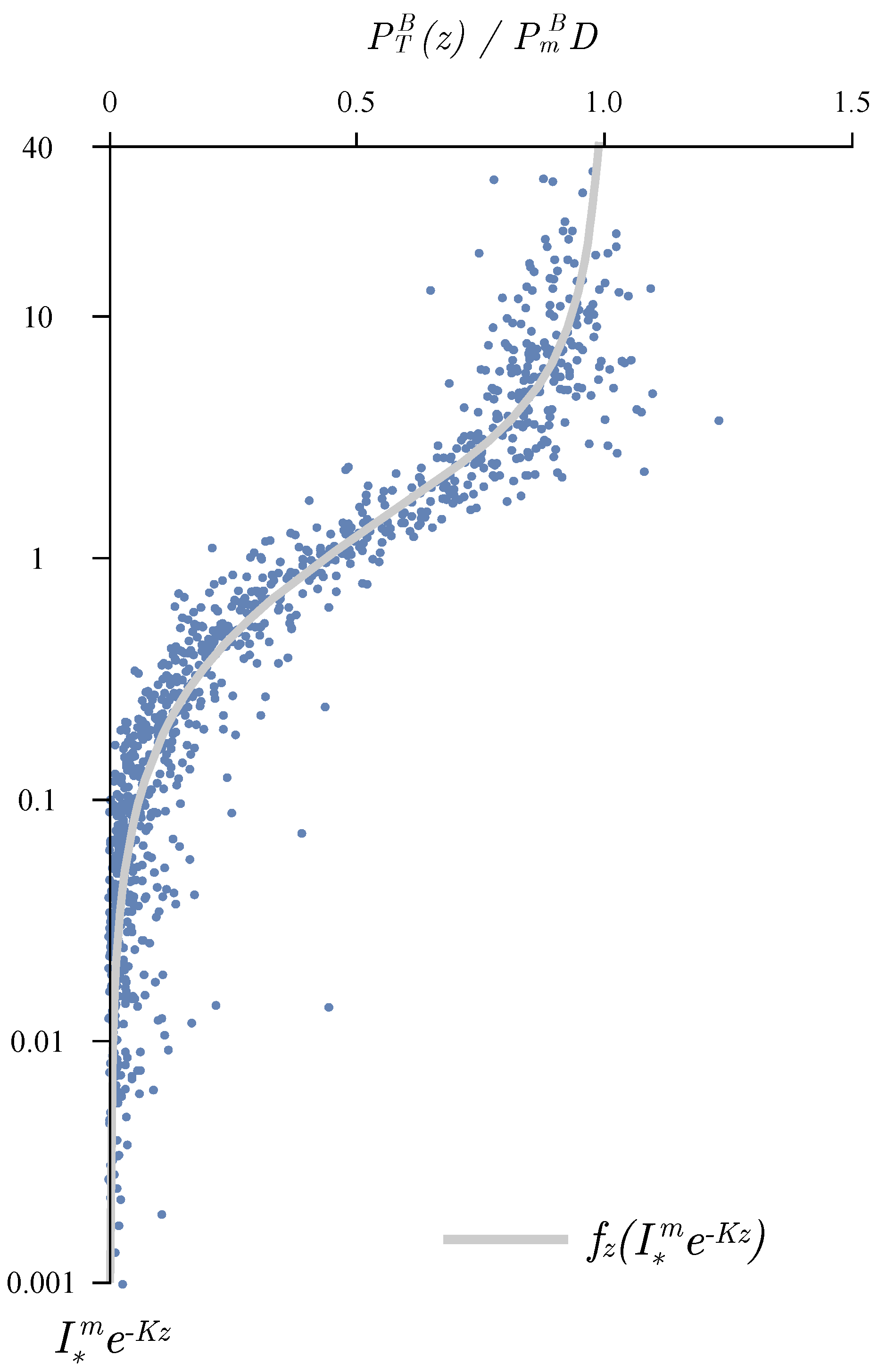
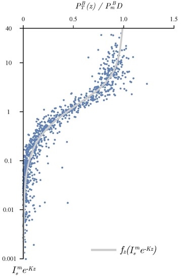
Having recovered the parameter values, we then used them in the analytical solution (8) to calculate the normalized daily production at depth. We calculated the coefficient of determination which scored a high value of 0.95, meaning 95% of variance in the data set was explained by the model. In addition, we compared all the measurements against the analytical solution, and the comparison is presented in Figure 2. The points on the figure represent the normalized production of the measured biomass divided by P m B D , plotted against I m e K z , as described in detail in Kovač et al. [20]. In total there were 1049 points. From the figure, we can see the points fall in line rather well with the analytical function (7). There are some discrepancies, but the errors are distributed evenly on either side of the model curve, implying that there is no systematic bias in the model for the daily production profile for this data set, justifying the usage of one set of photosynthesis parameters for modelling the normalized production profile at this station. The accuracy of the model was comparable, with respect to the coefficient of variation, to that found for the HOT data set—0.98 for P T B ( z ) for HOT [20] and 0.95 for P T B ( z ) for BATS (this work). These results are similar to the accuracy of photosynthesis irradiance models applied to production measured under controlled light conditions [13].

3.3. Estimation of Watercolumn Production

With the recovered parameters at hand, watercolumn production was calculated. We did so by employing the analytical solutions for watercolumn production available from the literature. Of particular interest were the canonical solution for watercolumn production [39] and the solution for watercolumn production with the biomass profile described by the shifted Gaussian function [31]. The two solutions differ with respect to the formulation of the biomass profile. The former uses B ( z ) = B , a vertically constant biomass, whereas the latter uses B ( z ) = B 0 + h / σ 2 π exp ( z z m ) 2 / 2 σ 2 . B 0 is referred to as the background biomass, h is the integral of the biomass under the Gaussian curve, z m is the depth of the biomass maximum and σ is the width of the biomass peak. The term, h / σ 2 π , is also abbreviated to H and yields the height of the biomass peak.
The canonical solution is valid for a well-mixed water column with uniform biomass, B, and is given as
P Z , T = B P m B D K f ( I m ) ,
where f ( I m ) is a known function [39], and the remaining assumptions are the same as in Section 2 of this paper. The solution for the shifted Gaussian biomass augments the canonical solution by an additional term which takes into account the excess production due to vertical variation in biomass. This solution is
P Z , T = B 0 P m B D K f ( I m ) + Δ P Z , T ,
where Δ P Z , T is the additional term, labelled the stratification term, and the exact expression for it is given in Kovač et al. [31].
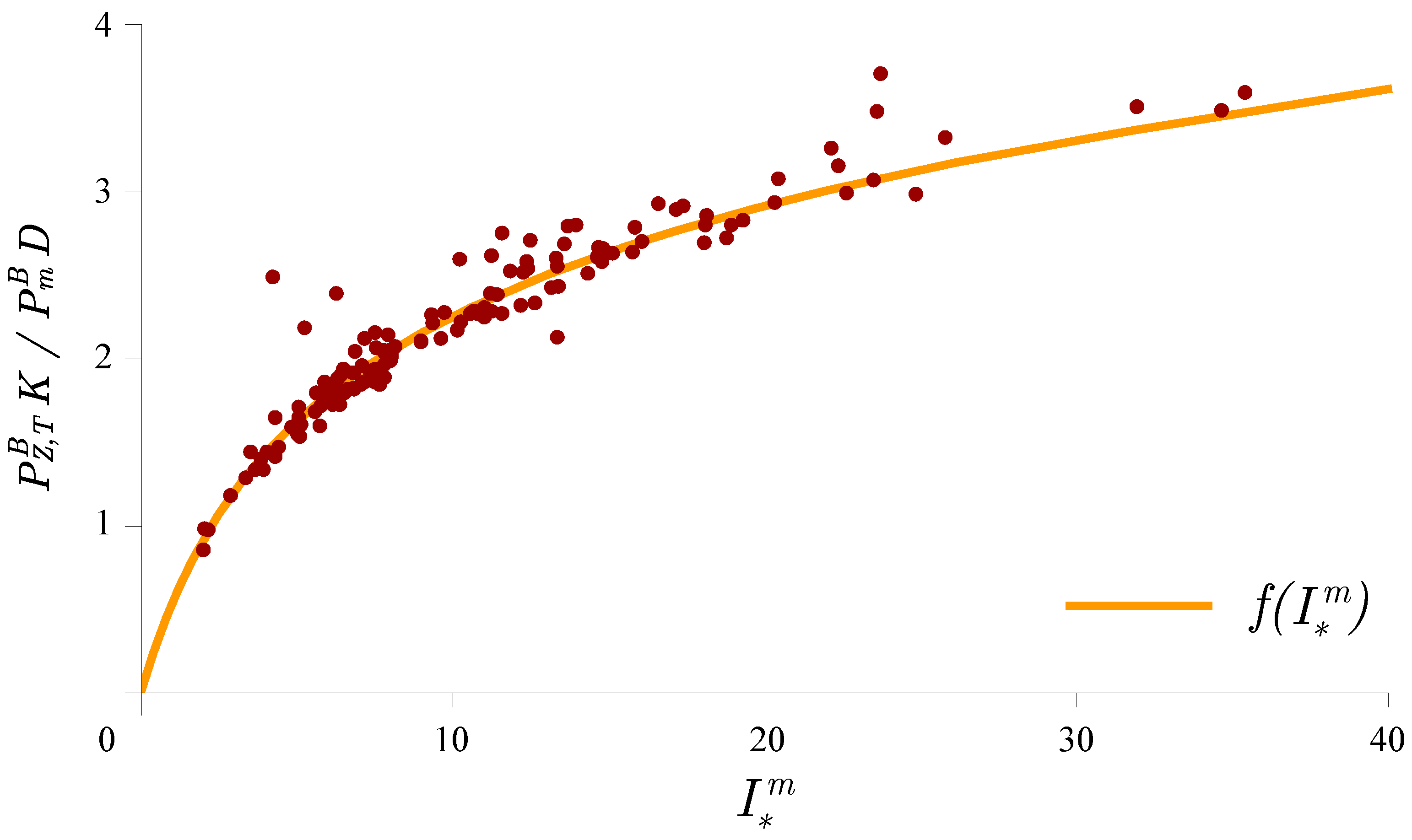
At the BATS station, the chlorophyll profile has been typically observed to vary with depth [26,41], and therefore, the canonical solution was not valid for the interval below the mixed layer. Viewed temporally, it is expected to hold for periods of the year during which the mixed layer is deep, such as the winter months at the BATS station [41]. However, it was possible to use the canonical solution to calculate the normalized daily watercolumn production, which represents the production per unit chlorophyll biomass, and hence, is independent of any variation in the chlorophyll profile. Therefore, we were able to test the canonical solution (10) in a manner similar to that in which the solution (8) was tested. The results are shown in Figure 3. Again, the points on the figure were obtained as a combination of measurements and estimated parameters, as described in detail in Kovač et al. [20]. Normalized daily watercolumn production was calculated by the trapezoidal rule from the measurements. Here, the coefficient of determination between the measured and modelled normalized daily watercolumn production was high (0.97). A similarly high coefficient of determination of 0.99 was also found at HOT for normalized watercolumn production [20]. Such high coefficients of determination at BATS and HOT demonstrate that this model structure is appropriate for computing watercolumn production.
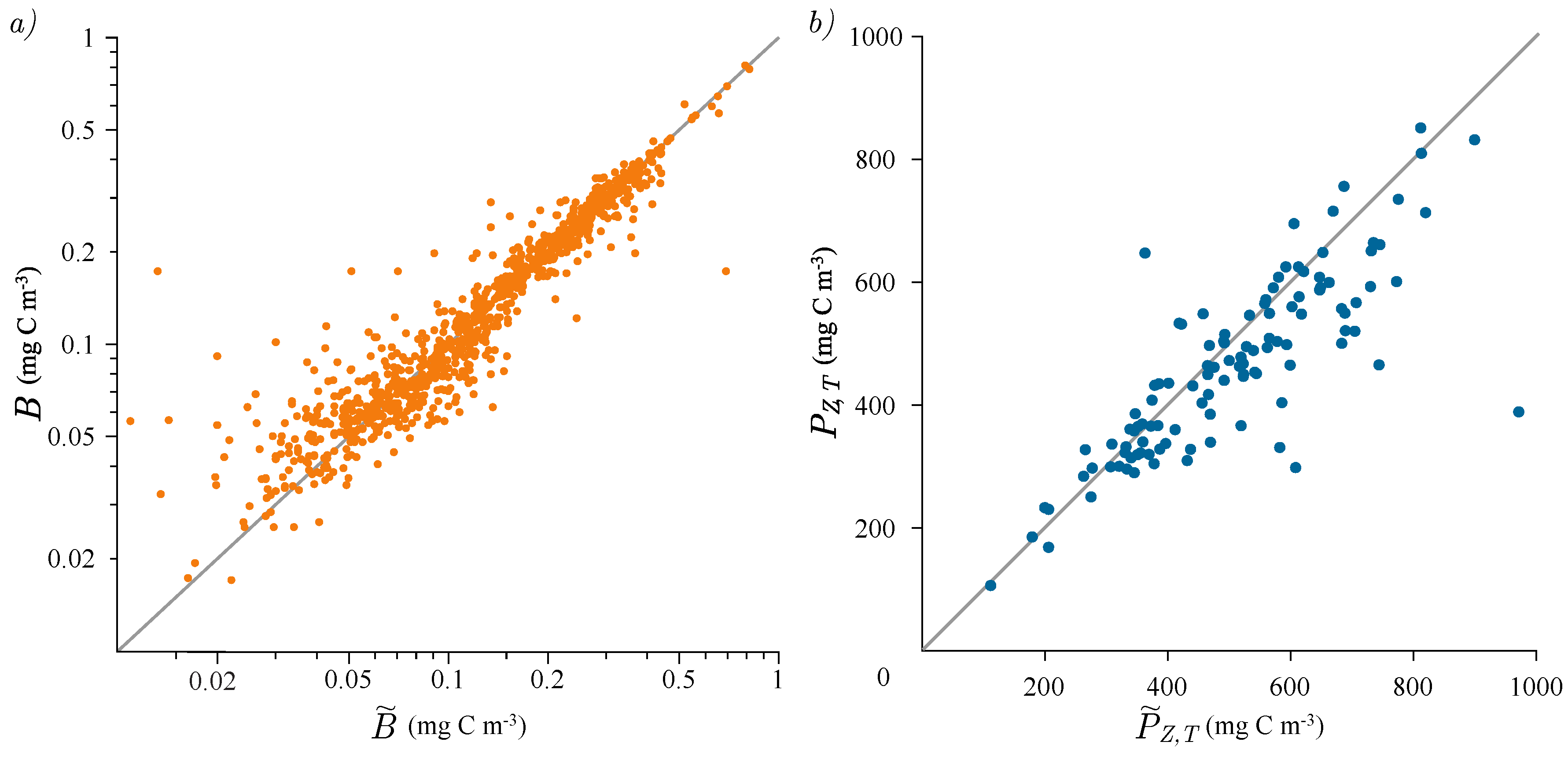
Following this, we tested the solution for watercolumn production with the biomass profile described by the shifted Gaussian (11). This solution is tailored for variable biomass profiles, such as those that include a deep chlorophyll maximum, which has been observed to be a quasi-permanent feature at the BATS station. It is known that the shifted Gaussian is a suitable function for the description of this class of biomass profiles [32,45]. Here, we fitted the shifted Gaussian function to the measured biomass profiles, and the comparison of the measured versus modelled biomass is presented in Figure 4a. Fitting was accomplished by tuning the parameters of the shifted Gaussian, namely B 0 , h, σ and z m , to best match the measured biomass profile. The conjugate gradient method was used to perform this task [46,47] and the fit of the shifted Gaussian was convergent for each chlorophyll profile. As can be seen from Figure 4a, the match between the model and the measurement was satisfactory. Quantitatively, the coefficient of determination for the entire biomass data set was 0.93. A total of 1049 chlorophyll measurements were compared with the modelled shifted Gaussian profile in the figure. This is comparable to that obtained for a similar comparison for data from HOT, where the coefficient of determination was found to be either 0.87 or 0.98, depending on whether the deepest two depths were included or excluded [31].
For the BATS station, the mean of the background biomass, B 0 , was 0.068 mg Chl m−3, with a standard deviation of 0.032 mg Chl m−3. The mean depth of the deep biomass maximum, z m , was 99 m , with a standard deviation of 21 m . The mean width of the biomass peak σ was 22 m, with a standard deviation of 12.5 m and finally, the mean height of the biomass peak, H, was 0.377 mg Chl m−3, with a standard deviation of 0.265 mg Chl m−3.
The successful description of the biomass profiles by the shifted Gaussian further justified the application of the solution (11) to calculate watercolumn production. The stratification term, Δ P Z , T , depends on h, σ , and z m , and therefore, the accuracy of the whole solution depends on these parameters. For a certain range of parameter values, this solution exhibited convergent behaviour and gave reasonable estimates of watercolumn production. In particular, when the deep chlorophyll maximum was deep and narrow, the solution converged, whereas when it was shallow and wide, it tended to diverge. As a quantitative measure of convergent behaviour, the 3 σ rule was applied, following Kovač et al. [31], where the solution was considered to be valid in situations with z m deeper than 3 σ . This is indeed the expected case for the open ocean with a deep chlorophyll maximum, and the 3 σ condition was satisfied for 116 profiles from the BATS data set. The results are displayed in Figure 4b. In the figure, we can observe some discrepancies, but an overall matching is evident.

3.4. Estimation of Growth Rates

Knowing the assimilation number enabled us to estimate the maximum growth rate of phytoplankton. Following Kirchman [48], Marañon [49] and Sathyendranath et al. [50], we defined the maximum instantaneous growth rate, μ m , attainable by a phytoplankton assemblage as
μ m = P m B χ ,
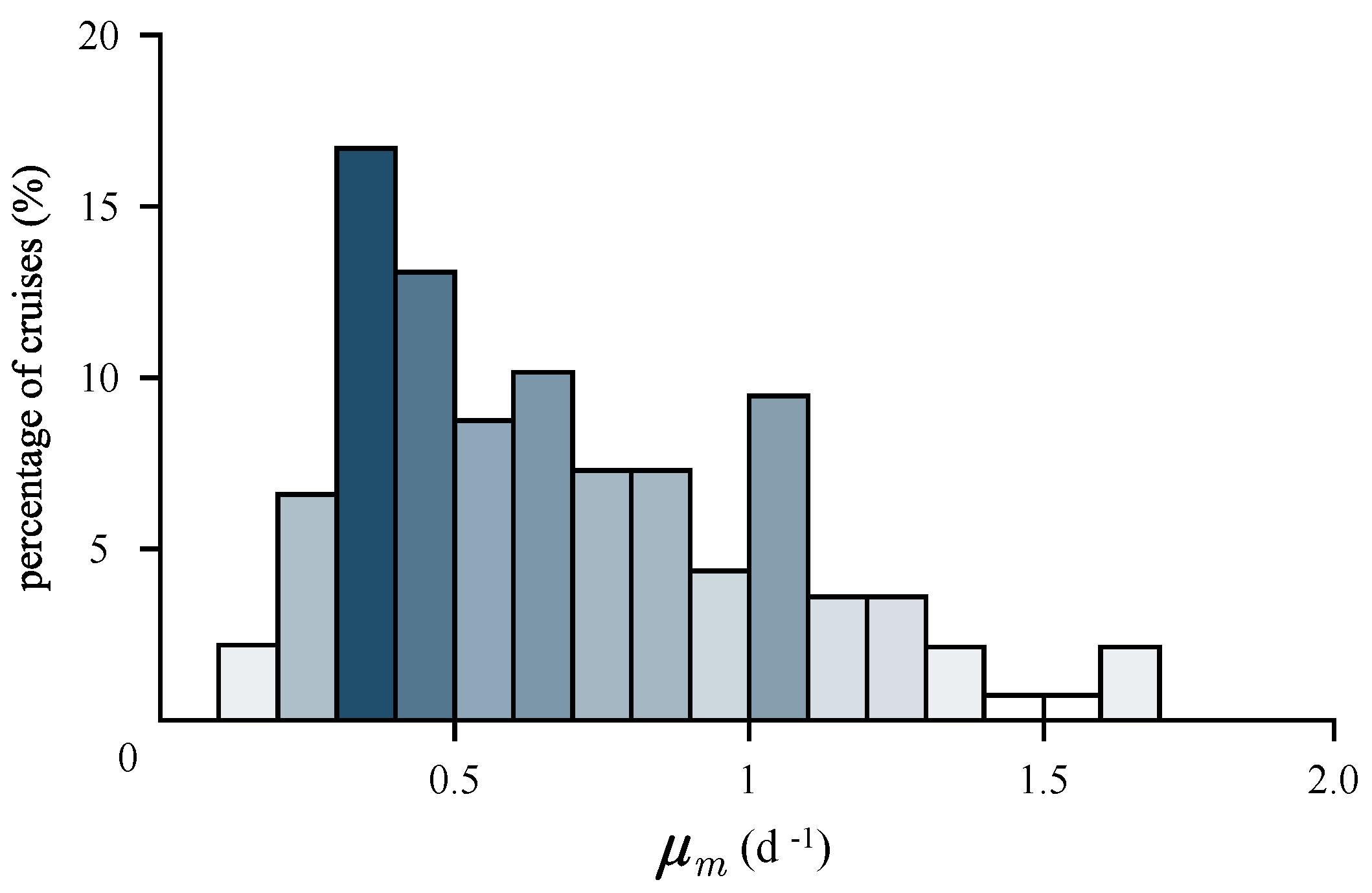
where χ is the carbon-to-chlorophyll ratio. To estimate μ m for a given production profile, we needed information on the assimilation number and the carbon-to-chlorophyll ratio. We took the carbon-to-chlorophyll ratio from Marañon [49] for the Western North Atlantic Subtropical Gyre, equal to 146 mg C (mg Chl)−1. For each cruise, we calculated μ m , and the results are given in Figure 5, expressed as per day growth rate, by multiplying the hourly rate from Equation (12) by the daylength, D. In fact, using this method, we determined the maximum daily growth rate. The distribution of the maximum daily growth rate was skewed to the right. The mean value was 0.7 d−1, the median was 0.62 d−1 and the standard deviation was 0.39 d−1. The minimum value was 0.13 d−1 and the maximum was 1.67 d−1. For 118 profiles, the maximum daily growth rate was below one per day, and for 33 profiles, it was above one per day.
The maximum instantaneous growth rates calculated here are slightly higher than those reported in Marañon [49]. However, they reported values for different regions of the Atlantic and did not calculate the μ m for our study area, due to a lack of information on P m B . Also, as stated by the author [49], his estimates were lower than those reported by other authors, such as Gasol et al. [51] and Harris [52]. His reasoning in favour of a low growth rate in the oligotrophic ocean was that phytoplankton do not have sufficiently high assimilation numbers to sustain it. As pointed out by Marañon [49], a μ m > 2.5 d−1 with χ in the range of 100–200 mg C (mg Chl)−1 requires P m B > 25 mg C (mg Chl)−1 h−1, i.e., above the theoretical maximum calculated by Falkowski [53]. Here, did not observe such high assimilation numbers (Figure 1b), but the histogram shows a right-hand tail with values well above 10 to 15 mg C (mg Chl)−1 h−1, which implies the possibility of high growth rates, at least on occasion. The bulk of our results are consistent with those of Casey et al. [54], who reported growth rates in the Sargasso Sea equal to 0.42 ± 0.17 d−1, based on nitrogen uptake rates. The reader is referred to Table 2 in Casey et al. [54] for more literature values on the growth rates in the Sargasso Sea, which are all consistent with the ones reported in this work, although obtained by different methods.
The growth rate calculated with (12) is actually an upper bound on the daily growth rate when reported as a daily rate. Expression (12) is valid for constant and saturating light conditions during the entire daylength. It therefore corresponds to the following growth equation:
d d t B ( t ) = P m B χ B ( t ) .
A more plausible approach would be to allow for the temporal dependence of production on variable light conditions and to calculate the daily growth rate accordingly. Therefore, instead of the upper bound, μ m , the daily growth rate, μ , would be used, starting with the following growth equation:
d d t B ( z , t ) = P m B χ 1 exp α B I ( z , t ) / P m B B ( z , t ) ,
with time-dependent production due to varying irradiance, I ( z , t ) = I 0 m sin ( π t / D ) exp ( K z ) , where both B and I are now recognized as functions of depth and time. With information on the initial B ( z , 0 ) and final B ( z , D ) biomass, the daily growth rate at depth z can be expressed as
μ ( z ) = 1 D ln B ( z , D ) / B ( z , 0 ) .
However, we did not have information (measurements) on the final biomass to use (15) directly, but we did have information about the daily production at depth P T ( z ) . To use this information, we expressed the final biomass as a function of the initial biomass and daily production. By integrating (14) over the daylength, D, we obtained the following expression for the final biomass [19]:
B ( z , D ) = B ( z , 0 ) exp P T B ( z ) / χ .
Upon inserting this expression into (15), we obtained the following equation for the daily growth rate:
μ ( z ) = P T B ( z ) χ D .
Going one step further and expressing P T B ( z ) as a function of depth by using solution (8) we obtained:
μ ( z ) = P m B χ f z I m e K z .
This expression shows that the daily growth rate at any given depth can be calculated from the maximum instantaneous growth rate (12) and the shape of the production profile, set by the f z I m e K z function. According to (18), the depth dependence of the growth rate is identical to the depth dependence of the normalized production profile in the case of a depth-independent carbon-to-chlorophyll ratio, χ . Whereas it is plausible to have a uniform χ in the mixed layer, it is highly unlikely that χ would remain invariant with depth in a stratified ocean. Therefore, to calculate the daily growth rate for a stratified ocean would require having χ as a function of depth χ = χ ( z ) . For a mixed layer, it may be argued that the daily growth rate should be calculated from mixed-layer production, and this has been studied extensively by Platt et al. [55], who gave explicit expressions for the mixed-layer growth rate. For an in-depth account of mixed-layer growth rate, the reader is also referred to [56,57].
Comparing (12) with (18), we recognized in the numerator of both expressions, that P m B was the maximum possible instantaneous production at depth that would occur under saturating light conditions. According to solution (8), this is never realised for the entire daylength (sunrise till sunset), because the function f z ( I m e K z ) is always less than unity and goes to unity only at the limit of I m e K z [20]. This limit is not reached in the real ocean, which is a direct consequence of the diurnal cycle of irradiance (3). As the irradiance goes from zero at dawn, to a maximum at noon, and back to zero at sunset, normalized production falls below P m B , and normalized daily production at any depth is always less than P m B D . This is why (12) gives an upper bound on the daily growth rate and (18) gives the daily growth rate, which is less than P m B / χ due to f z ( I m e K z ) being less than 1. Therefore, we expected the daily growth rate in the ocean to satisfy the condition μ < P m B / χ when expressed on a per hour basis.

3.5. Seasonal Cycle

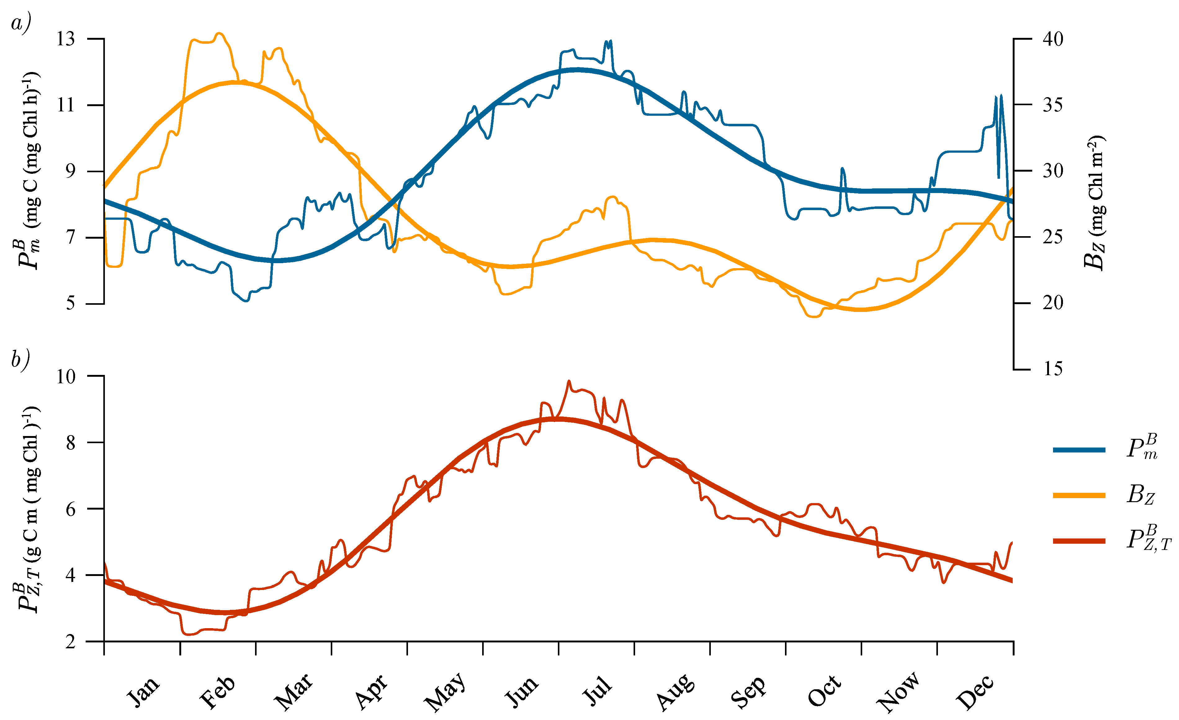
For each Julian day, we calculated the mean value of the parameters that were estimated from all cruise data measured within the interval set by 15 days before and after that Julian day, for all the years for which data were available. In such a manner, we obtained an estimate of the seasonal cycle of average monthly values of parameters. The seasonal cycle of α B was not as pronounced as the seasonal cycle of P m B . This might be because we only had 87 estimates of α B , whereas we had 151 estimates of P m B . The seasonal cycle of average monthly P m B is given in Figure 6 (thin blue curve). The minimum in P m B occurred in February, after which a steep rise led to a maximum in July. After the maximum, a less steep decline followed until the end of the year. To this seasonal cycle, we further fitted a sum of two sine functions superimposed onto a mean (Figure 6, thick blue curve). The first sine has a one year period and the second has a half-year period, given here explicitly:
P m B ( j ) = 8.8 2.0 sin 2 π j / 365 + 1.0 + 1.0 sin 4 π j / 365 4.4 ,
in units of mg C (mg Chl)−1 h−1, where j = 0 , 1 , 2 , , 365 is the Julian day. Judging by the figure, the representation of the seasonal cycle by the sum of two sine functions is well suited for the assimilation number.
We further observed that the seasonal cycle of normalized water column production was similar in shape to the seasonal cycle of the assimilation number (Figure 6, red curve). However, the similarity of the seasonal cycle of watercolumn production was not observed (Figure 7, grey curve). Upon comparing the two, a noticeable feature in the seasonal cycle of P Z , T was a rise in production starting in January and lasting during February, March and April, which has been well documented in the literature [29,30]. This was not observed in the seasonal cycle of P Z , T B , which had its minimum in February and maximum in July. To account for this rise in daily production during the period of January to April, we looked at the seasonal cycle of total chlorophyll concentration within the euphotic zone, ( B Z ) (Figure 6, orange curves), and we observed a similar elevation in B Z as in P Z , T during the same period. Therefore the increase in P Z , T can be attributed to a rise in biomass and not in P m B . This is in line with the theoretical solution (10), according to which normalized watercolumn production does not depend on B, but does depend on P m B . Following (10) we can infer that the initial slope, daylength, attenuation coefficient and noon irradiance also play roles, although perhaps not as significant as that of the assimilation number.
Further, by comparing the seasonal cycle of B Z with P m B , we observed that they were nearly in counterphase. Starting in January, biomass increased, but P m B declined and then in April, the opposite occurred, with P m B now increasing and B Z decreasing. P m B rose from March untill July, and more or less declined from August until March. On the other hand, B Z declined from February until October (with a steady period during June, July and August) and then increased from October until March. In the context of the observed annual cycle of the assimilation number (Figure 6a) we see that, although the assimilation number was low during winter, the biomass still managed to rise. These findings are consistent with Evans and Parslow [58] for the seasonal cycle in the North Atlantic. According to these authors, the deepening of the mixed layer in winter, combined with low incoming solar radiation caused a decline in the average light available for photosynthesis in the mixed layer, and consequently, a reduction in the average production per unit biomass. A reduction in normalized production was indeed observed at the BATS station (Figure 6), along with an increase in the mixed-layer depth during winter [26,41].
Another consequence of winter mixed layer deepening is the effect it has on zooplankton that graze on phytoplankton. When the mixed layer deepens and the phytoplankton are diluted, this causes a reduction of food for the zooplankton and their numbers decline. This precondition, occurring before the spring, means that when larger phytoplankton start to increase, the larger zooplankton are unable to catch up with them immediately, allowing a bloom to form. Indeed, according to Sarmiento and Gruber [59], the spring bloom at Bermuda is caused by larger phytoplankton, which are able to break free of the grazing control exerted by larger zooplankton. In addition to this, as reported from observations by Chisholm [60], picoplankton are present all year long at a more or less constant biomass in the North Atlantic near Bermuda. This implies that the grazers of smaller phytoplankton are able to catch up on a potential increase in small phytoplankton, so the smaller phytoplankton are kept in check all year long. In simpler terms, as the succession of phytoplankton proceeds over time, the phytoplankton with higher assimilation rates take over and dominate the population because their grazers are unable to catch up on their growth, which subsequently causes a rise in the assimilation number of the total population. Similar behaviour was also reported by Casey et al. [61] and Wallhead [62] and has been observed in multiple-size-class models [63].
Additionally, temperature could also have an effect on the seasonal cycle of the assimilation number. The seasonal cycle of sea surface temperature at Bermuda has been observed to be well defined, with a minimum in February and a maximum in August [30]. The timings of the minimum and maximum temperatures are well aligned with the minimum and maximum assimilation numbers. The amplitude of the seasonal cycle of sea surface temperature was observed to be about 8 C [30]. Such an amplitude could also have an effect on the assimilation number, since the enzymatic reactions underlying carbon fixation are affected by temperature [53].
Delineating these factors in more detail and decoupling the functional mechanisms would require more measurements and more complex models. Nonetheless, even the measurements we had available, although limited in spatial and temporal resolution, proved useful for the recovery of the assimilation number and the estimation of its seasonal cycle. This in itself is valuable, because prior to this study, there was no information on the seasonal cycle of the assimilation number at BATS station. With time, as more measurements become available, such estimates of the seasonal cycle will be more reliable and precise, and it will become possible to extract the seasonal cycle of the initial slope α B as well.
In an early compilation of seasonal variation in assimilation number [24], the highest assimilation number reported for the Western sub-tropical gyre was 5 mg C (mg Chl)−1 h−1, in spring. A more recent compilation [21] revised the mean value for spring slightly upwards, to 5.92, which is quite close to the value that we found for P m B in early spring (March, in Figure 6). However, instead of this being a maximum, the seasonal cycle in Figure 6 shows the value in March of ~6 mg C (mg Chl)−1 h−1 to be a minimum, with a maximum of ~12 mg C (mg Chl)−1 h−1 being reached in summer. The differences may indicate that sporadic data from ships fails to capture the full extent of seasonal variations in photosynthesis irradiance parameters, such as those revealed here. These differences have immediate implications for the computation of marine primary production based on remotely-sensed chlorophyll concentration combined with photosynthesis irradiance parameters (e.g., Sathyedranath et al. [24]).

3.6. Application to Remote Sensing

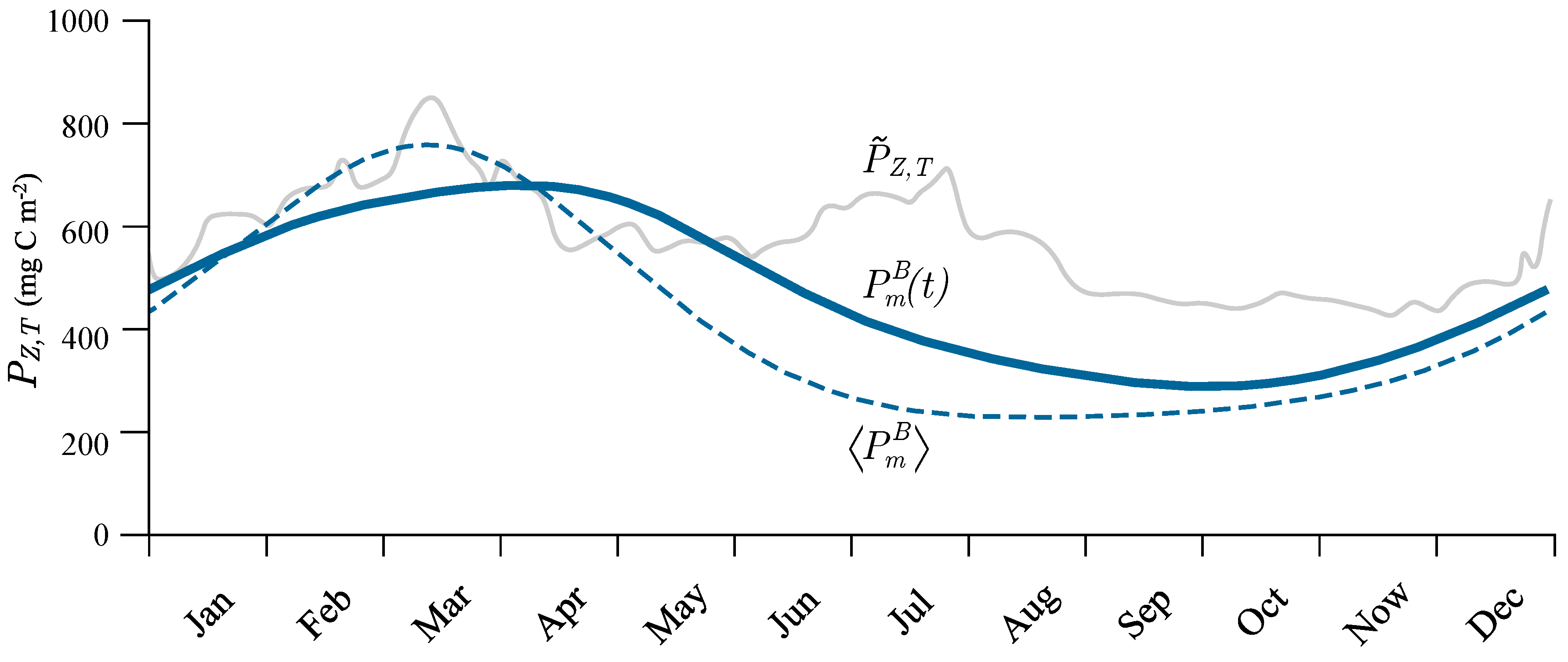
The estimated seasonal cycle of the assimilation number can be used directly to calculate primary production based on remotely-sensed chlorophyll fields, as we demonstrate here. Our goal was to model the seasonal cycle of watercolumn production with remotely-sensed chlorophyll concentration and the estimated seasonal cycle of the assimilation number. For this simple demonstration, we used the canonical solution (10) as the model for watercolumn production on each Julian day (ignoring the influence of any deep chlorophyll maximum in the interest of keeping the demonstration simple). For α B and K, we used yearly average values. We obtained the information about the chlorophyll concentration from the Ocean Colour Climate Change Initiative [64] data archives [65], which are publicly available at www.oceancolour.org. We used the monthly chlorophyll fields and estimated the seasonal cycle of remotely-sensed chlorophyll in the same manner as the seasonal cycle of the assimilation number. We calculated D and I 0 m based on the model from Kirk [34], assuming clear-sky conditions. We employed the canonical solution on each day with the seasonal cycle of the assimilation number based on the sine approximation. The results are presented in Figure 7, along with the average seasonal cycle of measured watercolumn production. In the figure, the annual cycle of primary production obtained with seasonally-varying assimiliation number is labelled P m B ( t ) , and the corresponding result based on the yearly average value of of the assimilation number is labelled P m B .
We can see there was indeed a difference between the two estimates. On average, the difference was 8%, with the maximum difference being as high as 24%. The difference was most pronounced during summer. It is also evident that estimates of watercolumn production made with P m B were generally lower compared with the ones made with P m B ( t ) . The results were in better agreement with the measured watercolumn production during winter, which was expected due to the strong mixing and resultant vertical homogeneity in the biomass, which was assumed in (10). During summer, the agreement was not as good. This may be due to three factors: firstly, remotely-sensed chlorophyll has a minimum in summer, whereas in situ surface chlorophyll does not; secondly, the contribution to watercolumn production due to the deep chlorophyll maximum could be significant; and thirdly, the seasonal variations in α B , cloud cover and the diffuse attenuation coefficient, which are ignored here, could be significant. Here, we see clear evidence that, in parts of the seasonal cycle, the stratification term, Δ P Z , T (11), is important. Nevertheless, this simple demonstration highlights the importance of assigning the correct values of photosynthesis irradiance parameters in computations of primary production using satellite data—if the computations had relied on previous archives of the parameters, the computed primary production would have been significantly lower than the observations.

4. Discussion

In this work, we built upon the previously established procedure for photosynthesis parameter recovery [16,20] by expanding it to estimate the growth rate based on the recovered photosynthesis parameters. We differentiated between the maximum instantaneous growth rate and the daily growth rate and demonstrated the connection between the two. The maximum instantaneous growth rate is defined as the ratio of the assimilation number to the carbon-to-chlorophyll ratio [50]. As such, it represents the growth of phytoplankton at its maximum capacity, as would occur under saturating light conditions. Due to the daily cycle of irradiance, which causes irradiance to drop below saturation levels, the instantaneous growth rate is, at times, below the maximum instantaneous growth rate. To account for this and to relate the daily growth rate to the maximum instantaneous growth rate, we started with a growth equation for phytoplankton, taking into account variable light conditions (14). We demonstrated that if growth effects are taken into account when calculating daily production, then a direct link between daily production and the daily growth rate emerges (17). In fact, we went a step further by providing a direct link between the maximum instantaneous growth rate and the daily growth rate (18). This was done on the premise of Equation (15), in which the daily growth rate is calculated from the logarithm of the ratio of the final to the initial biomass, divided by the time period over which it is calculated. However, some authors take a different approach.
For example, Kirchman [48] argued for not calculating the growth rate by using the expression (15), instead opting to calculate the growth rate by dividing production by the standing stock (biomass). When using (15), he employed B ( z , D ) = B ( z , 0 ) + P T ( z ) / χ , which is, in essence, the first order approximation to (16). He then went on to argue that employing (15) is correct only for low growth rates and short incubation times, in other words, the conditions for which the first order approximation holds. Here, we used a solution (16) that takes into account the positive feedback between production and biomass and is valid for any growth rate. When using (16) in (15), the daily growth rate turns out to be calculable as the ratio of production and biomass (17), which is, in essence, what Kirchman [48] advocates as the proper way of calculating the daily growth rate.
Therefore, we have demonstrated that no difference exists between growth rates calculated simply by dividing the production by the standing stock and by calculating the growth rate with (15), when the effect of growth on production is accounted for. Kirchman’s (2002) argument for dismissing (15) as the incorrect approach stemmed from using the incorrect expression for the final biomass when calculating the daily growth rate. This is, indeed, not an argument against (15); rather, it is an argument against using B ( z , D ) = B ( z , 0 ) + P T ( z ) / χ in (15). If it is acknowledged that phytoplankton increase due to production, then expression (16) for the final biomass should be used in (15).
Another detail to consider is the way in which normalized production is calculated. When using field data, normalized daily production, P T B ( z ) , is calculated by normalizing P ˜ T ( z ) to the initial biomass, thereby obtaining
P ˜ T B ( z ) = P ˜ T ( z ) / B ˜ ( z , 0 ) .
Obviously this problem does not arise in models, because normalized production is calculated with the photosynthesis irradiance function (5). To be more exact, we can use the solution for B ( z , D ) to express the daily production, P T ( z ) , in the case of the growing biomass given by (14), as in [19]:
P T ( z ) = χ B ( z , 0 ) exp 1 χ P T B ( z ) 1 .
Combining the previous two expressions gives us the measured normalized daily production on the left hand side and the model normalized daily production on the right hand side:
P ˜ T B ( z ) = χ exp P T B ( z ) / χ χ .
Therefore we see that what we measure does not, in fact, correspond to the true normalized daily production of the model if we allow for growth in biomass during the course of the period of incubation.
Consequently, if P ˜ T B ( z ) deviates significantly from the model, P T B ( z ) , a potential mismatch in the calculated daily growth rates might arise. In the case of the BATS dataset, the model-estimated production with the recovered parameters ( α B and P m B ) does not stray far from the measurements (Figure 2), and this implies the calculated growth rates will be approximately the same, whether calculated from the data or from the model-derived expression (18). However, this does come with a penalty, as the assimilation number extracted from (8) might overestimate the true assimilation number estimated from a growth model in which computed production accounted for the growing biomass. The solution for production in this case is given by (21), and we see that solution (6) is a first-order approximation to it (see details in Kovač et al. [19]). Further theoretical work is needed to expand on these considerations.
Another point worthy of discussion is the lack of sufficient data on the carbon-to-chlorophyll ratio which is required in expression (18) for each depth at which one wants to calculate μ ( z ) from P ˜ T B ( z ) , which obliged us to use a fixed value obtained from the literature to calculate the upper bound on the daily growth rate (Figure 5). An alternative approach would have been to use a photoacclimation model. In the model of Geider et al. [66], with the analytical solution presented by Jackson et al. [67], χ is an explicit function of irradiance scaled to I k :
θ = θ m I 1 exp ( I ) ,
where θ = 1 / χ , with θ m being the maximum chlorophyll-to-carbon ratio, and I = I / I k . In the case of in situ incubations, phytoplankton are maintained at a fixed depth and if we assume adaptation to average daily irradiance at that depth, then we have
I ( z ) = I 0 m exp ( K z ) D / ( 12 π I k ) .
We can now solve (23) for χ and use it directly in (18), but this only switches the problem to the lack of information on the maximum chlorophyll-to-carbon ratio θ m . However, this is a problem of practice, not of principle, and (18) could be used to calculate the daily growth rate at any depth using the retrieved I k , if θ m were known. Thanks to the parameter recovery procedure, we are now one step closer to estimating the carbon-to-chlorophyll ratio and the growth rates straight from production data measured at sea. The only information still beyond our grasp is θ m , which is required in expression (23).
A related issue is the need for to measure surface irradiance concurrently with in situ primary production measurements. These were unavailable on some cruises and consequently, we were only able to estimate the initial slope for a subset of the cruises, such that there was insufficient information to calculate a reliable parameter distribution and the seasonal cycle for both the initial slope and the photoadaptation parameter. Perhaps with time, as more complete data sets become available, the initial slope will be estimated on more cruises and the seasonal cycle will be better constrained. We might argue that it would be cheaper just to measure surface irradiance in addition to biomass and production profiles than it would be to conduct more laboratory experiments on the photosynthesis light relationship on top of measuring the production profiles to allow estimation of the initial slope. Therefore, from an economic standpoint, measuring surface irradiance routinely has definite advantages.
The surface irradiance also relates to the growth rate. When deriving (17) and (18), we assumed a sinusoidal cycle of daily irradiance. This cycle is an idealisation suitable for a clear sky, but under an overcast sky, the daily cycle changes and the total irradiance reaching the ocean surface is reduced. As a consequence, production is lower in comparison with clear sky irradiance and consequently, the daily growth rate is also lower. Paradoxically, not having an estimate of surface irradiance does not prevent us from estimating the daily growth rate directly, as we can estimate P m B and I m , and only these quantities appear in (18). Also, we can take measured normalized production directly in (17) and get the growth rate if we know χ . Again, calculating the growth rate precisely is hampered by the lack of information on the carbon-to-chlorophyll ratio.
We should emphasise here the difference between the type of parametrization of phytoplankton photosynthesis and the different types of parametrizations used in atmospheric and physical oceanographic models, which are, in essence, models based on physical laws. In these physical models, parametrizations arise in response to the inability of the models to resolve sub-grid processes [68]. Parametrizations of this sort become superfluous with increased model resolution, as the finer scale models can resolve the previously parametrized physical processes. This stands in sharp contrast to the parametrization of phytoplankton photosynthesis. Here, the parametrization of photosynthesis is itself the fundamental law and is necessary, irrespective of how fine or coarse the model grid spacing is. In essence, the parametrization of photosynthesis cannot be dispensed with on the grounds of increased resolution.
This is true not only for the model used here, but for the this whole class of primary production models. In technical terms, the model used is a canonical model, first introduced in the literature by Platt et al. [39]. Strictly speaking, a model is canonical if there is piecewise continuous transformation of variables that transforms any model into the canonical one [69]. This canonical model has the basic structure required to study the entire family of primary production models. For a more detailed description and discussion of the relationship between different models, the reader is referred to Kovač et al. [19] and Kovač et al. [31].
As a final note, we compare our results with those reported earlier. The assimilation number, P m B , reported for the Sargasso Sea by Tin et al. [9] (their Table 2) ranged from 0.88 ± 0.60 up to 7.46 ± 0.33 mg C (mg Chl)−1 h−1. The same authors [9] also reported that the initial slope, α B , ranged from 0.017 to 0.806 ± 0.46 mg C (mg Chl)−1 (W m−2)−1 h−1. These ranges coincide well with the distribution given in Figure 1. The values of P m B = 7.41 ± 2.09 mg C (mg Chl)−1 h−1 reported by Forget et al. [70] for the Sargasso Sea are also in line with the values shown in Figure 1b. However, the values reported by the same authors for α B = 0.097 ± 0.024 mg C (mg Chl)−1 (W m−2)−1 h−1 fall on the lower end of values given in Figure 1a. The numerous values for α B and P m B reported by Platt et al. [71] for the Northwest Atlantic obtained by photosynthesis light experiments all match well with the ones reported in this work. Platt et al. [71] reported that P m B went from about 1 to 12 mg C (mg Chl)−1 h−1 and α B from roughly 0.01 to 0.2 mg C (mg Chl)−1 (W m−2)−1 h−1 (the reader is referred to Figure 3a in Platt et al. [71]). We conclude that the values recovered here from in situ production measurements are in a reasonable range for the open ocean and are consistent with previous, direct estimates based on photosynthesis irradiance measurements at sea.
These results have direct implications for the remote sensing of primary production from satellite data. In comparison, Sathyedranath et al. [24] assigned α B as 0.06 to 0.11 mg C (mg Chl)−1 (W m−2)−1 h−1 and P m B as 1.7 to 5.0 mg C (mg Chl)−1 h−1 for this region of the Atlantic. According to the results presented here (Figure 1), these P m B values fall in the lower end of the parameter distributions. Furthermore, rather than applying fixed values for the assimilation number for each season, our results (Figure 7) allowed a smoothly-varying function to be applied to account for seasonal variation in the parameter when computing primary production using satellite data. These considerations further emphasise the importance of being able to evaluate the seasonal cycle in α B as well.

5. Conclusions

The presented work dealt with the estimation of photosynthesis parameters from primary production data collected at BATS over the past 30 years. This region of the Atlantic has been well studied experimentally, with a rich archive of in situ primary production measurements [41], but data on photosynthesis parameters are scarce. This is a consequence of the strategies adopted by research institutions [72], which have opted either to measure primary production in situ, or under controlled light conditions, seldom performing both experiments simultaneously. As a result, some time series stations, such as BATS, have a rich data set of in situ primary production measurements, but only a limited data set of photosynthesis parameters.
The parameter recovery procedure applied here established an archive of photosynthesis parameters for BATS (Figure 1). The recovered parameters were firstly used to model primary production and to test the adequacy of this model in accurately predicting primary production. The overall accuracy in terms of the coefficient of determination was 0.95 for production at depth and 0.97 for watercolumn production. Also, the chlorophyll-depth relation was described with the shifted Gaussian function, which accounted for 0.93 of variance in the measured chlorophyll profiles. Together, such high coefficients of determination demonstrate that this model can accurately calculate primary production at BATS.
The recovered values of the assimilation number were further used to estimate the maximum potential growth rate (Figure 5), which was previously unknown for this region due to a lack of information on the assimilation number [49]. A mathematical relationship between the maximum instantaneous growth rate and the daily growth rate was also derived (18). A lack of sufficient data on the carbon-to-chlorophyll ratio prevented a more in-depth calculation of the daily growth rates based on the measured production at each depth. Linking the carbon-to-chlorophyll ratio to the growth rate and how it relates to primary production measurements is a potential course for future research.
The seasonal cycle of the assimilation number was estimated, and it was observed to be nearly in counterphase with the chlorophyll seasonal cycle. The highest values of the assimilation number were observed during June, July and August, while the lowest were observed during January, February and March. It was also demonstrated that the seasonal cycle of the assimilation number can be well described by a sum of two sine functions. The utility of this description is that it can easily be used in remote sensing applications to model primary production at this station, as was demonstrated in Figure 7.

Author Contributions

All authors conceived and designed the study. M.L. assisted in acquiring the data. Ž.K. implemented the model and wrote the draft. Ž.K., T.P., S.S. and M.L. wrote the final manuscript. All authors have read and approved the submitted manuscript.

Acknowledgments

This work was supported, in part, by Croatian Science Foundation under the project MARIPLAN (IP-2014-09-3606). This work is a contribution to the European Space Agency Projects “STSE Marine Primary Production: Model Parameters from Space” and “SEOM Photosynthetically Active Radiation for Primary Production”. Additional support from the National Centre for Earth Observation of the Natural Environment Research Council (UK) is also acknowledged. T.P. acknowledges the support provided by a Jawaharlal Nehru Science Fellowship (Government of India). We also acknowledge the support of Simons Foundation through the CBIOMES Project. We thank the National Science Foundation Chemical and Biological Oceanography Programs for continued support of the BATS program through the following awards: OCE 88–01089, OCE 93–01950, OCE 9617795, OCE 0326885, OCE 0752366, and OCE-0801991. We acknowledge the BATS and the BBOP for the publicly available database. We thank their scientists and staff.

Conflicts of Interest

The authors declare no conflict of interest.

References

  1. Steemann Nielsen, E. The use of radioactive carbon (C14) for measuring organic production in the sea. ICES J. Mar. Sci. 1952, 18, 117–140. [Google Scholar] [CrossRef]
  2. Platt, T.; Denman, K.L.; Jassby, A.D. Modelling the productivity of phytoplankton. In The Sea: Ideas and Observations on Progress in the Study of the Seas; Wiley: New York, NY, USA, 1977; pp. 807–856. [Google Scholar]
  3. Platt, T.; Gallegos, C.L. Modelling primary production. In Environmental Science Research; Plenum Publishing Corporation: New York, NY, USA, 1980; pp. 339–362. [Google Scholar]
  4. Longhurst, A.; Sathyendranath, S.; Platt, T. An estimate of global primary production in the ocean from satellite radiometer data. J. Plankton Res. 1995, 17, 1245–1271. [Google Scholar] [CrossRef]
  5. Antoine, D.; Andre, J.M.; Morel, A. Oceanic primary production 2. Estimation at global scale from satellite (coastal zone color scanner) chlorophyll. Glob. Biogeochem. Cycles 1996, 10, 57–69. [Google Scholar] [CrossRef]
  6. Westberry, T.; Behrenfeld, M.J.; Siegel, D.A.; Boss, E. Carbon-based primary productivity modeling with vertically resolved photoacclimation. Glob. Biogeochem. Cycles 2008, 22, GB2024. [Google Scholar] [CrossRef]
  7. Buitenhuis, E.T.; Hashioka, T.; Quéré, L. Combined constraints on global ocean primary production using observations and models. Glob. Biogeochem. Cycles 2013, 27, 847–858. [Google Scholar] [CrossRef] [Green Version]
  8. Sathyendranath, S.; Platt, T. Remote sensing of water-column primary production. ICES Mar. Sci. Symp. 1993, 197, 236–243. [Google Scholar]
  9. Tin, H.; Lomas, M.; Ishizaka, J. Satellite-derived estimates of primary production during the Sargasso Sea winter/spring bloom: Integration of in-situ time-series data and ocean color remote sensing observations. Reg. Stud. Mar. Sci. 2016, 3, 131–143. [Google Scholar] [CrossRef]
  10. Behrenfeld, M.J.; Boss, E.; Siegel, D.A.; Shea, D.M. Carbon-based ocean productivity and phytoplankton physiology from space. Glob. Biogeochem. Cycles 2005, 19, GB1006. [Google Scholar] [CrossRef]
  11. Platt, T.; Jassby, A. The relationship between photosynthesis and light for natural assemblages of coastal marine phytoplankton. J. Phycol. 1976, 12, 421–430. [Google Scholar] [CrossRef]
  12. Jassby, A.D.; Platt, T. Mathematical formulation of the relationship between photosynthesis and light for phytoplankton. Limnol. Oceanogr. 1976, 21, 540–547. [Google Scholar] [CrossRef] [Green Version]
  13. Jones, C.T.; Craig, S.E.; Barnett, A.B.; MacIntyre, H.L.; Cullen, J.J. Curvature in models of the photosynthesis-irradiance response. J. Phycol. 2014, 50, 341–355. [Google Scholar] [CrossRef] [PubMed] [Green Version]
  14. Platt, T.; Sathyendranath, S. Fundamental issues in measurement of primary production. ICES Mar. Sci. Symp. 1993, 197, 3–8. [Google Scholar]
  15. Sakshaug, E.; Bricaud, A.; Dandonneau, Y.; Falkowski, P.; Kiefer, D.A.; Legendre, L.; Morel, A.; Parslow, J.; Takahashi, M. Parameters of photosynthesis: Definitions, theory and interpretation of results. J. Plankton Res. 1997, 19, 1637–1670. [Google Scholar] [CrossRef]
  16. Kovač, Ž.; Platt, T.; Sathyendranath, S.; Morović, M.; Jackson, T. Recovery of photosynthesis parameters from in situ profiles of phytoplankton production. ICES J. Mar. Sci. 2016, 73, 275–285. [Google Scholar] [CrossRef]
  17. Peterson, B.J. Aquatic primary production and the 14C-CO2 method: A history of the productivity problem. Annu. Rev. Ecol. Evol. Syst. 1980, 11, 359–385. [Google Scholar] [CrossRef]
  18. Barber, R.T.; Hilting, A.K. History of the study of plankton productivity. In Phytoplankton Productivity–Carbon Assimilation in Marine and Freshwater Ecosystems; Blackwell Science: Hoboken, NJ, USA, 2002; pp. 16–43. [Google Scholar] [CrossRef]
  19. Kovač, Ž.; Platt, T.; Sathyendranath, S.; Antunović, S. Models for estimating photosynthesis parameters from in situ production profiles. Prog. Oceanogr. 2017, 159, 255–266. [Google Scholar] [CrossRef]
  20. Kovač, Ž.; Platt, T.; Sathyendranath, S.; Morović, M. Analytical solution for the vertical profile of daily production in the ocean. J. Geophys. Res. Oceans 2016, 121. [Google Scholar] [CrossRef]
  21. Bouman, H.; Platt, T.; Doblin, M.; Figueiras, F.G.; Gudmundsson, K.; Gudfinnsson, H.; Huang, B.; Hickman, A.; Hiscock, M.; Jackson, T.; et al. Photosynthesis-irradiance parameters of marine phytoplankton: Synthesis of a global data set. Earth Syst. Sci. Data 2017, 10, 251–266. [Google Scholar] [CrossRef]
  22. Platt, T.; Sathyendranath, S. Biological production models as elements of coupled, atmosphere-ocean models for climate research. J. Geophys. Res. 1991, 96, 2585–2592. [Google Scholar] [CrossRef]
  23. Franks, P.J.S. NPZ Models of plankton dynamics: Their construction, coupling to physics, and application. J. Oceanogr. 2002, 58, 379–387. [Google Scholar] [CrossRef]
  24. Sathyedranath, S.; Longhurst, A.; Caverhill, C.M.; Platt, T. Regionally and seasonally differentiated primary production in the North Atlantic. Deep Sea Res. Part I 1995, 42, 1773–1802. [Google Scholar] [CrossRef]
  25. Karl, D.M.; Lukas, R. The Hawaii Ocean Time-series (HOT) program: Background, rationale and field implementation. Deep Sea Res. Part II 1996, 43, 129–156. [Google Scholar] [CrossRef]
  26. Steinberg, D.K.; Carlson, C.A.; Bates, N.R.; Johnson, R.J.; Michaels, A.F.; Knap, A.H. Overview of the US JGOFS Bermuda Atlantic Time-series Study (BATS): a decade-scale look at ocean biology and biogeochemistry. Deep Sea Res. Part II 2001, 48, 1405–1447. [Google Scholar] [CrossRef]
  27. Muller-Karger, F.; Varela, R.; Thunell, R.; Scranton, M.; Bohrer, R.; Taylor, G.; Capelo, J.; Astor, Y.; Tappa, E.; Ho, T.Y.; et al. Annual cycle of primary production in the Cariaco Basin: Response to upwelling and implications for vertical export. J. Geophys. Res. 2001, 106, 4527–4542. [Google Scholar] [CrossRef] [Green Version]
  28. Pennington, J.T.; Chavez, F.P. Seasonal fuctuations of temperature, salinity, nitrate, chlorophyll and primary production at station H3/M1 over 1989-1996 in Monterey Bay, California. Deep Sea Res. Part II 2000, 47, 947–973. [Google Scholar] [CrossRef]
  29. Chavez, F.P.; Messié, M.; Pennington, J.T. Marine Primary Production in Relation to Climate Variability and Change. Ann. Rev. Mar. Sci. 2011, 3, 227–260. [Google Scholar] [CrossRef] [PubMed]
  30. Church, M.J.; Lomas, M.W.; Muller-Karger, F. Sea change: Charting the course for biogeochemical ocean time-series research in a new millennium. Deep Sea Res. Part II 2013, 93, 2–14. [Google Scholar] [CrossRef]
  31. Kovač, Ž.; Platt, T.; Antunović, S.; Sathyendranath, S.; Morović, M.; Gallegos, C. Extended Formulations and Analytic Solutions for Watercolumn Production Integrals. Front. Mar. Sci. 2017, 4, 163. [Google Scholar] [CrossRef]
  32. Longhurst, A.R. Ecological Geography of the Sea, 2nd ed.; Academic Press: Cambridge, MA, USA, 1998. [Google Scholar]
  33. Mignot, A.; Claustre, H.; Uitz, J.; Poteau, A.; D’Ortenzio, F.; Xing, X. Understanding the seasonal dynamics of phytoplankton biomass and the deep chlorophyll maximum in oligotrophic environments: A Bio-Argo float investigation. Glob. Biogeochem. Cycles 2014, 28, 856–876. [Google Scholar] [CrossRef] [Green Version]
  34. Kirk, J.T.O. Light and Photosynthesis in Quatic Ecosystems, 3rd ed.; Cambridge University Press: Cambridge, UK, 2011. [Google Scholar] [CrossRef]
  35. Sathyendranath, S.; Platt, T. The spectral irradiance field at the surface and in the interior of the ocean: A model for applications in oceanography and remote sensing. J. Geophys. Res. 1988, 93, 9270–9280. [Google Scholar] [CrossRef]
  36. Platt, T.; Sathyendranath, S.; White, G.N.; Ravindran, P. Attenuation of visible light by phytoplankton in a vertically structured ocean: solutions and applications. J. Plankton Res. 1994, 16, 1461–1487. [Google Scholar] [CrossRef]
  37. Platt, T.; Sathyendranath, S. Estimators of Primary Production for Interpretation of Remotely Sensed Data on Ocean Color. J. Geophys. Res. 1993, 98, 14561–14576. [Google Scholar] [CrossRef]
  38. Frenette, J.; Demers, S.; Legendre, L. Lack of agreement among models for estimating the photosynthetic parameters. Limnol. Oceanogr. 1993, 38, 679–687. [Google Scholar] [CrossRef]
  39. Platt, T.; Sathyendranath, S.; Ravindran, P. Primary Production by Phytoplankton: Analytic Solutions for Daily Rates per Unit Area of Water Surface. Proc. R. Soc. B 1990, 241, 101–111. [Google Scholar] [CrossRef]
  40. Platt, T.; Gallegos, C.L.; Harrison, W.G. Photoinhibition of photosynthesis in natural assemblages of marine phytoplahnkton. J. Mar. Res. 1980, 38, 687–701. [Google Scholar]
  41. Michaels, A.F.; Knap, A.H. Overview of the U.S. JGOFS Bermuda Atlantic Time-series Study and the Hydrostation S Program. Deep Sea Res. Part II Top. Stud. Oceanogr. 1996, 43, 157–198. [Google Scholar] [CrossRef]
  42. Morel, A.; Smith, R.C. Relation between total quanta and total energy for aquatic photosynthesis. Limnol. Oceanogr. 1974, 19, 591–600. [Google Scholar] [CrossRef]
  43. Allen, J.G.; Nelson, N.B.; Siegel, D.A. Seasonal to multi-decadal trends in apparent optical properties in the Sargasso Sea. Deep Sea Res. Part I Oceanogr. Res. Pap. 2017, 119, 58–67. [Google Scholar] [CrossRef]
  44. Lomas, M.W.; Bates, N.R.; Johnson, R.J.; Knap, A.H.; Steinberg, D.K.; Carlson, C.A. Two decades and counting: 24-years of sustained open ocean biogeochemical measurements. Deep Sea Res. II 2013, 93, 16–32. [Google Scholar] [CrossRef]
  45. Platt, T.; Caverhill, C.; Sathyendranath, S. Basin-scale estimates of oceanic primary production by remote sensing: The North Atlantic. J. Geophys. Res. 1991, 96, 15147–15159. [Google Scholar] [CrossRef]
  46. Baldick, R. Applied Optimization: Formulation and Algorithms for Engineering Systems, 1st ed.; Cambridge University Press: Cambridge, UK, 2006. [Google Scholar]
  47. Knyazev, A.V.; Lashuk, I. Steepest Descent and Conjugate Gradient Methods with Variable Preconditioning. SIAM J. Matrix Anal. Appl. 2008, 29, 1267–1281. [Google Scholar] [CrossRef]
  48. Kirchman, D.L. Calculating microbial growth rates from data on production and standing stocks. Mar. Ecol. Prog. Ser. 2002, 233, 303–306. [Google Scholar] [CrossRef] [Green Version]
  49. Marañon, E. Phytoplankton growth rates in the Atlantic subtropical gyres. Limnol. Oceanogr. 2005, 50, 299–310. [Google Scholar] [CrossRef] [Green Version]
  50. Sathyendranath, S.; Stuart, V.; Nair, A.; Oka, K.; Nakane, T.; Bouman, H.; Forget, M.; Maass, H.; Platt, T. Carbon-to-chlorophyll ratio and growth rate of phytoplankton in the sea. Mar. Ecol. Prog. Ser. 2009, 383, 73–84. [Google Scholar] [CrossRef] [Green Version]
  51. Gasol, J.M.; del Giorgio, P.A.; Duarte, C.M. Biomass distribution in marine planktonic communities. Limnol. Oceanogr. 1997, 42, 1353–1363. [Google Scholar] [CrossRef] [Green Version]
  52. Harris, G.P. Phytoplankton productivity and growth measurements: past, present and future. J. Plankton Res. 1984, 6, 219–237. [Google Scholar] [CrossRef]
  53. Falkowski, P.G. Light-shade adaptation and assimilation numbers. J. Plankton Res. 1981, 3, 203–216. [Google Scholar] [CrossRef]
  54. Casey, J.R.; Lomas, M.W.; Mandecki, J.; Walker, D.E. Prochlorococcus contributes to new production in the Sargasso Sea deep chlorophyll maximum. Geophys. Res. Lett. 2007, 34, L10604. [Google Scholar] [CrossRef]
  55. Platt, T.; Bird, D.F.; Sathyendranath, S. Critical depth and marine primary production. Proc. R. Soc. B 1991, 246, 205–217. [Google Scholar] [CrossRef]
  56. Sathyendranath, S.; Platt, T. New production and mixed-layer physics. Proc. Indian Acad. Sci. Earth Planet. 1994, 103, 177–188. [Google Scholar] [CrossRef]
  57. Platt, T.; Sathyendranath, S. Latitude as a factor in the calculation of primary production. In Ecology of Fjords and Coastal Waters: Proceedings of the Mare Nor Symposium on the Ecology of Fjords and Coastal; Elsevier: New York, NY, USA, 1995; pp. 3–13. [Google Scholar]
  58. Evans, G.T.; Parslow, J.S. Model of Annual Plankton Cycles. Biol. Oceanogr. 1985, 3, 327–347. [Google Scholar] [CrossRef]
  59. Sarmiento, J.L.; Gruber, N. Ocean Biogeochem. Cycles, 1st ed.; Princeton University Press: Princeton, NJ, USA, 2006. [Google Scholar]
  60. Chisholm, S.W. Phytoplankton Size. In Primary Productivity and Biogeochemical Cycles in the Sea; Plenum Press: New York, NY, USA, 1992; pp. 213–237. [Google Scholar]
  61. Casey, J.R.; Aucan, J.P.; Goldberg, S.R.; Lomas, M.W. Changes in partitioning of carbon amongst photosynthetic pico- and nano-plankton groups in the Sargasso Sea in response to changes in the North Atlantic Oscillation. Deep Sea Res. Part II Top. Stud. Oceanogr. 2013, 93, 58–70. [Google Scholar] [CrossRef]
  62. Wallhead, P.J. Long-term variability of phytoplankton carbon biomass in the Sargasso Sea. Glob. Biogeochem. Cycles 2014, 28, 1–17. [Google Scholar] [CrossRef]
  63. Armstrong, R.A. Grazing limitation and nutrient limitation in marine ecosystems: Steady state solutions of an ecosystem model with multiple food chains. Limnol. Oceanogr. 1994, 39, 597–608. [Google Scholar] [CrossRef]
  64. Sathyendranath, S.; Brewin, R.J.W.; Jackson, T.; Mélin, F.; Platt, T. Ocean-colour products for climate-change studies: What are their ideal characteristics? Remote Sens. Environ. 2017, 203, 125–138. [Google Scholar] [CrossRef]
  65. Sathyendranath, S.; Groom, S.; Grant, M.; Brewin, R.; Thompson, A.; Chuprin, A.; Horseman, A.; Jackson, T.; Martinez Vicente, V.; Platt, T.; et al. ESA Ocean Colour Climate Change Initiative: Version 3.1; Centre for Environmental Data Analysis: Didcot, UK, 1 June 2018. [Google Scholar]
  66. Geider, R.J.; Macintyre, H.L.; Kana, T.M. Dynamic model of phytoplankton growth and acclimation: responses of the balancedgrowth rate and chlorophyll a:carbon ratio to light, nutrient-limitation and termperature. Mar. Ecol. Prog. Ser. 1997, 148, 187–200. [Google Scholar] [CrossRef]
  67. Jackson, T.; Sathyendranath, S.; Platt, T. An Exact Solution For Modeling Photoacclimation of the Carbon-to-Chlorophyll Ratio in Phytoplankton. Front. Mar. Sci. 2017, 4, 283. [Google Scholar] [CrossRef]
  68. Cushman-Roisin, B.; Beckers, J.M. Introduction to Geophysical Fluid Dynamics: Physical and Numerical Aspects, 2nd ed.; Academic Press: Cambridge, MA, USA, 2011. [Google Scholar]
  69. Izhikevich, E.M. Dynamical Systems in Neuroscience: The Geometry of Excitability and Bursting, 1st ed.; MIT Press: Cambridge, MA, USA, 2007. [Google Scholar] [CrossRef]
  70. Forget, M.H.; Sathyendranath, S.; Platt, T.; Pommier, J.; Vis, C.; Kyewalyanga, M.S.; Hudon, C. Extraction of photosynthesis-irradiance parameters from phytoplankton production data: Demonstration in various aquatic systems. J. Plankton Res. 2007, 29, 249–262. [Google Scholar] [CrossRef]
  71. Platt, T.; Sathyendranath, S.; Ulloa, O.; Harrison, W.G.; Hoepffner, N.; Goes, J. Nutrient control of phytoplankton photosynthesis in the Western North Atlantic. Nature 1992, 356, 229–231. [Google Scholar] [CrossRef]
  72. Platt, T.; Sathyendranath, S.; White, G.N.; Jackson, T.; Saux Picart, S.; Bouman, H. Primary Production: Sensitivity to Surface Irradiance and Implications for Archiving Data. Front. Mar. Sci. 2017, 4, 387. [Google Scholar] [CrossRef]
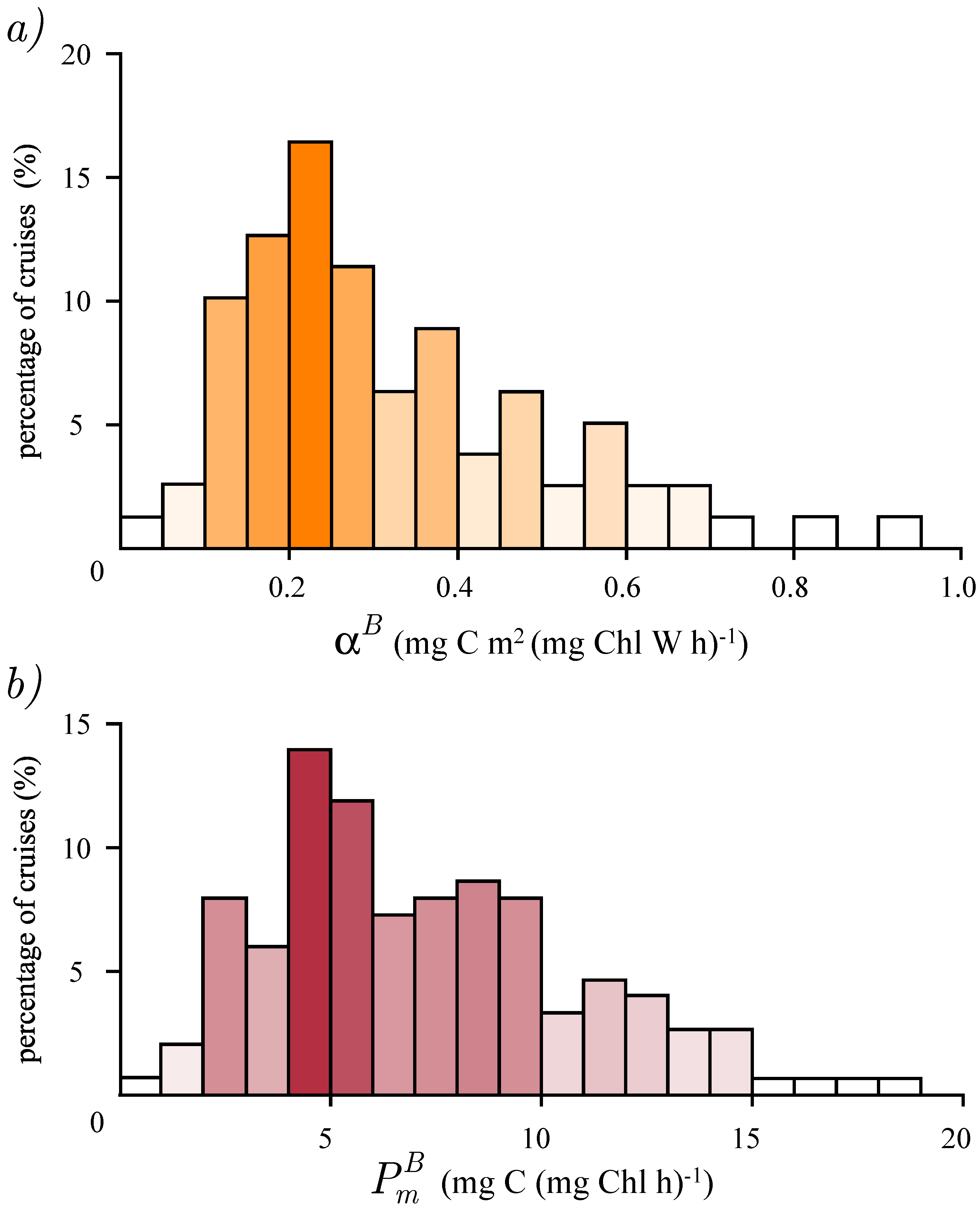
Figure 1. Histograms of estimated parameter values: (a) distribution of the initial slope, α B , obtained from 87 cruises and (b) distribution of the assimilation number, P m B , obtained from 138 cruises. The abscissa corresponds to the parameter values and the ordinate gives the percentage of cruises that fell into a certain interval of parameter values.
Remotesensing 10 00915 g001
Figure 2. Comparison of the model versus measured production at depth obtained by combining the measured data with the estimated parameter values. The abscissa corresponds to the ratio of daily production at depth P T B ( z ) to the maximum possible production, P m B D . The ordinate gives the dimensionless irradiance, I m e K z . The continuous curve is recognized as the f z ( I m e K z ) function. The coordinates of each point are ( P ˜ T B ( z n ) / P m B D , α B I ˜ 0 m e K ˜ z n / P m B ) , where α B and P m B are the estimated parameters for each profile. The r 2 value between the measured normalized production and the modeled normalized production is 0.95. In total, there are 1049 points.
Remotesensing 10 00915 g002
Figure 3. Comparison of the model and measured normalized daily watercolumn production obtained by combining the measured data with the estimated parameter values. The abscissa is the dimensionless irradiance, I m , and the ordinate is the ratio of normalized watercolumn production to P m B D / K . The continuous curve is the f ( I m ) function (10). The coordinates of each point are ( P ˜ Z , T B K ˜ / P m B D , α B I ˜ 0 m / P m B ) , where α B and P m B are the estimated parameters for each profile. The r 2 between the measured normalized watercolumn production and the modeled normalized watercolumn production is 0.97.
Remotesensing 10 00915 g003
Figure 4. (a) Scatter plot of measured B ˜ and modelled biomass B with the shifted Gaussian function. There are, in total, 1049 points. (b) Scatter plot of measured P ˜ Z , T and modeled P Z , T watercolumn production with the analytical solution for the shifted Gaussian biomass. There are, in total, 138 points. The grey line on both plots represents the 1:1 model versus the measurement ratio.
Remotesensing 10 00915 g004
Figure 5. Histogram of the estimated maximum daily growth rate, μ m , obtained from 138 cruises based on Equation (12) and here multiplied by the daylength, D, to convert hourly into daily rates. The value of the carbon-to-chlorophyll ratio χ is 146 mg C (mg Chl)−1, taken from Maranon (2005).
Remotesensing 10 00915 g005
Figure 6. Estimated seasonal cycles for the BATS station. The thin curves represent the monthly averages on each Julian day, which were calculated from the daily values, 15 days prior and 15 days post a given Julian day. The thick curves are the fits of a sum of two sine functions (superimposed onto an annual mean) to the monthly averages. (a) Seasonal cycle of P m B (blue) and B Z (orange). (b) Seasonal cycle of P Z , T B (red).
Remotesensing 10 00915 g006
Figure 7. Comparison of the measured (grey curve) versus the modelled seasonal cycle of watercolumn production based on remotely sensed-chlorophyll with the time-dependent assimilation number, P m B ( t ) (blue curve), and the average assimilation number, P m B (dashed blue curve).
Remotesensing 10 00915 g007