What Is the Spatial Resolution of grace Satellite Products for Hydrology?


Abstract
1. Introduction
2. Spherical Harmonic Coefficients and Their Corresponding Spatial Resolution
2.1. Sampling and Half-Wavelength of the Field
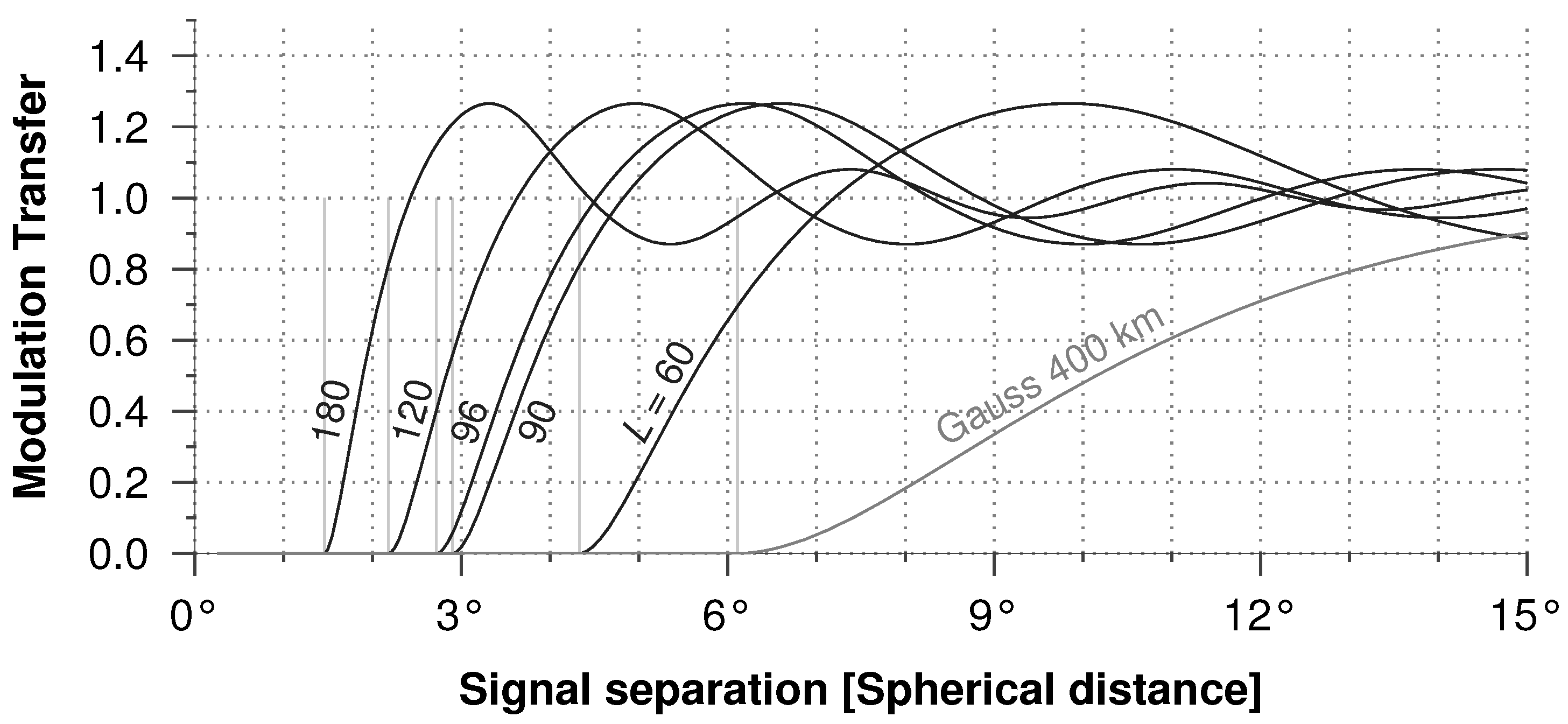
2.2. Ideal Spatial Resolution
2.3. Catchment Averages, Post-Filtering Corrections and Resolution
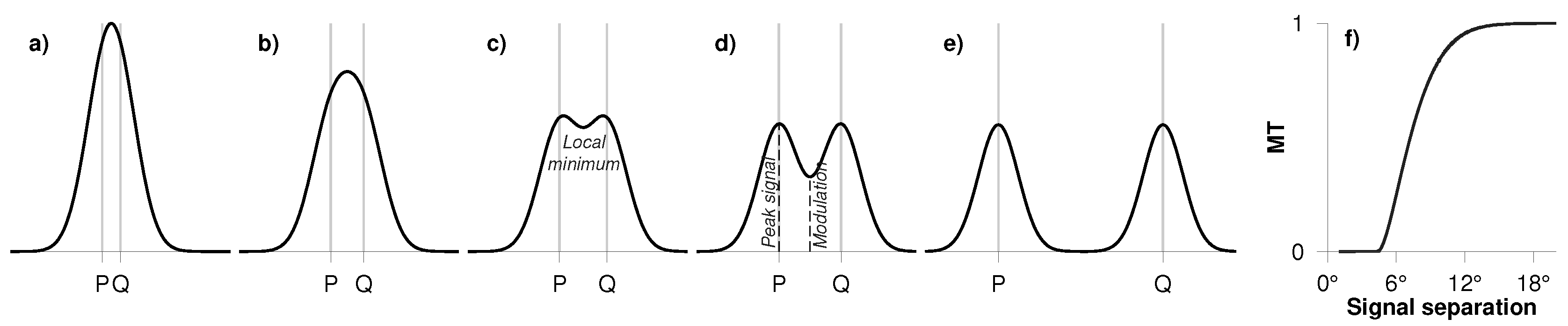
2.4. Some Exceptions
- 1.
- that have a strong seasonal variation in their water storage [7], or
- 2.
- that are similar in magnitude and temporal phase as their neighboring catchments, i.e., without spatial contrast [23] (it should not be confused with the signal contrast/modulation mentioned earlier), or
- 3.
- that are isolated or dominant in terms of their signal strength, for example huge reservoir volume changes [41]
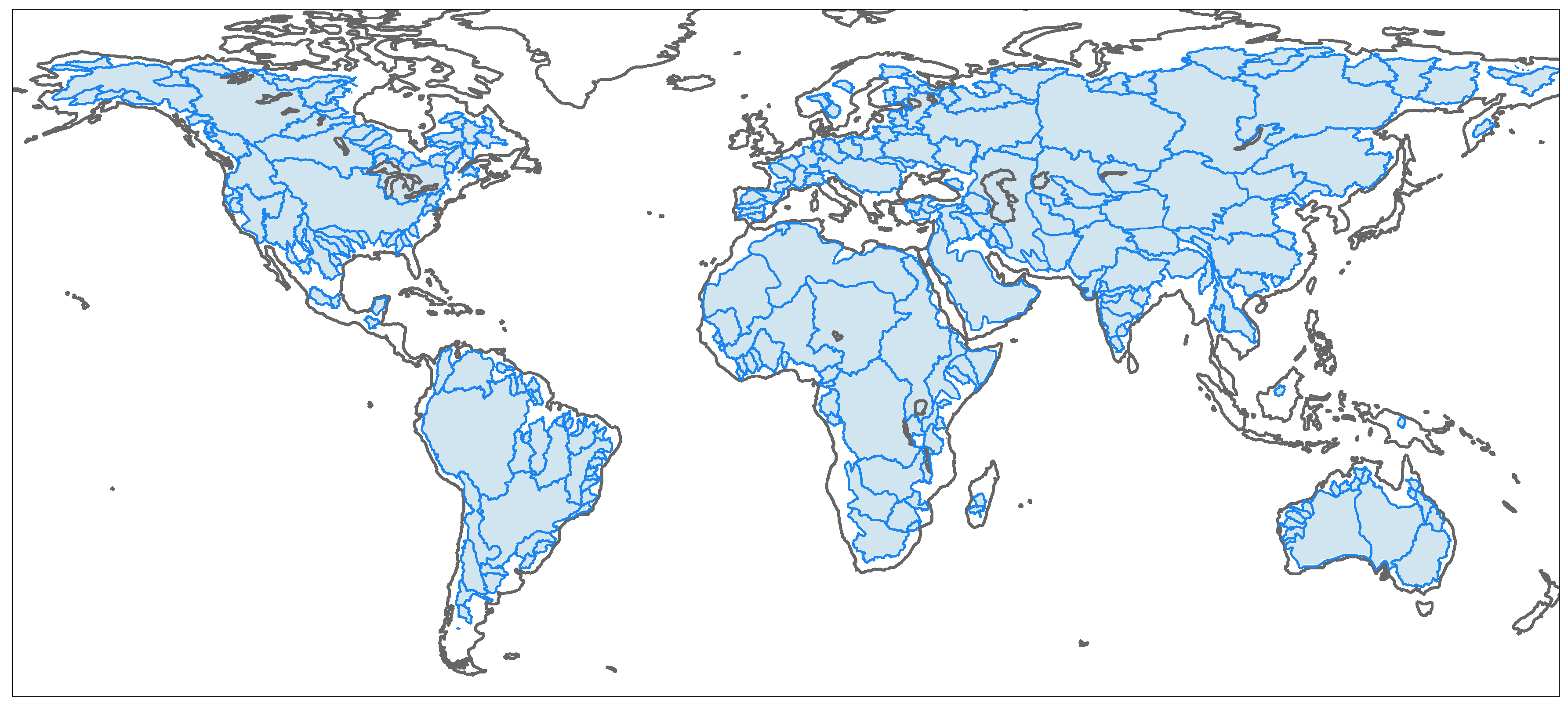
3. Data and Method
| Multiplicative: | [19] | |
| Additive: | [20] | |
| Scaling: | [24] | |
| Data-driven: | [25]. |
- Root Mean Square of Error (RMSE):
- Cyclostationary Nash–Sutcliffe Efficiency () [45,46]:where represents the true value obtained from gldas fields, is the mean annual behaviour (mean monthly values) and m is the number of epochs. RMSE can attain any positive value, a RMSE close to zero represents excellent agreement between and . can attain any value between and 1. A positive value indicates that the difference between the true signal () and the corrected time-series () is well below the non-seasonal variations in the time-series. Typically, hydrological signals have a clear seasonal signal, i.e., change in the amplitude and/or sign of the signal from the summer months to the winter months. However, every summer/winter is not the same and there is a random variation in the amplitude of the signal from year-to-year, which is the non-seasonal variation (the natural variability of the signal). When the error in corrected time-series is smaller than this natural variability, then we can conclude that the signal is very well restored. If we were to use the as proposed by Nash and Sutcliffe [47], without accounting for the cyclostationary seasonal signal, the differences will be compared to the amplitudes of the annual signal. This will not provide a proper indicator for the efficacy of the repairing schemes.
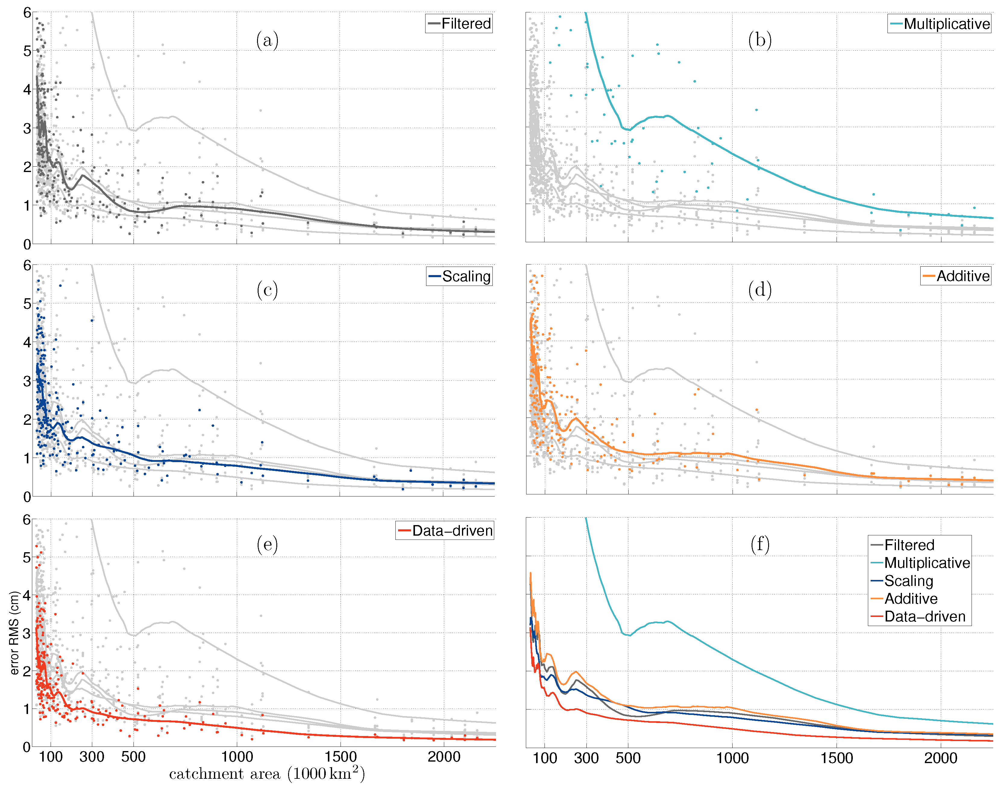
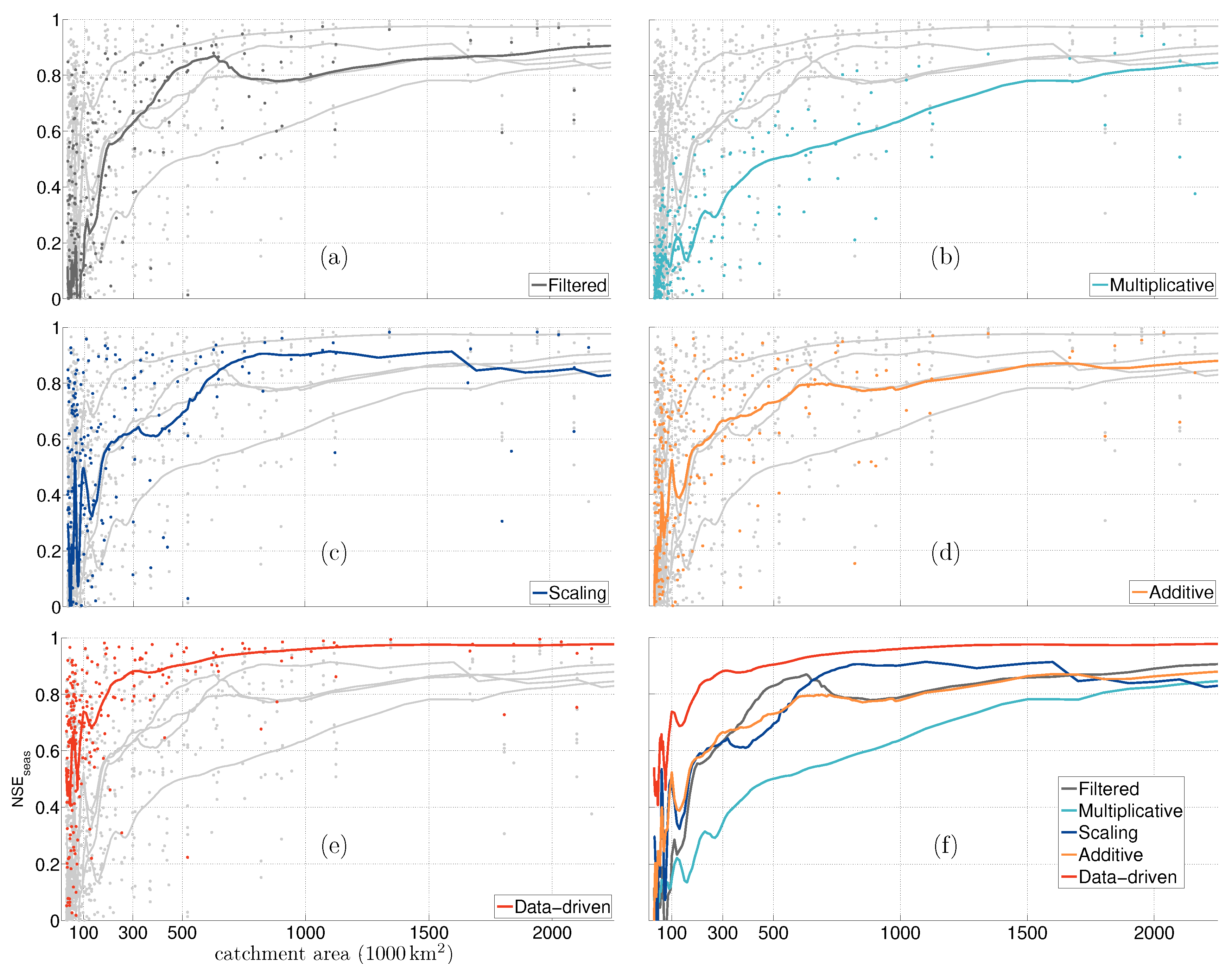
4. Results and Discussion
5. Conclusions
- 1.
- The spatial resolution of the band-limited grace spherical harmonics is not the half-wavelength at the equator, but the ideal spatial resolution. The spatial resolution of filtered grace data can also be described by the ideal spatial resolution.
- 2.
- The users have to be wary that the spatial resolution of the corrected dataset is dependent on the adopted method. Furthermore, the spatial resolution is associated with the error tolerance required by the application and it has to be defined by the user.
- 3.
- Given the fact that with enhanced processing techniques grace is able to see some catchments smaller than the spatial resolution and many catchments close to the band-limit resolution, it is worthwhile to provide spherical harmonics up to a maximum degree of 120 or higher.
Author Contributions
Acknowledgments
Conflicts of Interest
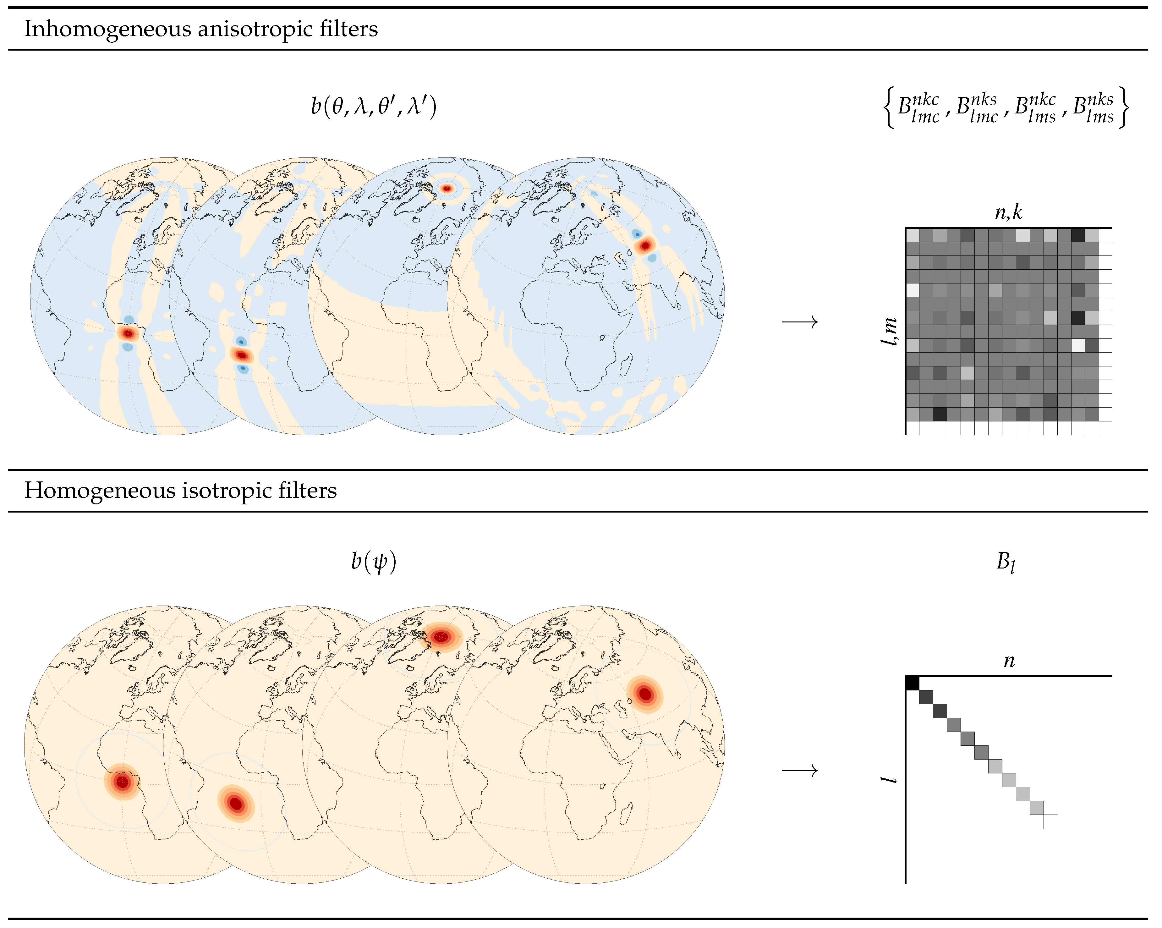
Appendix A. Filtering on the Sphere

References
- Famiglietti, J.S. The global groundwater crisis. Nat. Clim. Chang. 2014, 4, 945–948. [Google Scholar] [CrossRef]
- Sneeuw, N.; Lorenz, C.; Devaraju, B.; Tourian, M.J.; Riegger, J.; Kunstmann, H.; Bárdossy, A. Estimating Runoff Using Hydro-Geodetic Approaches. Surv. Geophys. 2014, 35, 1333–1359. [Google Scholar] [CrossRef]
- Dahle, C.; Flechtner, F.; Gruber, C.; König, D.; König, R.; Michalak, G.; Neumayer, K.H. GFZ GRACE Level-2 Processing Standards Document for Level-2 Product Release 05; Scientific Technical Report-Data 12/02; GFZ: Potsdam, Germany, 2012. [Google Scholar]
- Mayer-Gürr, T.; Behzadpour, S.; Ellmer, M.; Kvas, A.; Klinger, B.; Zehentner, N. ITSG-Grace2016—Monthly and Daily Gravity Field Solutions from GRACE. Website, GFZ Data Services, 2016. Available online: https://www.tugraz.at/institute/ifg/downloads/gravity-field-models/itsg-grace2016/ (accessed on 30 April 2017).
- Swenson, S. Methods for inferring regional surface-mass anomalies from Gravity Recovery and Climate Experiment (GRACE) measurements of time-variable gravity. J. Geophys. Res. 2002, 107, 2193. [Google Scholar] [CrossRef]
- Wahr, J.; Swenson, S.; Velicogna, I. Some Hydrological and Cryospheric Applications of GRACE. In Proceedings of the GRACE Science Team Meeting and DFG SPP1257 Symposium, Potsdam, Germany, 15–17 October 2007. [Google Scholar]
- Lorenz, C.; Devaraju, B.; Tourian, M.J.; Sneeuw, N.; Riegger, J.; Kunstmann, H. Large-scale runoff from landmasses: A global assessment of the closure of the hydrological and atmospheric water balances. J. Hydrometeorol. 2014, 15, 2111–2139. [Google Scholar] [CrossRef]
- Wahr, J.; Molenaar, M.; Bryan, F. Time variability of the Earth’s gravity field: Hydrological and oceanic effects and their possible detection using GRACE. J. Geophys. Res. 1998, 103, 30205. [Google Scholar] [CrossRef]
- Han, S.C.; Shum, C.K.; Jekeli, C.; Kuo, C.Y.; Wilson, C.; Seo, K.W. Non-isotropic filtering of GRACE temporal gravity for geophysical signal enhancement. Geophys. J. Int. 2005, 163, 18–25. [Google Scholar] [CrossRef]
- Swenson, S.; Wahr, J. Post-processing removal of correlated errors in GRACE data. Geophys. Res. Lett. 2006, 33, L08402. [Google Scholar] [CrossRef]
- Kusche, J. Approximate decorrelation and non-isotropic smoothing of time-variable GRACE-type gravity field models. J. Geod. 2007, 81, 733–749. [Google Scholar] [CrossRef]
- Klees, R.; Revtova, E.A.; Gunter, B.C.; Ditmar, P.; Oudman, E.; Winsemius, H.C.; Savenije, H.H.G. The design of an optimal filter for monthly GRACE gravity models. Geophys. J. Int. 2008, 175, 417–432. [Google Scholar] [CrossRef]
- Zhang, Z.Z.; Chao, B.F.; Lu, Y.; Hsu, H.T. An effective filtering for GRACE time-variable gravity: Fan filter. Geophys. Res. Lett. 2009, 36, L17311. [Google Scholar] [CrossRef]
- Devaraju, B. Understanding Filtering on the Sphere—Experiences from Filtering GRACE Data. Ph.D. Thesis, Universität Stuttgart, Stuttgart, Germany, 2015. [Google Scholar]
- Werth, S.; Güntner, A.; Schmidt, R.; Kusche, J. Evaluation of GRACE filter tools from a hydrological perspective. Geophys. J. Int. 2009, 179, 1499–1515. [Google Scholar] [CrossRef]
- Klees, R.; Liu, X.; Wittwer, T.; Gunter, B.C.; Revtova, E.A.; Tenzer, R.; Ditmar, P.; Winsemius, H.C.; Savenije, H.H.G. A Comparison of Global and Regional GRACE Models for Land Hydrology. Surv. Geophys. 2008, 29, 335–359. [Google Scholar] [CrossRef]
- Devaraju, B.; Sneeuw, N. On the Spatial Resolution of Homogeneous Isotropic Filters on the Sphere. In Proceedings of the VIII Hotine-Marussi Symposium on Mathematical Geodesy, Rome, Italy, 17–21 June 2013; Sneeuw, N., Novák, P., Crespi, M., Sansò, F., Eds.; Springer: Cham, Switzerland, 2016; pp. 67–73. [Google Scholar]
- King, M.; Moore, P.; Clarke, P.; Lavallée, D. Choice of optimal averaging radii for temporal GRACE gravity solutions, a comparison with GPS and satellite altimetry. Geophys. J. Int. 2006, 166, 1–11. [Google Scholar] [CrossRef]
- Longuevergne, L.; Scanlon, B.R.; Wilson, C.R. GRACE Hydrological estimates for small basins: Evaluating processing approaches on the High Plains Aquifer, USA. Water Resour. Res. 2010, 46, W11517. [Google Scholar] [CrossRef]
- Klees, R.; Zapreeva, E.A.; Winsemius, H.C.; Savenije, H.H.G. The bias in GRACE estimates of continental water storage variations. Hydrol. Earth Syst. Sci. 2007, 11, 1227–1241. [Google Scholar] [CrossRef]
- Vishwakarma, B.D.; Devaraju, B.; Sneeuw, N. Minimizing the effects of filtering on catchment scale GRACE solutions. Water Resour. Res. 2016, 52, 5868–5890. [Google Scholar] [CrossRef]
- Long, D.; Longuevergne, L.; Scanlon, B.R. Global analysis of approaches for deriving total water storage changes from GRACE satellites. Water Resour. Res. 2015, 51, 2574–2594. [Google Scholar] [CrossRef]
- Vishwakarma, B.D. Understanding and Repairing the Signal Damage Due to Filtering of Mass Change Estimates from the GRACE Satellite Mission. Ph.D. Thesis, University of Stuttgart, Stuttgart, Germany, 2017. [Google Scholar]
- Landerer, F.W.; Swenson, S.C. Accuracy of scaled GRACE terrestrial water storage estimates. Water Resour. Res. 2012, 48, W04531. [Google Scholar] [CrossRef]
- Vishwakarma, B.D.; Horwath, M.; Devaraju, B.; Groh, A.; Sneeuw, N. A Data-Driven Approach for Repairing the Hydrological Catchment Signal Damage Due to Filtering of GRACE Products. Water Resour. Res. 2017, 53, 9824–9844. [Google Scholar] [CrossRef]
- Horwath, M.; Dietrich, R. Signal and error in mass change inferences from GRACE: The case of Antarctica. Geophys. J. Int. 2009, 177, 849–864. [Google Scholar] [CrossRef]
- Baur, O.; Kuhn, M.; Featherstone, W.E. GRACE-derived ice-mass variations over Greenland by accounting for leakage effects. J. Geophys. Res. Solid Earth 2009, 114, B06407. [Google Scholar] [CrossRef]
- King, A.M.; Bingham, J.R.; Moore, P.; Whitehouse, L.P.; Bentley, J.M.; Milne, A.G. Lower satellite-gravimetry estimates of Antarctic sea-level contribution. Nature 2012, 491, 586–589. [Google Scholar] [CrossRef] [PubMed]
- Chen, J.L.; Wilson, C.R.; Li, J.; Zhang, Z. Reducing leakage error in GRACE-observed long-term ice mass change: A case study in West Antarctica. J. Geod. 2015, 89, 925–940. [Google Scholar] [CrossRef]
- Schmidt, R.; Flechtner, F.; Meyer, U.; Neumayer, K.H.; Dahle, C.; König, R.; Kusche, J. Hydrological Signals Observed by the GRACE Satellites. Surv. Geophys. 2008, 29, 319–334. [Google Scholar] [CrossRef]
- Rowlands, D.D.; Luthcke, S.B.; Klosko, S.M.; Lemoine, F.G.R.; Chinn, D.S.; McCarthy, J.J.; Cox, C.M.; Anderson, O.B. Resolving mass flux at high spatial and temporal resolution using GRACE intersatellite measurements. Geophys. Res. Lett. 2005, 32, L04310. [Google Scholar] [CrossRef]
- Tourian, M.; Elmi, O.; Chen, Q.; Devaraju, B.; Roohi, S.; Sneeuw, N. A spaceborne multisensor approach to monitor the desiccation of Lake Urmia in Iran. Remote Sens. Environ. 2015, 156, 349–360. [Google Scholar] [CrossRef]
- Khaki, M.; Forootan, E.; Kuhn, M.; Awange, J.; Longuevergne, L.; Wada, Y. Efficient basin scale filtering of GRACE satellite products. Remote Sens. Environ. 2018, 204, 76–93. [Google Scholar] [CrossRef]
- Heiskanen, W.A.; Moritz, H. Physical Geodesy; W. H. Freeman and Company: San Francisco, CA, USA, 1967. [Google Scholar]
- Weigelt, M.; Sneeuw, N.; Schrama, E.J.O.; Visser, P.N.A.M. An improved sampling rule for mapping geopotential functions of a planet from a near polar orbit. J. Geod. 2013, 87, 127–142. [Google Scholar] [CrossRef]
- Colombo, O.L. Numerical Methods for Harmonic Analysis on the Sphere; Technical Report 310; Department of Geodetic Science, The Ohio State University: Columbus, OH, USA, 1981. [Google Scholar]
- Sneeuw, N. Global spherical harmonic analysis by least squares and numerical quadrature methods in historical perspective. Geophys. J. Int. 1994, 118, 707–716. [Google Scholar] [CrossRef]
- McEwen, J.D.; Wiaux, Y. A Novel Sampling Theorem on the Sphere. IEEE Trans. Signal Process. 2011, 59, 5876–5887. [Google Scholar] [CrossRef]
- Freeden, W.; Schreiner, M. Spherical functions of mathematical geosciences. In Advances in Geophysical and Environmental Mechanics and Mathematics; Springer: Berlin, Germany, 2009; p. 602. [Google Scholar]
- Jekeli, C. Alternative Methods to Smooth the Earth’s Gravity Field; Technical Report 327; Department of Geodetic Science and Surveying, The Ohio State University: Columbus, OH, USA, 1981. [Google Scholar]
- Yi, S.; Song, C.; Wang, Q.; Wang, L.; Heki, K.; Sun, W. The potential of GRACE gravimetry to detect the heavy rainfall-induced impoundment of a small reservoir in the upper Yellow River. Water Resour. Res. 2017, 53, 6562–6578. [Google Scholar] [CrossRef]
- Rodell, M.; Houser, P.R.; Jambor, U.; Gottschalck, J.; Mitchell, K.; Meng, C.J.; Arsenault, P.R.; Cosgrove, B.; Radakovich, J.; Bosilovich, M.; et al. The Global Land Data Assimilation System. Bull. Am. Meteorol. Soc. 2004, 85, 381–394. [Google Scholar] [CrossRef]
- Werth, S. Calibration of the Global Hydrological Model WGHM with Water Mass Variations from GRACE Gravity Data. Ph.D. Thesis, Universität Potsdam, Potsdam, Germany, 2010. [Google Scholar]
- Döll, P.; Müller Schmied, H.; Schuh, C.; Portmann, F.T.; Eicker, A. Global-scale assessment of groundwater depletion and related groundwater abstractions: Combining hydrological modeling with information from well observations and GRACE satellites. Water Resour. Res. 2014, 50, 5698–5720. [Google Scholar] [CrossRef]
- Thor, R. Least-Squares Prediction of Runoff. Bachelor’s Thesis, University of Stuttgart, Stuttgart, Germany, 2013. [Google Scholar]
- Lorenz, C.; Tourian, M.J.; Devaraju, B.; Sneeuw, N.; Kunstmann, H. Basin-scale runoff prediction: An Ensemble Kalman Filter framework based on global hydrometeorological data sets. Water Resour. Res. 2015, 51, 8450–8475. [Google Scholar] [CrossRef]
- Nash, J.E.; Sutcliffe, J.V. River flow forecasting through conceptual models part I—A discussion of principles. J. Hydrol. 1970, 10, 282–290. [Google Scholar] [CrossRef]
- Cleveland, R.; Cleveland, W.; McRae, J.; Terpenning, I. STL: A Seasonal-Trend Decomposition Procedure Based on Loess (with Discussion). J. Off. Stat. 1990, 6, 3–73. [Google Scholar]
- Flechtner, F.; Neumayer, K.H.; Dahle, C.; Dobslaw, H.; Fagiolini, E.; Raimondo, J.C.; Güntner, A. What Can be Expected from the GRACE-FO Laser Ranging Interferometer for Earth Science Applications? Surv. Geophys. 2016, 37, 453–470. [Google Scholar] [CrossRef]
- Rummel, R.; Schwarz, K.P. On the nonhomogeneity of the global covariance function. Bull. Geod. 1977, 51, 93–103. [Google Scholar] [CrossRef]


| L | Half-Wavelength | Ideal Spatial Resolution | |||||
|---|---|---|---|---|---|---|---|
| [1000 km] | [km] | [1000 km] | [km] | ||||
| 60 | 3 | 111.5 | 334 | 182.4 | 427 | ||
| 90 | 2 | 49.6 | 223 | 81.9 | 286 | ||
| 96 | 1 | 43.6 | 209 | 72.0 | 268 | ||
| 120 | 1 | 27.9 | 167 | 46.2 | 215 | ||
| 180 | 1 | 12.4 | 111 | 20.7 | 144 | ||
| Gauss 400 km | n/a | n/a | n/a | 363.2 | 603 | ||
| RMSE () | Filtered | Multiplicative | Additive | Scaling | Data-Driven |
|---|---|---|---|---|---|
| 1 | 750 | 1563 | 1103 | 563 | 250 |
| 1.5 | 337 | 1323 | 360 | 260 | 152 |
| 2 | 152 | 1103 | 152 | 90 | 63 |
| 2.5 | 90 | 951 | 1223 | 76 | N/A |
| 3 | N/A | 810 | N/A | N/A | N/A |
| Filtered | Multiplicative | Additive | Scaling | Data-Driven | |
|---|---|---|---|---|---|
| 0.9 | 2000 | – | – | 750 | 450 |
| 0.8 | 1100 | 1750 | 1100 | 600 | 200 |
| 0.7 | 380 | 1200 | 450 | 500 | 150 |
| 0.6 | 280 | 900 | 250 | 250 | 90 |
| 0.5 | 200 | 480 | 180 | 180 | N/A |
© 2018 by the authors. Licensee MDPI, Basel, Switzerland. This article is an open access article distributed under the terms and conditions of the Creative Commons Attribution (CC BY) license (http://creativecommons.org/licenses/by/4.0/).
Share and Cite
Vishwakarma, B.D.; Devaraju, B.; Sneeuw, N. What Is the Spatial Resolution of grace Satellite Products for Hydrology? Remote Sens. 2018, 10, 852. https://doi.org/10.3390/rs10060852
Vishwakarma BD, Devaraju B, Sneeuw N. What Is the Spatial Resolution of grace Satellite Products for Hydrology? Remote Sensing. 2018; 10(6):852. https://doi.org/10.3390/rs10060852
Chicago/Turabian StyleVishwakarma, Bramha Dutt, Balaji Devaraju, and Nico Sneeuw. 2018. "What Is the Spatial Resolution of grace Satellite Products for Hydrology?" Remote Sensing 10, no. 6: 852. https://doi.org/10.3390/rs10060852
APA StyleVishwakarma, B. D., Devaraju, B., & Sneeuw, N. (2018). What Is the Spatial Resolution of grace Satellite Products for Hydrology? Remote Sensing, 10(6), 852. https://doi.org/10.3390/rs10060852