Abstract
The Nyingchi Mw 6.4 earthquake on 17 November 2017 is the first large event since 1950 at the southeast end of the Jiali fault. This event was captured by interferometric synthetic aperture radar (InSAR) measurements from the European Space Agency (ESA) Sentinel-1A radar satellite, which provide the potential to determine the fault plane, as well as the co-seismic slip distribution, and understand future seismic hazards. However, due to the limited magnitude of surface displacements and the strong topography variations, InSAR-derived co-seismic signals are contaminated by strong tropospheric effects which makes it difficult (if not impossible) to determine the source parameters and co-seismic slip distribution. In this paper, we employ the Generic Atmospheric Correction Online Service for InSAR (GACOS) to generate correction maps for the co-seismic interferograms, and successfully extract co-seismic surface displacements for this large event. The phase standard deviation after correction for a seriously-contaminated interferogram reaches 0.8 cm, significantly improved from the traditional phase correlation analysis (1.13 cm) or bilinear interpolation (1.28 cm) methods. Our best model suggests that the seismogenic fault is a NW–SE striking back-thrust fault with a right-lateral strike slip component. This reflects the strain partitioning of NE shortening and eastward movement of the Eastern Tibetan plateau due to the oblique convergence between the Indian and Eurasian plates.
1. Introduction
On 17 November 2017, a Mw 6.4 earthquake hit the Tibetan plateau, 63 km northeast of Nyingchi, China (Figure 1). The epicenter lies on the southeastern edge of the Tibetan plateau where the dominating tectonic movement is driven by the oblique convergence between the Indian and Eurasia plates [1,2,3]. This region has long been characterized as having weak tectonic activity [4,5,6], with a limited number of recorded historical events according to the United States Geological Survey (USGS) and the China Earthquake Administration (CEA). Only a limited number of geodetic surveys have been conducted in this region and this is the first large earthquake that has been captured by one of the modern geodetic techniques, SAR interferometry, with the ESA’s Sentinel-1A radar satellite [7]. These InSAR measurements provide high spatial resolution co-seismic surface displacements, which can be used to infer the source parameters of seismogenic faults, assess future seismic hazards, and better understand the activity of seismogenic structures.
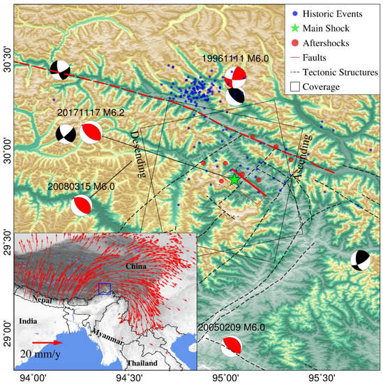
Figure 1.
Tectonic setting for the Mw 6.4 Nyingchi earthquake. Historic earthquakes recorded by the USGS database from January 1950 to October 2017 are plotted as blue dots, the main shock is indicated by a green star and aftershocks by red dots. Historic major events recorded by CEA are plotted by a beach ball (red for Mw > 6.0, and black for Mw < 6.0). The GPS velocity field (red arrows) is referenced from Liang et al. [29]. The event was covered by two pairs of Sentinel-1A images with different geometries (solid line boxes). The red solid line is the modeled fault plane projected on the Earth’s surface.
One of the major sources of error for InSAR is the phase delay in radio signal propagation through the atmosphere (especially the part due to the troposphere), with which only a few centimeters of precision can be reliably achieved for displacement retrievals even under a relatively quiet atmospheric environment [8,9,10,11]. Tropospheric delays are often correlated with topography, but coupled with strong turbulent signals, which makes it difficult to distinguish them from actual tectonic movements [9,12]. While extensively addressed in post- and inter-seismic studies where millimeter-level precision of velocity mapping is needed [8,13,14], tropospheric delays are typically ignored in co-seismic modeling under the hypothesis that the magnitude of co-seismic signals is much greater than that of tropospheric delays [15,16,17,18]. However, for earthquakes with small-magnitude surface displacements, tropospheric delays can be of the same order, or even larger, than ground motions. For example, the Nyingchi earthquake occurred in a high-altitude region with strong topography variations where the co-seismic signals are significantly masked by the elevation-dependent tropospheric delays, which makes it difficult to determine the source parameters and resolve the fault slip distribution. Lee et al. [19] used a stacking method to combine a series of interferograms to minimize tropospheric errors in order to extract small co-seismic signals for three Mw 5.2–5.6 2004 Huntoon Valley earthquakes. However, it required a delayed response to the event and additional data before and after the earthquake, which is usually not available. Fattahi et al. [20] utilized the European Centre for Medium-Range Weather Forecasts Re-Analysis (ERA) Interim global atmospheric model for correcting tropospheric effects for the co-seismic interferograms for the Mw 5.5 Ghazaband earthquake, but only stratified delays were considered. Feng et al. [21] employed the MEdium Resolution Imaging Spectrometer (MERIS) near-IR water vapor data for correcting RADARSAT-2 images for the Mw 8.3 Illapel earthquake, which is claimed to be better than ERA-Interim, but is not available for recent satellite missions, such as Sentinel-1 and ALOS-2 [22]. The abovementioned correction methods have disadvantages because of (i) usually being delayed for 1–3 months from the event; (ii) low spatial or temporal resolution for capturing the tropospheric turbulence; and (iii) incompatibility with newly-launched satellites, such as Sentinel-1 and ALOS-2.
In this paper, we attempt to correct tropospheric effects on Sentinel-1A interferograms using the Generic Atmospheric Correction Online Service for InSAR (GACOS) developed at Newcastle University, which employs the high-resolution weather model outputs from the European Centre for Medium-Range Weather Forecasts (HRES-ECMWF) to generate high-resolution tropospheric delay maps for InSAR atmospheric correction [9,23]. After correction, both ascending and descending interferograms show clearer co-seismic signals than the original ones, which are then used to inverse the optimal fault geometry and co-seismic slip model of the Nyingchi event. The slip model is carefully tested by Monte Carlo and checkerboard tests, after which the coulomb stress changes are calculated to assess local seismic impacts.
2. Tectonic Setting
Driven by the northward movement of the Indian plate relative to the stable Eurasian plate at a rate of ~4 cm/year [24], the tectonics in Southern Tibet are dominated by a mixture of normal and strike-slip faulting [3,6,25], which is in contrast with the thrust faulting along the ranges bordering the Tibetan plateau [26]. Most of the faults are predominantly south–north striking normal faults, although many locations also show oblique displacement, and reflect the eastward tectonic extrusion mostly during ~18–13 Ma [27,28]. The Karakoram-Jiali strike slip fault system terminates the normal faulting system at its northern tips and releases part of the collision energy. Lee et al. [6] suggest that the Jiali fault was initiated and most active during ~18–12 Ma and is best explained as the accommodation of deformation from oblique convergence between the India and Eurasian plates. Furthermore, the clockwise rotation of the GPS velocity field from NE motion to eastward motion could result in a NE shortening recorded by historical events (Figure 1).
The Mw 6.4 Nyingchi earthquake occurred on a blind fault in the southeast part of the main Jiali fault, where a limited number of historic events have been recorded. From here, the Jiali fault is divided into several north–south striking faults, such as the Puqu and Kumon faults. One Ms 6.0 strike slip earthquake happened on 11 November 1996 on the north side of the Jiali fault, and another Ms 6.0 event happened on 15 March 2008 on the south side, but with more thrusting slips. These two events were not recorded by the USGS. Most of the historic small quakes (<Mw 6.0) centered on the northern part of the Jiali fault. The aftershocks are randomly distributed and small in magnitude (<Mw 5.0), suggesting a high percentage of stress released from the main shock.
3. Datasets and Error Mitigation
The event is spatial-temporally covered by two pairs of Sentinel-1A interferograms of both descending and ascending geometries (Table 1). We generated the interferograms with the GAMMA software [30], developed by the corporation of Aktiengesellschaft in Bern of Switzerland, using precise orbits from [31]. Topographic phase contributions were removed using a 1-arcsec (~30 m) SRTM digital elevation model [32], and topographic errors were considered negligible due to the short spatial baselines (Table 1).

Table 1.
Sentinel-1A interferograms used for co-seismic modeling and atmospheric correction results.
Clear atmospheric effects can be observed in Figure 2, especially in mountain areas. For the descending interferogram, the co-seismic signals are significantly masked by atmospheric delays, which makes it difficult to check the ground motion patterns. The comparable magnitude of atmospheric delays and co-seismic signals decreases the signal-to-noise ratios and, in turn, leads to unreasonable down-sampling points for modeling. These errors can be largely avoided when dealing with medium to large earthquakes with strong ground motion (as the signal-to-noise ratio is high), but become vital when modeling small and/or deeply-buried earthquakes with small surface displacements.
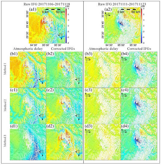
Figure 2.
InSAR observations and atmospheric corrections. (a1,a2) are raw interferograms. Method 1 (b1–b4) is HRES-ECMWF interpolated by the ITD model. Method 2 (c1–c4) removes signals correlated with elevation. Method 3 (d1–d4) is HRES-ECMWF interpolated bilinearly. Note the coverage is different from Figure 1 as the very far field data has been cut.
To overcome this, we introduced the operational HRES-ECMWF product, incorporating modeled surface pressure, temperature, and specific humidity, to calculate tropospheric delays at each 0.125-degree grid point (i.e., spacing of approximately 9–12 km) spatially and 6 h temporally [11]. A simple linear temporal interpolation is applied as the acquisition time of the SAR images and HRES-ECMWF data are not identical. In order to properly mitigate the topographic-related tropospheric delays, we applied an iterative tropospheric decomposition (ITD) model [23], which separates the tropospheric turbulence and elevation dependent signals through iteration due to their different behaviors, and reduces their coupling effect. The total delays in ITD are described as:
where, for the ZTD at location k, T represents the turbulent component and xk is the station coordinate vector in the local topocentric coordinate system; (L0, β) are the coefficients of the exponential function for the stratified component; h is the altitude; and ε represents the remaining unmodeled errors. The detailed procedures of ITD are: (i) For each map pixel, the surrounding ZTDs from all HRES-ECMWF nodes are used to estimate the initial values for the exponential coefficients, assuming the turbulent components are zero; (ii) The residuals after step (i) are used to estimate the turbulent part by inverse distance weighting (IDW). Those components not obeying the IDW are treated as unmodeled errors; (iii) Subtract the turbulent component estimated by step (ii) from the total delays and re-estimate the exponential coefficients; (iv) Repeat steps (ii) to (iii) until the exponential coefficients are converged. The ZTD for the pixel considered is then obtained by interpolating the turbulent components and unmodeled errors from all HRES-ECMWF nodes, and added to the stratified delay computed using the final values of the exponential coefficients for the pixel considered.
Yu et al. [23] pointed out that the iterative separation produces smaller RMS in mountain areas or more turbulent atmospheres compared to the traditional models without iteration and, therefore, is valuable to this study as the main co-seismic displacements occurred on a high altitude mountain (over 3 km) and the elevation-dependent signal is dominating. Tropospheric corrections for each pixel of the interferograms are then interpolated from the ECMWF grids by ITD and projected to line of sight (LOS), and the corrected interferograms are then obtained (Figure 2). It is clear that the co-seismic signals stand out in the corrected interferograms with two major lobes.
To validate the ITD performance, we also presented the results of (i) the conventional removal of signals correlated with altitude. This was done by fitting the observed phase (excluding near field observations) to an exponential function: phase = a × exp(b × h), a and b are coefficients, and h is the altitude. Phases correlated with altitude are removed after estimating the coefficients; and (ii) a simple bilinear interpolation of the HRES-ECMWF data.
It is clear that ITD presents the best performance, especially for the pair from 6 November 2017–18 November 2017, as its atmosphere contamination is more serious. The simple bilinear interpolation performs the worst since the elevation dependency of the tropospheric delay is not considered and the HRES-ECMWF data was over-interpreted at some large topography variation areas (e.g., the valley in the southeast of Figure 2(d1)). Although the atmospheric contaminations in Figure 2a have some correlations with topography, these correlations could have very localized characters and are difficult to describe by one equation. The phase-elevation correlation can be shifted due to water vapor flow [33] so that the peak delay values do not necessarily occur on the peak altitudes. Furthermore, the conventional removal of elevation-dependent signals has large potentials of removing actual ground displacements. When the atmospheric contamination is limited, such as on the pair from 11 November 2017–23 November 2017, all methods perform similarly, but we still see more improvements from ITD on the northeast and southwest areas. See Table 1 for lists of the statistics of the three methods.
To further assess the reliability of the GACOS corrections, we calculated the correlations between the observed phase observations and the GACOS-derived tropospheric delays for all pixels. When tropospheric delays dominate an interferogram, the observed phase pattern should be similar to the tropospheric delay maps, especially for the long-wavelength signals. A high correlation is found for the descending interferogram in Figure 3a, suggesting that GACOS is able to capture most of the atmospheric effects, and the atmospheric correction is successful in this case. The smaller magnitude of the tropospheric delays for the ascending interferogram produces a lower correlation. The phase standard deviation (StdDev) after correction (excluding the near field co-seismic region) indicates the phase flatness and should be small when no strong ground movement happened, as is the case for the far field region. Other uncertainties could be introduced by the large time difference between the InSAR and HRES-ECMWF acquisitions or the large topographic variations. The descending track shares smaller time differences and higher phase-delay correlation, thus producing smaller phase StdDev and higher correction performance. Although the time difference is higher for the ascending track, the overall magnitude of the tropospheric delay is small (see Figure 3b) and can be considered negligible after correction. All these statistics demonstrate a successful tropospheric correction and ensure a high precision of the corrected data, which has clearer co-seismic displacements and a higher signal-to-noise ratio and, therefore, more applicable in the next modelling step.
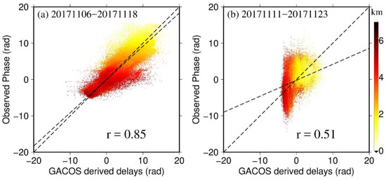
Figure 3.
Correlations between the observed phase and the modeled tropospheric corrections for the descending (a) and ascending (b) tracks, respectively. Each dot represents one pixel of the interferograms, the color scale corresponds to its elevation, and r is the correlation ratio.
4. Co-Seismic Modelling and Results
The corrected interferograms were down-sampled using a quadtree quantization algorithm: pixels with coherence smaller than 0.4 were excluded to reduce the high spatial correlation and computation burden. This led to 1345 samples for the descending track and 1947 for the ascending track for input into the model.
The modelling is implemented in two steps. The first is the determination of the fault geometry by minimizing the square misfit, under an assumption of a uniform slip on a rectangular fault in a homogeneous elastic half-space [34]. An improved particle swarm optimization [35] is utilized to solve the non-linear equations, and a downhill simplex method [36] is employed to further search for the preferred solution. This is determined through a histogram analysis to avoid the convergence at a local minimum, which is crucial for this event as the signal-to-noise ratio is low.
The second step is to linearly resolve the slip distribution by constructing a 15 km × 25 km fault plane and discretize it into 0.5 km × 0.5 km patches. For each fault segment, we hold its striking angle fixed from the previous step and estimate the striking and dip slips. We use ABIC to search for the smoothing factor and dip angle simultaneously. The optimal values are found by minimizing the ABIC function:[37]:
where α2 is the smoothing factor; δ is the dip angle; p is the probability density function; a is the fault slip factors; d is the observation vector; and C is the constant that is not related to the smoothing factor and the dip angle. For detailed equations related to ABIC, please refer to [37].
The best-fitting fault geometry parameters are 132.8° strike and 59° dip. The optimal rake angle is 115° which indicates a combination of right-lateral strike and reverse dip slips. The resolved fault depth is 9 km, which indicates a total moment of 4.84 × 10¹⁸ Nm, corresponding to a magnitude of Mw 6.4. Our preferred model suggests a larger dip angle of 59° than the USGS 36° and a larger rake of 115° than the USGS 95° solution. However, our slip distribution model allows the fault slips to vary from 80° to 115°. The overall explained ratios (defined as (1-abs(residual)/observation) for the near field deforming area) are, respectively, 78% and 82% for the descending and ascending interferograms, which corresponds to a misfit RMS of 1.12 and 0.95 cm. We performed a Monte Carlo test for estimating the uncertainties and trade-offs of the fault geometry parameters based on the method described in [38]. We used the far field observations to construct an approximate variance-covariance matrix (VCM) and then generated 100 perturbed datasets to solve for a set of 100 model solutions. The distribution of values of each model parameter from the Monte Carlo test (see Section 4) are plotted in Figure 4 as a histogram, and used to estimate the uncertainty in that parameter, and plotted against each other and, therefore, used to qualitatively assess the trade-offs between those parameters. Most of the parameters are well-resolved, appearing as tight clusters in the scatterplots and narrow peaks in the histograms. The overall uncertainties are considered small, which offers a good confidence of the non-linear estimation. Figure 5d showed that the fault dip can be well-determined from the two tracks of InSAR observations, which is also evidenced from the following checkboard test. On the other hand, the smoothing factor does not significantly affect the data misfit for this small event. The residuals on the descending interferogram are likely due to the combined contribution of interferometric decorrelation in the near field and the remaining atmospheric delays.
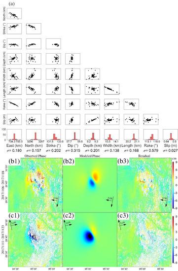
Figure 4.
(a) Uncertainty analysis by Monte Carlo testing for the nonlinear inversion: standard deviation (red histograms) and trade-offs (scatter plots) between the model parameters. The vertical axes of the first column share the same scale with the bottom horizontal axes. The rest are observed observations (b1,c1), modeled displacement (b2,c2), and residuals (b3,c3).
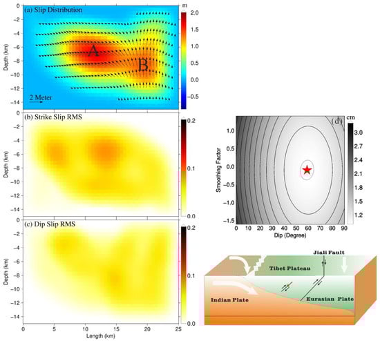
Figure 5.
Fault plane slip distribution of the Nyingchi M6.4 earthquake; (a–c) are the slip RMS values by Monte Carlo testing along the strike and dip directions, respectively; (d) is the contour map of ABIC searching for the optimal smoothing factor and fault dip. The smoothing factor is represented as log(α2) in Equation (1). The color bar indicates the data misfit RMS. The determined optimal values are 0.9 for α2, and 59 for dip angle. The fault geometry is also illustrated with reference to the Jiali fault [6] and the Indian and Eurasian Plates.
The fault plane slip distribution in Figure 5 is divided into two regions. Region A is characterized as mostly right lateral strike slips with a rake angle of ~115° and a maximum of slip of 1.9 m. The slips are concentrated at depths of 5 to 11 km with a maximum at 8 km. Region B is nearly a pure dip slip and of smaller magnitude compared to A. The dip slips are deeper with a maximum occurring at 10 km. The hypocenter is located at the west side of the fault plane, which indicates that the fault rupture propagates from west to east, and from right-lateral to reverse faulting. The fault slips along the strike for a distance of 25 km with a varying slip magnitude from 0.3 m to 1.9 m and on the fault patches at a depth of 5–12 km. The transition from the strike slip in the west to the dip slip in the east reflects well the oblique convergence of the Indian plate. This movement is consistent with the local topography which has high mountains on the hanging wall, but relatively lower on the footwall. In this region, the Tibetan plateau is pushing out eastwards, resulting in an E–W extension which may be evidenced by the strike slip Jiali fault. The extension and the collision between the Indian and Eurasian plates result in this back-thrust fault.
5. Discussions
The atmospheric correction improves the signal-to-noise ratio of the interferograms and makes the near field displacement stand out, which is beneficial for searching the optimal fault position and strike direction in the non-linear inversion step (see Figure 4). Another key question specifically for modeling the small magnitude earthquake is to determine the fault dip, which is more sensible to far field observations, but more likely to be masked by atmospheric delay due to the smaller displacements, especially when the fault is deeply buried. As we can see from Figure 2, the proposed method reduced most of the elevation-dependent atmospheric error, independently estimated from the weather model, in the far field, especially on the west-side mountain areas of the interferogram, whereas the other two methods still leave a large portion of atmospheric delay residuals due to the steep topographies. Simple interpolation methods or phase correlation analysis are, thus, not satisfactory on this occasion. Similarly, the proposed method can also be applied on larger earthquakes to help improve the far field observations in order to determine the down dip fault slip distributions.
To assess the robustness and resolution of the best-fit solution, we employed two separate error analysis techniques: the Monte Carlo test for fault slip distribution uncertainty analysis and checkerboard tests. Firstly, we used the Monte Carlo method to estimate the uncertainty of our best-fit slip distribution model. It is conducted by perturbing the observations 1000 times with spatial noise as estimated from the previous best-fit solution and then the same parameter is used to search each of these datasets to find the best-fitting slip model [37]. Secondly, to assess the inversion resolution of the fault slips on both shallow and down-dip parts, we generated synthetic data for the checkerboard-like slip distributions, and recovered fault slips from these observations using the same parameters and settings [38]. The Monte Carlo test in Figure 5 suggests the fault slip RMS of 2.8 cm (9.3%) along the strike and 2.3 cm (6.2%) along the dip. Most of the slip discrepancies occurred along the strike are located in accordance with the dominating shallow strike slipping, whereas the downdip slip RMS is small. From the checkerboard test displayed in Figure 6, the input model is nearly fully recovered above ~12 km suggesting a fine slip inverse resolution. Due to the high dip angle, the downdip (below 12 km) slip pattern is poorly recovered, resulting in a lower slip distribution resolution. This is one of the limitations to using ground observations to invert for slip distribution, especially for deeply-buried high-dip earthquakes [39,40].
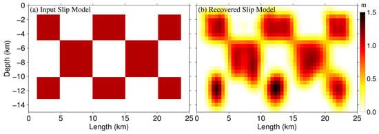
Figure 6.
Checkerboard test for fault slip distribution using the modeled fault geometry and the down-sampled InSAR observation distributions.
We have examined the coulomb stress changes (CSS) in Figure 7 for the main shock as it plays an important role to trigger slips in neighboring seismic zones. The CSS are calculated at 0 and 8 km depths, respectively, based on the fault model with the receiver fault parameters of 132.8° for strike, 59° for dip, 115° for rake, 25 km for length, 15 km for width, and the friction coefficient of 0.4. [41,42]. The near field hanging wall has an increase in CSS at the surface, but a decrease at a depth of 8 km. Most of the accumulated stress of the northwest part of the fault at a depth of 8 km is released with a spreading CSS lobe to the west far field (Figure 7b). However, the southeast end of the fault has a wide spread CSS increasing the lobe at 8 km, suggesting a stress accumulation on its surroundings. The main shock has triggered the inactive Jiali fault to slip and produce several small aftershocks.
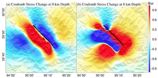
Figure 7.
Coulomb stress changes of the Nyingchi Mw 6.4 earthquake calculated by the optimal fault plane slip distribution at the surface and at a depth of 8 km.
The oblique convergence between the Indian and Eurasian plates results in a wide shear zone and rocks are intensely folded and faulted parallel to the shear zone with the main steeply-dipping right lateral strike slip Jiali fault [6]. The Jiali fault was most active during ~18–12 Ma, but less active since then with limited large events occurring. The Nyingchi Mw 6.4 earthquake is the most powerful event ever recorded in this region since 1950 and the modeled surface movements suggest it released at least part of the cumulated stress induced by the background Indian-Eurasia tectonic motion. The modeled surface fault trace is parallel to the Jiali fault with a small bias to the northeast. Most of the surface displacements are concentrated on the hanging wall (southwest of the fault trace) which reflects the NE shortening of the clockwise rotation of the GPS velocity from NNE to NEE in the Eastern Tibetan plateau (Figure 1) given the fact that the driven force mainly comes from the northward movement of the Indian plate relative to the stable Eurasian plate at a rate of ~4 cm/year.
6. Conclusions
In this paper, we inverted the fault geometry and modeled the slip distribution of the Nyingchi earthquake using InSAR observations. This is the first time in this region that a large event (>Mw 6.0) was captured by a modern geodetic technique, providing valuable information on the local faulting system and tectonic strain balance induced by the oblique convergence between the Indian and Eurasian plates over Southeast Tibet. The major contributions of this paper are to (i) introduce a generic atmospheric correction model dealing with both the stratified and turbulent tropospheric contaminations, thus increasing the InSAR capability for measuring small-magnitude earthquakes in near real-time; (ii) map the buried fault geometry located south of the Jiali fault in Tibet using InSAR measurements for the first time; and (iii) provide evidence from the modeled fault plane slip distribution for the oblique convergence of the Indian-Eurasian plates.
We have shown the ability of using Sentinel-1A interferograms for mapping the Nyingchi Mw 6.4 earthquake with small ground displacements, but strong atmospheric effects, by using the GACOS atmospheric corrections. The correction model largely reduced the tropospheric contamination without masking the actual ground motion, especially the elevation-dependent delays, which is important for steep topographic areas, as is the case for most tectonically-active regions. After correction, the phase StdDev improved from 1.83 to 0.73 cm for the descending track and 1.47 to 0.8 cm for the ascending track, which is superior to the phase correlation analysis method by removing an elevation-correlated component (1.13 and 0.93 cm after correction for the two orbits) and a simple bilinear interpolation method (1.28 and 0.99 cm after correction for the two orbits). The co-seismic signal stood out only after the GACOS correction and the far field observations were cleaned, which improved the inversion of downdip fault slips. The same correction procedure can also be applied to post-/inter-seismic subsidence in urban areas and landslide monitoring.
The fault geometry and slip distribution were inverted using the corrected interferograms and a mixture of right lateral and reverse slip was found. The maximum slip on the determined fault is 1.9 m and concentrated in the northwest part of the fault plane at a depth of 8 km. The slip model reflects well the east–west extension of the Tibetan plateau, as well as the convergence of the Indian to the stable Eurasia plate. Few aftershocks were recorded, suggesting a large portion of the stress has been released by the main shock. The major Jiali fault in this region was probably triggered by the main shock and produced several small aftershocks along its strike direction.
Since our method is globally available in near real-time, it can also be applied to larger earthquakes and other InSAR applications, such as volcanic events, post/inter-seismic studies, landslides, and city subsidence. All these applications encountered serious tropospheric contamination and the error magnitude increases as the study area extends. Successful usage of our proposed method will help to reduce the elevation-dependent tropospheric signals, as well as the turbulence component, as discussed in Equation (1). The proposed method has been made available from our website (http://ceg-research.ncl.ac.uk/v2/gacos/) and provides high-resolution InSAR tropospheric correction maps globally in near real-time which can be directly applied on interferograms in the same way as proposed in this paper. The correction maps are suitable for all SAR satellites as the tropospheric delay is independent from the signal wavelength.
In the near future we plan to include the tropospheric correction procedure in an automatic processing chain for monitoring tectonic motions and rapid earthquake response system.
Author Contributions
C.Y. and Z.L. conceived and designed the experiments; C.Y. and J.C. performed the experiments; C.Y., J.-C.H., and Z.L. analyzed the data; C.Y. wrote the paper; and all the co-authors contributed to the writing.
Acknowledgments
This work was supported by a Chinese Scholarship Council studentship awarded to Chen Yu (ref. 201506270155). Part of this work was also supported by the UK NERC through the Centre for the Observation and Modelling of Earthquakes, Volcanoes, and Tectonics (COMET, ref.: come30001), the LICS and CEDRRIC projects (ref. NE/K010794/1 and NE/N012151/1, respectively), and the ESA-MOST DRAGON-4 project (ref. 32244).
Conflicts of Interest
The authors declare no conflict of interest.
References
- Yin, A.; Harrison, T.M. Geologic Evolution of the Himalayan-Tibetan Orogen. Annu. Rev. Earth Planet. Sci. 2000, 28, 211–280. [Google Scholar] [CrossRef]
- Armijo, R.; Tapponnier, P.; Mercier, J.L.; Han, T.-L. Quaternary extension in southern Tibet: Field observations and tectonic implications. J. Geophys. Res. 1986, 91, 13803. [Google Scholar] [CrossRef]
- Tapponnier, P.; Peltzer, G.; Le Dain, A.Y.; Armijo, R.; Cobbold, P. Propagating extrusion tectonics in Asia: New insights from simple experiments with plasticine. Geology 1982, 10, 611–616. [Google Scholar] [CrossRef]
- Searle, M.P.; Weinberg, R.F.; Dunlap, W.J. Transpressional tectonics along the Karakoram fault zone, northern Ladakh: Constraints on Tibetan extrusion. Geol. Soc. Spec. Publ. 1998, 135, 307–326. [Google Scholar] [CrossRef]
- Weinberg, R.F.; Searle, M.P. The Pangong Injection Complex, Indian Karakoram: A case of pervasive granite flowthrough hot viscous crust. J. Geol. Soc. Lond. 1998, 155, 883–891. [Google Scholar] [CrossRef]
- Lee, H.Y.; Chung, S.L.; Wang, J.R.; Wen, D.J.; Lo, C.H.; Yang, T.F.; Zhang, Y.; Xie, Y.; Lee, T.Y.; Wu, G.; et al. Miocene Jiali faulting and its implications for Tibetan tectonic evolution. Earth Planet. Sci. Lett. 2003, 205, 185–194. [Google Scholar] [CrossRef]
- Malenovský, Z.; Rott, H.; Cihlar, J.; Schaepman, M.E.; García-Santos, G.; Fernandes, R.; Berger, M. Sentinels for science: Potential of Sentinel-1, -2, and -3 missions for scientific observations of ocean, cryosphere, and land. Remote Sens. Environ. 2012, 120, 91–101. [Google Scholar] [CrossRef]
- Fielding, E.J.; Sangha, S.S.; Bekaert, D.P.S.; Samsonov, S.V.; Chang, J.C. Surface Deformation of North-Central Oklahoma Related to the 2016 Mw 5.8 Pawnee Earthquake from SAR Interferometry Time Series. Seismol. Res. Lett. 2017, 88, 971–982. [Google Scholar] [CrossRef]
- Yu, C.; Li, Z.; Penna, N.T. Interferometric synthetic aperture radar atmospheric correction using a GPS-based iterative tropospheric decomposition model. Remote Sens. Environ. 2018, 204, 109–121. [Google Scholar] [CrossRef]
- Parker, A.L.; Biggs, J.; Walters, R.J.; Ebmeier, S.K.; Wright, T.J.; Teanby, N.A.; Lu, Z. Systematic assessment of atmospheric uncertainties for InSAR data at volcanic arcs using large-scale atmospheric models: Application to the Cascade volcanoes, United States. Remote Sens. Environ. 2015, 170, 102–114. [Google Scholar] [CrossRef]
- Jolivet, R.; Grandin, R.; Lasserre, C.; Doin, M.P.; Peltzer, G. Systematic InSAR tropospheric phase delay corrections from global meteorological reanalysis data. Geophys. Res. Lett. 2011, 38. [Google Scholar] [CrossRef]
- Zebker, H.A.; Rosen, P.A.; Hensley, S. Atmospheric effects in interferometric synthetic aperture radar surface deformation and topographic maps. J. Geophys. Res. Solid Earth 1997, 102, 7547–7563. [Google Scholar] [CrossRef]
- Hooper, A.; Bekaert, D.; Spaans, K.; Arikan, M. Recent advances in SAR interferometry time series analysis for measuring crustal deformation. Tectonophysics 2012, 514–517, 1–13. [Google Scholar] [CrossRef]
- Walters, R.J.; Elliott, J.R.; Li, Z.; Parsons, B. Rapid strain accumulation on the Ashkabad fault (Turkmenistan) from atmosphere-corrected InSAR. J. Geophys. Res. Solid Earth 2013, 118, 3674–3690. [Google Scholar] [CrossRef]
- Simons, M.; Fialko, Y.; Rivera, L. Coseismic deformation from the 1999 Mw 7.1 Hector Mine, California, earthquake as inferred from InSAR and GPS observations. Bull. Seismol. Soc. Am. 2002, 92, 1390–1402. [Google Scholar] [CrossRef]
- Polcari, M.; Montuori, A.; Bignami, C.; Moro, M.; Stramondo, S.; Tolomei, C. Using multi-band InSAR data for detecting local deformation phenomena induced by the 2016–2017 Central Italy seismic sequence. Remote Sens. Environ. 2017, 201, 234–242. [Google Scholar] [CrossRef]
- Hamling, I.J.; Hreinsdóttir, S.; Clark, K.; Elliott, J.; Liang, C.; Fielding, E.; Litchfield, N.; Villamor, P.; Wallace, L.; Wright, T.J.; et al. Complex multifault rupture during the 2016 Mw 7.8 Kaikōura earthquake, New Zealand. Science 2017, 356. [Google Scholar] [CrossRef] [PubMed]
- Liu, G.X.; Ding, X.L.; Li, Z.L.; Li, Z.W.; Chen, Y.Q.; Yu, S.B. Pre- and co-seismic ground deformations of the 1999 Chi-Chi, Taiwan earthquake, measured with SAR interferometry. Comput. Geosci. 2004, 30, 333–343. [Google Scholar] [CrossRef]
- Lee, W.J.; Lu, Z.; Jung, H.S.; Ji, L. Measurement of small co-seismic deformation field from multi-temporal SAR interferometry: Application to the 19 September 2004 Huntoon Valley earthquake. Geomat. Nat. Hazards Risk 2017, 8, 1241–1257. [Google Scholar] [CrossRef]
- Fattahi, H.; Amelung, F.; Chaussard, E.; Wdowinski, S. Coseismic and postseismic deformation due to the 2007 M5.5 Ghazaband fault earthquake, Balochistan, Pakistan. Geophys. Res. Lett. 2015, 42, 3305–3312. [Google Scholar] [CrossRef]
- Feng, W.; Samsonov, S.; Li, P.; Omari, K. Coseismic and early-postseismic displacements of the 2015 MW8.3 Illapel (Chile) earthquaek imaged by Sentinel-1a and RADARSAT-2. In Proceedings of the IEEE 2016 International Geoscience and Remote Sensing Symposium (IGARSS), Beijing, China, 10–15 July 2016; pp. 5990–5993. [Google Scholar]
- Li, Z.; Fielding, E.J.; Cross, P.; Preusker, R. Advanced InSAR atmospheric correction: MERIS/MODIS combination and stacked water vapour models. Int. J. Remote Sens. 2009, 30, 3343–3363. [Google Scholar] [CrossRef]
- Yu, C.; Penna, N.T.; Li, Z. Generation of real-time mode high-resolution water vapor fields from GPS observations. J. Geophys. Res. Atmos. 2017, 122, 2008–2025. [Google Scholar] [CrossRef]
- Wang, Q.; Zhang, P.Z.; Freymueller, J.T.; Bilham, R.; Larson, K.M.; Lai, X.; You, X.; Niu, Z.; Wu, J.; Li, Y.; et al. Present-day crustal deformation in China constrained by global positioning system measurements. Science 2001, 294, 574–577. [Google Scholar] [CrossRef] [PubMed]
- Armijo, R.; Tapponnier, P.; Tonglin, H.; Han, T. Late Cenozoic right-lateral strike-slip faulting in southern Tibet. J. Geophys. Res. 1989, 94, 2787. [Google Scholar] [CrossRef]
- Molnar, P.; Chen, W.-P. Focal depths and fault plane solutions of earthquakes under the Tibetan plateau. J. Geophys. Res. 1983, 88, 1180–1196. [Google Scholar] [CrossRef]
- Williams, H.; Turner, S.; Kelley, S.; Harris, N. Age and composition of dikes in Southern Tibet: New constraints on the timing of east-west extension and its relationship to postcollisional volcanism. Geology 2001, 29, 339–342. [Google Scholar] [CrossRef]
- Coleman, M.; Hodges, K. Evidence for Tibetan plateau uplift before 14 Myr ago from a new minimum age for east–west extension. Nature 1995, 374, 49–52. [Google Scholar] [CrossRef]
- Liang, S.; Gan, W.; Shen, C.; Xiao, G.; Liu, J.; Chen, W.; Ding, X.; Zhou, D. Three-dimensional velocity field of present-day crustal motion of the Tibetan Plateau derived from GPS measurements. J. Geophys. Res. Solid Earth 2013, 118, 5722–5732. [Google Scholar] [CrossRef]
- GAMMA Remote Sensing. Available online: http://www.gamma-rs.ch (accessed on 27 April 2018).
- Sentinel-1 Quality Control. Available online: https://qc.sentinel1.eo.esa.int/ (accessed on 27 April 2018).
- Farr, T.G.; Rosen, P.A.; Caro, E.; Crippen, R.; Duren, R.; Hensley, S.; Kobrick, M.; Paller, M.; Rodriguez, E.; Roth, L.; et al. The shuttle radar topography mission. Rev. Geophys. 2007, 45, RG2004. [Google Scholar] [CrossRef]
- Onn, F.; Zebker, H.A. Correction for interferometric synthetic aperture radar atmospheric phase artifacts using time series of zenith wet delay observations from a GPS network. J. Geophys. Res. 2006, 111, B09102. [Google Scholar] [CrossRef]
- Okada, Y. Internal deformation due to shear and tensile faults in a half-space. Bull. Seismol. Soc. Am. 1992, 82, 1018–1040. [Google Scholar]
- Feng, W.; Li, Z.; Elliott, J.R.; Fukushima, Y.; Hoey, T.; Singleton, A.; Cook, R.; Xu, Z. The 2011MW 6.8 Burma earthquake: Fault constraints provided by multiple SAR techniques. Geophys. J. Int. 2013, 195, 650–660. [Google Scholar] [CrossRef]
- Nelder, J.A.; Mead, R. A Simplex Method for Function Minimization. Comput. J. 1965, 7, 308–313. [Google Scholar] [CrossRef]
- Fukahata, Y.; Wright, T.J. A non-linear geodetic data inversion using ABIC for slip distribution on a fault with an unknown dip angle. Geophys. J. Int. 2008, 173, 353–364. [Google Scholar] [CrossRef]
- Yokota, Y.; Ishikawa, T.; Watanabe, S.I.; Tashiro, T.; Asada, A. Seafloor geodetic constraints on interplate coupling of the Nankai Trough megathrust zone. Nature 2016, 534, 374–377. [Google Scholar] [CrossRef] [PubMed]
- Yokota, Y.; Kawazoe, Y.; Yun, S.; Oki, S.; Aoki, Y.; Koketsu, K. Joint inversion of teleseismic and InSAR datasets for the rupture process of the 2010 Yushu, China, earthquake. Earth Planets Space 2012, 64, 1047–1051. [Google Scholar] [CrossRef][Green Version]
- Delouis, B.; Giardini, D.; Lundgren, P.; Salichon, J. Joint inversion of InSAR, GPS, teleseismic, and strong-motion data for the spatial and temporal distribution of earthquake slip: Application to the 1999 İzmit mainshock. Bull. Seismol. Soc. Am. 2002, 92, 278–299. [Google Scholar] [CrossRef]
- Lin, J.; Stein, R.S. Stress triggering in thrust and subduction earthquakes and stress interaction between the southern San Andreas and nearby thrust and strike-slip faults. J. Geophys. Res. Solid Earth 2004, 109. [Google Scholar] [CrossRef]
- Toda, S.; Stein, R.S.; Richards-Dinger, K.; Bozkurt, S.B. Forecasting the evolution of seismicity in southern California: Animations built on earthquake stress transfer. J. Geophys. Res. B Solid Earth 2005, 110, 1–17. [Google Scholar] [CrossRef]


© 2018 by the authors. Licensee MDPI, Basel, Switzerland. This article is an open access article distributed under the terms and conditions of the Creative Commons Attribution (CC BY) license (http://creativecommons.org/licenses/by/4.0/).