HY-2A Altimeter Data Initial Assessment and Corresponding Two-Pass Waveform Retracker

Abstract

The accuracy and resolution of the marine gravity field derived from multisatellite altimeter data sets mainly depend on the corresponding range precision and spatial distribution. Here, we preliminarily investigate the performance of HY-2A altimeter data by analyzing cross-mission sea surface height discrepancies with SARAL/AltiKa and calculating correlation coefficients with respect to tide gauge measurements. We also explore the improved range precision that can be achieved using a two-pass weighted least squares retracker which was proposed for the purpose of optimal gravity field recovery. Firstly, both the exact repetitive mission and the geodetic mission for HY-2A provide new track orientations and different data coverage for recovering the marine gravity field, and these dense geographical distributions are more greatly attributed to the geodetic mission in recent years. Secondly, HY-2A provides reliable sea surface height measurements based on exterior verifications by SARAL/AltiKa geophysical data records and tide gauge measurements, although the accuracy level is slightly lower than SARAL/AltiKa. Another more exciting finding is that the statistics of along-track sea surface heights in one-second intervals show that the two-pass retracking does further improve the range precision by a factor of 1.6 with respect to 20 Hz retracked results in sensor data records. In conclusion, the HY-2A mission can substantially improve the global accuracy and resolution of the marine gravity field and will reveal new tectonic features such as microplates, abyssal hill fabric, and new uncharted seamounts on the ocean floor.

1. Introduction

Satellite radar altimetry has been proven an effective tool for recovering the marine gravity field relying on its advantages of spatial scale, sustained operation at any time, and relatively low cost with respect to traditional shipboard instruments. Dozens of regional or global marine gravity field models have been published during the past 40 years based on the accumulated multisatellite altimeter data sets, especially those with nonrepetitive ground tracks [1,2,3,4,5,6,7,8]. The recovered marine gravity accuracy mainly depends on the data quality and the dense geographical distribution of satellite altimeters, while the range precision can be further improved by postprocessing techniques (e.g., waveform retracking, path delay correction modeling, and crossover adjustment). By contrast, the spatial distributions (e.g., adjacent intervals and orientations) of ground tracks are objectively determined in accordance with selected orbital parameters for multisatellite altimeter missions. Therefore, the resolution of a recovered marine gravity field is limited to the altimeter data density, especially along the cross-track directions.

A variety of particular processing techniques, such as the waveform retrackers and low-pass filters, are mostly discussed and adopted in previous marine gravity studies for obtaining improved altimeter measurements [9,10,11]. Moreover, the altimeter data sets from geodetic missions (GMs) provide high-density coverage that is crucial for recovering high-resolution marine gravity fields and thus play a more important role than data from exact repetitive missions (ERMs) [12], and the ERM data sets show remarkable advantages in oceanic operational applications. In addition, the ERM data sets should also be used for the construction of gravity fields as these repeated profiles have improved signal-to-noise by averaging nonunique, repetitive cycles. The diverse orientations of ground tracks are satisfied by four series of altimeter satellites with different orbit inclinations for 66°, 92°, 98.5° and 108°, respectively. The near polar orbital altimeter has a larger global coverage scope which is closer to the north and south poles, but has poor performances in obtaining the east components of vertical deflection at low-latitude zones. By contrast, the designed inclinations with bigger difference to 90° provide altimeter measurements with complementary features and all these different orbital inclinations make the solution of vertical deflection components more stable in marine gravity recovery studies [3].

HY-2A, China’s first satellite for exploring the oceanic dynamic environment, was successfully launched on 16 August 2011 and the corresponding data sets were operationally distributed by China’s National Satellite Ocean Application Service (NSOAS) since October 2011. The major payload of the HY-2A satellite is a dual-frequency radar altimeter operating at both Ku and C band for acquiring geophysical parameters such as sea surface height (SSH), significant wave height (SWH), and wind speed (WS) over sea surface. Firstly, HY-2A provides different orientations of ground tracks since its planned orbital inclination is 99.34° and the planned repetitive period is almost 14 days during the early stage of designed life, which are obviously different from other altimeter satellites [13]. Secondly, the geodetic mission phase (~168 days) with drifting orbits planned during the end stage of design life provides another gratifying aspect of denser spatial coverage for marine gravity recovery studies (

Table 1. HY-2A mission specifications.

HY-2A
Mission duration	16 August 2011–present
Size	8.56 m × 4.55 m × 3.185 m
Mass	≤1575 kg
Orbit type	Sun-synchronous orbit
Altitude	971~973 km
Inclination	99.34°
Repeat period	~14 days, ~168 days
Mode	Pulse-limited
Footprint size	2~10 km
Frequency	13.58 GHz. 5.2 GHz
Chirp bandwidth(Ku)	320 MHz/80 MHz/20 MHz
Chirp bandwidth(C)	160 MHz

). In summary, HY-2A has a great potential for enhancing the resolution and accuracy of the marine gravity field as long as the accuracy of SSH observations maintains an acceptable level for about several centimeters. Fortunately, the previous studies have verified that HY-2A has a similar performance to Jason-2 in foundation of cross calibration and crossover analysis, indicating that SSH observations have an accuracy of 6~8 cm or so [14,15,16,17], and meet the normal requirement of oceanic scientific researches and applications. However, most of the previous studies only focus on Interim Geophysical Data Record (IGDR) data, but the suitable waveform retrackers that can bring further improvement for SSH accuracy were poorly discussed before. Besides, HY-2A has a significantly lower application rate in the altimetry community compared to other typical missions, even lower than the afterward missions such as SARAL/AltiKa, Jason-3, and Sentinel-3A.

Under this circumstance, this paper will focus on two issues: (1) Whether the performance of HY-2A is reliable. The validation will be processed by comparing with the in situ time series of tide gauge measurements and by calculating the multimission crossover differences with contemporary missions; (2) Whether the range precision of HY-2A can be further improved by application of a two-pass weighted least squares retracker which was proposed by Sandwell and Smith (2005) for the purpose of optimal gravity field recovery. Previous studies have also shown that this two-pass approach successfully improves the range precision by a factor of ~1.5 for most conventional altimeters operating on both Ku-band and Ka-band [18,19,20]. If the HY-2A range precision also benefits from this two-pass retracking method, then there can be a potential dramatic enhancement in global marine gravity recovery relying on its geodetic mapping orbit.

2. HY-2A Data Description

The HY-2A, China’s first oceanic satellite for exploring the dynamic environment with a radar altimeter on board, has been running operationally in orbit for more than 6 years since it was launched from Taiyuan on 16 August 2011. This satellite repeats its ground track as planned with a repetitive period of ~14 days for the first 4.5 years or so, while a geodetic mission with drifted ground tracks for each subcycle is operating currently since March 2016. All the level 2 products of HY-2A are administrated and distributed by NSOAS. Fortunately, we have successfully obtained most of the HY-2A Sensor Data Records (SDRs) including 20 Hz waveforms since January 2014 to April 2017 by official application from NSOAS (http://www.nsoas.gov.cn/). The specific information for the acquired HY-2A data sets is listed in

Table 2. The general information for each cycle of acquired HY-2A altimeter data sets (‘E’ and ‘G’ indicates HY-2A data from ERM and GM, respectively).

Cycle	Time Scope	Data Quantity	Cycle	Time Scope	Data Quantity
E059	2013.12.21–2014.01.04	386 passes	E074	2014.07.19–2014.07.28	273 passes
E060	2014.01.04–2014.01.18	386 passes	E075	2014.08.03–2014.08.16	336 passes
E061	2014.01.18–2014.02.01	386 passes	E109	2015.11.21–2015.12.04	201 passes
E062	2014.02.01–2014.02.15	386 passes	E110	2015.12.07–2015.12.19	301 passes
E063	2014.02.15–2014.03.01	386 passes	E111	2015.12.19–2016.01.02	386 passes
E064	2014.03.01–2014.03.15	386 passes	E112	2016.01.02–2016.01.16	324 passes
E065	2014.03.15–2014.03.29	363 passes	E113	2016.01.16–2016.01.28	223 passes
E066	2014.03.29–2014.04.12	386 passes	E114	2016.01.30–2016.02.13	308 passes
E067	2014.04.12–2014.04.26	386 passes	E115	2016.02.13–2016.02.27	386 passes
E068	2014.04.26–2014.05.10	386 passes	E116	2016.02.27–2016.03.12	307 passes
E069	2014.05.10–2014.05.24	334 passes	E117	2016.03.12–2016.03.15	108 passes
E070	2014.05.24–2014.06.07	386 passes	Geodetic Mission
E071	2014.06.07–2014.06.21	386 passes	G001	2016.03.24–2016.09.08	4542 passes
E072	2014.06.21–2014.07.05	376 passes	G002	2016.09.08–2017.02.23	4630 passes
E073	2014.07.05–2014.07.19	386 passes	G003	2017.02.23–2017.05.10	2030 passes

.

This paper focuses on the performance of HY-2A data, either the retracked measurements in level 2 products or the corresponding results of the two-pass waveform retracker. The spatial coverage is another crucial factor for evaluating altimetry data except for the common focus on range precision. Accordingly, the geographical distributions of HY-2A ground tracks were firstly analyzed over southeastern China seas by selecting the Cycle_E115 (from 13 February 2016 to 27 February 2016, ‘E’ represents ERM) and Cycle_G001 (from 24 March 2016 to 8 September 2016, ‘G’ represents GM) of HY-2A data. As shown in Figure 1, the HY-2A ERM data with a repetitive period of 14 days show significantly different ground tracks (red lines) over research regions compared with other typical altimeter missions, such as Jason-1/10 days (yellow lines), Jason-1 tandem with drifted intermediate orbit/10 days (orange lines), Geosat/17 days (purple lines), Envisat/35 days (blue lines), Envisat/30 days (green lines) and CryoSat-2/369 days (olive lines). The insert maps on the right side show magnified distributions within the black rectangular boxes for these indistinguishable tracks. The blue lines also represent the ground tracks of 35-day repeated orbit for ERS-1, ERS-2, and SARAL/AltiKa, while T/P, Jason-2, and Jason-3 have similar repetitive periods and geographical tracks with Jason-1 and its tandem mission. As shown in Figure 2, HY-2A GM data indeed has denser ground tracks (yellow lines) compared with ERM data (red lines) over the same research areas (subgraph), while a magnification of the local region within a blue rectangular box is also executed for giving better contrast effects.

According to Sandwell and Smith’s previous study [3], two or more satellites with different orbital inclinations and repetitive periods provide more stable computation of vertical deflections due to their diverse track orientations and intersections. Figure 1 proves that HY-2A ERM data is a great supplement to providing diverse track orientations of multisatellite materials for recovering marine gravity fields, while Figure 2 further verifies that the latest operation of HY-2A geodetic mission has brought denser data coverage. Under the premise of not considering the factor of range precision temporarily, there is enough reason to believe that HY-2A may potentially bring improvement of resolution for multisatellite, altimeter-derived marine gravity fields. Consequently, another crucial factor that directly relates to marine gravity recovery is the range precision of HY-2A and this study accordingly focuses on evaluating the performance of HY-2A measurements originally provided in level 2 products, which will be discussed in Section 3. Additionally, the two-pass retracker which was verified to be commonly effective for pulse-limited altimeter missions will be further investigated for HY-2A on evaluating whether the purpose of lower noise level is achieved. The procedures of estimating parameters and assessing performance are separately discussed in Section 4 and Section 5.

3. Initial Assessment of HY-2A Measurement

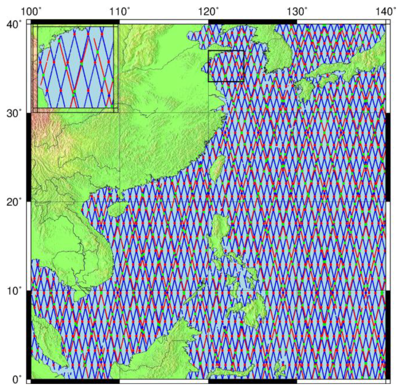
3.1. Multi-Mission Crossover Analysis

Measurements from radar altimetry missions are classically validated at regional to global scales using relative calibration approaches based on statistical analysis at crossover points intra- and intermissions. Honestly, the smaller difference for intramission situation indicates better stability and internal conforming accuracy for onboard instruments while those crossover discrepancies between multimissions are more reliable for evaluating the range precision between altimetry measurements. Accordingly, we planned to firstly assess the HY-2A performance by analyzing crossover discrepancies with another typical high-precision mission. Meanwhile, the crossover difference for intramission situation is also considered for evaluating inner coincidence.

The satellite mission SARAL/AltiKa (hereafter referred as SARAL), which was launched in March 2013 by the Centre National d’Etudes Spatiales (CNES) and the Indian Space Research Organization (ISRO), shows outstanding performance in providing high-precision measurements due to the following improvements. SARAL operates at Ka-band frequency (35.75 GHz) and has a relatively small pulse-limited footprint and beam width in contrast to traditional Ku-band altimeters, which should decrease the contamination from bright off-nadir reflection. Furthermore, the relatively large bandwidth of SARAL allows a better vertical range sampling (~31 cm) than for Ku-band radar altimeters (~47 cm) which should strongly improve the determination of range [21,22,23]. Consequently, the SARAL geophysical data record (GDR) from cycle 1 to 12 was used as calibration data in this study, which is a homogeneous data set corresponding to more than one year (14 March 2013 to 8 May 2014).

Returning to the theory of crossover methodology, the validity requires that SSH measurements be entirely corrected from all ocean variability between the intersected passes of altimeters, while these SSH variations are caused by ocean tide, solid earth tide, barometer tide and wind effects. Therefore, the relevant environmental and geophysical corrections of the altimeter range measurements have been applied to calculating SSH. These corrections include dry and wet tropospheric path delay, ionospheric correction, sea state bias, ocean tide, solid earth tide, pole tide, high frequencies wind effect, and inverted barometer correction. All these corrections are provided in GDR products for HY-2A and SARAL, respectively, and no extra updating procedure is applied in this study. The specific information is listed in

Table 3. List of parameters used to estimate the SSH for both HY-2A and SARAL missions.

Contrastive Parameters	HY-2A	SARAL
Cycle range	59–68	1–12
Time scope	2013.12.21–2014.5.10	2013.3.14–2014.5.8
Dry troposphere correction	ECMWF	ECMWF
Wet troposphere correction	Radiometer	Radiometer
Ionospheric correction	Dual-frequency	GIM
Sea state bias	NSOAS empirical solution	NOAA empirical solution
Ocean tide	GOT00.2	GOT4.8
Solid earth tide	Cartwright and Tayler tables	Cartwright and Tayler tables
Pole tide	Wahr [24]	Wahr [24]
Inverted barometer correction	ECMWF	ECMWF
High-frequency fluctuations	Mog2D model	Mog2D model
Mean sea surface	NSOAS gridding solution	MSS_CNES_CLS_2011

. Besides, the incompletely constrained time-varying effects of ocean surface will inevitably affect the crossover discrepancies for either intra- and intermissions. As a result, crossover differences with and without time limit need to be respectively considered during the statistical procedure. We selected the HY-2A data sets from E059 to E068 among the cross-mission validation based on the chosen SARAL data in order to ensure the overlap of measuring time.

Based on the procedures mentioned before, along-track SSH measurements are calculated for both HY-2A and SARAL missions. The HY-2A/HY-2A and SARAL/SARAL crossover points are respectively determined by fitting ground tracks of sample data, while the crossovers are defined as the positions where each satellite crosses its own ground position. In addition, the crossover points for intermissions are defined as the positions where HY-2A and SARAL cross the same sea surface position. To sum up, the geographical distributions of HY-2A data (red lines), SARAL data (blue lines), HY-2A/HY-2A (blue dots), SARAL/SARAL (red dots), and HY-2A/SARAL (green dots) crossovers are shown in Figure 3.

Following the calculated positions of crossover points, the minimum, maximum, mean, and root-mean-square (RMS) values of crossover discrepancies are computed between corresponding ascending and descending passes over ocean surfaces without and with time limits of 1, 2, 5 and 10 days, respectively. The specific results are listed in

Table 4. Statistical information of crossover differences under intramission situations. Unit: m.

Time Limit	HY-2A					SARAL
	Num	Min	Max	Mean	RMS	Num	Min	Max	Mean	RMS
--	5136	−0.995	0.998	0.083	0.232	32146	−0.976	0.893	0.016	0.142
≤10 days	816	−0.979	0.841	0.096	0.182	2937	−0.607	0.732	0.017	0.082
≤5 days	442	−0.931	0.841	0.090	0.177	1468	−0.255	0.297	0.016	0.071
≤2 days	242	−0.899	0.841	0.086	0.170	557	−0.232	0.279	0.014	0.062
≤1 day	143	−0.664	0.608	0.095	0.148	371	−0.196	0.279	0.015	0.061

, which indicate that the measurements within the shortest time limits have the best coincidence under each situation. The differences between GOT00 and GOT4.8 might be as large as a centimeter level and influential in comparing SSH between HY-2A and SARAL. Consequently, we use the GOT-e 4.7 model (http://web.cecs.pdx.edu/~zaron/pub/GOT-e.html), which contains GOT-compatible grids and provides more valid values to cover the shoreline, for updating corresponding ocean tide corrections for both missions. The intermission crossover analysis is thus executed twice and the statistical information is listed in

Table 5. Statistical information of crossover differences under intermission situation (‘HY’ and ‘SA’ represent HY-2A and SARAL, ‘OTC’ for ocean tide correction, while ‘_A’ and ‘_D’ denote ascending and descending passes, respectively). Unit: m.

Mission	Time Limit	OTC in GDR					Updated OTC with GOT-e
		Num	Min	Max	Mean	RMS	Num	Min	Max	Mean	RMS
HY_A & SA_D	--	13,784	−0.998	0.958	0.191	0.250	13,216	−0.999	0.980	0.070	0.199
	≤1 day	131	−0.804	0.543	0.242	0.140	127	−0.942	0.406	0.097	0.139
HY_D & SA_A	--	11,590	−0.999	0.917	0.100	0.206	11,302	−0.999	0.782	−0.029	0.190
	≤1 day	100	−0.868	0.641	0.092	0.151	99	−0.999	0.321	−0.046	0.155
HY_A & SA_A	--	418	−0.993	0.650	0.209	0.226	396	−0.993	0.515	0.081	0.181
	≤1 day	5	0.041	0.439	0.222	0.162	5	−0.097	0.312	0.087	0.165
HY_D & SA_D	--	359	−0.992	0.951	0.124	0.224	349	−0.717	0.802	−0.0002	0.201
	≤1 day	3	0.047	0.419	0.175	0.211	3	−0.078	0.294	0.046	0.210
HY & SA	--	26,151	−0.999	0.958	0.150	0.235	25,263	−0.999	0.980	0.024	0.201
	≤1 day	239	−0.868	0.641	0.178	0.184	234	−0.999	0.406	0.035	0.175

. HY-2A has a valid but slightly worse performance than SARAL according to crossover analysis for either intramission or intermission situations. Besides the close measuring time, the uniform GOT-e model also reduces the SSH discrepancies for intermissions. A preliminary conclusion is drawn that the accuracy of HY-2A measurements is around ~10 cm while the inherent uncertainty of SARAL is taken into account. This validation initially implies that HY-2A is capable of investigating marine gravity anomalies due to the new data coverage and reliable range precision.

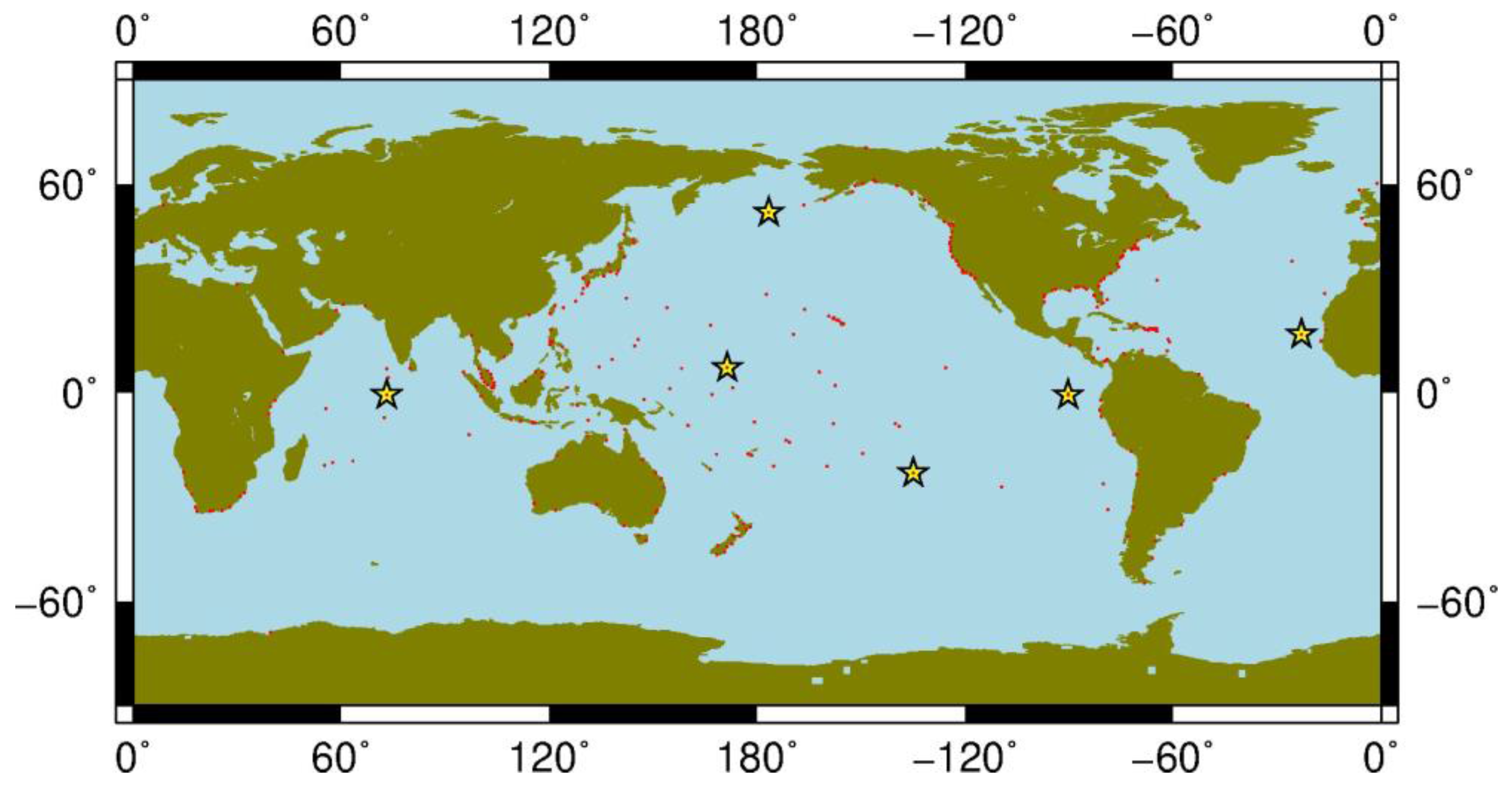
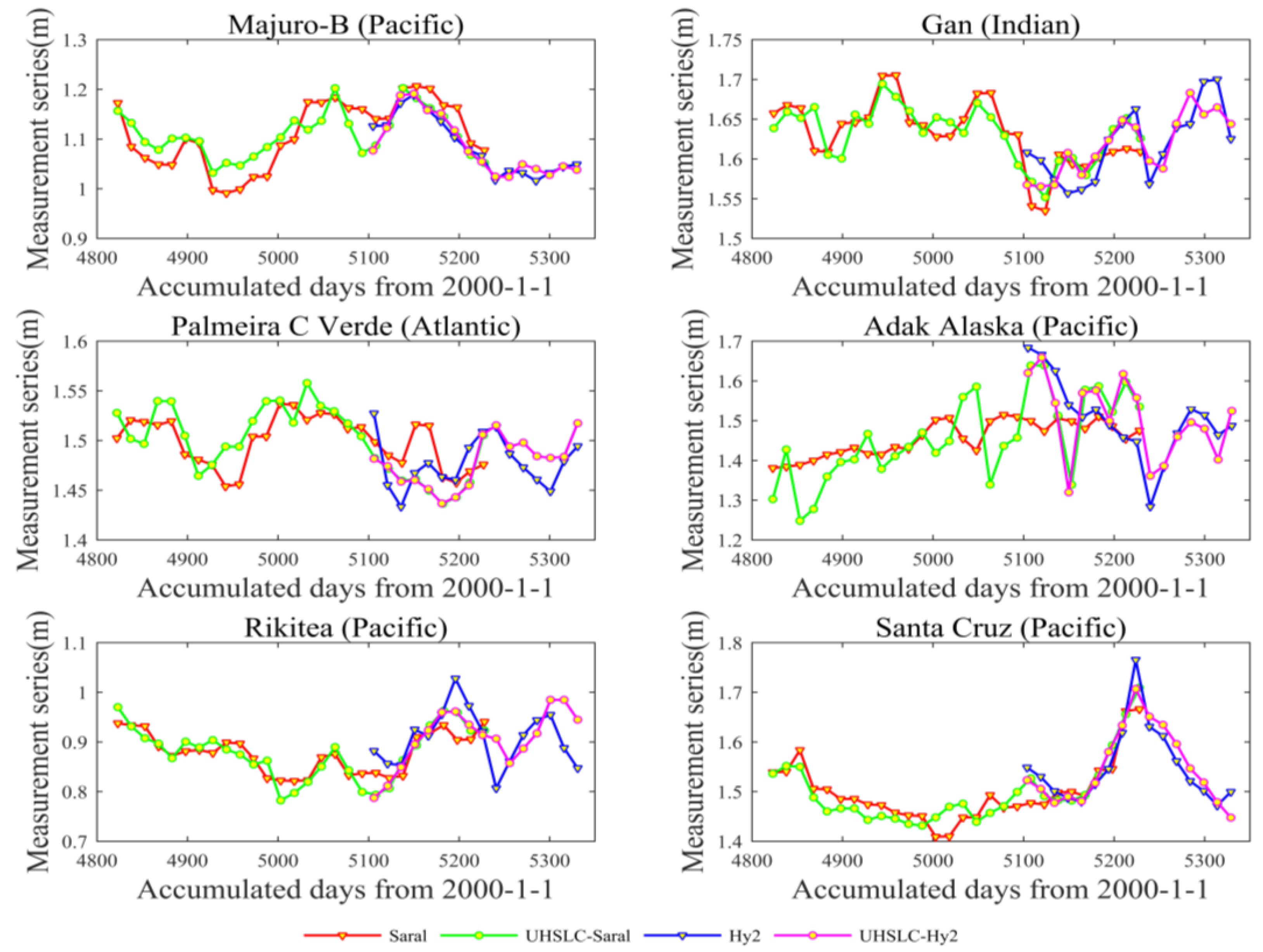
3.2. Validation with Tide Gauge Measurements

Besides the classical cross-mission validation, another well-known method is that sea surface heights from radar altimetry missions and in situ sea level measurements from tide gauges serve as each other’s buddy check. Consequently, we explored the performance of HY-2A observations in this section by comparing with time series of in situ sea level at tide gauge stations. Simultaneously, the 12 cycles of SARAL data were also evaluated during this procedure as a comparison. Nevertheless, the HY-2A time series were extended to 16 August 2014 (E075) because we wanted to involve the time series for as long as possible. This validation needed time overlap between altimetric measurements and in situ data series rather than between the two altimetric missions, while a significant data interruption happened to HY-2A after Cycle_E075.

Radar altimeters provide SSH observations, which need to be referenced and corrected from geophysical signals to provide sea level anomalies (SLA) compared with in situ measurements [25]. Therefore, the item of mean sea surface provided in level 2 products needs to be subtracted on the basis of calculating SSH as described in Section 3.1, after which along-track SLA series are obtained. We used valid-only satellite altimetry measurements relying on the quality flags and recommended data editing criteria in handbooks for both missions. The SLA series were then averaged onto a regular 1° × 1° grid, with a temporal resampling corresponding to data intervals at half a month [26].

The University of Hawaii Sea Level Center (UHSLC) offers tide gauge data with two levels of quality control (QC), where more rigorous QC requires more effort and a greater time lag. The Research Quality Data (RQD) sets received thorough QC and were considered to be the final science-ready data set, while the RQD were released 1–2 years after data was received from the data originators by UHSLC. Consequently, this RQD obtained via ftp://ftp.soest.hawaii.edu/uhslc/rqds was used for evaluating the performance of HY-2A measurements in this study. Although the spatial coverage of tide gauges is limited to coastal areas or isolated islands in the open ocean, the tide gauges will sample the ocean every hour, while at a given point, the satellite altimetry sampling is higher than ten days. The RQD is maintained by Pat Caldwell [27] and archived as the NOAA Joint Archive for Mean Sea Level (JAMSL) and only available from the UHSLC at hourly and daily resolution in order to avoid confusion with monthly data provided by the Permanent Service for Mean Sea Level (PSMSL). Consequently, the daily RQD was used for validation and a preprocessing procedure was applied to high-frequency in situ measurements for resampling a time series at the low frequency of altimetry data in 15-day intervals.

Based on the acquired global RQD sets and time span for two altimeter missions, 292 tide gauge stations (red dots in Figure 4) were probably for validation as only these in situ data series span across the period from 2013 to 2015, while 6 stations (yellow stars in Figure 4) among them were initially chosen for validation. All these 6 stations are located at the isolated islands over the open ocean and their geographical distributions represent the most situations over open oceans. The specific information for the chosen tide gauges is listed in

Table 6. Specific information of tide gauges in this study and corresponding correlation parameter (CI: Completeness index or percentage of data span without missing data; QC-YEARS: years which have received quality control).

Station	Latitude	Longitude	QC-YEARS	CI	Country	Contributor	Correlation Coefficient
							SARAL	HY-2A
Majuro-B	07°–07°N	171°–22°E	1993–2016	98	Rep. Marshall I.	Nat. Tidal Ctr., BOM	0.8079	0.9572
Gan	00°–41°S	073°–09°E	1987–2015	93	Rep. of Maldives	UH Sea Level Center	0.8224	0.7606
Palmeira C.Verde	16°–45°N	022°–59°W	2000–2015	92	Portugal	UH Sea Level Cente	0.6278	0.5135
Adak Alaska	51°–52°N	176°–38°W	1950–2016	92	USA	National Ocean Service	0.4677	0.6054
Rikitea	23°–08°S	134°–57°W	1969–2015	93	French Polynesia	UH Sea Level Center	0.8859	0.4982
Santa Cruz	00°–45°S	090°–19°W	1978–2015	96	Ecuador	UH Sea Level Center	0.9016	0.9281
Los Angeles, CA	33°–43°N	118°–16°W	1923–2016	99	USA	National Ocean Service	0.6589	0.6276
Cape May, NJ	38°–58°N	074°–58°W	1965–2016	91	USA	National Ocean Service	0.8171	0.7386
Ko Lak	11°–48°N	099°–49°E	1985–2017	95	Thailand	Naval Hydro. Dept.	0.9157	0.9407
Hong Kong-B	22°–18°N	114°–13°E	1986–2016	99	China	HK Observatory	0.8045	0.1467

.

After resampling the tide gauge time series, a set of correlation coefficients between the altimetry grids and the in situ records were computed. The maximum correlation is found at four 1° × 1° grid points and corresponding satellite altimetry time series are then extracted for plotting collation maps. The maps are shown in Figure 5 and corresponding correlation coefficients for altimetry and in situ series are listed in Table 6. The average values of correlation coefficients are respectively, 0.71 and 0.75 for HY-2A and SARAL. Both the missions provide valid performance due to our numerical test and the agreement is slightly better for in situ/SARAL than for in situ/HY-2A.

We also calculated the correlation coefficients for the tide gauge sites used for validation in the recent published studies [28,29]. Four UHSLC sites (Los Angeles, CA; Cape May, NJ; Ko Lak; Hong Kong) with required data series were selected due to the time-scope repetition with HY-2A and SARAL. The specific information for these sites is also listed in Table 6. Slightly larger average values of correlation coefficients are obtained for HY-2A (0.76) and SARAL (0.79), respectively, while the Hong Kong station is excluded for statistics due to the serious data loss which occurred at surrounding areas for HY-2A. We can draw a similar conclusion that the HY-2A altimeter provides valid sea surface height measurements but at a slightly lower accuracy level than SARAL. Although HY-2A provides noisier measurements than SARAL according to cross-mission analysis and verification with in situ tide gauge measurements, we also found the reliable side of HY-2A data and the explorer procedure about the two-pass waveform retracker for the purpose of gravity recovery is accordingly reasonable and necessary.

4. Two-Pass Retracker for HY-2A

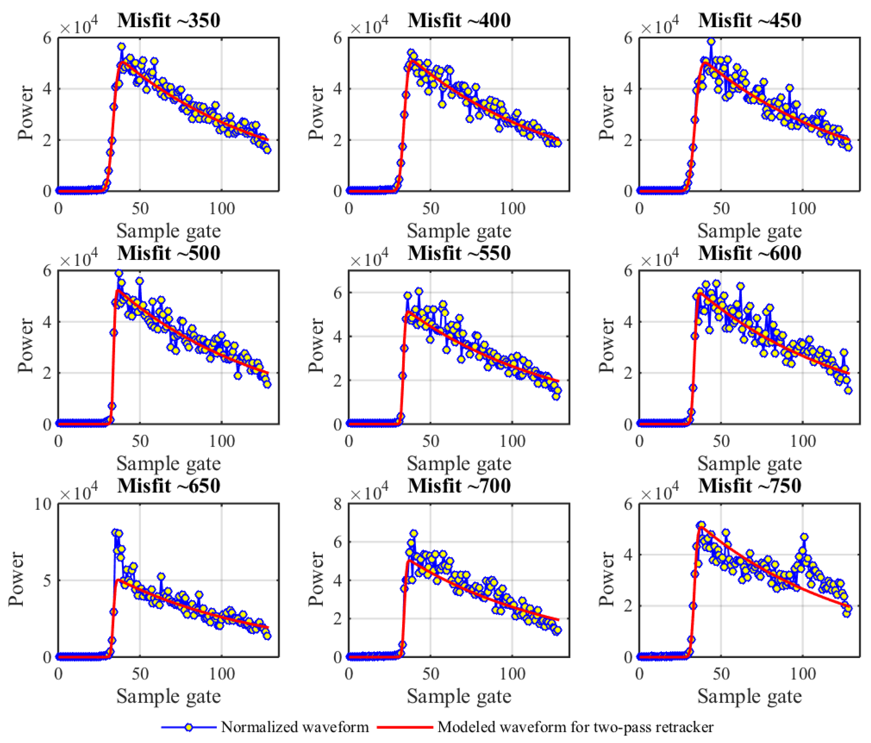
4.1. Theory of Two-Pass Retracker

Another major objective of our analysis is to evaluate whether the precision of HY-2A range measurements are further improved by using a two-pass waveform retracker which was proposed by Sandwell and Smith [9] initially and has already proven to be effective for other pulse-limited altimeter missions [19,20]. It is well known that waveform retracking is an effective and mature technique for solving limitations of data contamination by distribution of land or islands and diverse algorithms are developed either on empirical statistics or fitting functions for raw waveforms. Over the open ocean, the typical shapes of raw waveforms are well matched by the Brown [30] model with five parameters: arrival time, rise time, amplitude, square of the antenna mispointing angle, and thermal noise. The most concerning parameter for applications in marine gravity recovery is the arrival time, which provides an estimate of distance between the satellite and the instantaneous sea surface. In addition, the rise time and amplitude should also be set as variables for each raw waveform under any situations, while the thermal noise and square of the antenna mispointing angle can be treated as constant parameters for common waveforms obtained over open oceans.

Owing to the relationship between the errors in retracked estimates of arrival time and rise time [31], one effective approach to improving the precision of the arrival time is to fix the rise time parameter to a predetermined value based on surrounding waveforms. This can be accomplished with the two-pass retracking method where the waveforms are first fitted by the three-parameter Brown model (arrival time, rise time, and amplitude) with invariable constants describing thermal noise and antenna mispointing angles. The rise time parameter is then smoothed along-track, before retracking the waveforms a second time using a two-parameter Brown model (arrival time and amplitude) with the rise time being fixed to the along-track smoothed value [9]. Either the former three parameters or the latter two parameters will be solved during the weighted least squaring procedure, while the determination of the constants for describing thermal noise and antenna mispointing angles is critical before the two-pass model fitting procedure. The parameters and procedures involved in the two-pass retracker are deduced from the principle and power model of radar echoes over ocean surfaces.

The returned signal of conventional pulse-limited radar altimeters is proportional to the illuminated area scaled by the off-nadir roll-off of antenna gain pattern [30]. We are only interested in the slopes of SSH when using vertical deflection as an intermediate variable for recovering marine gravity field, and the constant offset with long-wave characteristics can be ignored accordingly. We also consider the case where the antenna bore sight is normally pointed to nadir. Under these simplifying assumptions, the power in the returned waveform can be modeled as following Equation (1), where A is the amplitude, t₀ is the arrival time, t is time for each sample gate, σ is the effective pulse length, and α is the trailing edge decay factor [32]. The effective pulse length σ can be calculated from two factors σ² = σ_h² + σ_p². The σ_h is the broadening of the pulse due to the interaction of ocean waves σ_h = SWH/2c, where c is the transferring speed of radar signals. The σ_p = 0.513τ_p is the standard deviation of the length of the outgoing pulse where τ_p = 1/B and B represents the chirp bandwidth for HY-2A (Ku: 320 MHz/80 MHz/20 MHz; C: 160 MHz). Three bandwidths for chirp signals are adopted in Model Compatible Tracker (MCT): the 320 MHz signal is arranged for oceanic measurement while 80 MHz is for the coastal zone, and the 20 MHz is for land or ice coverage. The trailing edge decay factor α mostly depends on the square of off-nadir pointing angle and can be treated as a constant value for HY-2A. Therefore, the fitting model has only three parameters [A, t₀, σ_h] to be solved by using the weighted least squares approach, while the constant value α should be predetermined.

$$M(t)=\frac{A}{2}[1+erf(\frac{t-t_0}{\sqrt{2\sigma }})]exp[-\alpha (t-t_0)]$$

(1)

$$X^2={\displaystyle \sum _{i=1}^N[\frac{P_i-M(t_i-t_0\cdot {\sigma }_h\cdot A)}{W_i}]}$$

(2)

$$W_i=\frac{P_i+P_0}{\sqrt{K}}$$

(3)

The chi-square measure of the misfit between the returned power samples P_i and the model estimate M(t_i) for the corresponding time t_i is formulated as Equation (2), where N is the number of gates (time samples) in the waveform, and W_i is the uncertainty assigned to each sample and given by Equation (3), where K is the number of statistically independent return echoes that were averaged to produce the waveform data records and P₀ is the power offset value reflecting the thermal noise level of the instrument. K = 96 is empirically determined for HY-2A as this mission collects ocean data at a pulse repetition frequency (PRF) of 1~4 kHz and similarly provides 20 Hz products in contrast to other altimeter missions [19]. P₀ will be given further discussion for selecting the optimal option in Section 4.2 although the results of the weighted least squares approach are largely insensitive to the numerical values for both K and P₀ [9].

In summary, the three parameters [A, t₀, σ_h] can be firstly calculated through an iterative weighted least squares approach once the numerical values of α and P₀ are given previously. Besides, a threshold retracker is also introduced to provide an initial estimate of t₀ to accelerate the iterative process, while the corresponding threshold value is defined with respect to the cumulative sum of waveform power and should be predetermined as well. Secondly, the rise time parameter about SWH is smoothed along-track using a low-pass filter having a 0.5 gain at a full wavelength of 90 km [9,19]. The final step of the two-pass retracker is to process the raw waveforms again by fixing the rise time parameter to the smoothed value and only solving for the parameters of arrival time and amplitude. Based on the theory and procedures of the two-pass retracker mentioned before, we will discuss how to determine the corresponding parameters in the next section.

4.2. Parameter Determination

The typical shapes of HY-2A waveforms over the open ocean are also well matched by the Brown model similar to other Ku-band missions. By contrast, both HY-2A and Jason-1 waveforms have equally spaced gates or samples although the counts are 128 and 104, respectively. Both sets of waveforms have a low noise power level prior to the sharp arrival of the main pulse, which starts to show up around gate 30~32. Besides, HY-2A waveforms have relatively steeper trailing edge decays and corresponding parameters describing waveform tail should be adjusted. The special deformed waveforms over sea ice-covered areas, large lakes, or land areas are not discussed in this paper as we focus on the performance of the two-pass retracker for optimal gravity field recovery over open ocean areas. Consequently, we initially assume that the two-pass retracker is still effective for this China altimetry mission and accordingly determine the adjusted parameters for fitting HY-2A echoes.

As discussed in the theory section, we began the analysis for the two-pass retracker with five unknown parameters [A, t₀, σ_h] and [α, P₀]. The first three parameters need to be calculated by using the weighted least squares approach, while the latter items should be predetermined once the objective waveform samples are sufficient. In addition, a threshold value needs to be predetermined for providing an initial estimate of t₀ to accelerate the iterative process. The determination of [α, P₀] and the threshold value was discussed on the basis of HY-2A waveform samples from Cycle_E115. Two descending passes labeled 222 and 260, respectively, were further selected for determining optimal parameters. Moreover, the screening criteria of valid results during the retracking procedure were also involved.

Firstly, α is a crucial parameter for fitting the waveforms, and the two-pass retracker is more sensitive to α than P₀ and threshold value [20]. The factor α depends mostly on the square of off-nadir pointing angle with a small order of magnitude and can be treated as a constant value for HY-2A. Based on the sampled passes, we gathered a number of successfully fitted waveform records and mean misfit values between original powers and modeled results respectively when using several typical values of α within the range of 0.005 and 0.015. Then we repeated this evaluation by sweeping through values of α at steps of 1.0 × 10⁻⁴ within range of 0.009 and 0.012. A best-fit α value of 0.0105 was approximately determined by considering both the valid records and misfit values for HY-2A. Meanwhile, the best-fit α values for different altimeter missions determined by previous studies are listed in

Table 7. The summarized best-fit α values for different satellite altimeter missions.

Mission	Geosat	ERS-1	Envisat	T/P Jason-1	CryoSat-2 LRM	CryoSat-2 SAR/SIN	SARAL	HY-2A
α value	0.006	0.022	0.09	0.0058	0.013	0.00744	0.0351	0.0105

for summarization [18,19,20].

Secondly, we investigated the relationship between waveform fitting results and the parameter P₀ describing the background noise level caused by temperature-dependent thermal noise in the receiver of the satellite altimeter. The magnitude of P₀ depends on the engineering characteristics of the altimeter and varies from the automatic gain control settings. Generally, P₀ can be either treated as a constant or empirically estimated through mean values or sum values of echo power for the first several sample gates [19,33]. 5 is used in this study for avoiding the false estimation due to complicated waveforms. Considering that the model-fitting results using the weighted least squares approach are largely insensitive to the numerical values of P₀, we treated P₀ as a constant similarly following the previous studies about ERS-1, Jason-1, and SARAL [19,20]. Besides, the power value for each gate is scaled by an arbitrary value of 3.3 × 10⁶ to convert the original integers to floating point numbers and this scale value is completely irrelevant to the two-pass retracking procedure. Fortunately, the inheritance numerical value of P₀ from Jason-1 (5500) is still reliable for HY-2A waveforms under the selected scale value (3.3 × 10⁶) because the ratios between the background noise level and the maximum power of echoes are similar for both missions.

Thirdly, a threshold value with respect to the cumulative sum of waveform power needs to be predetermined for providing an initial estimate of t₀ to accelerate the iterative process. Actually, the two-pass retracking results through iterative fitting are largely insensitive to the threshold value according to our experiments. Accordingly, we determined the optimal threshold value by minimizing the difference with respect to the results of the threshold retracker developed by Davis [34] for an exact initial objective gate, which leads to a valid threshold value of 0.015 for HY-2A.

Further discussion is needed about seriously deformed waveforms that will get unreliable results after the retracking procedure once the predetermined parameters [α, P₀] are given. Accordingly, we developed a waveform editing criteria based on estimated parameters [A, σ_h] as well as the fits to the waveforms executed. The editing threshold was established by constructing histograms of amplitude, chi-square misfit, and SWH versus standard deviation of the arrival time parameter. For HY-2A, valid waveforms should have model amplitudes within the range of 40,000–80,000, while the chi-squared misfit measurement should not exceed 800. The majority values of chi-squared misfit measurement are distributed within the range of 350~800 for valid retracked results. We also removed waveforms having SWH outside of the range 0.3–10 m for excluding observations over extremely unusual sea state conditions. Considering the robustness of the threshold retracker, we adopted the estimated results by the predetermined threshold instead when the HY-2A waveform records failed the editing criteria of the two-pass retracker.

While the predetermined parameters, threshold value, and waveform editing criteria were given, the results of the least squares fit of model waveforms and original waveform shapes are shown in Figure 6 for typical values of chi-squared misfit measurements. After examining thousands of waveforms over a range of sea states, we generally found that the fit to the HY-2A data is visually good, which suggested that the predetermined parameters were reliable. In accordance with the analysis by Garcia et al. [19], we also found a significant improvement (~5%) in the 20-Hz range precision if the least squares analysis was performed on three adjacent waveforms simultaneously, assigning the two outlier waveforms 1/2 the weight of the central waveform. Further enlargement of this three-waveform window did not reduce the range noise but increased processing time.

Once the two-pass retracker with three parameters [A, t₀, σ_h] to be solved in the first step was optimized for selected constant parameters [α, P₀] and threshold value, we retracked the complete Cycle_E115 with the full three-parameter model and corresponding waveform editing criteria. Then the rise time parameter was low-pass filtered with its 0.5 gain at a full wavelength of 90 km. The final step was to retrack the waveforms by fixing the rise time parameter to the smoothed value and only solving the parameter of the arrival time and amplitude.

5. Discussion

To assess the noise level of HY-2A data by the two-pass retracker, we performed a statistical analysis on the retracked SSH values (altitude minus range). All the corrections for path delay and geophysical environment were considered using items supplied by level 2 products. The noise was estimated as the standard deviation of the SSH with respect to the mean difference from the EIGEN6C4 model computed over a 1-second interval. The EIGEN6C4 model was used to account for areas of very steep geoid gradient where there could be a significant height variation (>20 mm) over the 7-km distance that the ground track moves in one second. This involved the provided 20 estimates corresponding to the HY-2A sampling rate along ground tracks.

Figure 7 shows the noise levels for the HY-2A sample pass labeled 260 in Cycle_E115. The noise level in the solved arrival time from the waveform leading edge should increase along with enhancing SWH and we plotted the noise level versus SWH thusly. Figure 7 also shows three independent estimates of noise level: the initial estimates derived from the retracked range measurement in SDR (red dots), the estimates from 3-parameter retracking (green dots), and ultimate 2-parameter retracking (blue dots), respectively. Additionally, the solid smoothed curves in the subgraph below with three corresponding colors are median averages of these estimates in 0.5-m SWH bins. The noise levels of three-parameter solutions and retracked results in SDR are at a similar level, while the latter is slightly superior. One more important finding is that the noise level of two-parameter retracked data is significantly lower than that for three-parameter solutions. Under the typical conditions of 2-m SWH, mean values of standard deviation for SDR, 3-parameter, and 2-parameter results are, respectively, 66.3, 67.1 and 40.9 mm for HY-2A, which is comparable to typical altimeter missions. The values for 3-parameter and 2-parameter retracked Jason-1 are, respectively, 75.9 and 46.4 mm, while CryoSat-2 LRM results are 64.7 and 42.7 mm [19]. This also demonstrates that the 2-parameter retracking decreases the noise level by a factor of 1.6 with respect to 3-parameter retracking, which is very close to the expected noise reduction of 1.57 based on the Monte Carlo simulation [9].

Spectral analysis is another effective way of analyzing the signal and noise ratio in the altimeter observations. On the basis of the Welch method [35], the power spectral density of along-track SSH for 3-parameter and 2-parameter retracked HY-2A data were respectively estimated using MATLAB and shown in Figure 8a. Both spectra show a rapid increase in power for wavelengths greater than 10 km and both the 3- and 2-parameter show a white noise level at wavelengths less than about 5 km. To highlight the differences between the two spectra, we calculated the spectra of the difference series between them as shown in Figure 8b. The increase in the difference spectra for wavelengths shorter than 90 km simply reflects the wavelength over which the SWH is smoothed between the two steps of iterative retracking procedures. At longer wavelengths, both the 3- and 2-parameter retrackers provide the same height measurement because the profiles contain the same SWH signal. The “hump” in the difference spectra between the wavelengths of 90 and ~5 km is also seen in spectra of two-pass retracked data from other pulse-limited altimeter missions [19,20]. This also demonstrates the band of wavelengths where two-pass retracking provides the most benefit [9].

The discrepancy at crossover points is another important index factor for assessing the accuracy of inner coincidence for altimeter SSH observations as mentioned before. Based on the HY-2A SDR data from Cycle_E115 over the southeastern China seas (100°~140°E, 0°~40°N), the statistic values of discrepancy at crossover points for three retracked results (SDR; 3-parameter and 2-parameter) are listed in

Table 8. Statistics of the SSH discrepancy at crossover points over southeastern China seas for HY-2A (Cycle_E115) and Jason-1 (Cycle500) sample data Unit: m.

Mission	Retracker Description	Crossover Points	Min	Max	MEAN	RMS
HY-2A	No retracker	125	−0.984	0.958	−0.287	0.412
	SDR—MLE4	125	−0.985	0.833	−0.280	0.391
	3-parameter	125	−0.975	0.916	−0.290	0.389
	2-parameter	125	−0.918	0.630	−0.272	0.377
Jason-1 GM	No retracker	126	−1.996	1.031	0.026	0.439
	SDR—MLE3	126	−0.713	0.547	0.048	0.191
	3-parameter	126	−0.531	1.286	0.072	0.230
	2-parameter	126	−0.446	1.006	0.066	0.208

, while the corrections for path delay and geophysical environment are also considered using items supplied by level 2 products. In addition, the corresponding results for Jason-1 GM data from Cycle500 are similarly calculated for comparison.

Table 8 indicates that all the three retracked results show improvement with respect to results without any retracker, and more remarkable for Jason-1. Moreover, the ultimate retracked results derived from the 2-parameter model are slightly superior to that of the 3-parameter model for both missions, which proves that the second iterative fitting procedure with smoothed SWH values as priority information does bring improvement for range precisions. In addition, the larger discrepancies may lead to an initial conclusion that the precision of HY-2A SSH is slightly lower than Jason-1 data, which is consistent with the previous conclusion in Section 3. Nevertheless, the accuracy improvement by the two-pass retracker was verified for both missions and fortunately HY-2A can potentially calculate sea surface slopes at a similar accuracy level with respect to Jason-1 GM data due to the statistics of standard deviation over a 1-second interval.

We also introduced the DW-TR retracker proposed by Huang et al. [28] for comparison based on the same sequence of HY-2A waveforms. The sample data (Cycle_E075 Pass_001) is located at the Gulf of Alaska and contains 535 waveforms with an offshore distance of less than ~200 km. The range corrections for the sample data with respect to corresponding offshore distances are plotted in Figure 9. The comparison shows that the correlation coefficient is large (0.92) for typical waveforms with offshore distance larger than 50 km, and it dramatically declines to ~0.10 for contaminated waveforms with offshore distances less than 50 km. The two-pass retracker pays more attention to optimal gravity recovery over the open ocean, while the DW-TR retracker focuses mostly on the coastal applications. As a result, we can initially draw the conclusion that the two-pass waveform retracker is valid over the open ocean.

Moreover, the 2nd-step of the two-pass retracker (red lines) got a closer result with DW-TR retracker than the 1st step. It’s hard to evaluate which retracker is more accurate relying on the current comparison. However, the accuracy improvement between the two steps of the retracker is detectable if we take the DW-TR result as reference. This improvement is also verified three other ways described before, STD calculation, power spectral density estimation, and crossover analysis. It’s reasonable to draw the conclusion that the two-pass retracker can bring range precision enhancement for HY-2A.

6. Conclusions

The validation activities represent an essential part of describing HY-2A altimetry data quality assessment and allow a quick feedback to operational teams and users in the altimetry community. Based on the investigations performed in this study, HY-2A firstly provides unique data coverage over ocean regions within 80°N and 80°S according to its specific orbital parameters with respect to other altimetric missions. Secondly, HY-2A provides reliable measurements in level 2 products based on the analysis of the multimission crossover discrepancies and the exterior verification with tide gauge measurement series. Thirdly, the two-pass retracker does bring improvement of HY-2A range precision and significant decline of noise level by a factor of 1.6, similar to previous pulse-limited altimeter missions.

In spite of the declined accuracy level of SSH observations with respect to SARAL based on our analysis, the along-track variances over a 1-second interval for retracked HY-2A results stay at a comparable level with respect to other missions (e.g., Jason-1/GM, CryoSat-2/LRM), which is an indicator for calculating reliable sea surface slopes. Additionally, the new data coverage due to HY2A’s individual orbital parameters may provide detective signals over somewhere unreached previously. Therefore, the accumulation of HY-2A data, especially for the GM phase recently, provides a great opportunity to explore the finer structure of marine gravity fields.

Almost 5 years ago, marine gravity fields having accuracies of 3~5 mGal (e.g., S&S V18 [18] and DNSC08 [11]) were based primarily on dense track coverage from 18 months of Geosat data from geodetic missions collected in the early 1990s and 12 months of European Remote-Sensing Satellite-1 (ERS-1/GM) data collected in 1995~1996. Over the last five years, the latest global mainstream marine gravity model such as DTU13 [36] and V23.1 [37] have got precision breakthrough at 1~3 mGal which mainly benefits from new missions with nonrepetitive ground tracks such as Jason-1/GM and CryoSat-2/369d. Moreover, both the orbits of SARAL and HY-2A satellites began to drift by up to 10 km from their initial 35-day track and 14-day track, respectively, and resulted in several cycles of altimeter data for new ocean coverage. Consequently, there are enough reasons to believe that the objective of 1-mGal accuracy and 1-minute resolution for the global marine gravity field is accessible in the recent future. Besides, the next big step in gravity field improvement may come with the higher range precision and finer resolution provided by the planned SWOT mission, which is scheduled for launch in 2020 [38].

References

1. Rapp, R.H. Geos 3 data processing for the recovery of geoid undulations and gravity anomalies. J. Geophys. Res. 1979, 84, 3784–3792. [Google Scholar] [CrossRef]
2. Haxby, W.F.; Karner, G.D.; Labrecque, J.L.; Weissel, J.K. Digital images of combined oceanic and continental data sets and their use in tectonic studies. EOS Trans. Am. Geophys. Union 1983, 64, 995–1004. [Google Scholar] [CrossRef]
3. Sandwell, D.T.; Smith, W.H.F. Marine gravity anomaly from Geosat and ERS1 satellite altimetry. J. Geophys. Res. 1997, 102, 10039–10054. [Google Scholar] [CrossRef]
4. Andersen, O.B.; Knudsen, P. Global marine gravity field from the ERS-1 and Geosat geodetic mission altimetry. J. Geophys. Res. 1998, 103, 8129–8137. [Google Scholar] [CrossRef]
5. Hwang, C. Inverse Vening Meinesz formula and deflection-geoid formula: Applications to the predictions of gravity and geoid over the South China Sea. J. Geodesy 1998, 72, 304–312. [Google Scholar] [CrossRef]
6. Sandwell, D.T.; Garcia, E.S.; Soofi, K.; Wessel, P.; Chandler, M.; Smith, W.H. Towards 1-mGal accuracy in global marine gravity from Cryosat-2, Envisat and Jason-1. Lead. Edge 2013, 32, 892–898. [Google Scholar] [CrossRef]
7. Andersen, O.B.; Jain, M.; Knudsen, P. The Impact of Using Jason-1 and Cryosat-2 Geodetic Mission Altimetry for Gravity Field Modeling. IAG 150 Years Symp. 2016, 143, 205–210. [Google Scholar]
8. Zhang, S.; Sandwell, D.T.; Jin, T.; Li, D. Inversion of marine gravity anomalies over southeastern China seas from multi-satellite altimeter vertical deflections. J. Appl. Geophys. 2017, 137, 128–137. [Google Scholar] [CrossRef]
9. Sandwell, D.T.; Smith, W.H.F. Retracking ERS-1 altimeter waveforms for optimal gravity field recovery. Geophys. J. Int. 2005, 163, 79–89. [Google Scholar] [CrossRef]
10. Hwang, C.; Guo, J.; Deng, X.; Hsu, H.Y.; Liu, Y. Coastal gravity anomalies from retracked Geosat GM altimetry: Improvement, limitation and the role of airborne gravity data. J. Geodesy 2006, 80, 204–216. [Google Scholar] [CrossRef]
11. Andersen, O.B.; Knudsen, P.; Berry, P. The DNSC08GRA global marine gravity field from double retracked satellite altimetry. J. Geodesy 2010, 84, 191–199. [Google Scholar] [CrossRef]
12. Sandwell, D.T. Antarctic marine gravity field from high-density satellite altimetry. Geophys. J. Int. 1992, 109, 437–448. [Google Scholar] [CrossRef]
13. Zhao, G.; Zhou, X. Precise orbit determination of Haiyang-2 using satellite laser ranging. Chin. Sci. Bull. 2013, 58, 589–597. [Google Scholar] [CrossRef]
14. Legeais, J.-F.; Ablain, M.; Faugère, Y.; Mertz, F.; Soussi, B.; Vincent, P. HY-2A and DUACS (Data Unification and Altimeter Combination System) altimeter products. In Proceedings of the OSTST 2012 (Ocean Surface Topography Science Team) Meeting, Venice, Italy, 22–29 September 2012. [Google Scholar]
15. Bao, L.; Gao, P.; Peng, H.; Jia, Y.; Shum, C.K.; Lin, M.; Guo, Q. First accuracy assessment of the HY-2A altimeter sea surface height observations: Cross-calibration results. Adv. Space Res. 2015, 55, 90–105. [Google Scholar] [CrossRef]
16. Peng, H.; Lin, M.; Mu, B. Global statistical evaluation and performance analysis of HY-2A satellite radar altimeter data. Haiyang Xuebao 2015, 37, 54–66. (In Chinese) [Google Scholar]
17. Yang, L.; Zhou, X.; Lin, M.; Lei, N.; Mu, B.; Zhu, L. Global statistical assessment of HY-2A altimeter IGDR data. Prog. Geophys. 2016, 31, 629–636. (In Chinese) [Google Scholar] [CrossRef]
18. Sandwell, D.T.; Smith, W.H.F. Global marine gravity from retracked Geosat and ERS-1 altimetry: Ridge segmentation versus spreading rate. J. Geophys. Res. 2009, 114, B014411. [Google Scholar] [CrossRef]
19. Garcia, E.S.; Sandwell, D.T.; Smith, W.H.F. Retracking CryoSat-2, Envisat, and Jason-1 radar altimetry waveforms for improved gravity field recovery. Geophys. J. Int. 2014, 196, 1402–1422. [Google Scholar] [CrossRef]
20. Zhang, S.; Sandwell, D.T. Retracking of SARAL/AltiKa Radar Altimetry Waveforms for Optimal Gravity Field Recovery. Mar. Geodesy 2017, 40, 40–56. [Google Scholar] [CrossRef]
21. Prandi, P.S.; Philipps, S.; Pignot, V.; Picot, N. SARAL/AltiKa global statistical assessment and cross-calibration with Jason-2. Mar. Geodesy 2015, 38, 297–312. [Google Scholar] [CrossRef]
22. Vu, P.; Frappart, F.; Darrozes, L. Multi-Satellite Altimeter Validation along the French Atlantic Coast in the Southern Bay of Biscay from ERS-2 to SARAL. Remote Sens. 2018, 10, 93. [Google Scholar] [CrossRef]
23. Salameh, E.; Frappart, F.; Marieu, V. Monitoring Sea Level and Topography of Coastal Lagoons Using Satellite Radar Altimetry: The Example of the Arcachon Bay in the Bay of Biscay. Remote Sens. 2018, 10, 297. [Google Scholar] [CrossRef]
24. Wahr, L.W. Deformation of the earth induced by polar motion. J. Geophys. Res. (Solid Earth) 1985, 90, 9363–9368. [Google Scholar] [CrossRef]
25. Valladeau, G.; Legeais, J.F.; Ablain, M.; Guinehut, S.; Picot, N. Comparing altimetry with tide gauges and Argo profiling floats for data quality assessment and mean sea level studies. Mar. Geodesy 2012, 35, 42–60. [Google Scholar] [CrossRef]
26. CalVal In-Situ Altimetry/tide Gauges. Validation of Altimeter Data by Comparison with Tide Gauge Measurements; CLS: Ramonville St-Agne, France, 2014; CLS.DOS/NT/13-285, Issue 1.1, Nomenclature: SALP-RP-MA-EA-22294-CLS. [Google Scholar]
27. Caldwell, P.C.; Merrifield, M.A.; Thompson, P.R. Sea Level Measured by Tide Gauges from Global Oceans—The Joint Archive for Sea Level Holdings (NCEI Accession 0019568); Version 5.5; NOAA National Centers for Environmental Information: Silver Spring, MD, USA, 2015.
28. Huang, Z.; Wang, H.; Luo, Z.; Shum, C.K.; Tseng, K.-H.; Zhong, B. Improving Jason-2 Sea Surface Heights within 10 km Offshore by Retracking Decontaminated Waveforms. Remote Sens. 2017, 9, 1077. [Google Scholar] [CrossRef]
29. Xu, X.; Birol, F.; Cazenave, A. Evaluation of Coastal Sea Level Offshore Hong Kong from Jason-2 Altimetry. Remote Sens. 2018, 10, 282. [Google Scholar] [CrossRef]
30. Brown, G. The average impulse response of a rough surface and its applications. IEEE Trans. Antennas Propag. 1977, 25, 67–74. [Google Scholar] [CrossRef]
31. Maus, S.; Green, C.M.; Fairhead, J.D. Improved ocean-geoid resolution from retracked ERS-1 satellite altimeter waveforms. Geophys. J. Int. 1998, 134, 243–253. [Google Scholar] [CrossRef]
32. Rodriguez, E. Altimetry for non-Gaussian oceans: Height biases and estimation of parameters. J. Geophys. Res. Oceans 1988, 93, 14107–14120. [Google Scholar] [CrossRef]
33. Martin, T.V.; Zwally, H.J.; Brenner, A.C.; Bindschadler, R.A. Analysis and retracking of continental ice sheet radar altimeter waveforms. J. Geophys Res. 1983, 88, 1608–1616. [Google Scholar] [CrossRef]
34. Davis, C.H. A surface and volume scattering retracking algorithm for ice sheet satellite altimetry. IEEE Trans. Geosci. Remote Sens. 1993, 31, 811–818. [Google Scholar] [CrossRef]
35. Welch, P.D. The use of fast Fourier transforms for the estimation of power spectra: A method based on time averaging over short, modified periodograms. IEEE Trans. Audio Electroacoust. 1967, 15, 70–73. [Google Scholar] [CrossRef]
36. Andersen, O.B.; Knudsen, P.; Kenyon, S.; Holmes, S. Global and arctic marine gravity field from recent satellite altimetry (DTU13). In Proceedings of the 76th EAGE Conference and Exhibition, Amsterdam, The Netherlands, 16–19 June 2014. [Google Scholar]
37. Sandwell, D.T.; Müller, R.D.; Smith, W.H.F.; Garcia, E.; Francis, R. New global marine gravity model from CryoSat-2 and Jason-1 reveals buried tectonic structure. Science 2014, 346, 65–67. [Google Scholar] [CrossRef] [PubMed]
38. Fu, L.L.; Ubelmann, C. On the transition from profile altimeter to swath altimeter for observing global ocean surface topography. J. Atmos. Ocean. Technol. 2013, 31, 560–568. [Google Scholar] [CrossRef]
Figure 1. Distribution of multisatellite altimetry data over Research Region (HY-2A/ERM: red; Jason-1/ERM: yellow; Jason-1 Tandem/ERM: orange; Geosat/ERM: purple; Envisat/35 days: blue; Envisat/30 days: green; CryoSat-2/369 days: olive).
Remotesensing 10 00507 g001
Figure 2. Distribution of HY-2A data over locally magnified region and research area (ERM: red; GM: yellow).
Remotesensing 10 00507 g002
Figure 3. Distribution of HY-2A and SARAL altimetry data and corresponding crossover points intra- and intermissions (Red line: HY-2A data; Blue line: SARAL data; Blue dots: crossover points for HY-2A itself; Red dots: crossover points for SARAL itself; Green dots: crossover points for HY-2A and SARAL intermissions).
Remotesensing 10 00507 g003
Figure 4. The 6 tide gauge stations (yellow stars) considered in this study. Red dots denote 292 tide gauge stations that span across the period from 2013 to 2015.
Remotesensing 10 00507 g004
Figure 5. Comparison of HY-2A and SARAL SLA series with tide gauge sea level series at 6 stations (Red: SARAL; Green: TG for SARAL; Blue: HY-2A; Purple: TG for HY-2A).
Remotesensing 10 00507 g005
Figure 6. Least squares fit of model waveform of HY-2A for predetermined parameters (Blue: normalized waveform in SDR; Red: Modeled waveform of two-pass retracker).
Remotesensing 10 00507 g006
Figure 7. Standard deviation of retracked height with respect to EIGEN6C4 for HY-2A (Red—sensor data record; Green—3-parameter retracking; Blue—2-parameter retracking).
Remotesensing 10 00507 g007
Figure 8. (a) Power spectral density of along-track retracked height from 3-parameter (blue) and 2-parameter (red) model for HY-2A data; (b) Power spectral density of along-track retracked height difference between 3-parameter and 2-parameter model for HY-2A. Wavelength range of spectral hump within 5–90 km is marked by vertical dashed lines.
Remotesensing 10 00507 g008
Figure 9. Comparison of range correction series for two-pass retracker and DW-TR retracker (Green: Two-pass retracker 1st step; Red: Two-pass retracker, 2nd step; Blue: DW-TR results).
Remotesensing 10 00507 g009