Estimation of Global Vegetation Productivity from Global LAnd Surface Satellite Data

Abstract

Accurately estimating vegetation productivity is important in research on terrestrial ecosystems, carbon cycles and climate change. Eight-day gross primary production (GPP) and annual net primary production (NPP) are contained in MODerate Resolution Imaging Spectroradiometer (MODIS) products (MOD17), which are considered the first operational datasets for monitoring global vegetation productivity. However, the cloud-contaminated MODIS leaf area index (LAI) and Fraction of Photosynthetically Active Radiation (FPAR) retrievals may introduce some considerable errors to MODIS GPP and NPP products. In this paper, global eight-day GPP and eight-day NPP were first estimated based on Global LAnd Surface Satellite (GLASS) LAI and FPAR products. Then, GPP and NPP estimates were validated by FLUXNET GPP data and BigFoot NPP data and were compared with MODIS GPP and NPP products. Compared with MODIS GPP, a time series showed that estimated GLASS GPP in our study was more temporally continuous and spatially complete with smoother trajectories. Validated with FLUXNET GPP and BigFoot NPP, we demonstrated that estimated GLASS GPP and NPP achieved higher precision for most vegetation types.

1. Introduction

As vegetation productivity is one of the most variable components of the terrestrial carbon cycle, accurately estimating this component is important in research on terrestrial ecosystems, carbon cycles and climate change [1]. On a global scale, MOD17 products are the first operational data sets to regularly monitor global vegetation productivity from MODerate Resolution Imaging Spectroradiometer (MODIS). Eight-day gross primary production (GPP) and annual net primary production (NPP) with 1 km spatial resolution are components of the MOD17 product. MOD17 is derived from a light use efficiency (LUE) model [2,3] based on the MOD12 land cover product, Data Assimilation Office meteorological datasets, and the MOD15 Leaf Area Index (LAI) and Fraction of Photosynthetically Active Radiation (FPAR) products. Consequently, the uncertainties of these input data will influence the accuracy of the MOD17 product [1]. Therefore, estimating global vegetation productivity products from datasets with a higher precision is imperative for improving the quality of vegetation productivity products.

Studies have shown that the contaminated or missing MOD15 LAI and FPAR products may introduce some considerable errors to MODIS GPP and NPP products [4]. In addition, MOD15 LAI and FPAR products generated from individual satellite data have been demonstrated to be spatially and temporally discontinuous on regional and global scales, and are less representative in some vegetation types [5,6,7,8]. Thus, to generate more accurate and consistent GPP and NPP products, more consistent and higher quality LAI and FPAR datasets should be used. Global LAnd Surface Satellite (GLASS) LAI products were developed based on time-series MODIS and Advanced Very High Resolution Radiometer reflectance data using General Regression Neural Networks (GRNNs) trained with fused time-series LAI from MODIS and Carbon CYcle and Change in Land Observational Products from an Ensemble of Satellites (CYCLOPES) [9,10,11]. Studies [9,10,12] have shown that the GLASS LAI product achieves a higher precision than MODIS LAI and is more temporally continuous and spatially complete with smoother trajectories. Moreover, Xiao et al. [13] developed the GLASS FPAR product with continuous trajectories and high accuracy based on the GLASS LAI product. Therefore, more continuous results with higher precision may be obtained when estimating global vegetation productivity using GLASS LAI and FPAR products.

For the estimation of vegetation productivity, many models have been developed on both regional and global scales. Climate productivity models, such as the Miami model, Thornthwaite Memorial model [14], and Chikugo model [15], are based on the relationships between GPP/NPP and climate factors. LUE models have great potential to address the spatial and temporal dynamics of GPP/NPP [16], such as the Carnegie, Ames, Stanford Approach (CASA) [17] and the GLObal Production Efficiency Model (GLO-PEM) [18]. The basis of eco-physiological process models is ecological and biophysical process theories, such as the CENTURY [19], Terrestrial Ecosystem Model (TEM) [20], and Biome Bio-Geochemical Cycle (Biome-BGC) model [21]. MOD17 daily GPP and annual NPP products are derived from the LUE model. FPAR is related to GPP assimilation, and LAI is related to respiration when estimating NPP. However, daily MODIS Net Photosynthesis (PSNnet) does not include the calculation of growth respiration and maintenance respiration associated with living wood when compared with NPP. In this case, developing a more reliable algorithm to estimate global daily GPP and NPP by integrating high quality GLASS data and eco-physiological processes is of great significance.

The aims of this paper are (i) to generate more accurate and continuous global GPP and NPP products with GLASS data; (ii) to validate the GPP and NPP estimates, and to compare the results with products; and (iii) to analyze the temporal and spatial variation of global GPP and NPP from 2004 to 2012.

2. Materials and Methods

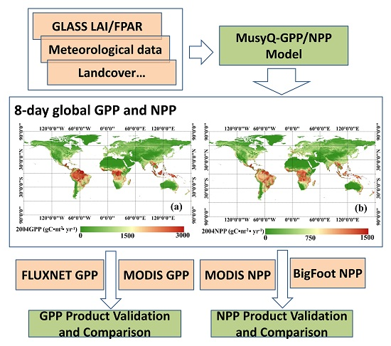
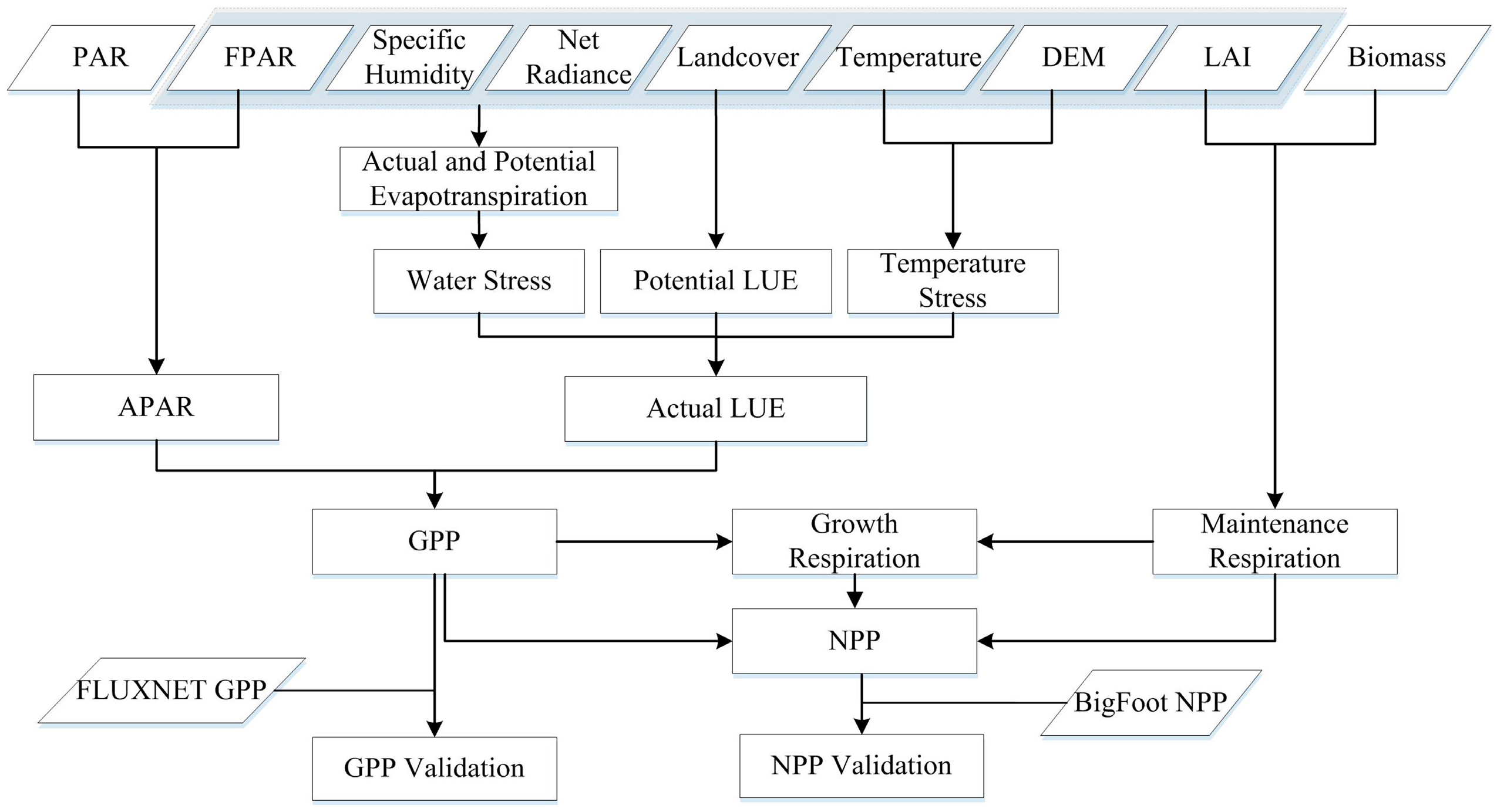
2.1. Method

2.1.1. Estimation of GPP and NPP

A flowchart of GPP and NPP estimation and validation is shown in Figure 1. To estimate global daily GPP/NPP by integrating remote sensing data and eco-physiological processes, the Multi-source data Synergized Quantitative (MuSyQ) NPP algorithm [22] was adopted in this paper. The MuSyQ-NPP algorithm is essentially a LUE model; thus, daily GPP could be described as:

GPP = ε × FPAR × PAR

(1)

where ε is the LUE, and PAR is the photosynthetically active radiation (PAR), which could be obtained from Global Land Data Assimilation System (GLDAS) incident shortwave radiation R using the following equation:

PAR = 0.5 × R

(2)

LUE may be influenced by many environmental stressors, such as low temperature and water shortage. In this condition, ε could be described as:

$$\epsilon ={\epsilon }_{max}\times f_1\left(T\right)\times f_2\left(\beta \right)$$

(3)

where ${\epsilon }_{max}$ is the biome-specific potential of LUE, and $f_1\left(T\right)$ and $f_2\left(\beta \right)$ are the down-regulation effects of temperature and water conditions on ${\epsilon }_{max}$, respectively. A biome-specific potential ${\epsilon }_{max}$ Look-Up Table (LUT) was established by referring to land cover categories according to the Biome Properties Look-Up Table (BPLUT) of the MODIS GPP/NPP algorithm [23]. It is noted that a potential ${\epsilon }_{max}$ value of 1.5 g C MJ⁻¹ for crops was used in the algorithm. $f_1\left(T\right)$ was calculated according to the CASA model [17]. The effect of water conditions on plant photosynthesis $f_2\left(\beta \right)$ could be described as:

$$f_2\left(\beta \right)=0.5+0.5ET/E{T}_P$$

(4)

where ET represents actual evapotranspiration, which is estimated from a modified P-M approach, LAI and Fcover products [22,24,25]. $E{T}_P$ represents potential evapotranspiration, which is estimated using the Priestley and Taylor (PT) equation [26].

NPP is the net flow of carbon from the atmosphere to plants, which is defined as the balance between GPP and autotrophic respiration.

$$NPP=GPP-R_a$$

(5)

where $R_a$ is autotrophic respiration. Autotrophic respiration (R_a) could be separated into two parts: maintenance respiration $R_m$, which refers to the energy necessary to maintain biomass, and growth respiration $R_g$ which refers to the energy needed for converting assimilates into new structural plant constituents.

$$R_a=R_m+R_g$$

(6)

When estimating $R_m$, non-forest and forest lands were estimated separately. For non-forest land, $R_m$ was estimated with LAI and specific leaf area (SLA).

$$R_m=LAI/SLA\times 0.5\times 2^{\left(T-T_b\right)/10}$$

(7)

where SLA was obtained from the BPLUT of MODIS GPP/NPP algorithm [23] in our model.

For forest land, $R_m$ was obtained by summing the maintenance respiration of leaves, stems, and roots [22].

$$R_{m,i}=M_i{r}_{m,i}{Q}_{10,i}^{T-T_b/10}$$

(8)

where $M_i$ is the biomass of plant component i, $r_{m,i}$ is maintenance respiration coefficient for component i, $Q_{10,i}$ is the temperature sensitivity factor, T is the daily average temperature and $T_b$ is the base temperature, $r_{m,i}$ is the maintenance respiration coefficient. Forest lands are classified into four classes: needle-leaf forests, broadleaved forests, mixed forests and others, and $Q_{10,i}$ and $r_{m,i}$ for each class are obtained according to the BPLUT of MODIS GPP/NPP algorithm [23]. Specifically, leaf mass is estimated from LAI and SLA:

$$M_1=LAI/SLA$$

(9)

Stem and root mass are obtained using:

$$M_2=biomass/\left(1+y\right)$$

(10)

$$M_3=y\times M_2$$

(11)

where y is the ecophysiological biome-specific constant obtained from the Boreal Ecosystem Productivity Simulator (BEPS) model [27]. The leaf, stem, fine root and coarse root respiration items were calculated separately, according to the BEPS model.

Growth respiration ($R_g$) was considered to be proportional to the difference between GPP and maintenance respiration ($R_m$):

$$R_g=\gamma \left(GPP-R_m\right)$$

(12)

where γ is the growth respiration coefficient and is defined as 0.25.

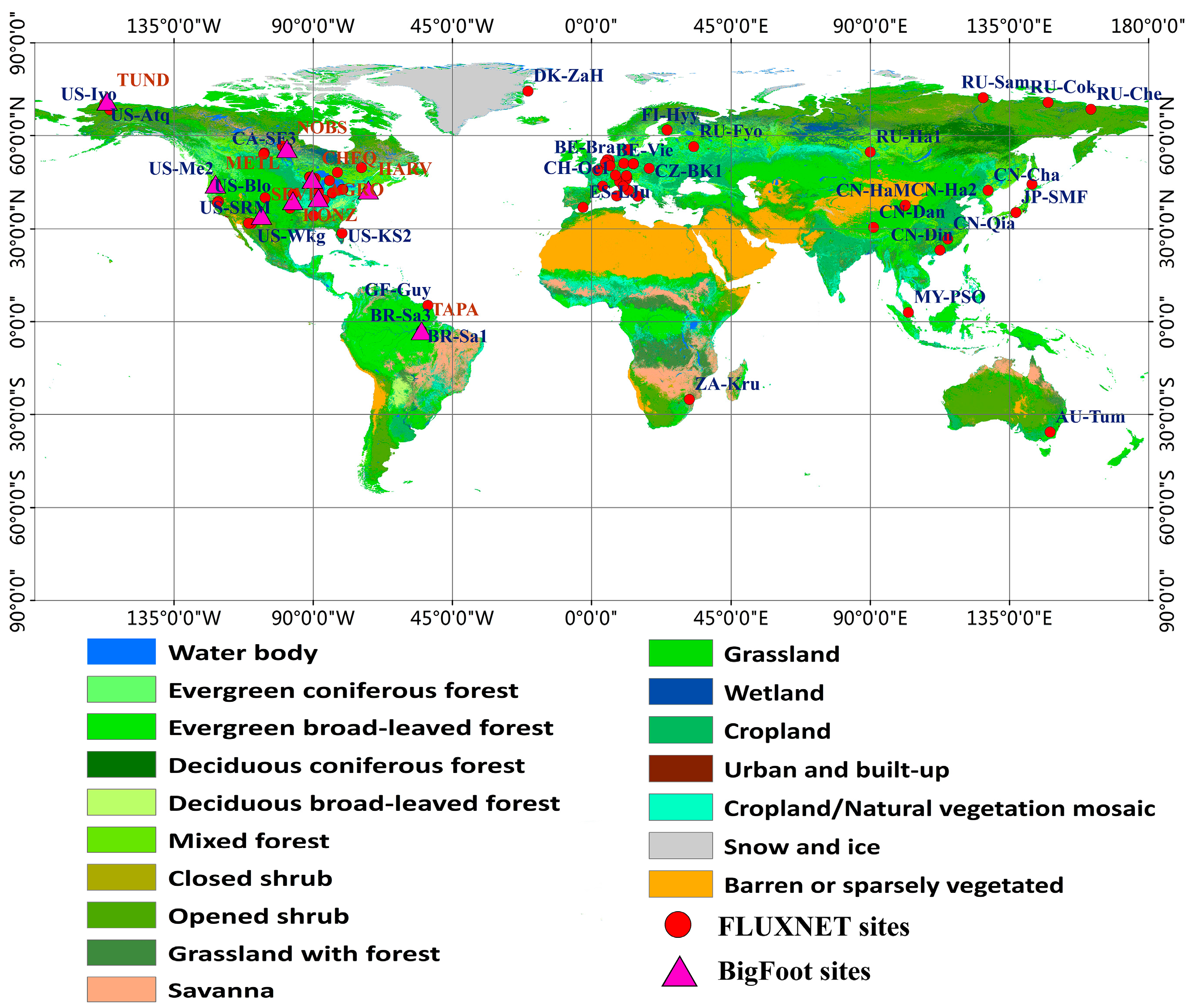
2.1.2. Validation of Estimated GLASS GPP and NPP

To assess the performance of the MuSyQ-NPP algorithm, FLUXNET GPP and BigFoot NPP were used to validate the GLASS GPP and NPP estimates. Specifically, eight-day GLASS GPP estimates were compared with ground level eight-day FLUXNET GPP, and the average GLASS NPP estimates in 2004, 2008 and 2012 at each Bigfoot site were compared with ground level yearly BigFoot NPP for 2000–2004.

2.2. Data and Data Processing

2.2.1. Remote Sensing Data

GLASS LAI/FPAR Products: The GLASS LAI/FPAR products, with a temporal resolution of eight days and a spatial resolution of 1 km, were generated and released by the Center for Global Change Data Processing and Analysis of Beijing Normal University [28]. They are also available from the Global Land Cover Facility [29]. The GLASS LAI product was estimated from time-series MODIS and AVHRR reflectance data using GRNNs, which were trained for each biome type by fusing MODIS and CYCLOPES LAI. The GLASS LAI product is believed to be more temporally continuous and spatially complete compared to the MODIS LAI product [11]. The GLASS FPAR product was generated from the GLASS LAI product; thus, it shows the same properties as the GLASS LAI product. Validation against the VAlidation of Land European Remote sensing Instrument (VALERI) ground-based estimates has shown that both GLASS LAI and FPAR products had high accuracy (RMSE = 0.7848 and R² = 0.8095 for the LAI product, RMSE = 0.1276 and R² = 0.8048 for the FPAR product) [10,13].

MODIS land cover product: The MODIS Land Cover Dynamics product (MCD12Q2) provided estimates of yearly vegetation phenology on a global scale [30]. The product identified 17 land cover classes defined by the International Geosphere Biosphere Program (IGBP) with a spatial resolution of 1 km, which includes 11 natural vegetation classes, three developed and mosaicked land classes, and three non-vegetated land classes [31].

TRAGL fractional vegetation cover (FCover) product: The TRAGL FCover product, with a temporal resolution of eight days and a spatial resolution of 1 km, was derived from the GLASS LAI product based on the method proposed by Xiao et al. [32]. The product is believed to be more spatially and temporally complete with continuous trajectories compared with the GEOV1 product. Direct validation with ground-based FCover estimates demonstrated that the TRAGL FCover product was generated with high accuracy (RMSE = 0.0865 and R² = 0.8848) [26].

Global Biomass Map: A global biomass map with a spatial resolution of 1 km was generated by the Carbon Dioxide Information Analysis Center (CDIAC) [33] using International Panel on Climate Change (IPCC) methods [34,35]. The global biomass carbon stocks were firstly estimated using the globally consistent default values provided for aboveground biomass [35], then belowground biomass (root) was added using the IPCC root to shoot ratios for each vegetation type.

2.2.2. Meteorological Data

Meteorological data were derived from Global Land Data Assimilation System (GLDAS) products [36]. GLDAS products were generated using four land surface models and data assimilation techniques with both satellite data and ground based observational data [37,38]. Daily near surface air temperature, near surface specific humidity, and net shortwave radiation were obtained in our study by averaging the GLDAS three-hour products. As the spatial resolution of this product was 0.25°, bilinear interpolation was adopted to generate the 1 km meteorological datasets.

2.2.3. Field Data

FLUXNET GPP data: FLUXNET is a global network of micrometeorological tower sites used to measure the exchanges of carbon dioxide, water vapor, and energy between the biosphere and atmosphere. This global network includes more than eight hundred active and historic flux sites, which are dispersed across most of the world’s climate space and across representative biomes. FLUXNET data are most commonly used in validation and calibration of ecosystem models, parameter estimation and optimization procedures in data assimilation systems [39,40]. In our study, daily GPP derived by the daytime partitioning method from 59 FLUXNET sites (See Table S1 in Supplementary Materials) was firstly collected, and then eight-Day GPP were obtained by averaging the daily GPP to validate our GPP estimates and MODIS GPP product [41]. Vegetation types in these FLUXNET sites include deciduous broadleaved forest (DBF), evergreen broadleaved forest (EBF), evergreen needle-leaf forest (ENF), cropland (CRO), grassland (GRA), and mixed forest (MF). The locations of FLUXNET sites used in this study, and the IGBP landcover classes are shown in Figure 2.

BigFoot NPP data: The overall objective of BigFoot was to provide ground validation for MODIS land cover, LAI, FPAR and NPP products [42]. Nine BigFoot sites were established from Alaska to Brazil. The BigFoot NPP product was generated using the Biome-BGC model [21], based on Landsat ETM+ derived land cover and LAI, tower measured meteorological data and eco-physical parameters. Each BigFoot NPP product covered a 7 × 7 km area with a temporal resolution of one year and a spatial resolution of 25 m. In our study, BigFoot NPP data were used to validate NPP estimates and the MODIS NPP product. Basic information on BigFoot sites is summarized in

Table 1. Basic information of BigFoot sites.

Site Name	Latitude	Longitude	Biome Type	Year
NOBS	55.8853	−98.4773	Boreal forest	2001–2003
AGRO	40.0067	−88.2915	Crop	2000
HARV	42.5285	−72.1729	Temperate mixed forest	2003
CHEQ	45.9453	−90.2731	Temperate mixed forest	2000–2002
METL	44.4508	−121.5733	Temperate needleleaf forest	2002
TAPA	−2.86957	−54.9497	Tropical broadleaf evergreen forest	2004
KONZ	39.0890	−96.5714	Tallgrass prairie	2000–2002
SEVI	34.3509	−106.6900	Desert	2003
TUND	71.2719	−156.6130	Arctic tundra	2002

.

3. Results

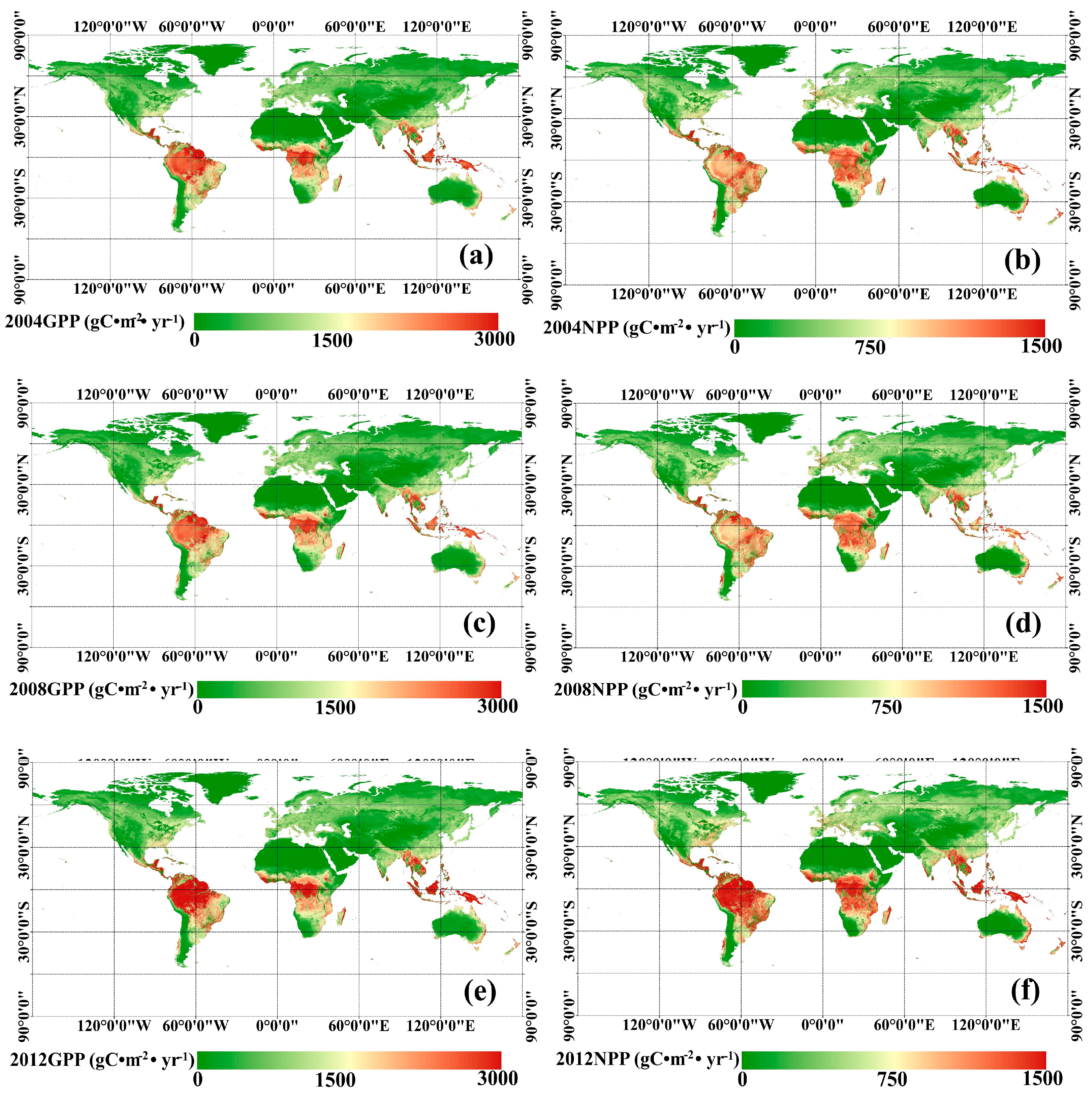
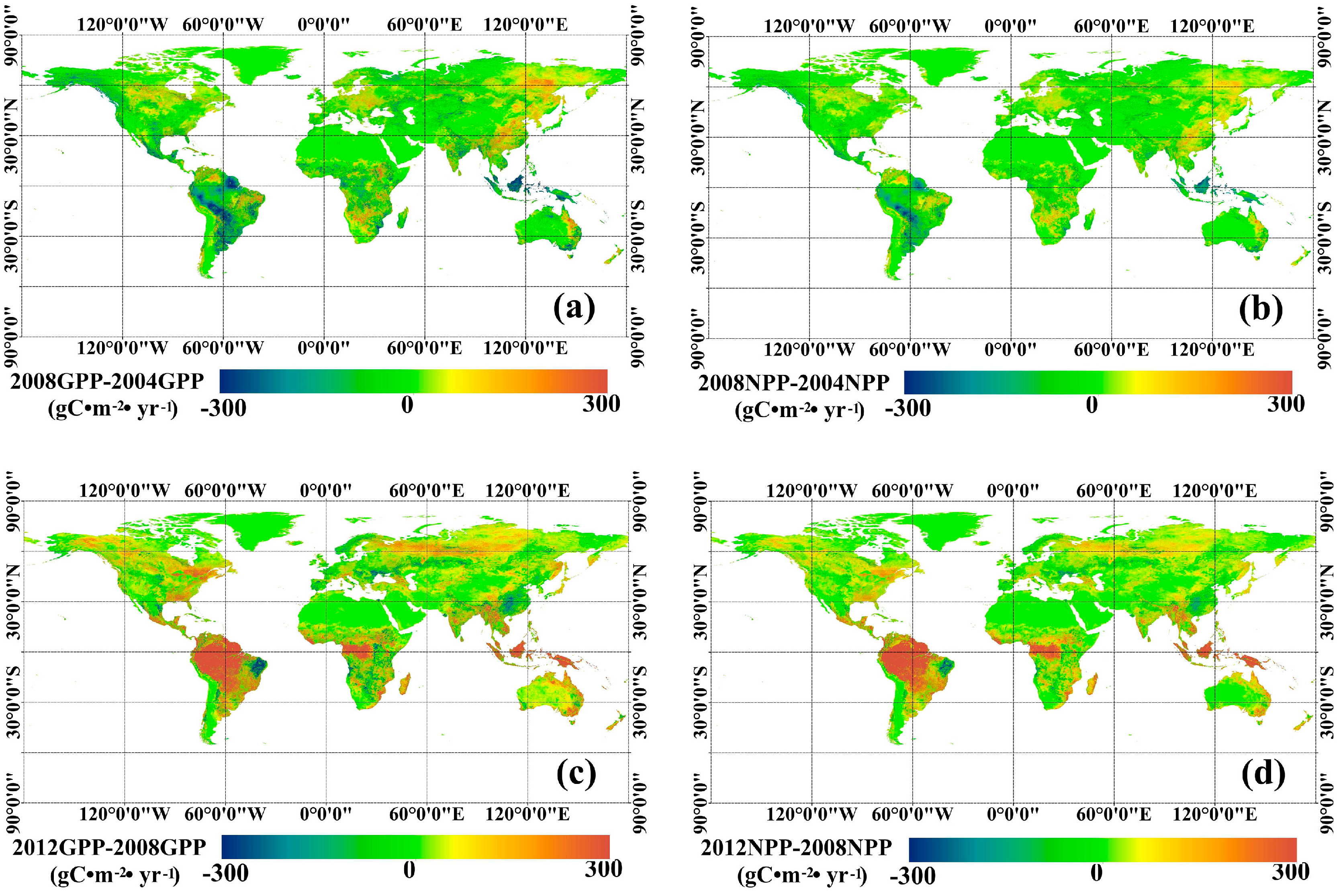
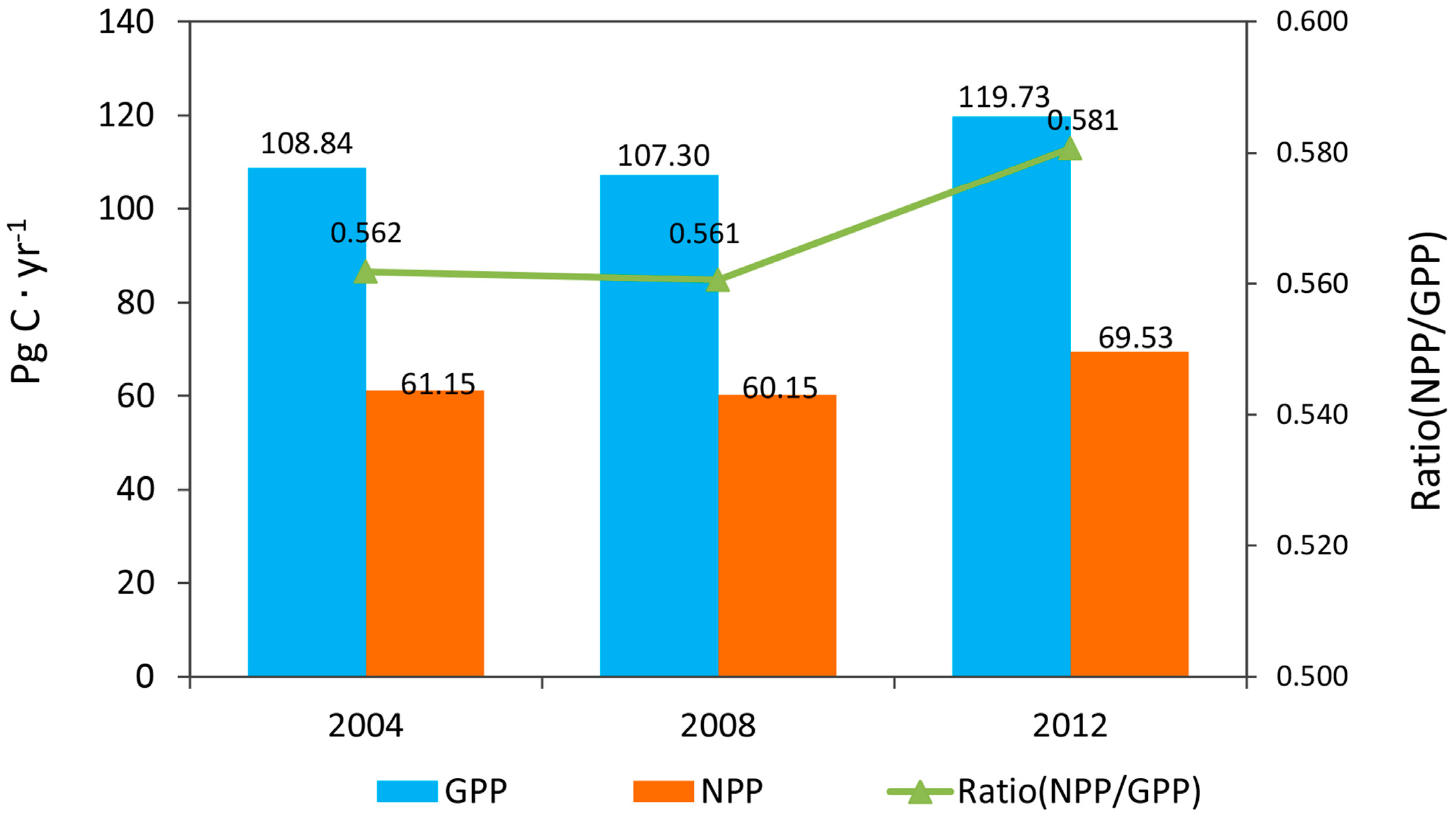
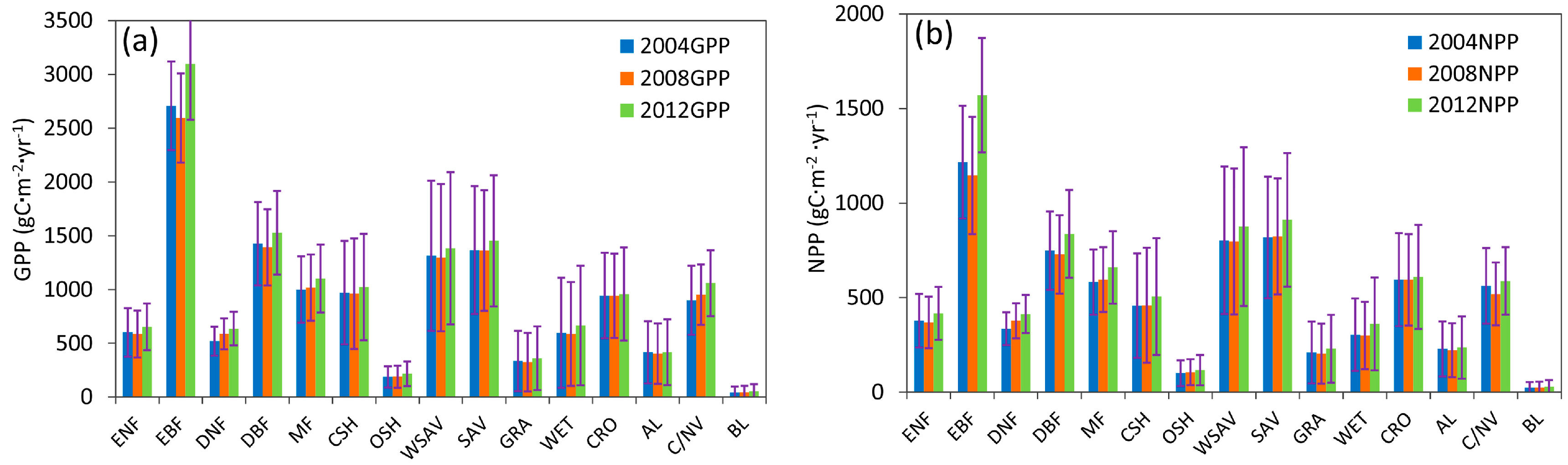
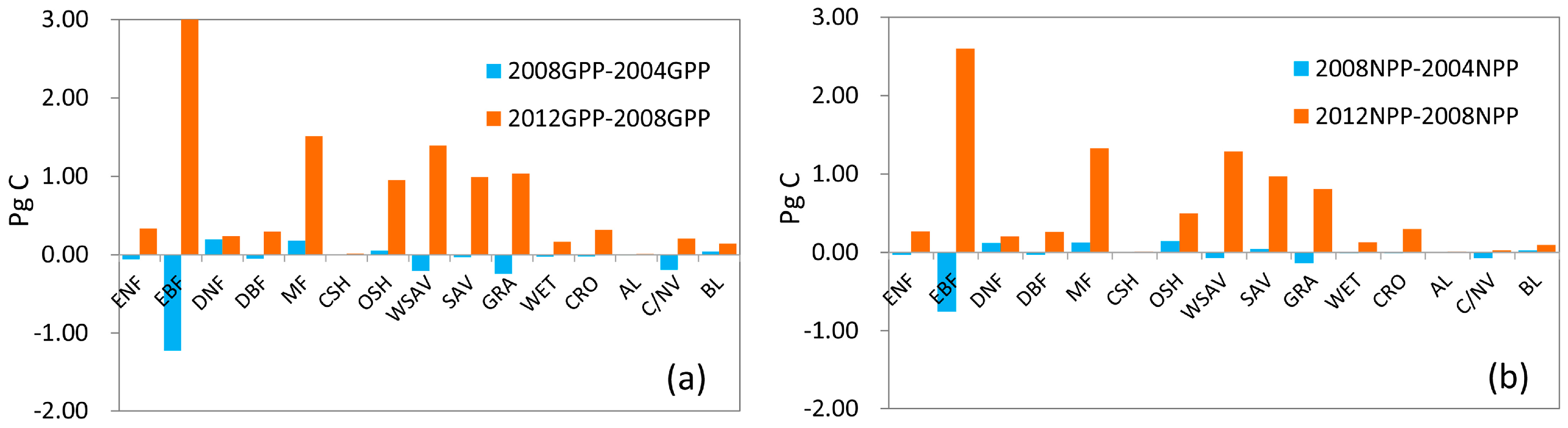
3.1. Temporal and Spatial Variation of Global GPP and NPP

Using the MuSyQ-NPP algorithm, maps of global estimated 1 km GLASS GPP and NPP in 2004, 2008, and 2012 were obtained, as shown in Figure 3. The highest vegetation productivity (GPP > 2000 g C$·$m⁻², NPP > 1000 g C$·$m⁻²) was found in the humid tropic areas, such as Amazonia, Central Africa and South-east Asia, where both temperature and moisture requirements are fully satisfied for photosynthesis. Temperate regions have an intermediate vegetation productivity (GPP $\approx$ 1000–1400 g C$·$m⁻², NPP $\approx$ 500–800 g C$·$m⁻²), and the lowest vegetation productivity (GPP < 400 g C$·$m⁻², NPP < 200 g C$·$m⁻²) was found in either cold or arid regions, where either temperature or precipitation are limiting factors. Variations in GPP and NPP are demonstrated in Figure 4. In general, from 2004 to 2008, few changes occurred in most areas. The largest GPP increases, about 100 g C$·$m⁻², were in Central China and Eastern Russia. In addition, the largest decreases, about 150 g C$·$m⁻², occurred in Amazonia and South-eastern Asia. From 2008 to 2012, GPP and NPP increased in most areas. Specifically, the largest increasing trends occurred in tropic areas, such as Amazonia and South-eastern Asia, in which GPP increased by approximately 400 g C$·$m⁻² and NPP increased approximately by 200 g C$·$m⁻². The next largest increases were seen in areas in Russia, Northern America, and Northeastern China, in which GPP increased by about 100 g C$·$m⁻² and NPP increased by about 50 g C$·$m⁻². The largest decreasing trends occurred in areas of Eastern Brazil, where GPP decreased by about 300 g C$·$m⁻² and NPP decreased by about 150 g C$·$m⁻².

Global total GPP in 2004, 2008 and 2012 was 108.84 Pg C, 107.30 Pg C and 119.73 Pg C, respectively. Global total GPP estimates are comparable with values of 109.29 Pg C [4], 110.5 ± 21.3 Pg C [43] and 132 ± 22 Pg C [1]. Global total GPP decreased 1.41% from 2004 to 2008 and increased 11.58% from 2008 to 2012. Global NPP in 2004, 2008 and 2012 was 61.15 Pg C, 60.15 Pg C and 69.53 Pg C, respectively, which was comparable to previously reported values of 56.40 Pg C [44], 56.02 Pg C [4] and values between 39.9 Pg C and 80.5 Pg C with a mean of 54.9 Pg C [45]. Global total NPP decreased by 1.64% from 2004 to 2008 and increased by 15.59% from 2008 to 2012 according to our study (Figure 5).

The mean and standard deviation of GPP and NPP for different land cover types are shown in Figure 6. GPP and NPP values were highest in EBF. GPP could be as high as 2799.90 g C$·$m⁻²$·$yr⁻¹, and NPP was approximately 1311.29 g C$·$m⁻²$·$yr⁻¹. GPP and NPP values were lowest in Bare Land: GPP was only 47.25 g C$·$m⁻²$·$yr⁻¹, and NPP was only 25.71 g C$·$m⁻²$·$yr⁻¹. Generally, GPP and NPP in 2012 were higher than these in 2004 and 2008 at all land cover types. GPP and NPP in 2008 were at their minimums among these three years. This is more obvious in EBF. GPP was 3097.35 g C$·$m⁻²$·$yr⁻¹ in 2012, 389.76 g C$·$m⁻²$·$yr⁻¹ more than in 2004 and 502.61 g C$·$m⁻²$·$yr⁻¹ more than in 2008. NPP in 2012 could be as high as 1571.14 g C$·$m⁻²$·$yr⁻¹, 354.75 g C$·$m⁻²$·$yr⁻¹ more than in 2004 and 424.82 g C$·$m⁻²$·$yr⁻¹ more than in 2008. However, in DNF, MF, open shrubland (OSH) and bare land (BL), GPP kept increasing from 2004 to 2012. Variation in global total GPP and NPP for all vegetated land cover types is demonstrated in Figure 7. Generally, variations in GPP and NPP from 2004 to 2008 were less than those from 2008 to 2012. The largest variation occurred in the EBF, in which GPP decreased 1.22 Pg C from 2004 to 2008 and increased 3.24 Pg C from 2008 to 2012. The next largest increases were seen in MF, OSH, woody savannas (WSAV), savannas (SAV) and GRA, GPP increased about 1 Pg C, and NPP increased about 0.6 Pg C from 2008 to 2012. The lowest variations were in DNF, DBF, close shrub-land (CSH), CRO, artificial land (AL), cropland/natural vegetation mosaic (C/NV) and BL, in which variations of GPP and NPP were less than 0.2 Pg C. Considering that some of that variability can be explained by regional patterns, we also studied the mean GPP and NPP for different biomes, as well as the variation in GPP and NPP in different biomes (See Text S1 in Supplementary Materials).

3.2. Validation of Estimated GLASS GPP

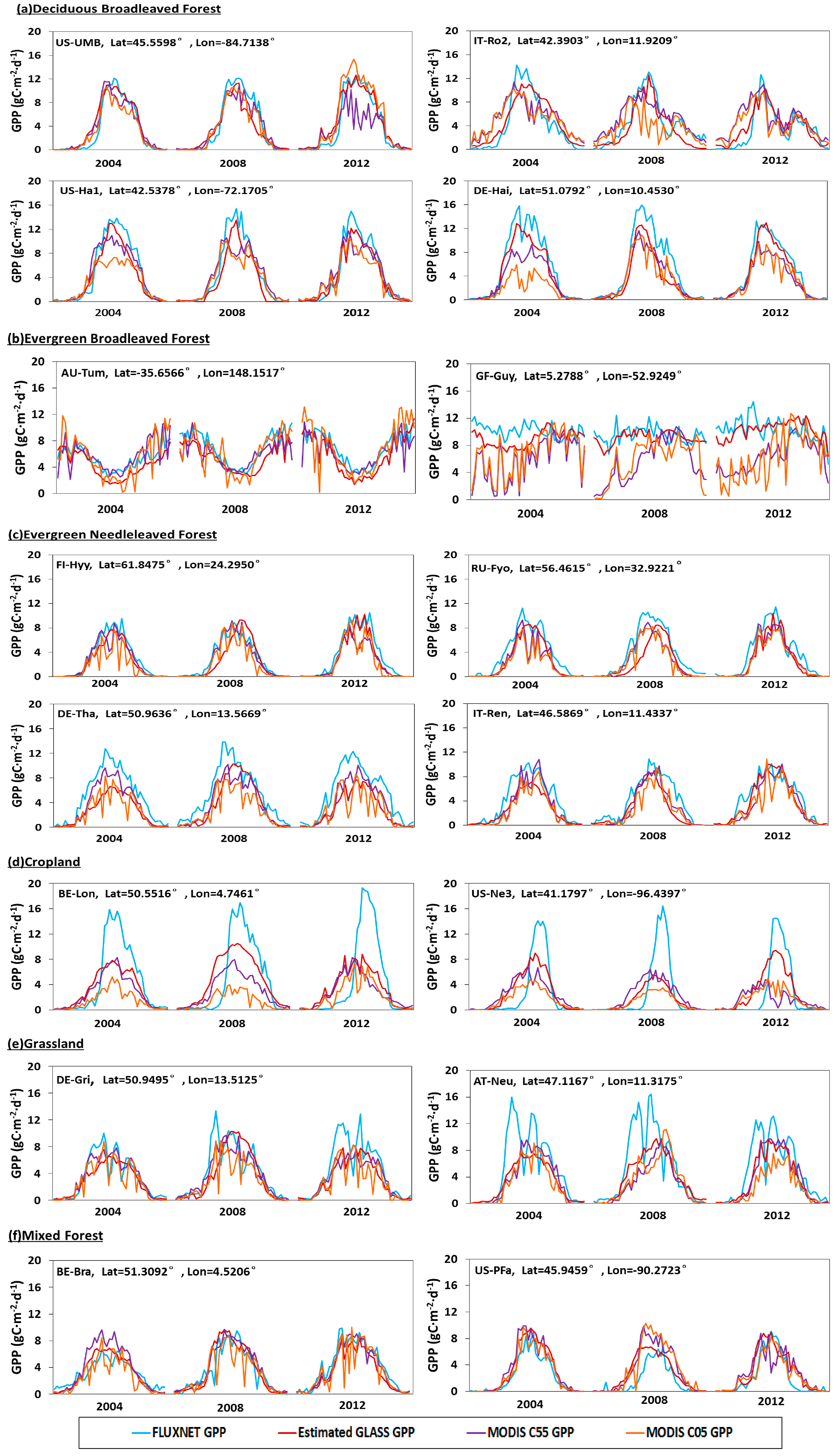
3.2.1. Seasonal Variation in GPP

For various vegetated land cover types, we compared our GPP estimates with eight-day MODIS GPP product and FLUXNET GPP, as shown in Figure 8. With the application of temporal infilling of cloud-contaminated pixels and a consistent forcing meteorology in MODIS revised GPP product (MOD17 C55), we found that the time series of MOD17 C55 GPP was more continuous than the MODIS standard GPP product (MOD17 C05). But, the time series of estimated GLASS GPP in 2004, 2008 and 2012 are clearly more continuous with smoother trajectories than MODIS GPP (both MOD17 C05 GPP and MOD17 C55 GPP), and they agree well with the variations in FLUXNET GPP.

More specifically, the time series of estimated GLASS GPP in deciduous broadleaved forests (DBF) are shown in Figure 8a. It can be clearly seen that estimated GLASS GPP agrees better with FLUXNET GPP than MODIS GPP does and is more continuous, especially during the growing season. At US-Ha1 and De-Hai, estimated GLASS GPP matches much better with the FLUXNET GPP and reflects the peak of the growing season, but MODIS GPP is somewhat underestimated at the peak of the growing season, especially MOD17 C05 GPP in 2004. FLUXNET GPP and estimated GLASS GPP could be as high as 14 g C$·$m⁻²$·$d⁻¹ in the peak of the growing season, but MODIS GPP is much lower, only approximately 8 g C$·$m⁻²$·$d⁻¹.

In evergreen broadleaved forests (EBF), estimated GLASS GPP is obviously more continuous and generally showed better agreement with the FLUXNET GPP, as shown in Figure 8b. FLUXNET GPP showed little seasonal variation at the GF-Guy site, which is located in South America and near the equatorial region. But, at this site, MODIS GPP varied significantly, especially the MOD17 C05 GPP, and was underestimated in the first half of 2004, 2008 and 2012. In 2008 and 2012, MODIS GPP was underestimated most of the time and failed to catch the changes in FLUXNET GPP.

Figure 8c shows the GPP time series in evergreen needle-leaf forests (ENF). Good agreement was achieved between estimated GLASS GPP and FLUXNET GPP, in terms of the absolute values and seasonal trends. Overall, the time series of estimated GLASS GPP was more continuous than MODIS GPP. But at DE-Tha, estimated and MODIS GPP were a little underestimated. In 2008, the estimated growing season was delayed a little compared to the FLUXNET growing season.

Figure 8d demonstrates the GPP time series in croplands (CRO) in 2004, 2008 and 2012. Both MODIS GPP and estimated GLASS GPP significantly underestimated the FLUXNET GPP. Particularly during the growing seasons, estimated GLASS GPP and MODIS GPP were much lower than the FLUXNET GPP. The FLUXNET GPP could be as high as 16 g C$·$m⁻²$·$d⁻¹ at the peak of the growing season, but our estimated GLASS GPP was only approximately 8 g C$·$m⁻²$·$d⁻¹. The MODIS GPP was much less, just about 6 g C$·$m⁻²$·$d⁻¹. But in the fallow season, estimated GLASS GPP and MODIS GPP were higher than the FLUXNET GPP. FLUXNET GPP started to increase rapidly in early June, but the estimated GLASS GPP and MODIS GPP started to increase in March.

In grasslands (GRA), as shown in Figure 8e, peak profiles of FLUXNET GPP appeared in May and July at the DE-Gri and AT-Neu sites. MODIS GPP and estimated GLASS GPP did not reflect these high values. But the matches between the estimated GLASS GPP, MODIS GPP and FLUXNET GPP were very good at other times.

The time series for the estimated GLASS GPP, MODIS GPP and FLUXNET GPP in mixed forests (MF) are displayed in Figure 8f. Generally, estimated GLASS GPP and MODIS GPP could capture the seasonal dynamics of FLUXNET GPP. But estimated and MODIS GPP were a little overestimated during the growing seasons in 2008 and 2012.

In conclusion, estimated GLASS GPP in DBF, EBF, ENF and MF could capture the variations of FLUXNET GPP, and their time series are obviously more continuous with smoother trajectories than MOD17 C05 GPP and MOD17 C55 GPP time series. But in CRO and GRA, estimated GLASS GPP, MOD17 C05 GPP and MOD17 C55 GPP underestimated the FLUXNET GPP during the growing season.

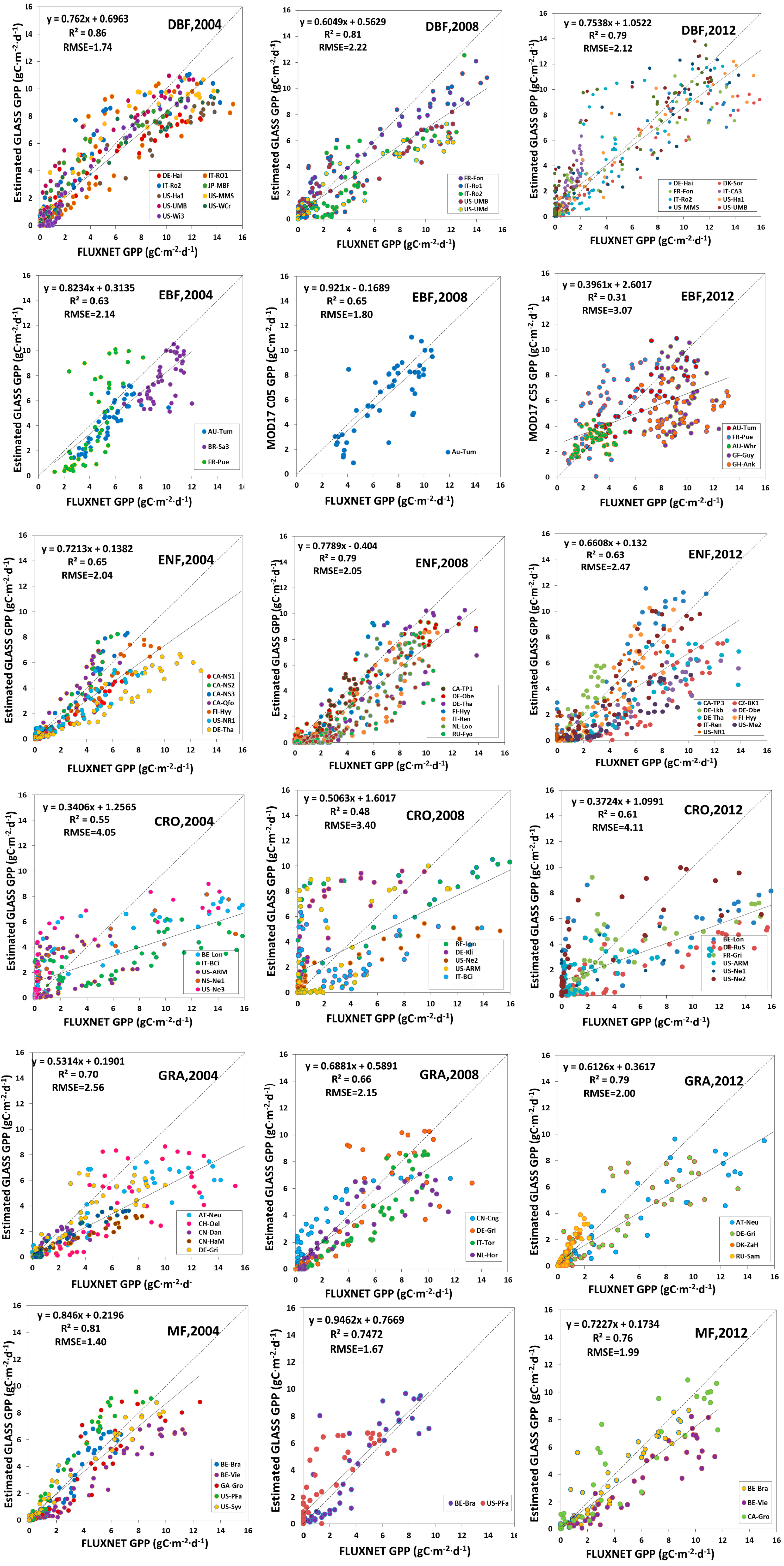
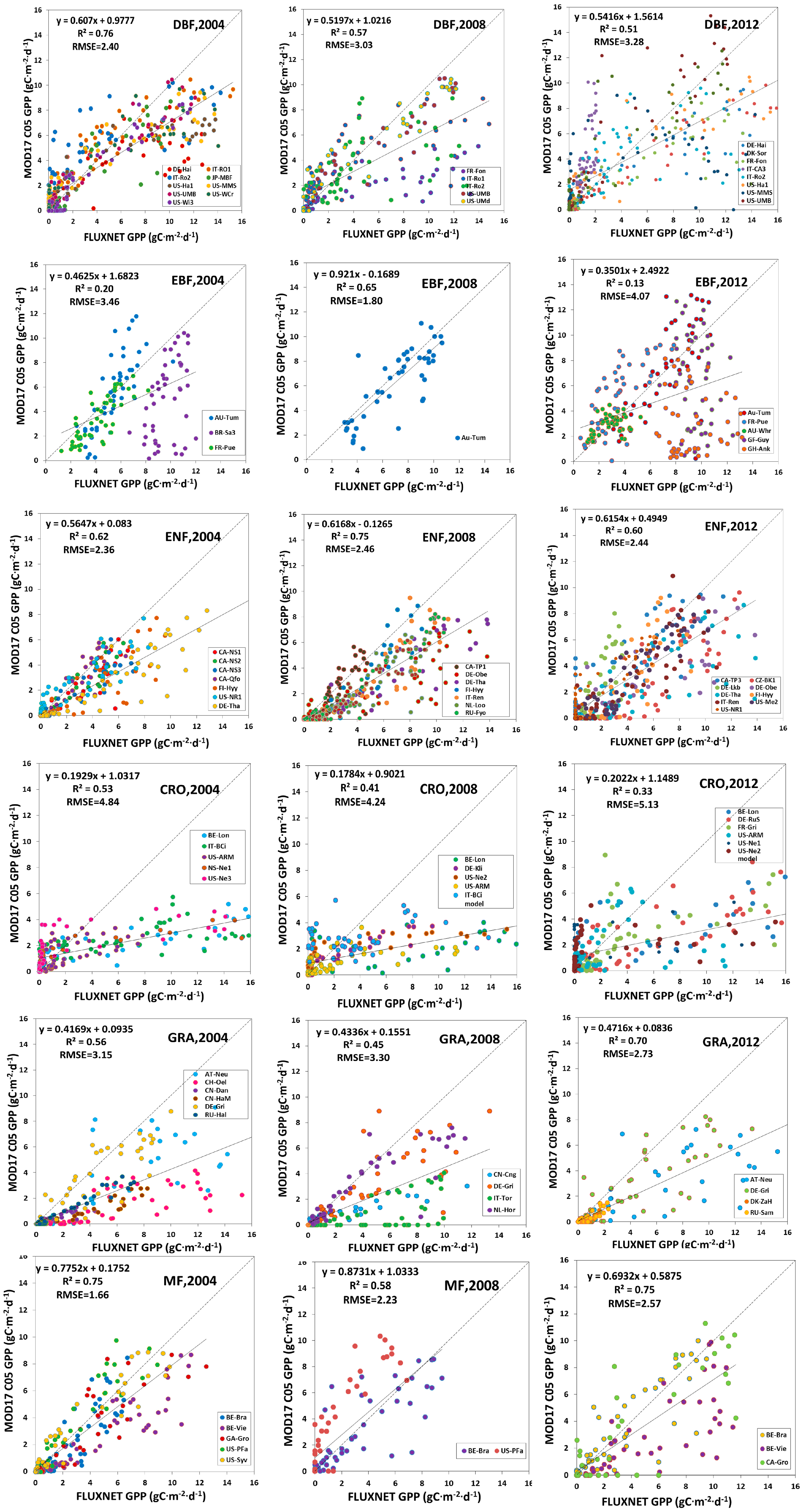
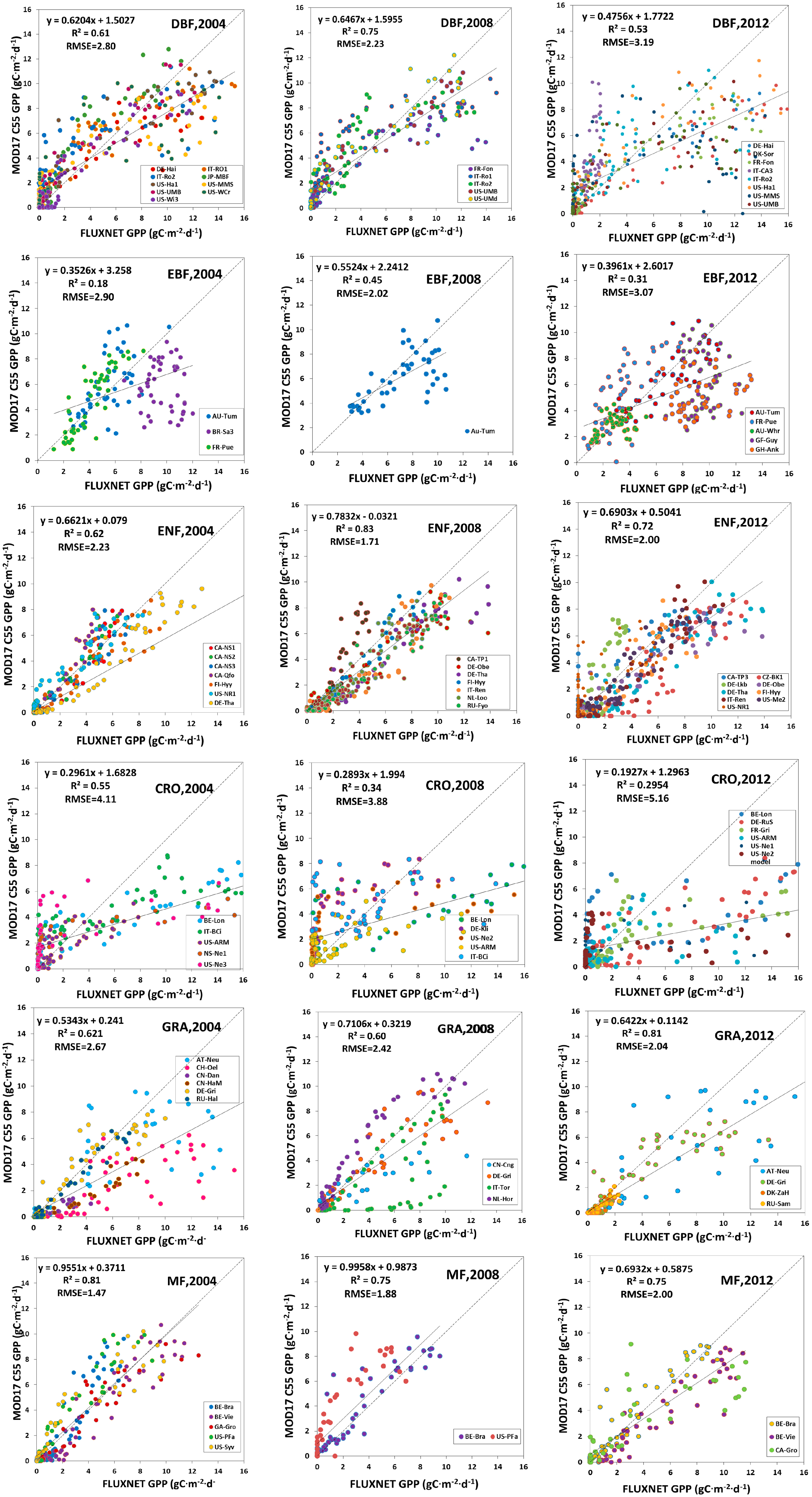
3.2.2. Validation against FLUXNET GPP

Scatter plots between estimated GLASS GPP and FLUXNET GPP, and scatter plots between MODIS GPP (MOD17 C05 GPP and MOD17 C55 GPP) and FLUXNET GPP over different vegetative land cover types were analyzed, as shown in Figure 9, Figure 10 and Figure 11.

R² between estimated GLASS GPP and FLUXNET GPP in DBF could be as high as 0.86 in 2004, 0.81 in 2008 and 0.79 in 2012, and RMSE was 1.74 g C$·$m⁻²$·$d⁻¹ in 2004, 2.22 g C$·$m⁻²$·$d⁻¹ in 2008 and 2.12 g C$·$m⁻²$·$d⁻¹ in 2012. As for the MOD17 C55 GPP, RMSE was 2.80 g C$·$m⁻²$·$d⁻¹ in 2004, 2.23 g C$·$m⁻²$·$d⁻¹ in 2008 and 3.19 g C$·$m⁻²$·$d⁻¹ in 2012. For the MOD15 C05 GPP, RMSE was 2.40 g C$·$m⁻²$·$d⁻¹ in 2004, 3.03 g C$·$m⁻²$·$d⁻¹ in 2008 and 3.28 g C$·$m⁻²$·$d⁻¹ in 2012. The comparison demonstrated that estimated GLASS GPP was more accurate, compared to MODIS GPP (MOD17 C05 GPP and MOD17 C55 GPP) in DBF. In EBF, RMSE between our estimated GLASS GPP and FLUXNET GPP in 2004, 2008 and 2012 were much lower than RMSE between MODIS GPP and FLUXNET GPP. Scatter plots of estimated GLASS GPP were distributed more closely around the 1:1 line, but many MODIS GPP scatter plots are decentralized and are distributed below the 1:1 line. R² between estimated GLASS GPP and FLUXNET GPP could be as high as 0.63, 0.65 and 0.64 in 2004, 2008 and 2012, respectively. But R² between MODIS GPP (MOD17 C05 GPP and MOD17 C55 GPP) and FLUXNET GPP were relative smaller. In ENF, we found that RMSEs between our estimated GLASS GPP and FLUXNET GPP in 2008 and in 2012 are marginally higher than RMSE between MODIS GPP and FLUXNET GPP in 2008 and 2012. In CRO, estimated GLASS GPP and MODIS GPP were much lower than FLUXNET GPP within growing seasons. Therefore, most of the scatter plots were below the 1:1 line, which indicates that both our estimated GLASS GPP and MODIS GPP were underestimated. In GRA, we found that the RMSE was lower between estimated GLASS GPP and FLUXNET GPP than that between MODIS GPP and FLUXNET GPP in 2004. Most scatter plots of MODIS GPP were located under the 1:1 line, which demonstrates that MODIS GPP is underestimated most of the time. In MF, RMSE was lower between estimated GLASS GPP and FLUXNET GPP in 2004 and in 2008. MODIS GPP was overestimated in 2008 at BE-Bra and US-PFa.

In conclusion, we found that RMSE between estimated GLASS GPP and FLUXNET GPP was the smallest in DBF, EBF, CRO, GRA and MF. But in ENF, RMSE between MOD17 C55 GPP and FLUXNET GPP was the smallest. Therefore, estimated GPP achieved the highest precision in DBF, EBF, CRO, GRA and MF.

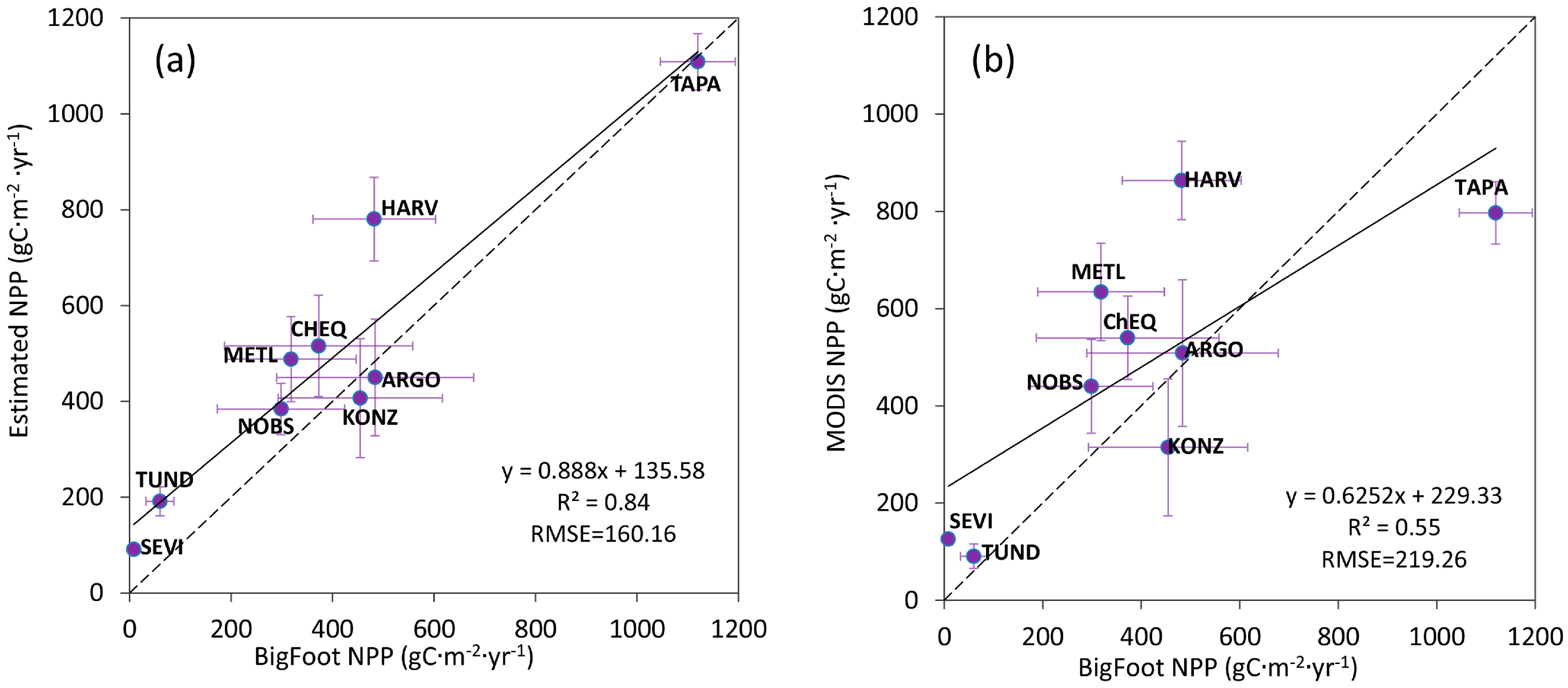
3.3. Validation of Estimated NPP

Time-inconsistencies were found between Bigfoot NPP and our estimation. The Bigfoot NPP data were acquired from 2000 to 2004, but our estimation results are from 2004, 2008 and 2012. To preliminarily validate the model, we calculated the average NPP in 2004, 2008 and 2012 at each Bigfoot site and compared this to the average BigFoot NPP for 2000–2004. In general, a good linear relationship exists between estimated NPP and BigFoot NPP (Figure 12). The R² between estimated NPP and BigFoot NPP was as high as 0.84, and RMSE was 160.16 g C$·$m⁻²$·$yr⁻¹. R² between MODIS NPP and BigFoot NPP was 0.55, and RMSE was 219.26 g C$·$m⁻²$·$yr⁻¹. A higher R² and lower RMSE demonstrate that the estimated NPP achieved a better precision than the MODIS NPP product and indicate the applicability and reliability of the MuSyQ-NPP algorithm in estimating global NPP.

Some studies demonstrate that MODIS products tend towards overestimation of NPP at low productivity sites (such as SEVI) and underestimation at high productivity sites (such as TAPA) [46,47]. Generally, the overestimation appears to be primarily a problem with high MODIS FPAR, and the underestimations are primarily a function of low values for the maximum light use efficiency [46,47]. Scatter plots of estimated NPP in our study were located closer to the 1:1 line (Figure 5), especially at high productivity sites (such as TAPA, KONZ). Overestimates of FPAR at SEVI, METL and CHEQ in midseason contributed to the high MODIS NPP estimates at those sites [46]. Problems with cloud effects on FPAR and LAI estimates also lead to some artificial variation in the MODIS products [46], but the data assimilation framework to generate the GLASS FPAR and LAI products can estimate temporally complete land-surface parameter profiles from time-series reflectance data even if some of the reflectance data are contaminated by residual clouds or missing data [13]. Therefore, NPP estimates at TAPA are more accurate than MODIS NPP.

4. Discussion

4.1. Reasons for GPP Underestimation in Croplands

Estimated GLASS GPP and the MODIS GPP product underestimated and poorly represented FLUXNET GPP, especially in croplands. Estimated GLASS GPP and MODIS GPP were much lower than FLUXNET GPP within growing seasons, but estimated GLASS GPP and MODIS GPP were higher than FLUXNET GPP in non-growing seasons. One of the reasons for these results may be that the potential LUE for crops shows no difference between C3 and C4 species in the algorithm. The C4 crop species have a larger photosynthetic capacity compared to the C3 species; thus, it is necessary to have accurate species-distribution potentials for LUE products in order to determine regional and global estimates of GPP [48]. Second, the height of the eddy covariance instruments, related to the spatial representativeness of the observed carbon flux data, is usually low in croplands, such as BE-Lon and US-Ne3 (about 3.5 m). Scale mismatch exists between ground observed footprint size and satellite-derived footprint size. Thirdly, the problem of mixed pixels may also have an influence on the accuracy of estimated GLASS GPP. Some other types of land cover (such as bare land, grassland and artificial land) may exist in a MODIS 1 km cropland pixel, which may lead to overestimation of FPAR and LAI in the non-growing season, and underestimation of FPAR and LAI in the growing season [49,50]. This might also be the reason for the overestimation of GPP in the non-crop-growth season and underestimation in the crop growth season.

4.2. Limitations in NPP Validation

Site-level validation of MODIS NPP has been more limited because of the logistical constraints of measuring NPP and scaling it to the size of a MODIS grid cell [43,51]. The BigFoot project was designed to provide ground validation data for MODIS land products, including NPP. Thus, the BigFoot data used in this paper to validate GLASS NPP results, varies widely, according site characteristics, i.e., different climate and vegetation types. As BigFoot data are only generated from 2000 to 2004 (Table 1), the problem of time-inconsistency exists when validating the GLASS NPP estimates. To reduce the bias, mean BigFoot NPP in different years (Table 1) were used to validate the estimated mean NPP in 2004, 2008 and 2012. In conclusion, BigFoot NPP could be only used to validate the GLASS NPP estimates preliminarily.

4.3. Future Work

Satellite derived GPP and NPP are difficult to validate, due to the differences in spatial scale between the ground and satellite data. First, the height of the sensors at FLUXNET sites, which is related to the representativeness of the observed data, depends on the type of the vegetation, the extent of fetch, the range of wind velocity and the frequency response of the instrument [51]. Second, the land surface at the site should ideally be flat, with an extensive fetch of uniform vegetation. But in the real environment, many flux tower sites are on undulating or gently sloping terrain, as this is where native vegetation exists [52]. Moreover, some sites consist of mono-specific vegetation (such as cropland and grassland), and others contain a mixture of species. Spatial heterogeneity may lead to some mixed pixels in remote sensing data, therefore, leading to some bias in GPP and NPP estimation and validation. In the future, we may study the spatial representativeness of ground observation data through footprint analysis [53,54,55] and validate the remotely sensed vegetation productivity through the upscaling of ground observation and fine spatial resolution remote sensing data.

Producing accurate estimates of predictions of LUE is another issue that urgently needs to be addressed when estimating vegetation productivity. In this study, the biome-specific potential LUE ${\epsilon }_{max}$ was set at a certain value for each vegetation type. In addition, in this algorithm, actual LUE was calculated based on the assumption that LUE was influenced only by low or high temperatures and water shortages. However, in the real environment, LUE could also be influenced by many other factors, such as the eco-physiological processes in the vegetation, light intensity, and concentrations of CO₂ and O₃ in the atmosphere [56,57]. In addition, LUE shows obvious spatial heterogeneity and temporal variation under the combined influence of vegetation distribution and climate features [58,59,60]. Therefore, accurate predictions of LUE are an important issue should be solved. In the future, we may obtain the spatial distribution of LUE by regression or machine learning methods, such as random forest and support vector machine. Parameter optimization based on process models (such as the Biome-BGC) may be another way to estimate the spatial patterns of LUE. Moreover, relationships between LUE and the fraction of PAR absorbed by chlorophyll (FPARchl) [61] could also be used in LUE estimation.

5. Conclusions

In this paper, global GPP and NPP were firstly estimated with GLASS data using the MuSyQ-NPP algorithm, and an eight-day global GPP and NPP product with a resolution of 1km was developed. Secondly, GLASS GPP/NPP estimates were validated against FLUXNET GPP data and BigFoot NPP data and were compared with MODIS GPP/NPP products. Then, the temporal and spatial variation in global GPP and NPP from 2004 to 2012 was analyzed. Lastly, the advantages of the MuSyQ-NPP algorithm and limitations of this study were discussed. The results of this study indicate that GLASS data and the MuSyQ-NPP algorithm have great potential in regional and global GPP and NPP estimates.

Generally, time series of estimated GLASS GPP in 2004, 2008 and 2012 agreed well with the time series of FLUXNET GPP and MODIS GPP. In addition, the time series of estimated GLASS GPP in our study was more temporally continuous and spatially complete with smoother trajectories compared to MODIS time series. Estimated GLASS GPP matched better with FLUXNET GPP in DBF, EBF, ENF and MF. But in CRO, estimated GLASS GPP and MODIS GPP were lower than FLUXNET GPP within the growing season. Second, estimates of global GPP/NPP in our study achieved higher precision than MODIS GPP/NPP. In DBF, EBF, CRO, GRA and MF, RMSEs were lower between our estimated GLASS GPP and FLUXNET GPP than those between MODIS GPP and FLUXNET GPP. As for NPP, the RMSE between estimated GLASS NPP and BigFoot NPP was only 160.16 g C$·$m⁻²$·$yr⁻¹, much lower than the RMSE between MODIS NPP and BigFoot NPP. Thirdly, the global total GPP decreased by 1.41% from 2004 to 2008 and increased 11.58% from 2008 to 2012. In addition, global NPP decreased by 1.64% from 2004 to 2008 and increased by 15.59% from 2008 to 2012. GPP and NPP in 2012 were higher than in 2004 and 2008 for almost all land cover types. Finally in 2008, GLASS GPP and NPP reached the minimum value of the period analyzed.

References

1. Chen, J.M.; Mo, G.; Pisek, J.; Liu, J.; Deng, F.; Ishizawa, M.; Chan, D. Effects of foliage clumping on the estimation of global terrestrial gross primary productivity. Glob. Biogeochem. Cycles 2012, 26, GB1019. [Google Scholar] [CrossRef]
2. Running, S.W.; Nemani, R.R.; Heinsch, F.A.; Zhao, M.; Reeves, M.; Hashimoto, H. A continuous satellite-derived measure of global terrestrial primary production. AIBS Bull. 2004, 54, 547–560. [Google Scholar] [CrossRef]
3. Heinsch, F.A.; Reeves, M.; Bowker, C.F. User’s Guide, GPP and NPP (MOD 17A2/A3) Products, NASA MODIS Land Algorithm. Available online: https://www.researchgate.net/publication/242118371_User’s_guide_GPP_and_NPP_MOD17A2A3_products_NASA_MODIS_land_algorithm (accessed on 5 December 2017).
4. Zhao, M.; Heinsch, F.A.; Nemani, R.R.; Running, S.W. Improvements of the MODIS terrestrial gross and net primary production global data set. Remote Sens. Environ. 2005, 95, 164–176. [Google Scholar] [CrossRef]
5. Martínez, B.; Camacho, F.; Verger, A.; García-Haro, F.J.; Gilabert, M.A. Intercomparison and quality assessment of MERIS, MODIS and SEVIRI FAPAR products over the Iberian Peninsula. Int. J. Appl. Earth Obs. 2013, 21, 463–476. [Google Scholar] [CrossRef]
6. McCallum, I.; Wagner, W.; Schmullius, C.; Shvidenko, A.; Obersteiner, M.; Fritz, S.; Nilsson, S. Comparison of four global FAPAR datasets over Northern Eurasia for the year 2000. Remote Sens. Environ. 2010, 114, 941–949. [Google Scholar] [CrossRef]
7. Tao, X.; Liang, S.; Wang, D. Assessment of five global satellite products of fraction of absorbed photosynthetically active radiation: Intercomparison and direct validation against ground-based data. Remote Sens. Environ. 2015, 163, 270–285. [Google Scholar] [CrossRef]
8. Ma, H.; Liu, Q.; Liang, S.; Xiao, Z. Simultaneous estimation of leaf area index, fraction of absorbed photosynthetically active radiation, and surface albedo from multiple-satellite data. IEEE Trans. Geosci. Remote Sens. 2017, 55, 4334–4354. [Google Scholar] [CrossRef]
9. Xiao, Z.; Liang, S.; Wang, J.; Chen, P.; Yin, X.; Zhang, L.; Song, J. Use of general regression neural networks for generating the GLASS leaf area index product from time series MODIS surface reflectance. IEEE Trans. Geosci. Remote Sens. 2014, 52, 209–223. [Google Scholar] [CrossRef]
10. Xiao, Z.; Liang, S.; Wang, J.; Xiang, Y.; Zhao, X.; Song, J. Long-time-series global land surface satellite leaf area index product derived from MODIS and AVHRR surface reflectance. IEEE Trans. Geosci. Remote Sens. 2016, 54, 5301–5318. [Google Scholar] [CrossRef]
11. Liang, S.; Zhao, X.; Liu, S.; Yuan, W.; Cheng, X.; Xiao, Z.; Zhang, X.; Liu, Q.; Cheng, J.; Tang, H.; et al. A long-term Global LAnd Surface Satellite (GLASS) data-set for environmental studies. Int. J. Digit. Earth 2013, 6 (Suppl. S1), 5–33. [Google Scholar] [CrossRef]
12. Fang, H.; Jiang, C.; Li, W.; Wei, S.; Baret, F.; Chen, J.; Garcia-Haro, J.; Liang, S.; Liu, R.; Myneni, R.; et al. Characterization and intercomparison of global moderate resolution leaf area index (LAI) products: Analysis of climatologies and theoretical uncertainties. J. Geophys. Res. Biogeogr. 2013, 118, 529–548. [Google Scholar] [CrossRef]
13. Xiao, Z.; Liang, S.; Sun, R.; Wang, J.; Jiang, B. Estimating the fraction of absorbed photosynthetically active radiation from the MODIS data based GLASS leaf area index product. Remote Sens. Environ. 2015, 171, 105–117. [Google Scholar] [CrossRef]
14. Lieth, H. Modeling the primary productivity of the world. In Primary Productivity of the Biosphere; Springer: Berlin/ Heidelberg, Germany, 1975; pp. 237–263. [Google Scholar]
15. Uchijima, Z.; Seino, H. Agroclimatic evaluation of net primary productivity of natural vegetations. J. Agric. Meteorol. 1985, 40, 343–352. [Google Scholar] [CrossRef]
16. Running, S.W.; Thornton, P.E.; Nemani, R.; Glassy, J.M. Global terrestrial gross and net primary productivity from the Earth Observing System. In Methods in Ecosystem Science; Springer: Berlin/ Heidelberg, Germany, 2000; Volume 3, pp. 44–45. [Google Scholar]
17. Potter, C.S.; Randerson, J.T.; Field, C.B.; Matson, P.A.; Vitousek, P.M.; Mooney, H.A.; Klooster, S.A. Terrestrial ecosystem production: A process model based on global satellite and surface data. Glob. Biogeochem. Cycles 1993, 7, 811–841. [Google Scholar] [CrossRef]
18. Prince, S.D.; Goward, S.N. Global primary production: A remote sensing approach. J. Biogeogr. 1995, 22, 815–835. [Google Scholar] [CrossRef]
19. Parton, W.J.; Scurlock, J.M.O.; Ojima, D.S.; Gilmanov, T.G.; Scholes, R.J.; Schimel, D.S.; Kirchner, T.; Menaut, J.-C.; Garcia, M.E.; Kamnalrut, A.; et al. Observations and modeling of biomass and soil organic matter dynamics for the grassland biome worldwide. Glob. Biogeochem. Cycles 1993, 7, 785–809. [Google Scholar] [CrossRef]
20. McGuire, A.D.; Melillo, J.M.; Kicklighter, D.W.; Joyce, L.A. Equilibrium responses of soil carbon to climate change: Empirical and process-based estimates. J. Biogeogr. 1995, 22, 785–796. [Google Scholar] [CrossRef]
21. Running, S.W.; Hunt, E.R., Jr. Generalization of a forest ecosystem process model for other biomes, BIOME-BCG, and an application for global-scale models. In Scaling Physiological Processes; Academic Press: San Diego, CA, USA, 1993; pp. 141–158. [Google Scholar]
22. Cui, T.; Wang, Y.; Sun, R.; Qiao, C.; Fan, W.; Jiang, G.; Hao, L.; Zhang, L. Estimating vegetation primary production in the Heihe River Basin of China with multi-source and multi-scale data. PLoS ONE 2016, 11, e0153971. [Google Scholar] [CrossRef] [PubMed]
23. Running, S.W.; Zhao, M.S. User’s Guide. Daily GPP and Annual NPP (MOD17A2/A3) Products NASA Earth Observing System MODIS Land Algorithm. Version 3.0 for Collection 6. 2015. Available online: https://lpdaac.usgs.gov/sites/default/files/public/product_documentation/mod17_user_guide.pdf (accessed on 5 December 2017).
24. Qiao, C.; Sun, R.; Xu, Z.; Zhang, L.; Liu, L.; Hao, L.; Jiang, G. A study of shelterbelt transpiration and cropland evapotranspiration in an irrigated area in the middle reaches of the Heihe River in northwestern China. IEEE Geosci. Remote Sens. 2015, 12, 369–373. [Google Scholar] [CrossRef]
25. Zhang, K.; Kimball, J.S.; Mu, Q.; Jones, L.A.; Goetz, S.J.; Running, S.W. Satellite based analysis of northern ET trends and associated changes in the regional water balance from 1983 to 2005. J. Hydrol. 2009, 379, 92–110. [Google Scholar] [CrossRef]
26. Priestley, C.H.B.; Taylor, R.J. On the assessment of surface heat flux and evaporation using large-scale parameters. Mon. Weather Rev. 1972, 100, 81–92. [Google Scholar] [CrossRef]
27. Liu, J.; Chen, J.M.; Cihlar, J.; Park, W.M. A process-based boreal ecosystem productivity simulator using remote sensing inputs. Remote Sens. Environ. 1997, 62, 158–175. [Google Scholar] [CrossRef]
28. The GLASS LAI Product at Beijing Normal University. Available online: http://www.bnu-datacenter.com/en (accessed on 5 December 2017).
29. The GLASS LAI Product at the Global Land Cover Facility. Available online: http://glcf.umd.edu (accessed on 5 December 2017).
30. MODIS Land Cover Type/Dynamics. Available online: https://modis.gsfc.nasa.gov/data/dataprod/mod12.php (accessed on 5 December 2017).
31. Channan, S.; Collins, K.; Emanuel, W.R. Global Mosaics of The Standard MODIS Land Cover Type Data; University of Maryland and the Pacific Northwest National Laboratory: College Park, MD, USA, 2014.
32. Xiao, Z.; Wang, T.; Liang, S.; Sun, R. Estimating the fractional vegetation cover from GLASS leaf area index product. Remote Sens. 2016, 8, 337. [Google Scholar] [CrossRef]
33. Carbon Dioxide Information Analysis Center. Available online: http://cdiac.ornl.go (accessed on 5 December 2017).
34. Ruesch, A.; Gibbs, H.K. New IPCC Tier1 Global Biomass Carbon Map for the Year 2000; Carbon Dioxide Information Analysis Center, Oak Ridge National Laboratory: Oak Ridge, TN, USA, 2008.
35. Eggleston, H.S.; Buendia, L.; Miwa, K.; Ngara, T.; Tanabe, K. IPCC Guidelines for National Greenhouse Gas Inventories; Institute for Global Environmental Strategies: Hayama, Japan, 2006. [Google Scholar]
36. Global Land Data Assimilation System. Available online: http://ldas.gsfc.nasa.gov/gldas/GLDASgoals.php (accessed on 5 December 2017).
37. Rodell, M.; Houser, P.R.; Jambor, U.E.A.; Gottschalck, J.; Mitchell, K.; Meng, C.J.; Arenault, K.; Cosgrove, B.; Radakovich, J.; Bosilovich, M.; et al. The global land data assimilation system. Bull. Am. Meteorol. Soc. 2004, 85, 381–394. [Google Scholar] [CrossRef]
38. Fang, H.; Beaudoing, H.K.; Teng, W.L.; Vollmer, B.E. Global Land data assimilation system (GLDAS) products, services and application from NASA hydrology data and information services center (HDISC). In Proceedings of the ASPRS 2009 Annual Conference, Baltimore, MD, USA, 8–13 March 2009. [Google Scholar]
39. Friend, A.D.; Arneth, A.; Kiang, N.Y.; Lomas, M.; Ogee, J.; RÖDENBECK, C.; Running, S.W.; Santaren, J.; Sitch, S.; Viovy, N.; et al. FLUXNET and modelling the global carbon cycle. Glob. Chang. Biol. 2007, 13, 610–633. [Google Scholar] [CrossRef]
40. Knorr, W.; Kattge, J. Inversion of terrestrial ecosystem model parameter values against eddy covariance measurements by Monte Carlo sampling. Glob. Chang. Biol. 2005, 11, 1333–1351. [Google Scholar] [CrossRef]
41. Fluxdata. Available online: http://fluxnet.fluxdata.org (accessed on 5 December 2017).
42. Cohen, W.B.; Turner, D.P.; Gower, S.T.; Running, S.W. Linking In Situ Measurements, Remote Sensing, and Models to Validate MODIS Products Related to the Terrestrial Carbon Cycle. NASA Terrestrial Ecology Program. 2009. Available online: http://www.fsl.orst.edu/larse/bigfoot/index.html (accessed on 5 December 2017).
43. Yuan, W.; Liu, S.; Yu, G.; Bonnefond, J.M.; Chen, J.; Davis, K.; Desai, A.R.; Goldstein, A.H.; Gianelle, D.; Rossi, F.; et al. Global estimates of evapotranspiration and gross primary production based on MODIS and global meteorology data. Remote Sens. Environ. 2010, 114, 1416–1431. [Google Scholar] [CrossRef]
44. Field, C.B.; Behrenfeld, M.J.; Randerson, J.T.; Falkowski, P. Primary production of the biosphere: Integrating terrestrial and oceanic components. Science 1998, 281, 237–240. [Google Scholar] [CrossRef] [PubMed]
45. Cramer, W.; Kicklighter, D.W.; Bondeau, A.; Moore, B., III; Churkina, G.; Nemry, B.; Ruimy, A.; Schloss, A.L.; Model, P.O.T.P.N. Comparing global models of terrestrial net primary productivity (NPP): Overview and key results. Glob. Chang. Boil. 1999, 5, 1–15. [Google Scholar] [CrossRef]
46. Turner, D.P.; Ritts, W.D.; Cohen, W.B.; Maeirsperger, T.K.; Gower, S.T.; Kirschbaum, A.A.; Running, S.W.; Zhao, M.; Wofsy, S.C.; Dunn, A.L.; et al. Site-level evaluation of satellite-based global terrestrial gross primary production and net primary production monitoring. Glob. Chang. Biol. 2005, 11, 666–684. [Google Scholar] [CrossRef]
47. Turner, D.P.; Ritts, W.D.; Cohen, W.B.; Gower, S.T.; Running, S.W.; Zhao, M.; Costa, M.H.; Kirschbaum, A.A.; Ham, J.M.; Saleska, S.R.; et al. Evaluation of MODIS NPP and GPP products across multiple biomes. Remote Sens. Environ. 2006, 102, 282–292. [Google Scholar] [CrossRef]
48. Yuan, W.; Cai, W.; Nguy-Robertson, A.L.; Fang, H.; Suyker, A.E.; Chen, Y.; Dong, W.; Liu, S.; Zhang, H. Uncertainty in simulating gross primary production of cropland ecosystem from satellite-based models. Agric. For. Meteorol. 2015, 207, 48–57. [Google Scholar] [CrossRef]
49. Zhang, Y.; Yu, Q.; Jiang, J.I.E.; Tang, Y. Calibration of Terra/MODIS gross primary production over an irrigated cropland on the North China Plain and an alpine meadow on the Tibetan Plateau. Glob. Chang. Biol. 2008, 14, 757–767. [Google Scholar] [CrossRef]
50. Zhang, Q.; Cheng, Y.B.; Lyapustin, A.I.; Wang, Y.; Gao, F.; Suyker, A.; Verma, S.; Middleton, E.M. Estimation of crop gross primary production (GPP): FAPAR chl versus MOD15A2 FPAR. Remote Sens. Environ. 2014, 153, 1–6. [Google Scholar] [CrossRef]
51. Turner, D.P.; Ollinger, S.; Smith, M.L.; Krankina, O.; Gregory, M. Scaling net primary production to a MODIS footprint in support of earth observing system product validation. Int. J. Remote Sens. 2004, 25, 1961–1979. [Google Scholar] [CrossRef]
52. Olson, R.J.; Holladay, S.K.; Cook, R.B.; Falge, E.; Baldocchi, D.; Gu, L. FLUXNET. Database of Fluxes, Site Characteristics, and Flux-Community Information; Oak Ridge National Laboratory (ORNL): Oak Ridge, TN, USA, 2004.
53. Schuepp, P.H.; Leclerc, M.Y.; Macpherson, J.I.; Desjardins, R.L. Footprint prediction of scalar fluxes from analytical solutions of the diffusion equation. Bound. Layer Meteorol. 1990, 50, 353–373. [Google Scholar] [CrossRef]
54. Sogachev, A.; Menzhulin, G.V.; Heimann, M.; Lloyd, J. A simple three-dimensional canopy—Planetary boundary layer simulation model for scalar concentrations and fluxes. Tellus B 2002, 54, 784–819. [Google Scholar]
55. Chen, B.; Ge, Q.; Fu, D.; Yu, G.; Sun, X.; Wang, S.; Wang, H. Data-model fusion approach for upscaling gross ecosystem productivity to the landscape scale based on remote sensing and flux footprint modeling. Biogeosciences 2010, 7, 2943–2958. [Google Scholar] [CrossRef] [Green Version]
56. Green, D.S.; Erickson, J.E.; Kruger, E.L. Foliar morphology and canopy nitrogen as predictors of light-use efficiency in terrestrial vegetation. Agric. For. Meteorol. 2003, 115, 163–171. [Google Scholar] [CrossRef]
57. Van Oijen, M.; Dreccer, M.F.; Firsching, K.H.; Schnieders, B.J. Simple equations for dynamic models of the effects of CO2 and O3 on light-use efficiency and growth of crops. Ecol. Model. 2004, 179, 39–60. [Google Scholar] [CrossRef]
58. Turner, D.P.; Gower, S.T.; Cohen, W.B.; Gregory, M.; Maiersperger, T.K. Effects of spatial variability in light use efficiency on satellite-based NPP monitoring. Remote Sens. Environ. 2002, 80, 397–405. [Google Scholar] [CrossRef]
59. Ito, A.; Oikawa, T. Global Mapping of Terrestrial Primary Productivity and Light-Use Efficiency with a Process-Based Model; Global Environmental Change in the Ocean and on Land, Terrapub: Tokyo, Japan, 2004; pp. 343–358. [Google Scholar]
60. Still, C.J.; Randerson, J.T.; Fung, I.Y. Large-scale plant light-use efficiency inferred from the seasonal cycle of atmospheric CO2. Glob. Chang. Biol. 2004, 10, 1240–1252. [Google Scholar] [CrossRef]
61. Xiao, X. Light absorption by leaf chlorophyll and maximum light use efficiency. IEEE Trans. Geosci. Remote Sens. 2006, 44, 1933–1935. [Google Scholar] [CrossRef]
Figure 1. Flowchart of gross primary production (GPP) and net primary production (NPP) estimation and validation. FPAR: Fraction of Photosynthetically Active Radiation; LAI: Leaf Area Index; LUE: Light Use Efficiency; PAR: Photosynthetically Active Radiation; APAR: Absorbed Photosynthetically Active Radiation; DEM: Digital Elevation Model.
Remotesensing 10 00327 g001
Figure 2. MODerate Resolution Imaging Spectroradiometer (MODIS) International Geosphere Biosphere Program (IGBP) land-cover and location of FLUXNET sites and BigFoot sites.
Remotesensing 10 00327 g002
Figure 3. Global 1 km GPP and NPP in 2004, 2008 and 2012: (a) global GPP in 2004; (b) global NPP in 2004; (c) global GPP in 2008; (d) global NPP in 2008; (e) global GPP in 2012; (f) global NPP in 2012.
Remotesensing 10 00327 g003
Figure 4. Variations in global GPP and NPP from 2004 to 2012: (a) variation in GPP from 2004 to 2008; (b) variation in NPP from 2004 to 2008; (c) variation in GPP from 2008 to 2012; (d) variation in NPP from 2008 to 2012.
Remotesensing 10 00327 g004
Figure 5. Global GPP and NPP in 2004, 2008 and 2012 estimated using Global LAnd Surface Satellite (GLASS) data.
Remotesensing 10 00327 g005
Figure 6. Global mean and standard deviations of GPP and NPP for all vegetated land cover types: (a) global mean and standard deviations of GPP; (b) global mean and standard deviations of NPP.
Remotesensing 10 00327 g006
Figure 7. Variation in global total GPP and NPP for all vegetated land cover types: (a) variation in global GPP; (b) variation in global NPP.
Remotesensing 10 00327 g007
Figure 8. Seasonal variation in the estimated GLASS GPP, FLUXNET GPP, MOD17 C05 GPP and MOD17 C55 GPP for several sites with different vegetation types.
Remotesensing 10 00327 g008
Figure 9. Validation of estimated GLASS GPP against FLUXNET GPP.
Remotesensing 10 00327 g009
Figure 10. MODIS C05 GPP validation against FLUXNET GPP.
Remotesensing 10 00327 g010
Figure 11. MODIS C55 GPP validation against FLUXNET GPP.
Remotesensing 10 00327 g011
Figure 12. Validation of estimated GLASS NPP and MODIS NPP against BigFoot NPP: (a) validation of estimated GLASS NPP against BigFoot NPP; (b) validation of MODIS NPP against BigFoot NPP. x is the average of BigFoot NPP, the years being averaged are shown in Table 1; y is the average of NPP in 2004, 2008 and 2012.
Remotesensing 10 00327 g012