Article

Estimating Tree Position, Diameter at Breast Height, and Tree Height in Real-Time Using a Mobile Phone with RGB-D SLAM

1
Precision Forestry Key Laboratory of Beijing, Beijing Forestry University, Beijing 100083, China
2
School of Nature Conservation, Beijing Forestry University, Beijing 100083, China
3
College of Forestry, Beijing Forestry University, Beijing 100083, China
*
Author to whom correspondence should be addressed.
Remote Sens. 2018, 10(11), 1845; https://doi.org/10.3390/rs10111845
Submission received: 8 October 2018 / Revised: 1 November 2018 / Accepted: 19 November 2018 / Published: 21 November 2018
(This article belongs to the Special Issue Aerial and Near-Field Remote Sensing Developments in Forestry)

Abstract

:
Accurate estimation of tree position, diameter at breast height (DBH), and tree height measurements is an important task in forest inventory. Mobile Laser Scanning (MLS) is an important solution. However, the poor global navigation satellite system (GNSS) coverage under the canopy makes the MLS system unable to provide globally-consistent point cloud data, and thus, it cannot accurately estimate the forest attributes. SLAM could be an alternative for solutions dependent on GNSS. In this paper, a mobile phone with RGB-D SLAM was used to estimate tree position, DBH, and tree height in real-time. The main aims of this paper include (1) designing an algorithm to estimate the DBH and position of the tree using the point cloud from the time-of-flight (TOF) camera and camera pose; (2) designing an algorithm to measure tree height using the perspective projection principle of a camera and the camera pose; and (3) showing the measurement results to the observer using augmented reality (AR) technology to allow the observer to intuitively judge the accuracy of the measurement results and re-estimate the measurement results if needed. The device was tested in nine square plots with 12 m sides. The tree position estimations were unbiased and had a root mean square error (RMSE) of 0.12 m in both the x-axis and y-axis directions; the DBH estimations had a 0.33 cm (1.78%) BIAS and a 1.26 cm (6.39%) root mean square error (RMSE); the tree height estimations had a 0.15 m (1.08%) BIAS and a 1.11 m (7.43%) RMSE. The results showed that the mobile phone with RGB-D SLAM is a potential tool for obtaining accurate measurements of tree position, DBH, and tree height.

Graphical Abstract

1. Introduction

Forest ecosystems are considered important for the survival of both animals and human beings because of their environmental and socio-economic benefits. They not only provide services such as soil and water conservation, carbon storage, climate regulation, and biodiversity, but also provide food, wood, and energy [1,2,3]. Forest resource information is an important solid basis for making decisions at different levels according to various needs such as timber harvesting, biomass, species diversity, watershed protection, and climate change impact evaluation, etc. [4]. Forest inventory primarily involves the collection of forest resource information, which aims to provide accurate estimates of the forest characteristics including the wood volume, biomass, or species diversity within the region of interest [5]. These attributes are precisely estimated by models constructed using tree species, diameter at breast height (DBH), and tree height [6]. The conventional instruments used to measure these properties are calipers and clinometers for the DBH and tree heights, respectively [6,7].
Forest inventory has gradually improved with the advancement of remote sensing sensor technology, computing capabilities, and Internet of Things (IoT) [8,9,10,11]. New technologies with high levels of precision and accuracy in the field of forestry have been introduced in recent years [12]. Terrestrial laser scanning (TLS), also known as ground-based Light Detection and Ranging (LiDAR), provides a solution for efficiently collecting the reference data. This technology has been used to extract various forestry attributes [6,13,14,15,16]. However, the TLS has some operational and performance limitations, especially when it is used in large forests, as it is time consuming, laborious, and intensive to carry and mount [17]; moreover, its data processing is also difficult [15]. Mobile Laser Scanning (MLS) is a vehicle born system with an inertial navigation system (INS) and a laser scanner, which makes it possible to move and measure 6 degrees-of-freedom (DOF) of the laser scanner in forests [17,18,19,20,21]. However, the poor GNSS coverage under the canopy could hinder the positioning accuracy, hence making it difficult to achieve a globally-consistent point cloud [22]. Simultaneous localization and mapping (SLAM) is a process that can simultaneously generate the map of unfamiliar environmental conditions, as well as locating the mobile platform [23,24]. This technology is a potential solution that can use sensors such as cameras and lasers to perform relative positioning without GNSS signals through SLAM algorithms in real-time. Some previous studies initially applied SLAM to the forestry inventory process [22,25,26,27]. However, the MLS system is relatively complex, heavy, and expensive.
The Time of Flight (TOF) camera is an alternative to LiDAR, and its basic principle is its consistency with LiDAR. The difference is that TOF cameras generally use infrared as the light source, and do not use point-by-point scanning, but rather, an integrated matrix of multiple TOF sensors to measure multiple distances simultaneously [28]. TOF cameras are power efficient and smaller than LiDARs, and can even be integrated into a mobile phone [29]. The combination of the TOF camera and RGB camera forms an RGB-D camera that can acquire the texture and depth information of the surrounding environment, and it is often used as input to the SLAM system which known as the RGB-D SLAM system [30]. This sensor overcomes the shortcomings of the inability of a monocular SLAM system to obtain the scale and correspondence of a stereo SLAM [30]. With the improvement of the SLAM algorithm and the advancement of chip computing capabilities, the RGB-D SLAM system can even run on a mobile phone [29]. Compared to the traditional MLS system, the mobile phone has the advantages of being portable, inexpensive, and highly integrated. Previously, researchers mainly used the SLAM algorithm to improve the pose estimation accuracy of the MLS system offline [25,26,27,31]. Some other researchers also used point clouds from RGB-D SLAM to obtain tree positions and DBHs offline instead of emphasizing real-time access to forest attributes [32,33]. This paper aims to estimate forest attributes in real-time in a forest inventory using a mobile phone with RGB-D SLAM. We design algorithms for the mobile phone with RGB-D SLAM, to evaluate tree position, DBH, and tree height in forests online. In addition, AR technology is used to display the estimated results on the screen of a mobile phone, enabling the observer to visually evaluate their accuracy.
This paper is organized as follows. The SLAM algorithms and the technology of the portable SLAM device used in this paper are described in Section 2. Section 3 describes the study material, the designed system flow, and the algorithms involved in the estimation process. Section 4 provides the experimental results for nine field plots. Section 5 discusses the results through comparison with previous studies. Section 6 is the conclusions.

2. Theory and Technology
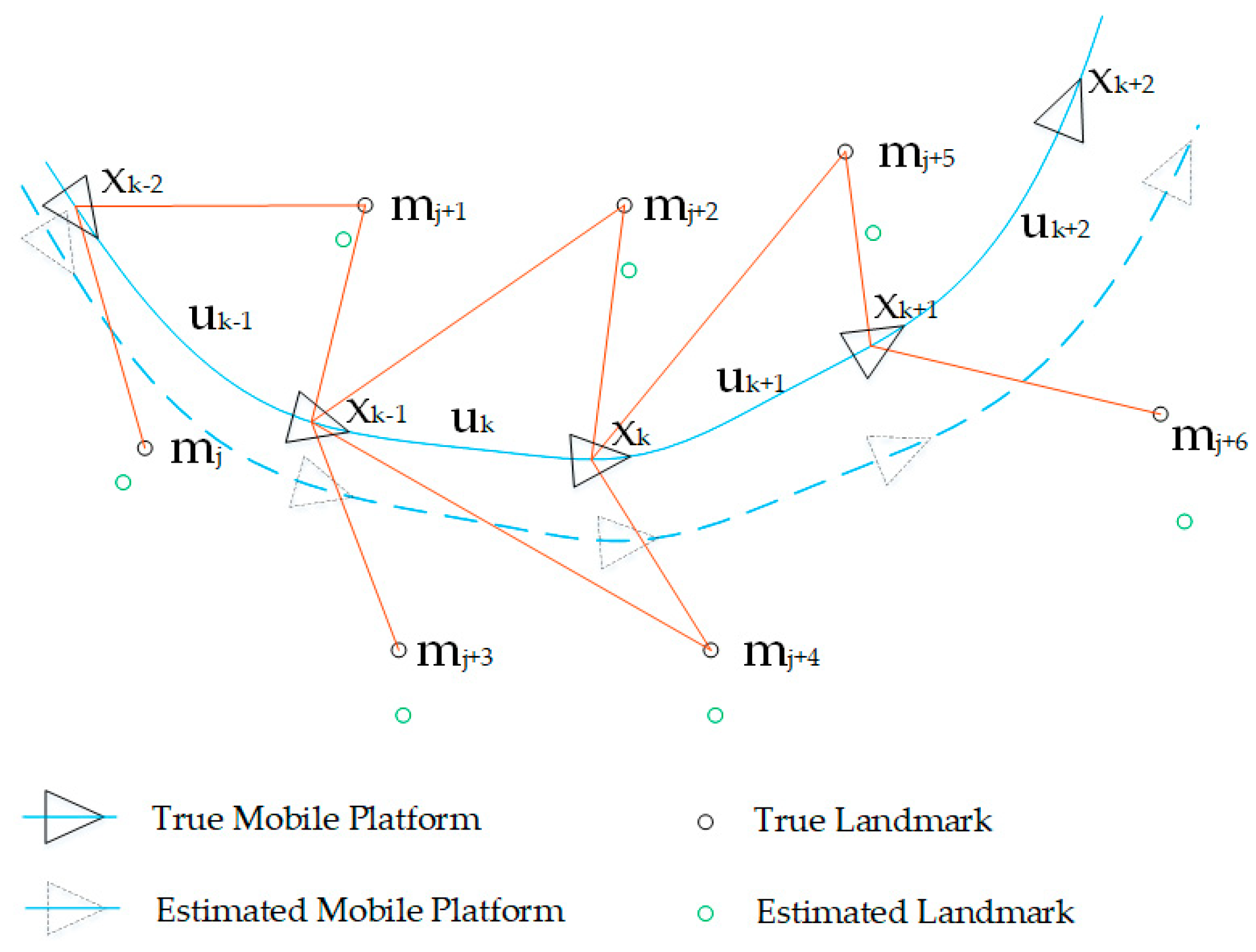
2.1. SLAM

SLAM is the process by which a mobile platform builds a map of the surrounding environment and finds its location using the map in real-time, as shown in Figure 1.
A mobile platform moves in an unknown area and, at the same time, separately observes the surrounding unknown landmarks and records their relative motion through the mounted visual sensors and motion sensors. Then, the relative positions of the landmarks and the pose of the mobile platform are estimated in real time. In probabilistic form, data from motion sensors u k are described as a motion model (a probability distribution):
  P ( x k | x k 1 ,   u k ) .  
Here, x k , x k 1 are the platform poses at times k and k − 1, respectively. Data from the vision sensors z k are described as an observation model (a probability distribution):
  P ( z k | x k ,   m ) .  
Here, m is the set of all landmarks. Generally, the SLAM problem is best described as a probabilistic Markov chain. That is, the joint posterior probability at time k, P ( x k , m | Z 0 : k , U 0 : k ,   x 0 ) , is solved using the posterior joint probability at time k − 1, P ( x k 1 , m | Z 0 : k 1 , U 0 : k 1 ,   x 0 ) , and some other conditions. In the SLAM algorithm, this is implemented using recursive steps, namely, predictive update and observation update forms:
Predictive update
  P ( x k , m | Z 0 : k 1 , U 0 : k ,   x 0 ) = P ( x k | x k 1 , u k ) P ( x k 1 , m | Z 0 : k 1 , U 0 : k 1 ,   x 0 ) d x k 1  
Observation update
  P ( x k , m | Z 0 : k , U 0 : k ,   x 0 ) = P ( z k | x k , m ) P ( x k , m | Z 0 : k 1 , U 0 : k ,   x 0 ) P ( z k | Z 0 : k 1 , U 0 : k )  
Obviously, the key to solving the SLAM problem is to give a reasonable expression of the motion model and the observation model, and then the predictive update and observation update are used to solve the target probability distribution. Three commonly-used methods for solving SLAM problems are extended Kalman filtering (EKF), sparse nonlinear optimization, and particle filtering.

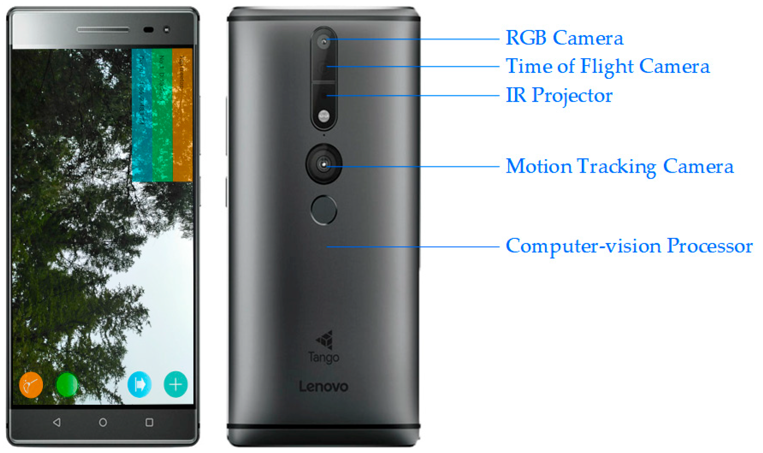
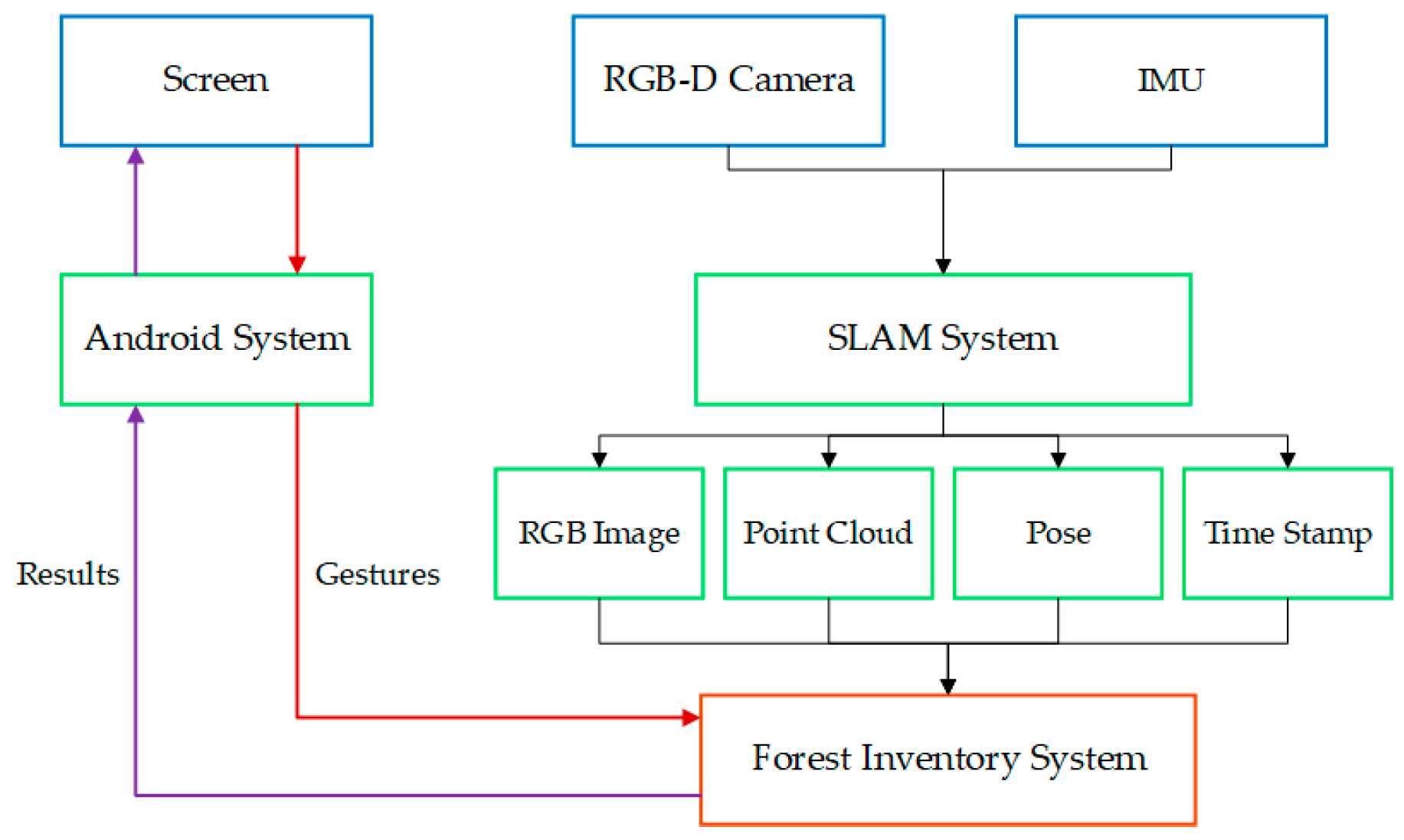
2.2. The Technology of a Portable Graph-SLAM Device

SLAM algorithms have been implemented to track device positions in real-time to build maps of the surrounding three-dimensional (3D) world. Though most SLAM software today works only on high powered computers, Project Tango [29] enables this technology to run on a portable mobile platform (Smartphone). Project Tango created a technology that enables mobile devices to acquire their poses in the three-dimensional world in real time using highly customized hardware and software. Three-dimensional maps can also be constructed by combining pose data with texture and depth information.
Figure 2 shows the smartphone with Google Tango sensors (Lenovo Phab 2 Pro [31]) which was used in this paper. The mobile phone contains a combination of an RGB camera, a time of flight camera, and a motion-tracking camera called a vision sensor. The sensor is used to acquire texture and depth information of the 3D world so that the phone has a similar perspective of the real world. A 9-axis acceleration/gyroscope/compass sensor combined with the vision sensor can be used to implement a Visual-Inertial Odometer system using SLAM algorithms. Some special hardware, such as a computer-vision processor, is used to help speed up data processing so that the pose of the device can be acquired and adjusted in real-time.
The device uses a Visual-Inertial Odometer system for the front end and back end optimization algorithms implement adjustments to account for odometry drift. These adjustments are mainly done through pose graph non-linear optimization and loop closure optimization. These optimizations use visual features to identify previously-visited regions and then adjust the corresponding camera pose drift during this process.

3. Materials and Methods
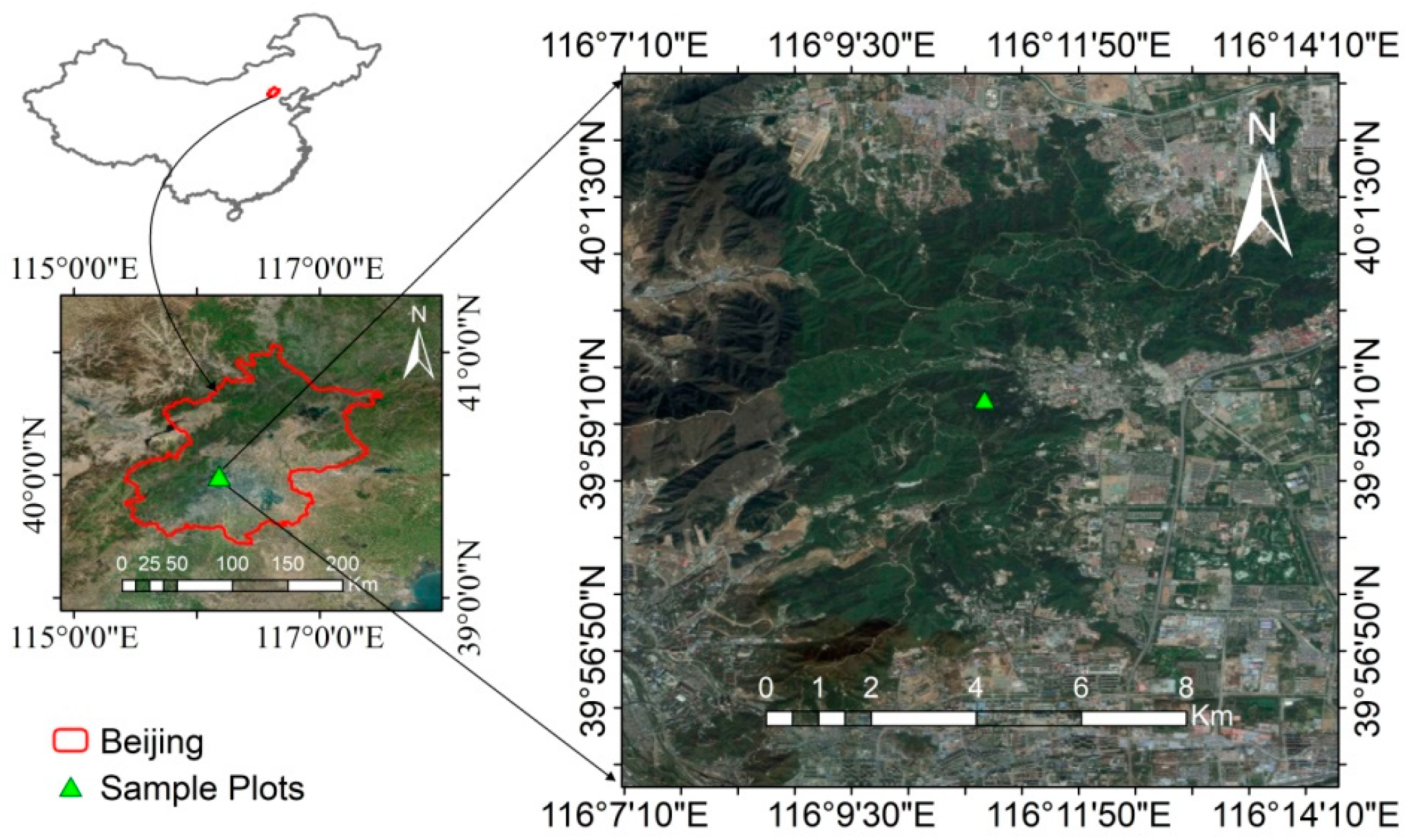
3.1. Study Area

This study was conducted in a managed forest located in the suburbs of Beijing, China (N39°59′ E116°11′, Figure 3). We took nine (12 m × 12 m) square plots based on a wide range of DBH and tree height values. The selected plots had fewer shrubs and were accessible to locals. Table 1 presents the summarized basic description of the plots.

3.2. Methods

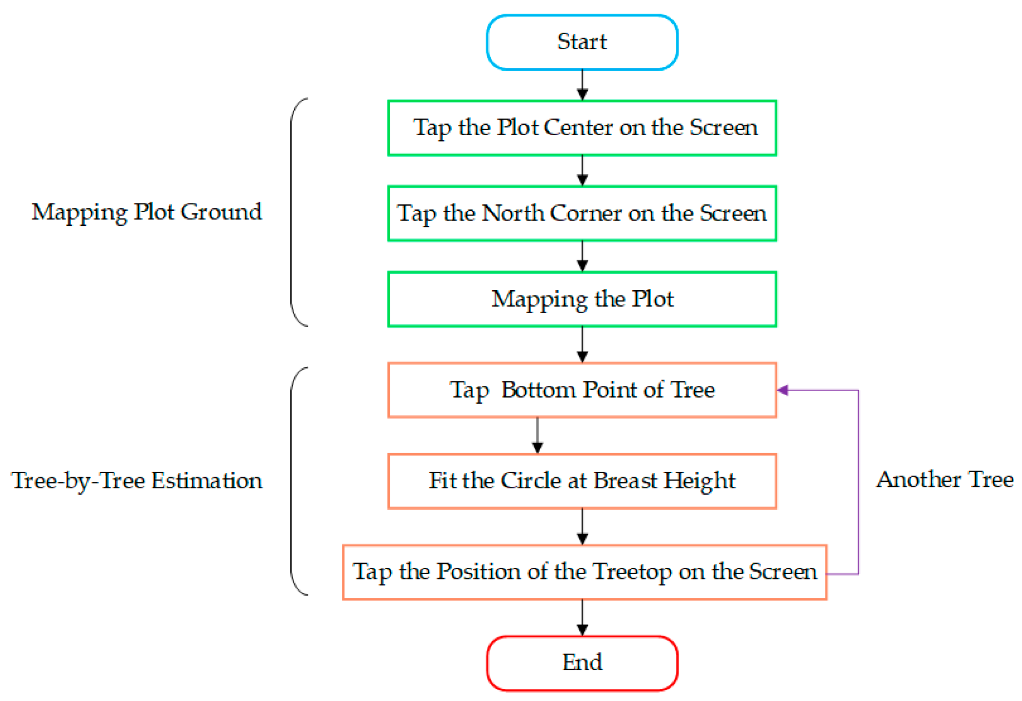
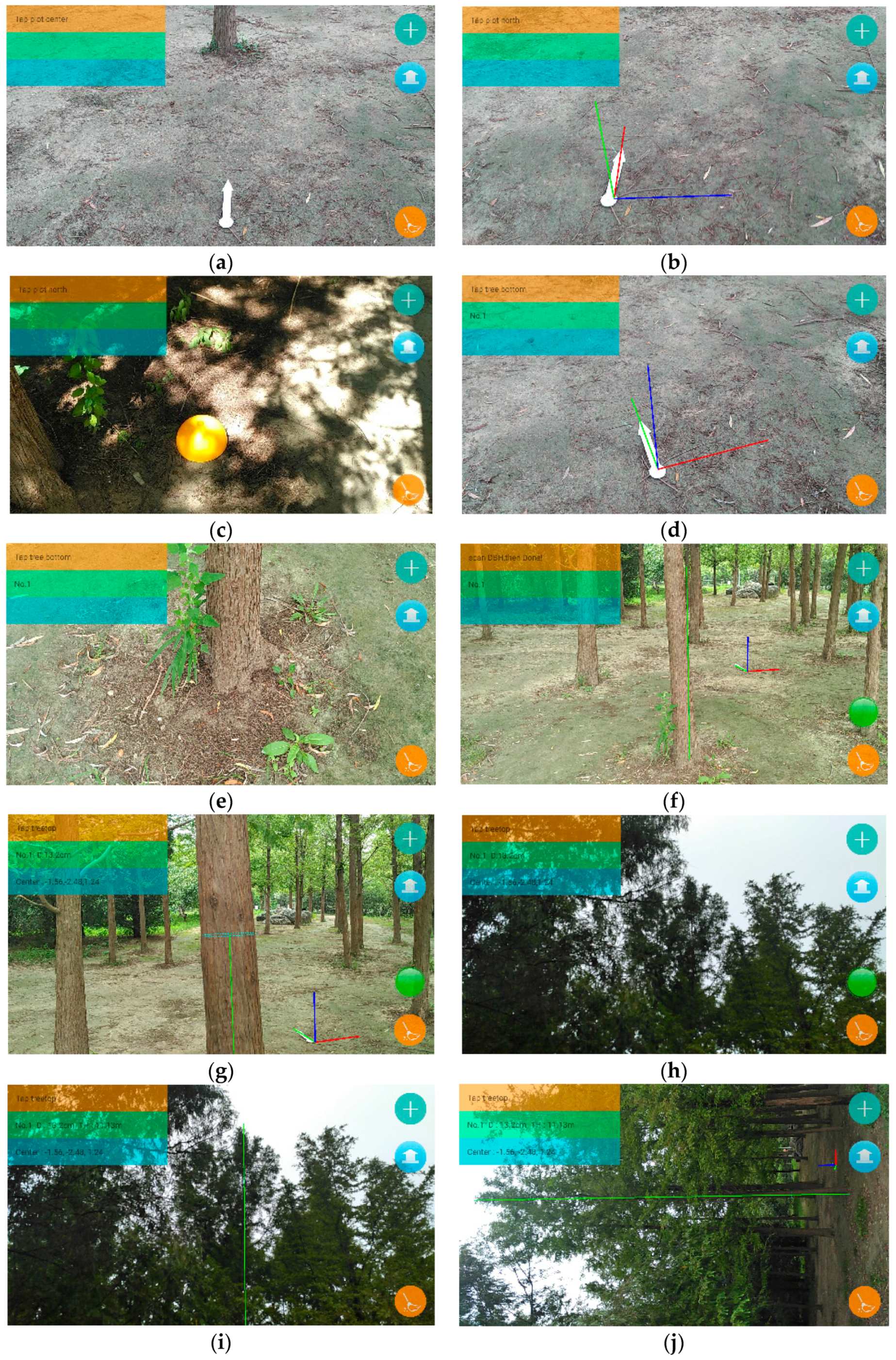
3.2.1. The System Workflow

An application was developed to enable the SLAM mobile phone to be used for forestry inventory. Figure 4 shows the workflow of our hardware and software system. The SLAM system uses an RGB-D camera and an inertial measurement unit (IMU) as inputs and produces RGB images, point clouds, poses, and time stamps. Our forest inventory system uses these data, and then interacts with the Android system to show the results on a screen or accept instructions from users. The forest inventory system includes mapping the plot ground and tree-by-tree estimation, as shown in Figure 5. The mapping process should provide a globally consistent map and the plot coordinate system for tree-by-tree estimation.

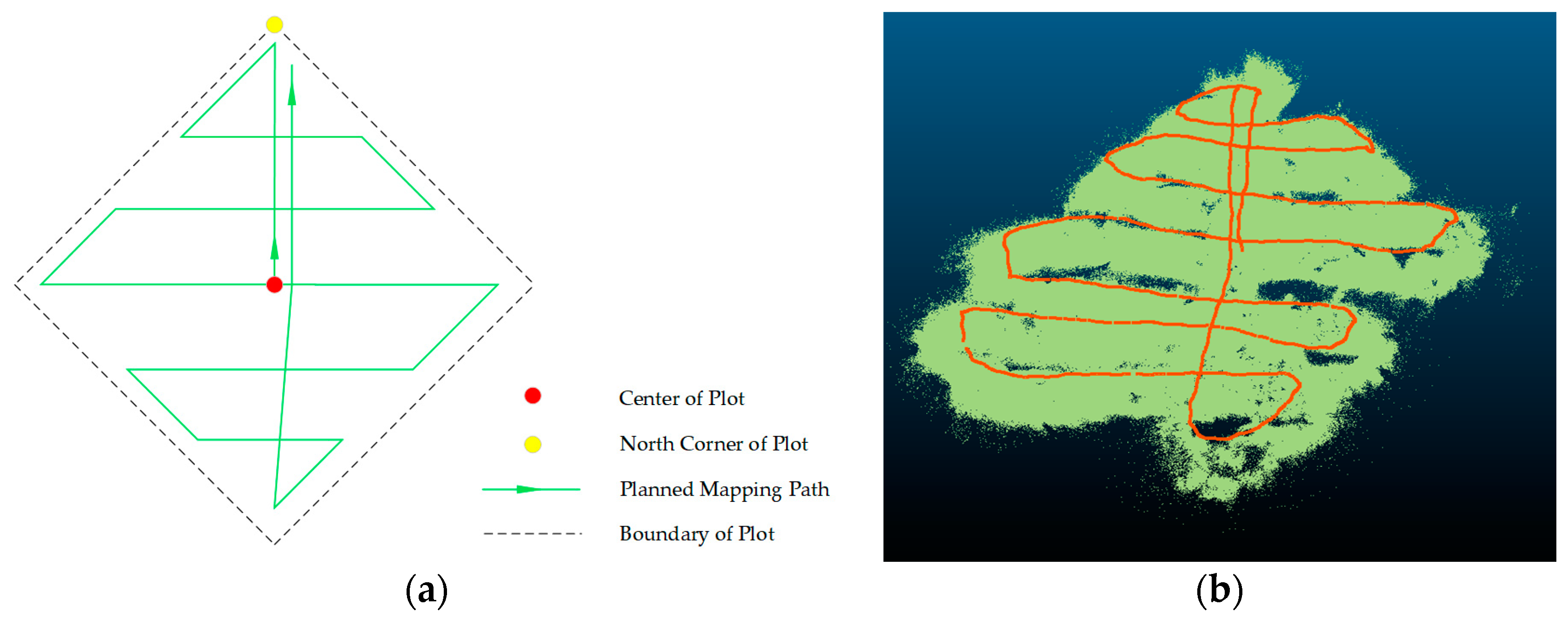
3.2.2. Mapping of the Plot Ground

The plot ground was mapped before observing the trees. That mapping was used to correct the poses of the mobile phone when observing the trees through loop-closure detection and pose graph nonlinear optimization. To obtain a globally consistent plot ground map, the scan path was designed as shown in Figure 6a. The plot center was used as the starting point of the mapping process towards the north of the plot, while the end was near to the north point. Figure 6b shows a typical instance of mapping path.

Building the Plot Coordinate System

Before measuring the tree attributes, we built a new coordinate system during the mapping process to describe the position of each tree in the plot. This coordinate system, known as the Plot Coordinate System (PCS), has the center of the plot as its origin, and the horizontal eastward/horizontal northward/vertical upward directions were defined as the x/y/z-axis directions. However, the mobile phone defined a coordinate system known as the Initial Coordinate System (ICS), in which the origin is the position of the device when it is initiated, the x-axis is towards the right side of the phone screen, and the y-axis is directed vertically upward, while the z-axis is towards the mobile phone screen. Conversion of the coordinate system was needed after the center and the north corner of the plot had been tapped on the screen during the mapping process, as shown in Figure 7a–c. The center of the plot was tapped at the beginning of the mapping process, and the north corner was tapped at the end of the mapping process. After that, the transformation matrix between the PCS and the ICS was obtained. Then, the PCS was transformed into the OpenGL coordinate system and displayed as shown in Figure 7d.

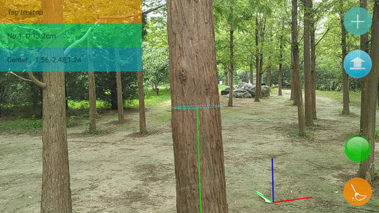
3.2.3. Estimation of the Stem Position, DBH, and Tree Height

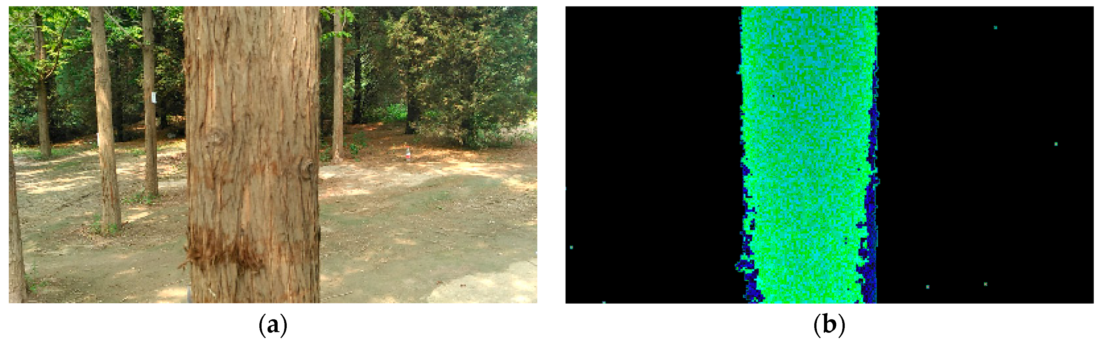
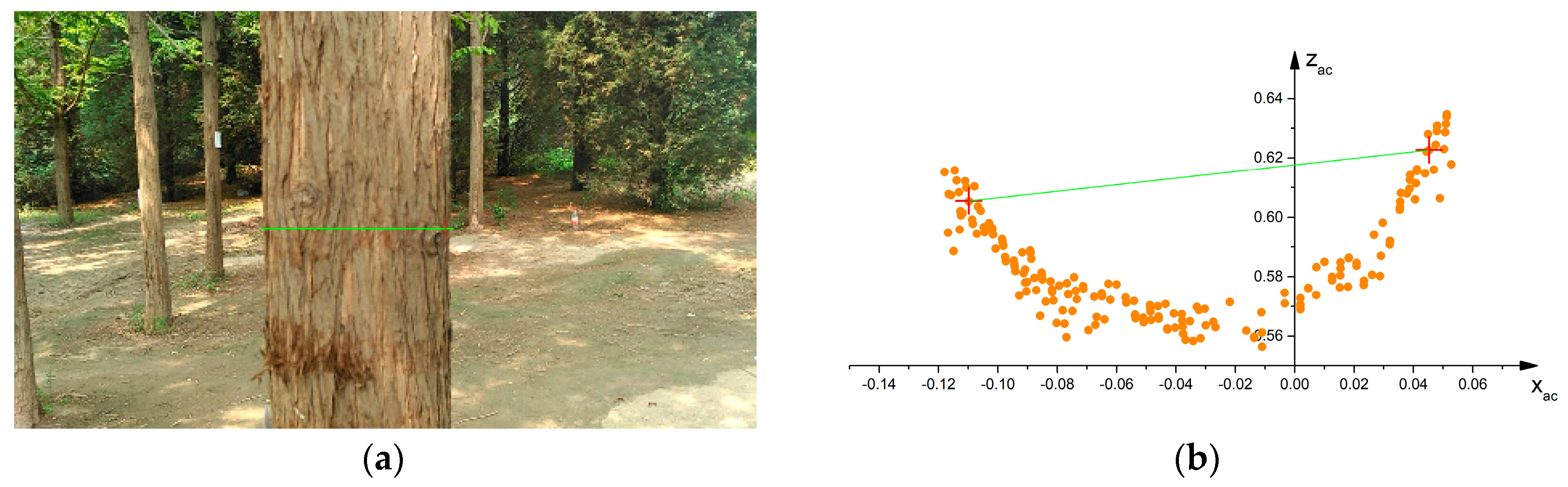
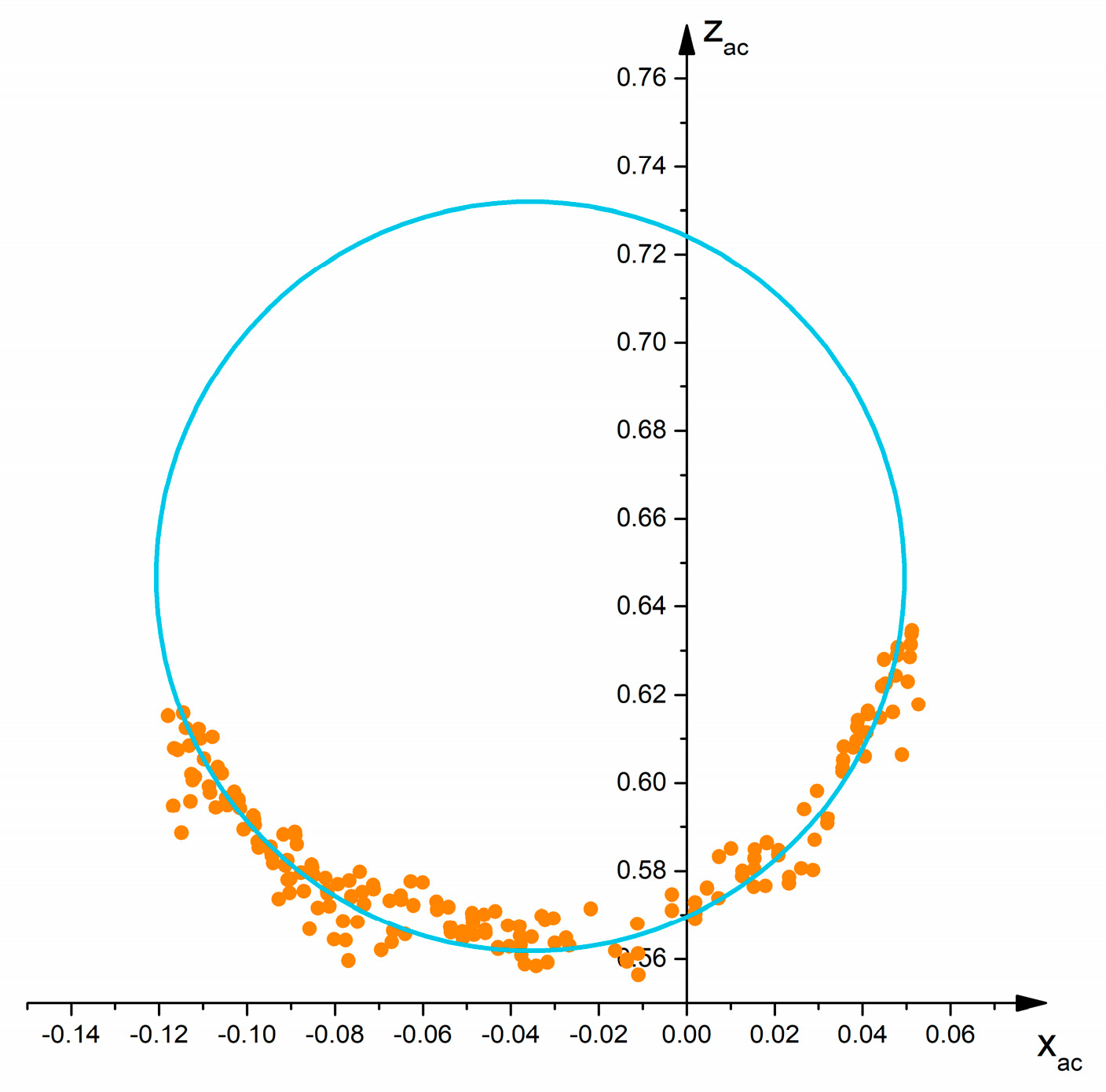
Estimation of the stem position and DBH

After mapping the plot ground, we were able to observe each tree individually. While observing a standing tree, a point near the bottom of the tree was acquired to determine the breast height and the approximate stem position (see Figure 7e,f). After the bottom point had been taken, the breast height was displayed on the screen as shown in Figure 7f. Then, the position of the stem center and DBH were calculated using the current camera pose and the point cloud (Figure 8).
For convenience of operation, an auxiliary coordinate system (Auxiliary Camera Coordinate System, ACCS) was established with a similar origin to that of the camera coordinate system (CCS), as the y-axis direction was same as the y-axis direction of the PCS (vertically upward), and the z-axis was in the plane formed by the new y-axis and the z-axis of the CCS. The point cloud data were constructed and transformed into the ACCS. The points belonging to the tree were filtered according to the bottom point ( x a c _ b o t t o m ). Figure 9 shows the scatter plot of these points on the plane O a c x a c z a c , while the filter conditions were set to
  { x a c _ b o t t o m 1 < x a c < x a c _ b o t t o m + 1 z a c _ b o t t o m 1 < z a c < z a c _ b o t t o m + 1 y a c _ b o t t o m 1.25 < y a c < y a c _ b o t t o m + 1.25  
The marginal distribution of all filtered points in the x-axis direction was approximately uniformly distributed (Figure 10). When the mean ( μ x ) and variance ( σ x ) of the points were calculated, the range of the stem was ( μ x 3 σ x ,   μ x + 3 σ x ) in the x-axis direction. RANSAC (Random Sample Consensus) was used to improve the robustness of the interval in this process (Figure 11).
The two edges of the stem were underestimated due to the assumption of uniform distribution. The stem edges were adjusted by linear fitting the points near to the stem edges, and the point on each fitted line that was farthest from the previous estimation interval was used as the boundary point (Figure 12); RANSAC was used in the process too.
The TOF camera uses the principle of perspective projection to obtain images. So, when the stem edge points were defined as T 1 and T 2 , both were the tangent points of the stem circle and the lines T 1 O a c and T 2 O a c . The stem circle needed to meet the following conditions: ① Line T 1 O a c and T 2 O a c had to be the tangents of the circle and points T 1 , T 2 had to be the tangent points; and ② The points between point T 1 and point T 1 had to be in the circle. Condition ① could be expressed as the cost functions:
  r = w · [ z T 1 ( z c z T 1 ) + x T 1 ( x c x T 1 ) ]  
  r = w · [ z T 2 ( z c z T 2 ) + x T 2 ( x c x T 2 ) ]  
  r = w · [ d 2 / 4   ( x c x T 1 ) 2   ( z c z T 1 ) 2 ]  
r = w · [ d 2 / 4   ( x c x T 2 ) 2   ( z c z T 2 ) 2 ] .
Here,   r is the residual to be optimized; w is the weight of the cost function; X T 1 = ( x T 1 , z T 1 ) and X T 2 = ( x T 2 , z T 2 ) are the coordinates of points T 1 and T 2 in the plane O a c x a c z a c ; X c = ( x c , z c ) is the stem center coordinate; and d is the DBH of the tree. Each point in Condition ② can be constructed as the cost function
r = d 2 4 ( x c x i ) 2   ( z c z i ) 2 .
Here, X i = ( x i , z i ) is one of the points between points T 1 and T 2 in the circle. Because condition ① is more important for the circle fitting than condition ②, the weight w should have a large value. In this paper, it was determined according to Condition ②; if the number of points in the optimization process was defined as N in condition ②, the weight w was equal to N/4. After the cost functions had been constructed, the Levenberg Marquardt algorithm was used to fit the stem circle. To increase the robustness of the optimization result, RANSAC was used in the fitting process. Figure 13 shows the fitting circle. Then, the stem position coordinate was converted into the PCS and projected into the OpenGL coordinate system, so the result could be viewed from the display (Figure 7g).

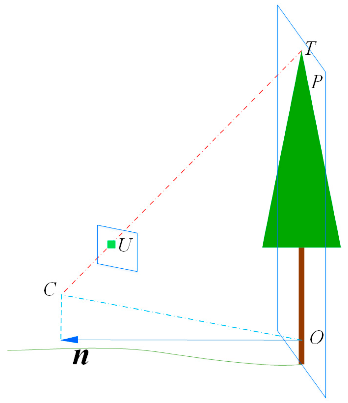
Estimation of the tree height

To estimate the height of the tree, the device was kept at a position where the treetop could be observed simultaneously (Figure 7h). After tapping the treetop position on the screen, the tree height was calculated in real time. As the treetop was on the connection line between the optical center of the camera and the tapped pixel (Figure 14), the coordinates of the treetop point were expressed as
x p _ t o p = t p _ c + k R p _ c K 1 u .
Here, x p _ t o p = ( x p _ t o p , y p _ t o p , z p _ t o p ) T is the coordinate of the treetop point in the PCS; t p _ c is the translation vector of the camera in the PCS; R p _ c is the rotation matrix of the camera in the PCS; K is the intrinsic matrix of the camera; u = ( u , v , 1 ) T is the coordinate of the treetop pixel in the pixel coordinate system; k is an unknown factor. However, additional conditions were needed to determine k. If the standing tree was assumed to be vertical, the treetop would be on the vertical line passing through the center of the stem, but since a natural stem is not exactly vertical and the tapped treetop pixel showed deviation, the two lines were difficult to intersect or even impossible to intersect. To solve this problem, we assumed that the treetop was on the plane of the stem center, whose normal vector is denoted by
n = [ 1 0 0 0 0 0 0 0 1 ] ( t p _ c x p _ c e n t e r ) .
Here, x p _ c e n t e r = ( x p _ c e n t e r , y p _ c e n t e r , z p _ c e n t e r ) T is the central coordinate of the stem. In this way, the treetop coordinate satisfied
( x p _ t o p x p _ c e n t e r ) · n = 0 .
Then, after being calculated from (11) and (13), the treetop coordinate x p _ t o p was
x p _ t o p = t p _ c + ( x p _ c e n t e r t p _ c ) · n ( R p _ c K 1 u ) · n · ( R p _ c K 1 u ) .
Naturally, the tree height h equaled
h = y p _ t o p y p _ c e n t e r + 1.3 .
As shown in Figure 7i,j, the treetop point x p _ t o p was projected into the OpenGL coordinate system and displayed on the screen.

3.2.4. Evaluation of the Accuracy of the Stem Position, DBH and Tree Height Measurements

Stem position references were determined by total station (Leica Flexline TS06plus Total Station) measurement data, and DBH measurements. When measuring the position of a tree, the total station was installed in the center of the plot. The angle between the stem and north and the horizontal distance from the plot center to the trunk were measured by the total station and recorded. The true distance true position of the stem was calculated from the distance and angle, and the center point of the stem was needed for true position calculation. The stem position errors were described by a mean vector μ and a two-dimensional covariance matrix Σ , as follows:
  μ = [ μ x μ y ] = [ i = 1 n ( x i x i r ) n i = 1 n ( y i y i r ) n ]  
  Σ = i = 1 n [ x i x i r μ x y i y i r μ y ] [ x i x i r μ x y i y i r μ y ] T  
Here, ( x i , y i ) is the ith position measurement. ( x i r , y i r )   is the ith reference, and n is the number of estimations. The direction of the eigenvector corresponding to the largest eigenvalue of the covariance matrix is the direction with the greatest variability. The standard deviation of this direction is equal to the square root of the largest eigenvalue, which can describe the variability of the trunk position, and can be expressed as
σ m a x = m a x ( e i g e n v a l u e s ( Σ ) ) .
The references of the DBH were measured using a taper and the references of the tree height were measured using a total station. The accuracy of the DBH and tree height measurements were evaluated using BIAS, root mean square error (RMSE), relative BIAS, and relative RMSE, as defined in the following equations:
  BIAS = i = 1 n ( x i x i r ) n  
  relBIAS = i = 1 n ( x i / x i r 1 ) n × 100 %  
  RMSE = i = 1 n ( x i x i r ) 2 n  
  relRMSE = i = 1 n ( x i / x i r 1 ) 2 n × 100 %  
Here, x i is the ith measurement. x i r is the ith reference. n is the number of estimations. RMSE is also a way of describing the accuracy of the tree position by computing the values in the x-axis and y-axis directions, respectively.

4. Results

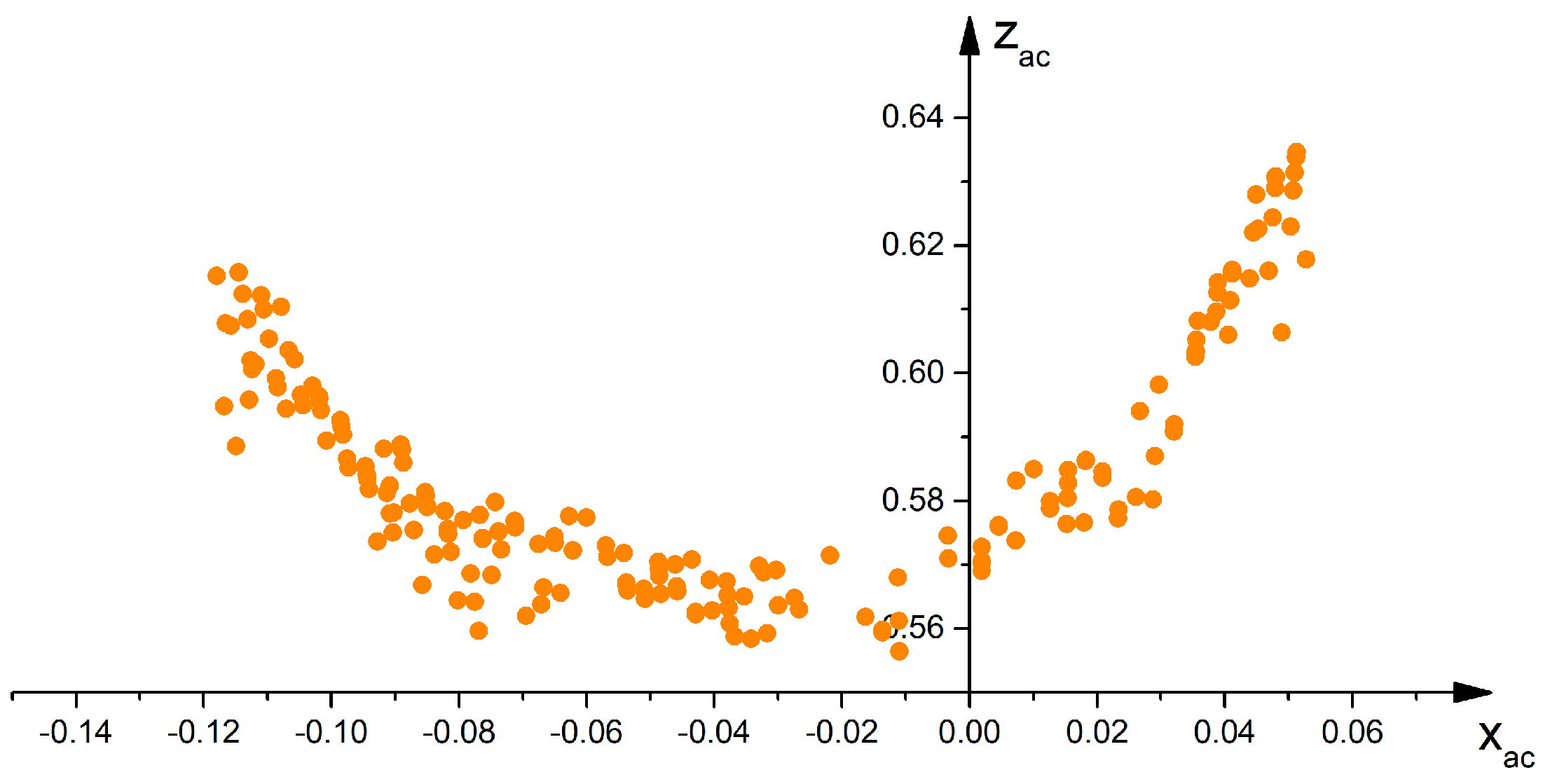
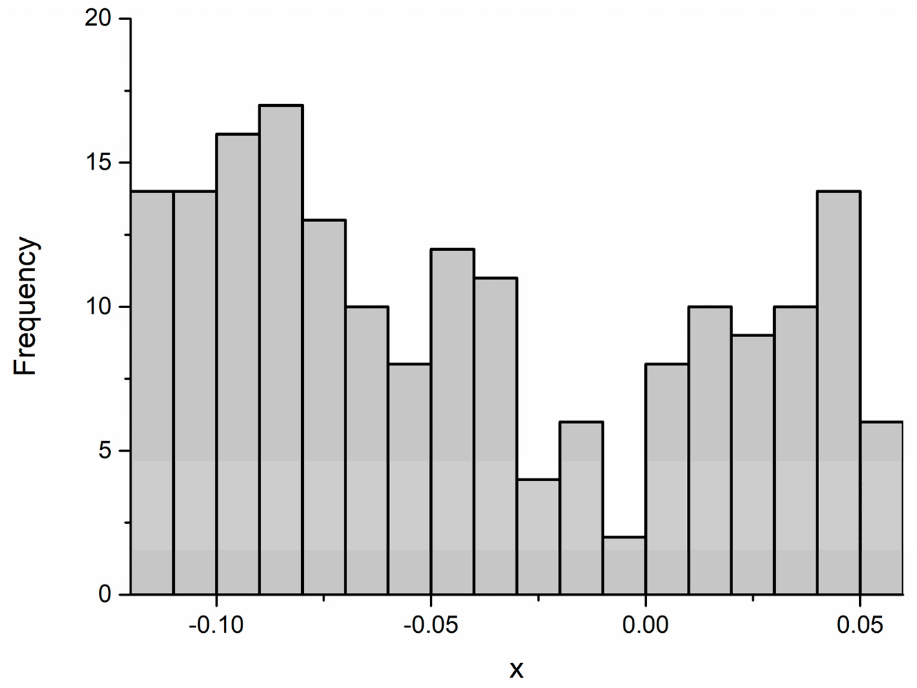
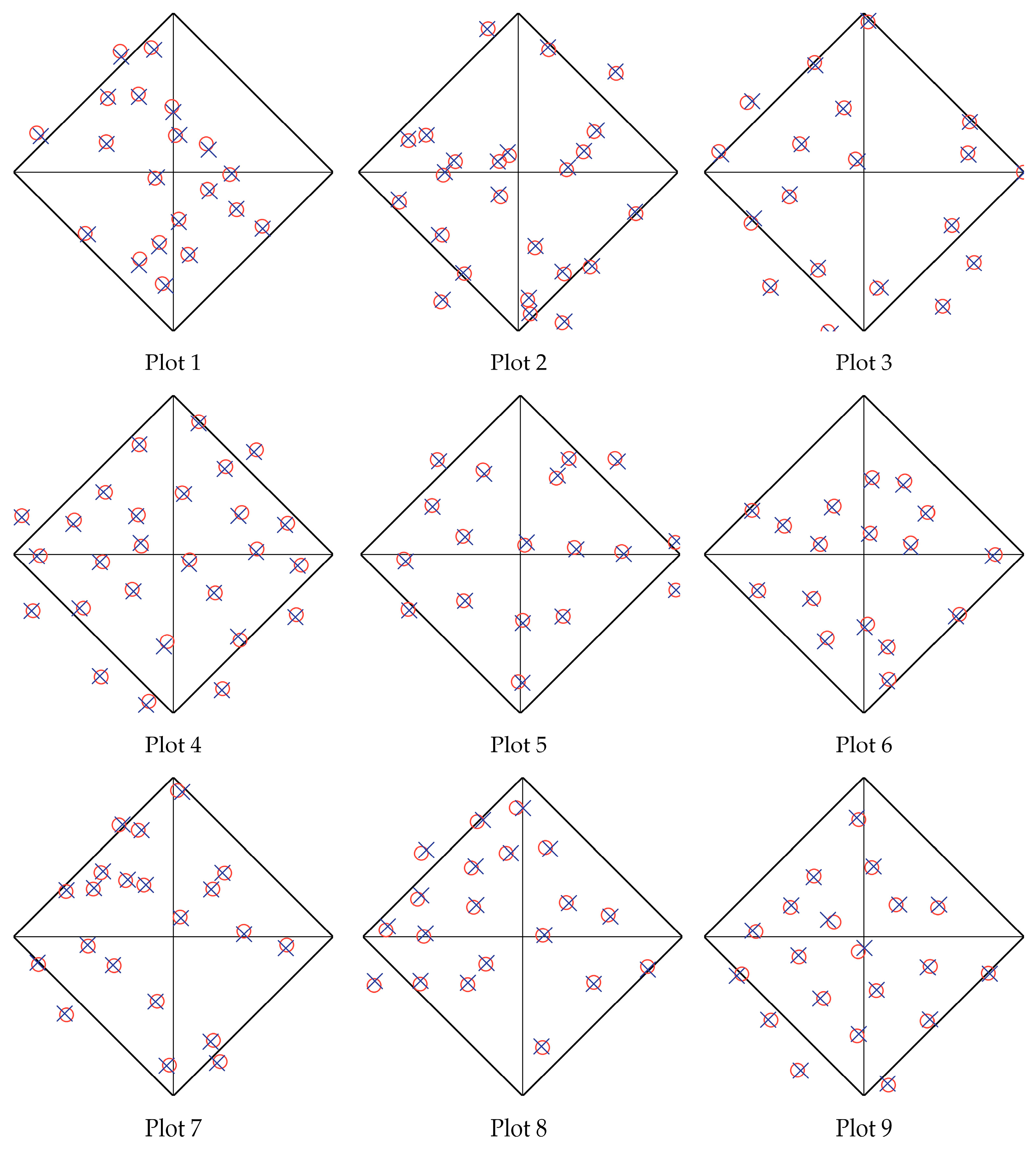
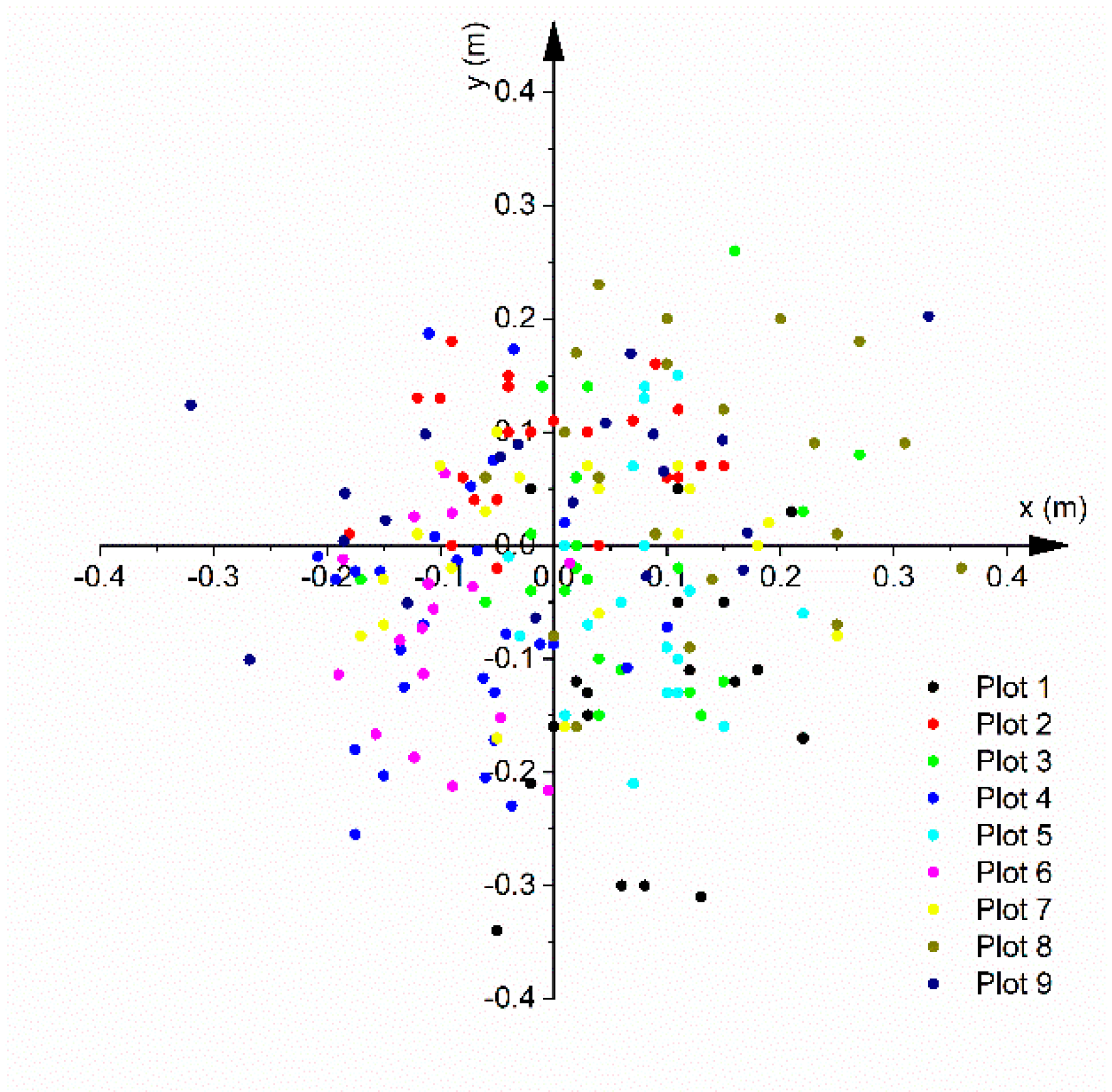
4.1. Evaluation of Tree Position

The estimated stem positions are given in Figure 15. The accuracy of the stem position was checked with a total station instrument. Our results showed that the range of the average error was approximately −0.12 m to 0.13 m in both the x-axis and y-axis directions, as shown in Table 2. In addition, no significant correlation (approximately −0.08 to 0.35) was found between the errors in the x-axis and y-axis directions, so the standard deviations of the maximum variability direction (0.09~0.16 m) were close to the x-axis (0.05~0.16 m) and y-axis (0.05~0.13 m). The RMSEs in the x-axis (0.09~0.17 m) and y-axis (0.07~0.17 m) directions were also close. As shown in Figure 16, although the tree position estimated for each plot had systematic errors, there was a weak error overall. This shows that the systematic errors were random in different sample plots. The overall standard deviation in the maximum variability direction was small (0.10 m) in all plots.

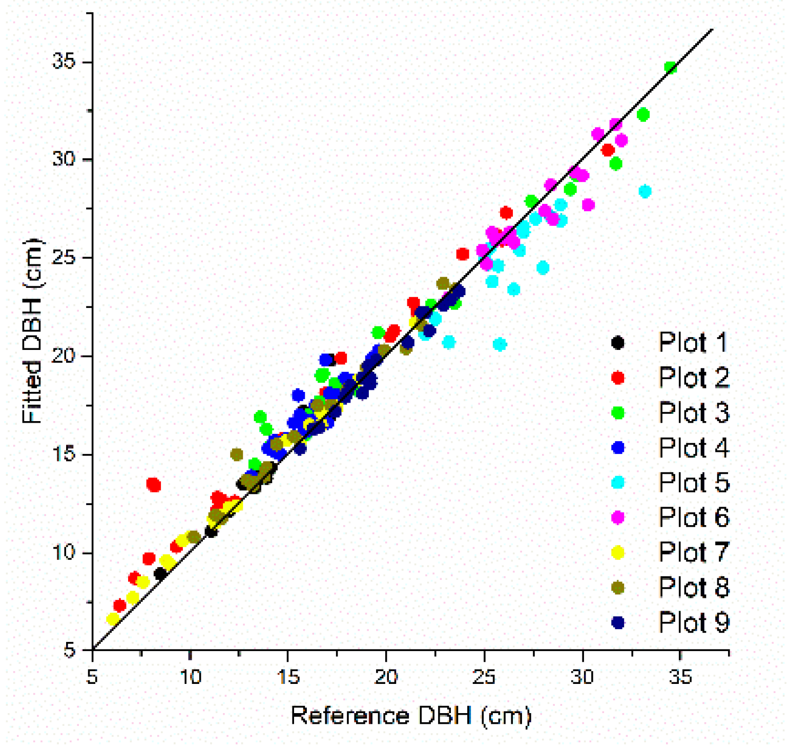
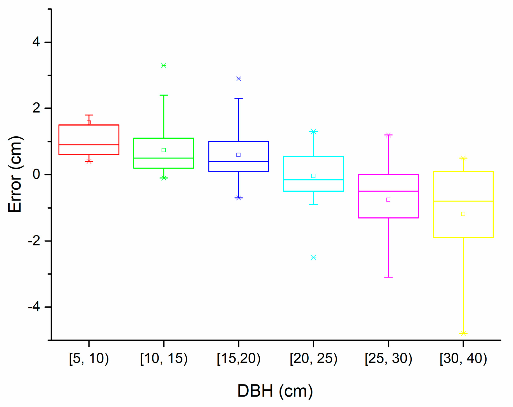
4.2. Evaluation of DBH

The DBH values measured by the smartphone with RGB-D sensor were compared with field data that were measured using diameter tape. Our results showed that our estimated values of DBH were similar to the reference data obtained in the field (Figure 17). Table 3 describes the statistical results of the DBHs in different plots. A 1.26 cm (6.39%) RMSE and a 0.33 cm (1.78%) BIAS is shown for all plots. Figure 18 shows that for smaller DBH values, our estimated results were larger than the reference value, while the case was reversed for larger DBH values. It can also be seen from the figure that the dispersion of observations was relatively stable.

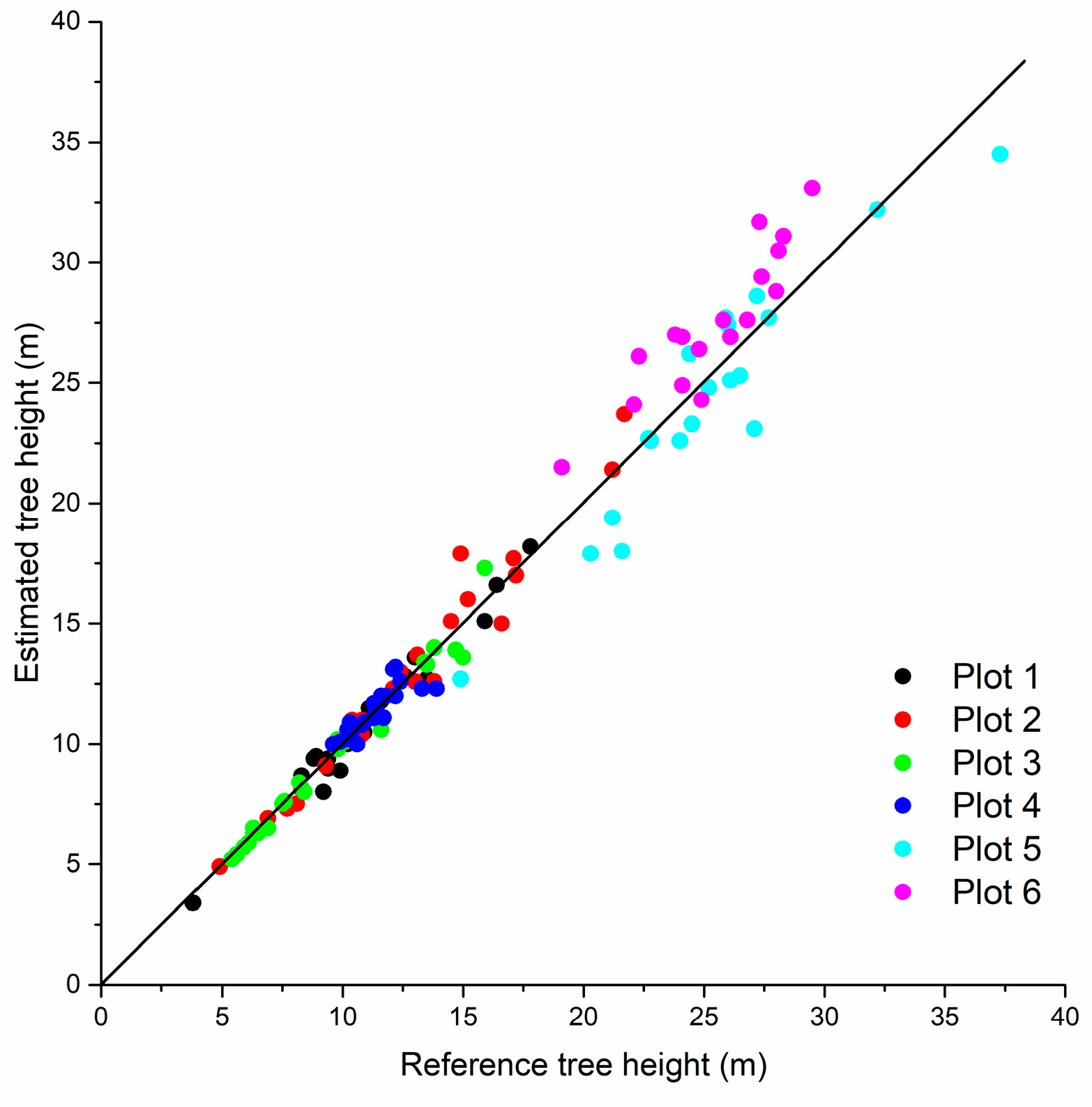
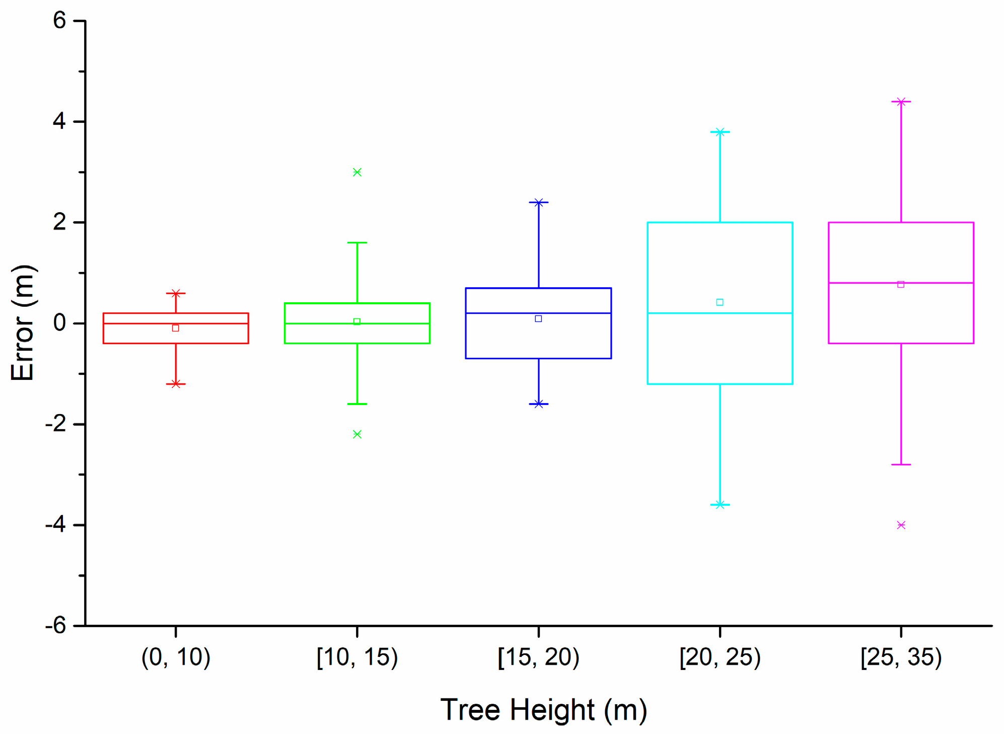
4.3. Evaluation of Tree Height

Our estimated results of the tree heights were similar to the reference field data measured by total stations (Figure 19). The statistical results are summarized in Table 4. It is shown that the estimations generally had smaller BIAS (0.07 m, 0.54%) and RMSE (0.55 m, 3.71%) values, except plot 5 and plot 6. The dispersion of observed values increased as the tree height increased, as shown in Figure 20.

5. Discussion

SLAM technology provides a solution for positioning without GNSS signals in places like forests. In this study, we measured the positions, DBHs, and heights of trees in real-time using the poses and dense point cloud data provided by a phone with RGB-D SLAM.
The tree positions were obtained from the device pose and a circle was fitted to the points around the breast height of each tree trunk. The drift of the phone pose mainly affected the accuracy of the tree positions. In this paper, a global consistency map of the plot ground was pre-built; it can be used to reduce the drift by loop-closure detection and pose graph nonlinear optimization. Our result showed an error of approximately −0.12 to 0.13 m on both the x-axis and the y-axis and a 0.1~0.16 m standard deviation in the maximum variability direction; the RMSEs were 0.09~0.17 m and 0.07~0.17 m in the x-axis and the y-axis, respectively. Many studies have examined the extraction of tree positions, but few of them given results. Reference [22] used an unmanned ground vehicle with 3D LiDAR and graph-SLAM to scan the study area, and the error for the relative distance estimation between trees was 0.0476 m. Reference [25] used a Small-Footprint Mobile LiDAR to scan the study area, resulting in RMSEs of the motion trajectories in the two different areas of 0.32 m and 0.29 m, respectively, but no detail of the positional accuracy of the trees was provided. However, those studies were conducted over a relatively larger study areas than ours; therefore, our method of using the mobile phone with RGB-D SLAM needs to be tested for accuracy over large areas. Reference [33] used Tango-based point clouds to extract tree positions offline, showing an RMSE value of 0.105 m for distances from the central point in the better scanning pattern, which is similar to our results.
We attempted to attain the DBH values from point clouds. The method has been widely studied; Reference [34] extracted DBH values by fitting circles to the point cloud at breast height using three different algorithms (Lemen, Pratt and Taubin), and the results showed that the BIAS value was approximately −0.12 to 0.07 cm and the RMSE was 1.47~2.43 cm in single scan mode, while in merged scan mode, the BIAS was approximately −0.32 to 0 cm, and the RMSE was 0.66~1.21 cm. Similarly, reference [15] extracted DBH values by fitting the cylindrical and point cloud data from TLS that showed a BIAS value of approximately −0.18 to 0.76 cm and an RMSE value of 0.74~2.41 cm when using the single-scan method; however, the BIAS value was 0.11~0.77 cm and the RMSE was 0.90~1.90 cm when using the multi-single-scan method. Reference [35] extracted DBH values using the Hough transformation and the RANSAC algorithm; their results showed a BIAS value of approximately −0.6 to 1.3 cm and an RMSE value of 2.6~5.9 cm. Reference [33] obtained DBHs from Tango-based point clouds, and the RMSEs were in the range of 1.61~2.10 cm. This paper showed a 1.26 cm (6.39%) RMSE and a 0.33 cm (1.78%) BIAS. In our study, the point clouds for detecting DBH originated from a TOF camera instead of a LiDAR; therefore, our work increased the tangential and tangent point constraints by detecting the trunk boundaries and using the perspective projection principle of the TOF camera. This could be a possible reason why higher accuracies were obtained with a low-quality point cloud compared to LiDAR. In addition, the AR technology in this paper showed the fitted circle at breast height on the screen in real-time, making it possible for the observer to judge whether it needed to be re-fitted or not, thus artificially reducing the interference caused by noise points.
The method used to measure the height in this paper was similar to the traditional altimeter, which calculates the attribute by measuring the distance from the observation position to the tree and the inclinations of the tree bottom and treetop. The results showed a BIAS value of approximately –0.83 to 2.08 m and an RMSE value of 0.46~2.44 m. The result also showed that the measurement results had high precision when the tree was not higher than 20 m, as shown in Figure 20, although AR technology was used, which enabled the observer to determine whether the displayed treetop position was appropriate; otherwise, it was adjusted as needed. This may be influenced by occlusion and the subjective decisions of observers. Reference [36] evaluated a Laser-relascope, a classical traditional instrument; they reported a −0.016 m BIAS and a 0.190 m standard deviation. The limitation of the Laser-relascope is that it needs to be mounted on a fixed site, but our device did not need that. Reference [15] used the height difference between the ground level and highest point on the point cloud around the tree model, and obtained results with a BIAS value of approximately −1.30 to 1.50 m and an RMSE value of 1.36~4.29 m when using the single-scan method, while the BIAS value was approximately −0.34 to 2.11 m and the RMSE value was 2.04~6.53 m when using the multi-single-scan method. Reference [7] examined the consistency of the point cloud on the treetops when exclusively using TLS data compared to the previous method; the BIAS value was approximately −0.3 to 0.11 m and the RMSE value was 0.31~0.8 m. The point cloud at the treetop was difficult to obtain due to occlusion, so the estimates were not accurate. The device used in this article can acquire point clouds by using the TOF camera, but the measuring range is only 0.4~3.0 m, which makes it hard to get the point cloud at the treetop.
In the SLAM algorithm, corners or blobs are often used as visual feature points. A good feature should have localized accuracy (both in position and scale), repeatability, robustness, etc. However, it is difficult to find good corners or blobs, especially in forests with complex ground conditions, such as shrubs. The plot data used in this article were taken from human accessible areas with fewer shrubs on the ground. However, most forests will not meet these special conditions. In addition, the RGB camera needs to search for feature points in an environment with sufficient illumination, while the TOF camera is susceptible to strong illumination because it uses infrared light as its light source. Therefore, the device is only suitable for use under the canopies during the day.
Although the device is a possible option for forestry surveys, it still has some limitations. For example, (1) although the device can estimate forest inventory parameters in real-time, it is less efficient than TLS, MLS, or the previous uses of SLAM because of the need to access each tree individually; (2) the taller tree accuracy of our tree height estimates was compromised a little, perhaps due to drift; and (3) the tree position coordinates obtained by the device do not use the geodetic coordinate system, but rather, the plot coordinate system of the origin at the center of the plot. In addition, the device uses the manual selection method to locate the bottom of the tree.
Unfortunately, the Google Tango Project has been terminated, i.e., is longer being developed or supported. However, ARKit [37], a monocular SLAM system, was released by Apple. Google has also introduced a similar solution—ARCore [38]. These two technologies allow simultaneous localization and mapping for ordinary smartphones (without a TOF camera). Of course, due to the new features of these technologies, many aspects, such as how to get dense point clouds in real-time, still need to be investigated in the future.

6. Conclusions

This paper provided a solution to estimate tree position, DBH, and tree height under the canopy in real-time without GNSS signals using a mobile phone with RGB-D SLAM. The tree position and DBH were estimated by circle fitting the point cloud data. This paper added the tangent point constraints and the tangent constraints. The difference was that this article used the pose data provided by the SLAM system in real-time instead of using angles and distances to estimate tree height. The results showed that the tree height estimations were accurate, especially when the tree was not too tall. The experimental results also showed that this method can potentially be used to accurately estimate the tree position and DBH.
It is recommended that future research studies are carried out to test the device under complex forest conditions, such as in areas with more shrubs, better or poorer light, different tree species, and in different aged forests. Future studies should also focus on extracting other forest inventory attributes, such as stem curves and crown diameters.

Author Contributions

Methodology, Y.F. and Z.F.; Software, Y.F.; Data processing, A.M.; Compilation and formal analysis, A.M. and T.U.K.; Writing–original draft, Y.F.; Writing–review & editing, T.U.K. and C.S.; Proof reading, T.U.K. and S.S.

Funding

This work was supported by the National Natural Science Foundation of China (Grant number U1710123), the Medium-to-long-term project of young teachers’ scientific research in Beijing Forestry University (Grant number 2015ZCQ-LX-01) and the Beijing Municipal Natural Science Foundation (Grant number 6161001).

Acknowledgments

The authors wish to say thanks to E.M., S.C., W.M., Y.T., and Y.L. for help collecting data.

Conflicts of Interest

The authors declare no conflict of interest.

References

  1. Trumbore, S.; Brando, P.; Hartmann, H. Forest health and global change. Science 2015, 349, 814–818. [Google Scholar] [CrossRef] [PubMed]
  2. FAO (Food and Agriculture Organization of the United Nations). Global Forest Resources Assessment 2010; Main report, FAO Forest paper; FAO: Rome, Italiy, 2010; Volume 163. [Google Scholar]
  3. Tubiello, F.N.; Salvatore, M.; Ferrara, A.F.; House, J.; Federici, S.; Rossi, S.; Biancalani, R.; Condor Golec, R.D.; Jacobs, H.; Flammini, A.; et al. The contribution of agriculture, forestry and other land use activities to global warming, 1990–2012. Glob. Chang. Biol. 2015, 21, 2655–2660. [Google Scholar] [CrossRef] [PubMed] [Green Version]
  4. MacDicken, K.G. Global forest resources assessment 2015: What, why and how? For. Ecol. Manag. 2015, 352, 3–8. [Google Scholar] [CrossRef]
  5. Reutebuch, S.E.; Andersen, H.-E.; McGaughey, R.J. Light detection and ranging (LIDAR): An emerging tool for multiple resource inventory. J. For. 2005, 103, 286–292. [Google Scholar]
  6. Liang, X.; Kankare, V.; Hyyppä, J.; Wang, Y.; Kukko, A.; Haggrén, H.; Yu, X.; Kaartinen, H.; Jaakkola, A.; Guan, F.; et al. Terrestrial laser scanning in forest inventories. ISPRS J. Photogramm. Remote Sens. 2016, 115, 63–77. [Google Scholar] [CrossRef] [Green Version]
  7. Cabo, C.; Ordóñez, C.; López-Sánchez, C.A.; Armesto, J. Automatic dendrometry: Tree detection, tree height and diameter estimation using terrestrial laser scanning. Int. J. Appl. Earth Obs. Geoinf. 2018, 69, 164–174. [Google Scholar] [CrossRef]
  8. Barrett, F.; McRoberts, R.E.; Tomppo, E.; Cienciala, E.; Waser, L.T. A questionnaire-based review of the operational use of remotely sensed data by national forest inventories. Remote Sens. Environ. 2016, 174, 279–289. [Google Scholar] [CrossRef]
  9. Suciu, G.; Ciuciuc, R.; Pasat, A.; Scheianu, A. Remote Sensing for Forest Environment Preservation. In Proceedings of the 2017 World Conference on Information Systems and Technologies, Madeira, Portuga, 11–13 April 2017; pp. 211–220. [Google Scholar]
  10. Gougherty, A.V.; Keller, S.R.; Kruger, A.; Stylinski, C.D.; Elmore, A.J.; Fitzpatrick, M.C. Estimating tree phenology from high frequency tree movement data. Agric. For. Meteorol. 2018, 263, 217–224. [Google Scholar] [CrossRef]
  11. Alcarria, R.; Bordel, B.; Manso, M.Á.; Iturrioz, T.; Pérez, M. Analyzing UAV-based remote sensing and WSN support for data fusion. In Proceedings of the 2018 International Conference on Information Technology & Systems, Libertad City, Ecuador, 10–12 January 2018; pp. 756–766. [Google Scholar]
  12. Lim, K.; Treitz, P.; Wulder, M.; St-Onge, B.; Flood, M. LiDAR remote sensing of forest structure. Prog. Phys. Geogr. 2003, 27, 88–106. [Google Scholar] [CrossRef]
  13. Liang, X.; Litkey, P.; Hyyppa, J.; Kaartinen, H.; Vastaranta, M.; Holopainen, M. Automatic stem mapping using single-scan terrestrial laser scanning. IEEE Trans. Geosci. Remote Sens. 2012, 50, 661–670. [Google Scholar] [CrossRef]
  14. Béland, M.; Widlowski, J.-L.; Fournier, R.A.; Côté, J.-F.; Verstraete, M.M. Estimating leaf area distribution in savanna trees from terrestrial LiDAR measurements. Agric. For. Meteorol. 2011, 151, 1252–1266. [Google Scholar] [CrossRef]
  15. Liang, X.; Hyyppä, J. Automatic stem mapping by merging several terrestrial laser scans at the feature and decision levels. Sensors 2013, 13, 1614–1634. [Google Scholar] [CrossRef] [PubMed]
  16. Srinivasan, S.; Popescu, S.C.; Eriksson, M.; Sheridan, R.D.; Ku, N.-W. Terrestrial laser scanning as an effective tool to retrieve tree level height, crown width, and stem diameter. Remote Sens. 2015, 7, 1877–1896. [Google Scholar] [CrossRef]
  17. Liang, X.; Hyyppä, J.; Kukko, A.; Kaartinen, H.; Jaakkola, A.; Yu, X. The use of a mobile laser scanning system for mapping large forest plots. IEEE Geosci. Remote Sens. Lett. 2014, 11, 1504–1508. [Google Scholar] [CrossRef]
  18. Lin, Y.; Hyyppa, J. Multiecho-recording mobile laser scanning for enhancing individual tree crown reconstruction. IEEE Trans. Geosci. Remote Sens. 2012, 50, 4323–4332. [Google Scholar] [CrossRef]
  19. Ryding, J.; Williams, E.; Smith, M.J.; Eichhorn, M.P. Assessing handheld mobile laser scanners for forest surveys. Remote Sens. 2015, 7, 1095–1111. [Google Scholar] [CrossRef]
  20. Bauwens, S.; Bartholomeus, H.; Calders, K.; Lejeune, P. Forest inventory with terrestrial LiDAR: A comparison of static and hand-held mobile laser scanning. Forests 2016, 7, 127. [Google Scholar] [CrossRef]
  21. Forsman, M.; Holmgren, J.; Olofsson, K. Tree stem diameter estimation from mobile laser scanning using line-wise intensity-based clustering. Forests 2016, 7, 206. [Google Scholar] [CrossRef]
  22. Pierzchała, M.; Giguère, P.; Astrup, R. Mapping forests using an unmanned ground vehicle with 3D LiDAR and graph-SLAM. Comput. Electron. Agric. 2018, 145, 217–225. [Google Scholar] [CrossRef]
  23. Durrant-Whyte, H.; Bailey, T. Simultaneous localization and mapping: Part, I. IEEE Robot. Autom. Mag. 2006, 13, 99–110. [Google Scholar] [CrossRef]
  24. Bailey, T.; Durrant-Whyte, H. Simultaneous localization and mapping (SLAM): Part II. IEEE Robot. Autom. Mag. 2006, 13, 108–117. [Google Scholar] [CrossRef]
  25. Tang, J.; Chen, Y.; Kukko, A.; Kaartinen, H.; Jaakkola, A.; Khoramshahi, E.; Hakala, T.; Hyyppä, J.; Holopainen, M.; Hyyppä, H. SLAM-aided stem mapping for forest inventory with small-footprint mobile LiDAR. Forests 2015, 6, 4588–4606. [Google Scholar] [CrossRef]
  26. Holmgren, J.; Tulldahl, H.; Nordlöf, J.; Nyström, M.; Olofsson, K.; Rydell, J.; Willén, E. Estimation of tree position and stem diameter using simultaneous localization and mapping with data from a backpack-mounted laser scanner. Int. Arch. Photogramm. Remote Sens. Spat. Inf. Sci. 2017, 42, 59–63. [Google Scholar] [CrossRef]
  27. Kukko, A.; Kaijaluoto, R.; Kaartinen, H.; Lehtola, V.V.; Jaakkola, A.; Hyyppä, J. Graph SLAM correction for single scanner MLS forest data under boreal forest canopy. ISPRS J. Photogramm. Remote Sens. 2017, 132, 199–209. [Google Scholar] [CrossRef]
  28. Foix, S.; Alenya, G.; Torras, C. Lock-in time-of-flight (ToF) cameras: A survey. IEEE Sens. J. 2011, 11, 1917–1926. [Google Scholar] [CrossRef] [Green Version]
  29. Aijaz, M.; Sharma, A. Google Project Tango. In Proceedings of the 2016 International Conference on Advanced Computing, Moradabad, India, 22–23 January 2016. [Google Scholar]
  30. Mur-Artal, R.; Tardós, J.D. ORB-SLAM2: An Open-Source SLAM System for Monocular, Stereo, and RGB-D Cameras. IEEE Trans. Robot. 2017, 33, 1255–1262. [Google Scholar] [CrossRef] [Green Version]
  31. Lenovo Phab 2 Pro. Available online: http://www3.lenovo.com/us/en/virtual-reality-and-smart-devices/augmented-reality/-phab-2-pro/Lenovo-Phab-2-Pro/p/WMD00000220/ (accessed on 22 October 2018).
  32. Hyyppä, J.; Virtanen, J.-P.; Jaakkola, A.; Yu, X.; Hyyppä, H.; Liang, X. Feasibility of Google Tango and Kinect for crowdsourcing forestry information. Forests 2017, 9, 6. [Google Scholar] [CrossRef]
  33. Tomaštík, J.; Saloň, Š.; Tunák, D.; Chudý, F.; Kardoš, M. Tango in forests–An initial experience of the use of the new Google technology in connection with forest inventory tasks. Comput. Electron. Agric. 2017, 141, 109–117. [Google Scholar] [CrossRef]
  34. Pueschel, P.; Newnham, G.; Rock, G.; Udelhoven, T.; Werner, W.; Hill, J. The influence of scan mode and circle fitting on tree stem detection, stem diameter and volume extraction from terrestrial laser scans. ISPRS J. Photogramm. Remote Sens. 2013, 77, 44–56. [Google Scholar] [CrossRef]
  35. Olofsson, K.; Holmgren, J.; Olsson, H. Tree stem and height measurements using terrestrial laser scanning and the RANSAC algorithm. Remote Sens. 2014, 6, 4323–4344. [Google Scholar] [CrossRef]
  36. Kalliovirta, J.; Laasasenaho, J.; Kangas, A. Evaluation of the laser-relascope. For. Ecol. Manag. 2005, 204, 181–194. [Google Scholar] [CrossRef]
  37. Buerli, M.; Misslinger, S. Introducing ARKit-Augmented Reality for iOS. In Proceedings of the 2017 Apple Worldwide Developers Conference, San Jose, CA, USA, 5–9 June 2017; pp. 1–187. [Google Scholar]
  38. ARCore. Available online: https://developers.google.com/ar/ (accessed on 22 October 2018).
Figure 1. The simultaneous localization and mapping (SLAM) problem. Here, x k is the state vector describing the pose of the mobile platform at time k; u k is the motion vector describing the movement of the platform from time k − 1 to time k; m j is the vector describing the position of the jth landmark.
Remotesensing 10 01845 g001
Figure 2. Structure of a smart phone (Lenovo Phab 2 Pro) with RGB-D SLAM.
Remotesensing 10 01845 g002
Figure 3. Location of study area.
Remotesensing 10 01845 g003
Figure 4. The workflow of our system.
Remotesensing 10 01845 g004
Figure 5. The workflow of the forest inventory system for data acquirement.
Remotesensing 10 01845 g005
Figure 6. The mapping path of plot ground. (a) Pre-survey designed scan path map for collecting data with mobile phone; (b) Post-survey data collection, and actual path map.
Remotesensing 10 01845 g006
Figure 7. Different states of the SLAM device during the observation process. (a) Waiting to tap the plot center on the screen; (b) waiting to move towards the north corner of the plot; (c) waiting to tap the north corner on the screen; (d) completion of the PCS building; (e) waiting to tap a bottom point of a tree; (f) waiting to scan the breast height section of the tree; (g) completion of fitting the circle at breast height; (h) waiting to tap the position of the treetop on the screen; (i) completion of the estimation of the tree height; (j) finished estimating the attributes of the tree.
Remotesensing 10 01845 g007
Figure 8. The RGB image and depth image used to calculate the stem position and DBH: (a) the RGB image; (b) the Depth image.
Remotesensing 10 01845 g008
Figure 9. The scatter plot of all filtered points on the plane O a c x a c z a c .
Remotesensing 10 01845 g009
Figure 10. The edge distribution of all filtered points in the x-axis direction.
Remotesensing 10 01845 g010
Figure 11. The stem boundary detection result by a uniform distribution: (a) the boundaries in the RGB image; (b) the boundaries on the plane O a c x a c z a c .
Remotesensing 10 01845 g011
Figure 12. The stem boundary detection result after linear fitting: (a) The boundaries in the RGB image; (b) The boundaries on the plane O a c x a c z a c .
Remotesensing 10 01845 g012
Figure 13. The fitted stem circle at breast height.
Remotesensing 10 01845 g013
Figure 14. The geometric relationship between the points in the tree height solution. O is the center of the stem at breast height; C is the optical center of the camera; T is the treetop; U is the treetop pixel on the image; n is the horizontal component vector of the O C vector; and P is the plane whose normal vector is n and on which O is a point.
Remotesensing 10 01845 g014
Figure 15. Estimated and reference stem positions: the red circles indicate the stem references; the blue crosses indicate the estimations.
Remotesensing 10 01845 g015
Figure 16. The position errors of all trees in the plots.
Remotesensing 10 01845 g016
Figure 17. Scatter plot of estimated DBH values.
Remotesensing 10 01845 g017
Figure 18. The errors of DBH observations for different DBH values.
Remotesensing 10 01845 g018
Figure 19. Scatter plot of estimated tree heights.
Remotesensing 10 01845 g019
Figure 20. The errors in the tree height observations for different tree heights.
Remotesensing 10 01845 g020
Table 1. Summary statistics of plot attributes.
PlotTree NumberDominant SpeciesDBH (cm)Tree Height (m)
MeanSDMinMaxMeanSDMinMax
120Metasequoia glyptostroboides14.12.28.517.511.13.13.817.8
226Ulmus spp.16.36.76.431.312.24.34.921.7
322Fraxinus chinensis & Ulmus spp.20.76.912.434.59.53.45.415.9
428Ginkgo biloba16.51.613.119.611.31.09.613.9
519Populus spp.26.12.322.030.225.14.514.937.3
617Populus spp.27.82.623.232.025.42.619.129.5
721Styphnolobium japonicum12.94.26.121.511.73.14.618.1
820Fraxinus chinensis16.14.010.223.510.83.71.216.4
920Ginkgo biloba19.62.415.623.712.81.810.417.5
Table 2. Accuracy of the stem position estimations using the SLAM smartphone.
Plot μ x
(m)
μ y
(m)
σ x
(m)
σ y
(m)
ρ x y σ m a x
(m)
RMSE x   RMSE y  
(m)(m)
10.08−0.120.080.130.200.130.110.17
20.000.080.090.050.090.090.090.10
30.05−0.010.090.100.120.100.110.10
4−0.08−0.060.070.110.050.100.110.12
50.08−0.040.060.10−0.040.100.100.11
6−0.10−0.080.050.08−0.080.080.120.12
70.00−0.010.120.070.120.120.120.07
80.130.060.110.110.010.110.170.13
9−0.010.050.160.080.350.160.160.09
Total0.01−0.010.100.090.100.100.120.12
ρ x y means correlation coefficient.
Table 3. Accuracy of the DBH estimations using the SLAM smartphone.
PlotRMSE (cm)relRMSE (%)BIAS (cm)relBIAS (%)
10.735.21%0.412.91%
21.8011.09%1.267.73%
31.507.27%0.753.63%
41.056.40%0.824.99%
52.228.39%−1.64−6.21%
60.893.19%−0.32−1.16%
70.513.97%0.403.06%
80.794.93%0.493.04%
90.391.99%−0.15−0.74%
Total1.266.39%0.331.78%
Table 4. Accuracy of the tree height estimations using the SLAM smartphone.
PlotRMSE (m)relRMSE (%)BIAS (m)relBIAS (%)
10.544.91%−0.08−0.72%
20.907.35%0.121.01%
30.545.70%−0.13−1.34%
40.564.94%0.050.44%
51.887.47%−0.83−3.31%
62.449.58%2.088.18%
70.766.53%0.413.50%
80.464.22%−0.18−1.67%
90.755.90%−0.16−1.25%
Total1.117.43%0.151.08%

