Sparse Cost Volume for Efficient Stereo Matching

Abstract

Stereo matching has been solved as a supervised learning task with convolutional neural network (CNN). However, CNN based approaches basically require huge memory use. In addition, it is still challenging to find correct correspondences between images at ill-posed dim and sensor noise regions. To solve these problems, we propose Sparse Cost Volume Net (SCV-Net) achieving high accuracy, low memory cost and fast computation. The idea of the cost volume for stereo matching was initially proposed in GC-Net. In our work, by making the cost volume compact and proposing an efficient similarity evaluation for the volume, we achieved faster stereo matching while improving the accuracy. Moreover, we propose to use weight normalization instead of commonly-used batch normalization for stereo matching tasks. This improves the robustness to not only sensor noises in images but also batch size in the training process. We evaluated our proposed network on the Scene Flow and KITTI 2015 datasets, its performance overall surpasses the GC-Net. Comparing with the GC-Net, our SCV-Net achieved to: (1) reduce $73.08\%$ GPU memory cost; (2) reduce $61.11\%$ processing time; (3) improve the 3PE from $2.87\%$ to $2.61\%$ on the KITTI 2015 dataset.

1. Introduction

Depth images have widely been used as an input to many computer vision applications such as 3D reconstruction [1], object detection [2], and visual odometry [3]. As a cost-effective way, one of the classical choices to acquire depth images is to use a stereo camera. Given a calibrated stereo camera, the depth at a pixel can be computed from the disparity between two images. The process of computing the disparity is generally referred to as stereo matching. Owing to the epipolar constraint based image rectification, the searching space for the matching can be limited to the 1D horizontal line, as compared to 2D search for optical flow.

As summarized in [4], stereo matching is traditionally formulated as a problem with several optimization stages as follows: (1) matching cost calculation; (2) cost aggregation; (3) disparity computation; (4) disparity refinement. By leveraging the recent advance of machine learning techniques such as deep learning, stereo matching methods using neural networks have been proposed [5,6]. Such methods have shown its strong ability on correspondence matching owing to taking advantages of the massive data for the training [7]. However, there are remaining issues on both computation and huge memory costs. In addition, it is still challenging to find correct correspondences at ill-posed regions. For example, stereo matching normally fails at object occlusions, repeated patterns, texture-less or dim regions. Furthermore, sensor noise harms the matching because the local texture can be largely affected by the noise. As discussed in Section 4, our detailed evaluation indicated that the matching at dim and noisy regions was still challenging even with the state-of-the-art methods. Although this is one of the main reasons for the decreases in the accuracy and is crucial especially in outdoor environments, it has not been much discussed in the literature. For these issues, further improvements are obviously required to widen its use.

In this paper, we propose Sparse Cost Volume Network (SCV-Net) costing less GPU memory and less runtime while achieving comparable accuracy with the state-of-the-art methods. Our network architecture is inspired by GC-Net [8]. In the GC-Net, the idea of the cost volume was introduced to arrange local and global features for all of the possible disparities in a dense manner. However, this structure requires huge memory space, and makes the execution slow. Since such volume is redundantly constructed in terms of feature representation, we propose a sparse structure for the cost volume and an efficient similarity evaluation for the sparse volume. In addition, we propose to use weight normalization [9] instead of using batch normalization which is commonly used in the neural network for stereo matching tasks. The weight normalization not only improves the robustness to image noises, but also suppresses the influence of the batch size in the training process. Finally, we achieved more than $73.08\%$ GPU memory and $61.11\%$ runtime saving, compared with the GC-Net. In Section 4, we show the detail of the evaluation results on the Scene Flow and KITTI 2015 benchmarks, and finally discuss advantages and limitations of our network. Our source code can be found at https://github.com/rairyuu/SCVNet.

2. Related Work

We briefly review state-of-the-art stereo matching methods based on deep learning. Deep learning has been used in stereo matching, and has shown its superiority over traditional methods in recent literature [5,6,10,11]. Zbontar et al. trained a siamese network to extract batch features, and then found the correspondences between the features in two images [5]. Nikos Komodakis and Sergey Zagoruyko proposed an approach to learn a general similarity function for comparing image patches directly from image data [10], which can also be used in stereo matching. Inspired by their work [5,10], Luo et al. treated the stereo matching as multi-class classification over all possible disparities, and used the inner product as the similarity to accelerate the calculation [6]. Seki et al. constructed the semi-global matching (SGM) network by training the network to predict the penalties of small image patches [11]. Comparing with traditional methods, although the deep learning based ones usually have a higher requirement on hardware, they can bring significant improvement on accuracy and processing time.

With input stereo images, end-to-end deep learning methods have also been proposed to directly output the final disparity map [7,12,13,14,15,16]. Mayer et al. trained a network to learn the disparity directly from the input images, and supervised the result in multi-scale [7]. Gidaris et al. proposed a method to detect the incorrect disparities, and then replace them with new ones, and finally refine the renewed disparity map [12]. Pang et al. proposed a framework to refine the input disparity map estimated by other methods [13]. Jie et al. introduced a recurrent neural network to achieve a better performance such that the predicted disparity map are refined in each recurrent step [14]. To improve the accuracy, Liang et al. constructed a network with three parts: one for feature extraction, one for matching cost calculation and the other one for result refinement [15]. Chang et al. proposed a pyramid network with 3D convolution to improve the performance at ill-posed regions [16].

To leverage the knowledge of geometry in stereo matching, Kendall et al. proposed a novel architecture named GC-Net [8]. They considered the stereo matching as a regression problem. This gives the GC-Net ability to predict the disparity with sub-pixel level accuracy. Although the GC-Net performs better than others, there are some drawbacks such that the network is large and slow. Moreover, as discussed in Section 4.4, its accuracy degrades in dim lighting conditions and sensor noise regions.

The problem on computational costs mainly comes from the large search space in the cost volume, the search space reduction has been a research topic in the literature of stereo matching. Wang et al. proposed a two-stage matching to reduce the search space for Markov Random Fields-based stereo algorithms [17]. For Graph Cuts based stereo matching, Veksler et al. proposed to use the fast local correspondence methods to limit the disparity search range [18]. By using the support points and triangulation geometry, Geiger et al. reduced the matching ambiguities, which also reduced the search space [19]. In Geiger’s work, the support points are defined as pixels which can be robustly matched due to their texture and uniqueness. Gurbuz et al. proposed a sparse recursive cost aggregation, achieved O(1) complexity local stereo matching [20]. Sameh Khamis et al. proposed to use coarse resolution cost volume in the network, although the accuracy is not top notch, they achieved real-time processing on high end GPUs [21].

To reduce the computational costs of the GC-Net [8] while keeping the accuracy, we propose a structure named sparse cost volume based on the GC-Net. Even though our design strategy is to straightforwardly make it compact, it largely improves all aspects of the GC-Net. As illustrated in Section 3.2, different from the cost volume in the GC-Net, we form the sparse cost volume by introducing a stride S. In addition, together with our novel similarity evaluation, our SCV-Net achieves higher accuracy, less memory cost and faster computation. Moreover, our network can be robust to dim and sensor noise regions by incorporating weight normalization into the network.

3. Method

Figure 1 illustrates our architecture comprising four stages: feature extraction, sparse cost volume construction, similarity evaluation and loss evaluation. Table 1 provides a layer-by-layer definition of our network. In this section, we explain our design strategy for each stage in detail.

Figure 1. Our Sparse Cost Volume Network (SCV-Net). By making the cost volume compact and proposing an efficient similarity evaluation for the structure, we achieve high accuracy, low memory cost and fast computation stereo matching.

Table 1. Detailed layer-by-layer definition of our architecture, SCV-Net. ⊕ represents a concatenate operation [22].

Name	Kernel Size (H×W)	Stride	Count I/O	Input	WN&ReLU
Feature Extraction Network (Section 3.1)
Conv1	5×5	2	3/32	I_1=Input Image	True
Conv2	3×3	1	32/32	I_2=Conv1	True
Conv3	3×3	1	32/32	I_3=Conv2	True
Conv4	3×3	1	32/32	I_4=I_2+Conv3	True
Conv5	3×3	1	32/32	I_5=Conv4	True
Conv6	3×3	1	32/32	I_6=I_4+Conv5	True
Conv7	3×3	1	32/32	I_7=Conv6	True
Conv8	3×3	1	32/32	I_8=I_6+Conv7	True
Conv9	3×3	1	32/32	I_9=Conv8	True
Conv10	3×3	1	32/32	I_10=I_8+Conv9	True
Conv11	3×3	1	32/32	I_11=Conv10	True
Conv12	3×3	1	32/32	I_12=I_10+Conv11	True
Conv13	3×3	1	32/32	I_13=Conv12	True
Conv14	3×3	1	32/32	I_14=I_12+Conv13	True
Conv15	3×3	1	32/32	I_15=Conv14	True
Conv16	3×3	1	32/32	I_16=I_14+Conv15	True
Conv17	3×3	1	32/32	I_17=Conv16	True
Conv18	3×3	1	64/32	I_18=(I_16+Conv17)⊕I_8	False
Sparse Cost Volume (Section 3.2)
SCV				Conv18_Left, Conv18_Right
Similarity Evaluation Network (Section 3.3)
Conv19	3×5	1	64/32	SCV	True
Conv20	3×5	1	32/32	Conv19	True
Conv21	3×5	1	32/32	Conv20	True
Conv22	5×5	2	64/64	SCV	True
Conv23	3×5	1	64/64	Conv22	True
Conv24	3×5	1	64/64	Conv23	True
Conv25	3×5	1	64/64	Conv24	True
Conv26	5×5	2	64/64	Conv22	True
Conv27	3×5	1	64/64	Conv26	True
Conv28	3×5	1	64/64	Conv27	True
Conv29	3×5	1	64/64	Conv28	True
Conv30	5×5	2	64/64	Conv26	True
Conv31	3×5	1	64/64	Conv30	True
Conv32	3×5	1	64/64	Conv31	True
Conv33	3×5	1	64/64	Conv32	True
Conv34	5×5	2	64/128	Conv30	True
Conv35	3×5	1	128/128	Conv34	True
Conv36	3×5	1	128/128	Conv35	True
Conv37	3×5	1	128/128	Conv36	True
tConv38	5×5	2	128/64	Conv37	True
tConv39	5×5	2	64/64	Conv33+tConv38	True
tConv40	5×5	2	64/64	Conv29+tConv39	True
tConv41	5×5	2	64/32	Conv25+tConv40	True
tConv42	5×5	2	32/6	Conv21+tConv41	False
Soft argmax (Section 3.4)

3.1. Feature Extraction

First, we explain our deep representation to compute the stereo matching cost. We basically follow the architecture in the GC-Net [8] at this stage as follows.

We train the feature extraction by using a number of 2-D convolution operations. Each convolution layer has a weight normalization [9] and a ReLU non-linearity. To reduce the computational demand, we initially apply a $5\times 5$ convolution filter with the stride of 2 to down-sample the input images. Following this layer, we append eight residual blocks [23], each of which consists of two $3\times 3$ convolution filters in series.

In this feature extraction network, there is no weight normalization or ReLU non-linearity with the final output layer. This makes our network have the ability to represent the absolute features of input images. Additionally, we concatenate the input of the previous layer (Conv8) to the input of the output layer (Conv18). Conv8 is relatively an upper layer, its input contains local features. Concatenating these two input makes our network concentrate more on local features. This slightly increases the memory cost, but can give more accurate results in experiments. Since we extract the feature of left and right image for stereo matching at the same time, the parameters of this network are naturally shared.

3.2. Sparse Cost Volume Construction

Next, we explain the computation of the stereo matching cost by forming a cost volume. The cost volume in the GC-Net [8] requires a lot of memory during its calculation because the cost volume itself is redundant in terms of the feature representation. Therefore, we form a sparse one for less memory use and faster computation.

As illustrated in Figure 2, the cost volume in the GC-Net is formed by moving right feature maps to the right in a pixel-by-pixel manner with the stride of 1. It has a good geometry explanation, and is theoretically reasonable. However, it has redundancies in feature learning as follows. Generally, the features extracted by the feature extraction stage consists of two parts; local features and global ones. The local features at different pixels are different from each other, whereas adjacent local pixels usually share similar global features. In other words, the global features at adjacent pixels are redundantly computed for multiple times in the GC-Net. Since this costs large amounts of GPU memory and computation, this is the bottleneck part of the GC-Net. It would be an ideal solution if the common features would be separated out. However, the features extracted by neural networks are usually intricate, and cannot be easily separated.

Figure 2. Cost volume in the GC-Net. ⊕ represents a concatenate operation.

An alternative way is to train the network itself to arrange these features. As illustrated in Figure 3, our sparse cost volume is formed by moving right feature maps to right with a stride S, which is a parameter to control the sparseness. This parameter can be designed such that it is big enough to bring a considerable improvement on memory use and runtime, and not too big to drop too many features which leads to decreases in accuracy. In this paper, we use $S=3$ as default. By using the sparse cost volume, we can train our network to compress the features of adjacent pixels into the central pixel. In this way, the skipped pixels (disparities) are compared not directly but in an encoded way. The result will be decoded later, as described in Section 3.3. Even though this parameterization can be considered as simple and straightforward, it effectively works to suppress the redundancy. As discussed in Section 4.3, we provide the detailed comparison on GPU memory, runtime and accuracy of different strides.

Figure 3. Our sparse cost volume $(S=3)$. We propose a parameter S for stride size to control the redundancy.

3.3. Similarity Evaluation

The cost volume in the GC-Net [8] has the shape of [$Batchsize$, $Feature$, $\frac{1}{2}Disparity$, $\frac{1}{2}Height$, $\frac{1}{2}Width$], which is a 5D tensor. To process this tensor, a series of 3D convolution and transposed convolutions were used. Although they expand the field of view of the network, much of its calculation is wasted because of the redundancy. Moreover, they force the $Disparity$ to be a multiple of 32 to ensure the transposed convolution work properly.

In our similarity evaluation, we propose to merge the $Batchsize$ and $\frac{1}{2}Disparity$ dimensions. Since the size of input images is large and our network only needs to process one pair of stereo images at one time, the $Batchsize$ is set to 1. This makes our sparse cost volume have the shape of [$\frac{1}{6}Disparity$, $Feature$, $\frac{1}{2}Height$, $\frac{1}{2}Width$]. Note that $\frac{1}{6}Disparity$ is $\frac{1}{S}=\frac{1}{3}$ of $\frac{1}{2}Disparity$ because our cost volume is formed with the stride of 3, if $S=3$ in Figure 3. Since this is a 4D tensor, we can use 2D convolutions to process it, which enables faster computation than 3D ones.

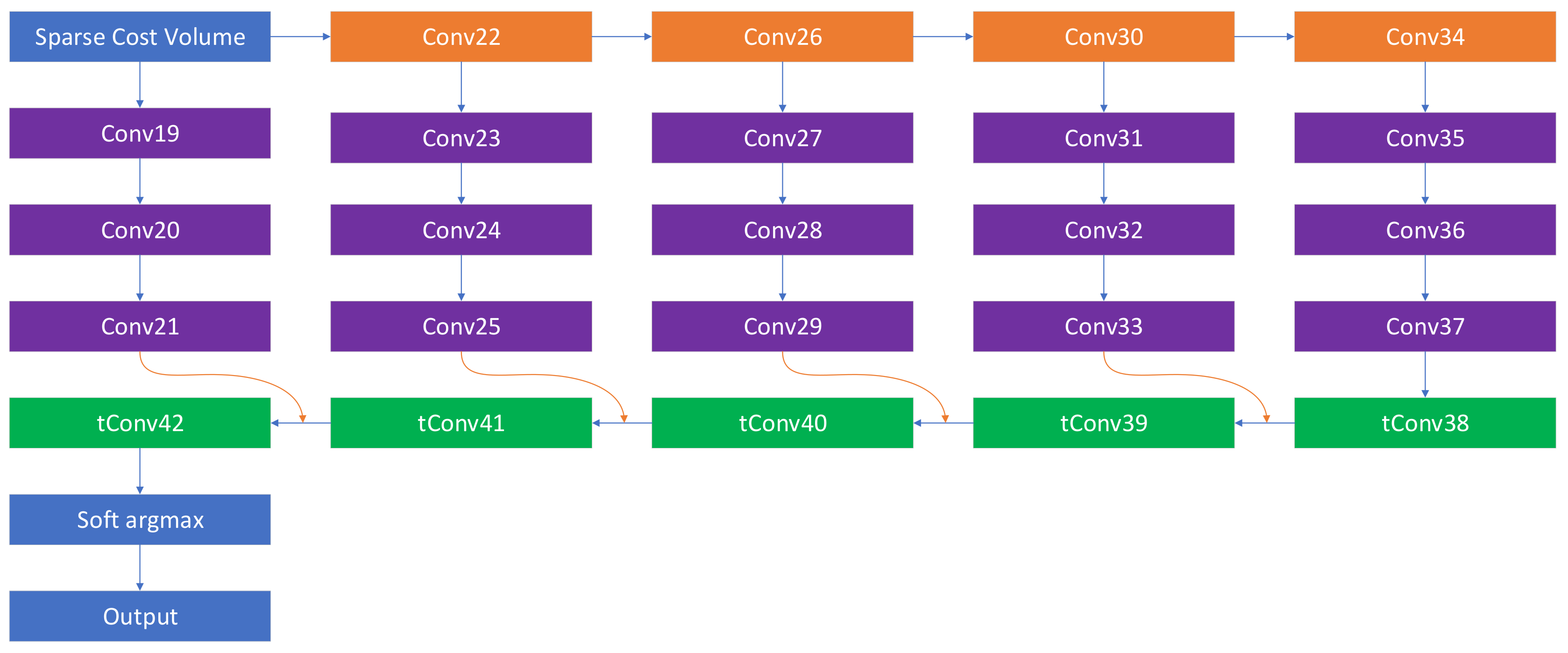
As illustrated in Figure 1 and Table 1, we use an hour-glass structure, which utilizes a series of down-sampling and up-sampling to extract features [24,25]. Figure 4 provides an intuitive view of our network. Each down-sampling layer is followed with a similarity evaluation branch. To make the similarity evaluation more effective, each similarity evaluation branch consists of three convolutional layers. Then, evaluated similarity maps are up-sampled, and added to the similarity maps with the same resolution, and finally up-sampled until they have the same resolution with input stereo images. The layers with lower resolution tend to evaluate global features similarly, while the layers with higher resolution tend to evaluate local features similarly. Combining these similarity maps helps our network give a more comprehensive evaluation using both local and global features.

Figure 4. Structure of our Similarity Evaluation Network. Orange blocks represent down-sampling layers. Green blocks represent up-sampling layers. Purple blocks represent similarity evaluation branches. Orange links represent residual links.

Since $\frac{1}{6}Disparity$ is moved to the $Batchsize$ dimension, all disparity pairs are processed independently. To give an absolute similarity, we removed the weight normalization and ReLU from the output layer. In our feature extraction, we train the network to compress the features of adjacent pixels to one pixel. Then, the features are processed in an encoded way. We decode it in the output layer of our network to get full disparities. The output similarity map has shape [$\frac{1}{6}Disparity$, 6, $Height$, $Width$].

3.4. Loss Function

We use soft argmax to estimate disparities, as similar to [8,26]. This gives our network the ability to achieve sub-pixel accuracy. Before applying soft argmax, we merge the first two dimensions of the similarity map to make a shape of [$Disparity$, $Height$, $Width$]. The predicted disparity $\widehat{D}$ is the weighted average of all possible disparities as

$$\widehat{D}=\sum _{d=0}^{D_{max}}d·\frac{ex{p}^{s_d}}{{\sum }_{d=0}^{D_{max}}ex{p}^{s_d}}$$

(1)

where max possible disparity $D_{max}$ equals to $Disparity-1$ and $s_d$ represents the similarity of disparity d.

We train our model with supervised learning using ground truth disparity data. When using LIDAR to generate the ground truth values such as KITTI dataset [27,28], these labels may be sparse. Therefore, we use the average of the absolute error between the ground truth disparity $D_n$ and the predicted disparity ${\widehat{D}}_n$ as

$$Loss=\frac{1}{N}\sum _{n=1}^N|D_n-{\widehat{D}}_n|$$

(2)

where N is the count of pixels in the image.

3.5. Weight Normalization

Most of neural networks for stereo matching utilize batch normalization to improve the performance. The batch normalization usually performs well for various recognition tasks. However, neural networks for stereo matching are usually too big, which leads to a small $Batchsize$ during training. For example, the $Batchsize$ is lower than 4 in most of the networks [8,13,15,16]. Moreover, the distribution of dataset is usually uneven, especially when the dataset is small. In these situations, batch normalization is not a suitable choice because it fails to adapt to some images in the dataset.

In our network, we propose to use weight normalization in all of the processes. As described in [9], the weight normalization has the following advantages: (1) it does not introduce any dependencies between the samples in a minibatch; (2) it is not sensitive to noise; (3) it has lower computational overhead. This helps our network perform better on the datasets. In Section 4.4, we show the advantages after using weight normalization.

4. Experiments

We evaluated our SCV-Net on the Scene Flow [7] and KITTI 2015 [28] datasets. To achieve better performance, we first trained our network on the Scene Flow dataset. Then, we fine-tuned it with the KITTI dataset.

4.1. Implementation Detail

We implemented our model in PyTorch as follows. The network was randomly initialized. Our model was optimized with RMSProp [29] using a multistep learning rate. Specifically, to train the network with the Scene Flow dataset, the learning rate was set to $1\times {10}^{-4}$ for all 210k iterations. For the fine-tuning with the KITTI 2015 dataset, the learning rate was initially set to $2\times {10}^{-4}$ and then reduced by a half at the 20k-th and 40k-th iterations, and finally the training was stopped at the 60k-th iteration.

We trained our network with the $Batchsize$ of 1 using a $768\times 320$ image pair randomly cropped from the inputs. Before inputting to the network, we normalized each image pair such that the pixel intensities ranged from −1 to 1. Specifically, we performed data augmentation on the KITTI 2015 dataset to improve the adaptability of our network.

For both Scene Flow and KITTI 2015 datasets, $Disparity$ was set to 192. The whole training took about 21 h on a single NVIDIA GTX 1080Ti GPU. It should be noted that the maximum disparity in the datasets was larger than 192. To train the network correctly, we discarded all pixels with disparities out of range [0, 192).

4.2. Computational Efficiency

We implemented the GC-Net and our SCV-Net in the same environment. The two networks were both evaluated on a single NVIDIA 1080Ti GPU. The computational overhead of two networks is described in Table 2. When processing the same data, our SCV-Net saved more than $73.08\%$ GPU memory and $61.11\%$ runtime comparing to the GC-Net. This significant enhancement comes from our efficient sparse cost volume. In addition, experiments in Section 4.3 indicate that our sparse cost volume did not harm the accuracy.

Table 2. Computational overhead of GC-Net and SCV-Net in processing a 1216 × 352 image pair on a single NVIDIA GTX 1080Ti.

	GPU Memory	Runtime
GC-Net	10.4 G	0.90 s
Ours	2.8 G	0.35 s

4.3. Benchmark Results

First, we validated our network on the testing set of Scene Flow dataset. We evaluated end point error (EPE) and pixel percentages with errors larger than 1, 3 and 5 pixels (1PE, 3PE and 5PE). As indicated in Table 3, our network surpassed the GC-Net [8] in all indexes except EPE by a noteworthy margin. As described in Section 4.1, a part of the Scene Flow dataset has disparities larger than 192. We discarded these pixels during training, which led to worse performance on these regions when testing, making the EPE which measures the average error larger. Note that the GPU memory cost and processing time of the GC-Net are absent in Table 3. This is because the image size (960 × 540) is too big, which cannot be processed on a single NVIDIA GTX 1080Ti. The result of GC-Net is quoted from its original paper [8].

Table 3. Results on the Scene Flow dataset.

	≥ 1 px	≥ 3 px	≥ 5 px	EPE	GPU	Time
GC-Net [8]	16.90%	9.34%	7.22%	2.51	-	-
Ours-S2	12.87%	5.04%	3.87%	4.05	4.26 G	0.54 s
Ours-S3	11.36%	5.64%	4.32%	4.07	3.51 G	0.41 s
Ours-S3-BN	11.16%	5.59%	4.34%	4.12	4.00 G	0.41 s
Ours-S4	23.44%	11.38%	4.53%	4.52	2.81 G	0.34 s

Next, we investigated the performance of our network with different stride parameter S for constructing the sparse cost volume. As described in Table 3, Ours-S2, which has a stride of 2, has a better performance on 3PE and 5PE, but is larger and slower. Ours-S4 performs worse on 1PE and 3PE, but has a reasonable performance on 5PE in practice with small memory use and faster computation. The 1PE and 3PE of Ours-S4 have been worse than the GC-Net, so it is not necessary to test with $S>4$. By introducing the stride parameter, we can control the balance between accuracy, memory use and computational cost. Since the performance of Ours-S3 can be balanced, we choose it for the following experiments.

In addition, as shown in Table 3, we investigated how much the weight normalization improved on performance. Ours-S3-BN, which used the batch normalization, surpassed Ours-S3 partly in accuracy. However, using the batch normalization increased $14\%$ GPU memory cost. Moreover, as discussed in Section 4.4, using weight normalization can achieve better performance on dim and noise regions. For these reasons, we decided to use weight normalization in our network.

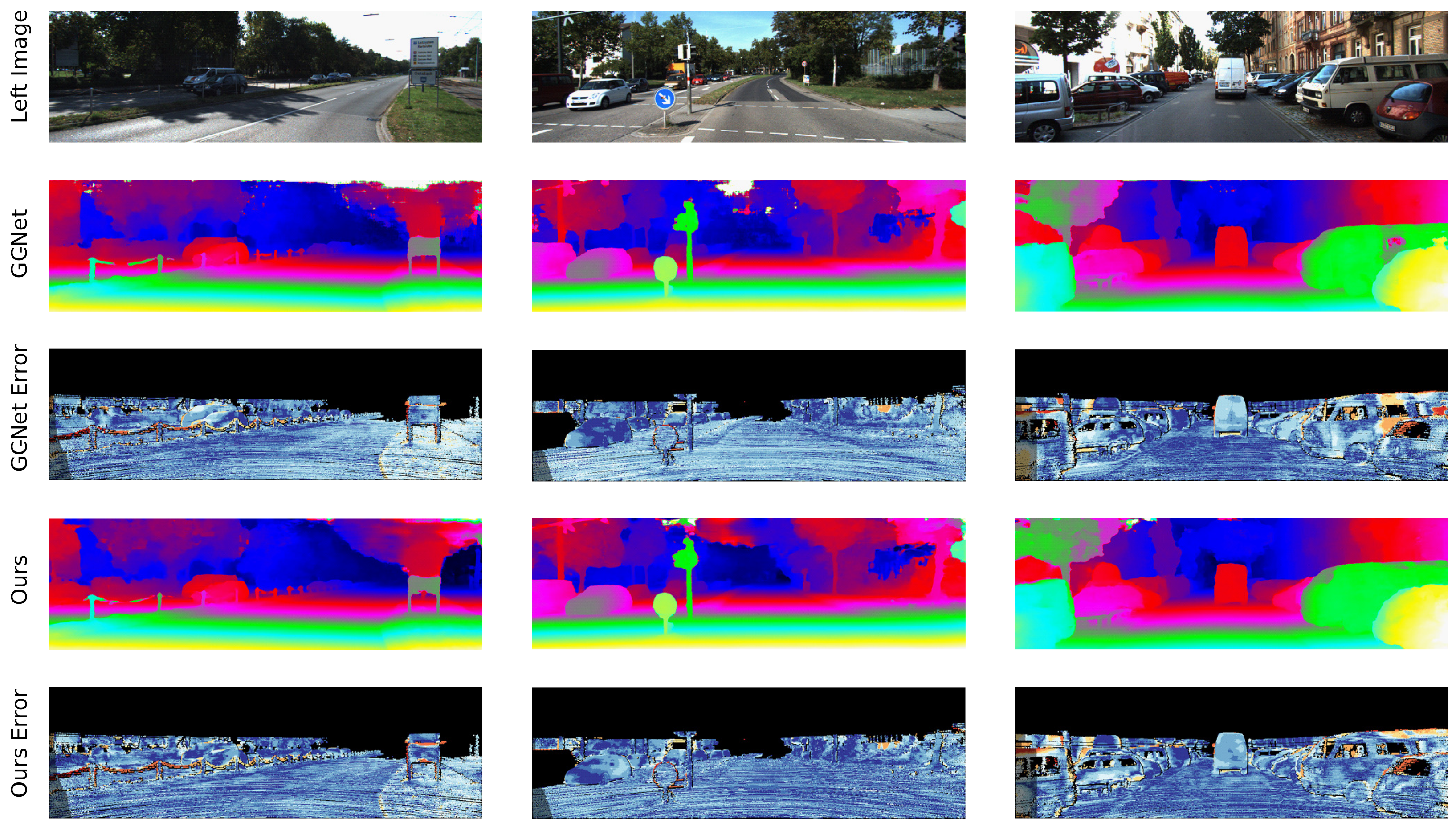
Finally, we evaluated our network (Ours-S3) on the KITTI 2015 benchmark [28]. Figure 5 illustrates the results, and Table 4 provides a detailed comparison. The Foreground index refers to dynamic object pixels such as vehicles and pedestrians. The Background refers to static object pixels such as streets and trees while Overall refers to all pixels. The results show the percentage of pixels which have error greater than 3 pixels over all 200 test image pairs. The Runtime index refers to the average processing time. As shown in Table 4, our network surpassed the GC-Net in almost all indexes.

Figure 5. Results on KITTI 2015 stereo benchmark (include occluded pixels). Our network has better results in the foreground, which corresponds to cars and pedestrians.

Table 4. Results on the KITTI 2015 stereo benchmark.

	Foreground	Background	Overall	Runtime
All pixels (include occluded pixels)
GC-Net [8]	6.16%	2.21%	2.87%	0.90 s
Ours-S3	4.53%	2.22%	2.61%	0.36 s
Only non-occluded pixels
GC-Net [8]	5.58%	2.02%	2.61%	0.90 s
Ours-S3	4.28%	2.04%	2.41%	0.36 s

4.4. Discussions

Stereo matching at dim and noise regions have been an issue for outdoor applications. In our experiments, the GC-Net cannot perform well on these regions. As discussed in Section 3.5, the commonly used batch normalization has poor performance when the $Batchsize$ is too small. As illustrated in Figure 6, our network Ours-S3, which used weight normalization, performed well at these ill-posed regions. In other hand, Ours-S3-BN, which used batch normalization, has similar results with the GC-Net. We also evaluated the GC-Net with weight normalization, it overcomes the limitations of dim lighting and sensor noise regions as well.

Figure 6. Results at dim and noise regions. The top one is in the training set, while the bottom one is in the testing set.

There are still some issues left for further improvements. As illustrated in the top of Figure 7, our network still cannot deal with specular reflection well. In some complex conditions, for example, the object occlusion happens at a texture-less region; our network may fail to separate the foreground and the background, which leads to wrong estimation. As shown in Figure 7 Bottom, our network failed to separate the pedestrians and the street.

Figure 7. Failure examples. Our network still cannot deal with specular reflection and object occlusion well.

5. Conclusions

In this paper, we propose the SCV-Net that contains a sparse cost volume, which saves more than $73.08\%$ GPU memory and $61.11\%$ runtime, compared with the GC-Net. By parameterizing the stride of sparse cost volume, the network could achieve higher accuracy or become faster and smaller. Moreover, we use the weight normalization to settle the problem on processing dim and noise regions. Our network can finally satisfy the requirement of most applications in practice.

References

1. Newcombe, R.A.; Izadi, S.; Hilliges, O.; Molyneaux, D.; Kim, D.; Davison, A.J.; Kohi, P.; Shotton, J.; Hodges, S.; Fitzgibbon, A. KinectFusion: Real-time dense surface mapping and tracking. In Proceedings of the 10th IEEE international symposium on IEEE Mixed and augmented reality (ISMAR), Basel, Switzerland, 26–29 October 2011; pp. 127–136. [Google Scholar]
2. Helmer, S.; Lowe, D. Using stereo for object recognition. In Proceedings of the 2010 IEEE International Conference on Robotics and Automation, Anchorage, AK, USA, 3–7 May 2010; pp. 3121–3127. [Google Scholar]
3. Howard, A. Real-time stereo visual odometry for autonomous ground vehicles. In Proceedings of the IEEE/RSJ 2008 International Conference on Intelligent RObots and Systems, Nice, France, 22–26 September 2008; pp. 3946–3952. [Google Scholar]
4. Scharstein, D.; Szeliski, R. A taxonomy and evaluation of dense two-frame stereo correspondence algorithms. Int. J. Comput. Vis. 2002, 47, 7–42. [Google Scholar] [CrossRef]
5. Zbontar, J.; LeCun, Y. Computing the stereo matching cost with a convolutional neural network. In Proceedings of the IEEE Conference on Computer Vision and Pattern Recognition, Boston, MA, USA, 7–12 June 2015; pp. 1592–1599. [Google Scholar]
6. Luo, W.; Schwing, A.G.; Urtasun, R. Efficient deep learning for stereo matching. In Proceedings of the IEEE Conference on Computer Vision and Pattern Recognition, Las Vegas, NV, USA, 26 June–1 July 2016; pp. 5695–5703. [Google Scholar]
7. Mayer, N.; Ilg, E.; Hausser, P.; Fischer, P.; Cremers, D.; Dosovitskiy, A.; Brox, T. A large dataset to train convolutional networks for disparity, optical flow, and scene flow estimation. In Proceedings of the IEEE Conference on Computer Vision and Pattern Recognition, Las Vegas, NV, USA, 26 June–1 July 2016; pp. 4040–4048. [Google Scholar]
8. Kendall, A.; Martirosyan, H.; Dasgupta, S.; Henry, P.; Kennedy, R.; Bachrach, A.; Bry, A. End-to-end learning of geometry and context for deep stereo regression. arXiv, 2017; arXiv:1703.04309. [Google Scholar]
9. Salimans, T.; Kingma, D.P. Weight normalization: A simple reparameterization to accelerate training of deep neural networks. In Advances in Neural Information Processing Systems; MIT Press: Cambridge, MA, USA, 2016; pp. 901–909. [Google Scholar]
10. Zagoruyko, S.; Komodakis, N. Learning to compare image patches via convolutional neural networks. In Proceedings of the IEEE Conference on Computer Vision and Pattern Recognition, Boston, MA, USA, 7–12 June 2015; pp. 4353–4361. [Google Scholar]
11. Seki, A.; Pollefeys, M. Sgm-nets: Semi-global matching with neural networks. In Proceedings of the 2017 IEEE Conference on Computer Vision and Pattern Recognition Workshops (CVPRW), Honolulu, HI, USA, 1 July 2017; pp. 21–26. [Google Scholar]
12. Gidaris, S.; Komodakis, N. Detect, replace, refine: Deep structured prediction for pixel wise labeling. In Proceedings of the IEEE Conference on Computer Vision and Pattern Recognition, Honolulu, HI, USA, 21–26 July 2017; pp. 5248–5257. [Google Scholar]
13. Pang, J.; Sun, W.; Ren, J.; Yang, C.; Yan, Q. Cascade residual learning: A two-stage convolutional neural network for stereo matching. In Proceedings of the International Conference on Computer Vision-Workshop on Geometry Meets Deep Learning (ICCVW 2017), Venice, Italy, 28 October 2017; Volume 3. [Google Scholar]
14. Jie, Z.; Wang, P.; Ling, Y.; Zhao, B.; Wei, Y.; Feng, J.; Liu, W. Left-Right Comparative Recurrent Model for Stereo Matching. arXiv, 2018; arXiv:1804.00796. [Google Scholar]
15. Liang, Z.; Feng, Y.; Guo, Y.; Liu, H. Learning for Disparity Estimation through Feature Constancy. arXiv, 2017; arXiv:1712.01039. [Google Scholar]
16. Chang, J.R.; Chen, Y.S. Pyramid Stereo Matching Network. arXiv, 2018; arXiv:1803.08669. [Google Scholar]
17. Wang, L.; Jin, H.; Yang, R. Search Space Reduction for MRF Stereo. European Conference on Computer Vision; Springer: Berlin, Germany, 2008; pp. 576–588. [Google Scholar]
18. Veksler, O. Reducing Search Space for Stereo Correspondence with Graph Cuts. In Proceedings of the British Machine Vision Conference (BMVC), Citeseer, Edinburgh, UK, 4–7 September 2006; pp. 709–718. [Google Scholar]
19. Geiger, A.; Roser, M.; Urtasun, R. Efficient large-scale stereo matching. In Computer Vision–ACCV 2010; Springer: Berlin, Germany, 2010; pp. 25–38. [Google Scholar]
20. Gürbüz, Y.Z.; Alatan, A.A.; Çığla, C. Sparse recursive cost aggregation towards O (1) complexity local stereo matching. In Proceedings of the 23rd Signal Processing and Communications Applications Conference (SIU), Malatya, Turkey, 16–19 May 2015; pp. 2290–2293. [Google Scholar]
21. Khamis, S.; Fanello, S.; Rhemann, C.; Kowdle, A.; Valentin, J.; Izadi, S. StereoNet: Guided Hierarchical Refinement for Real-Time Edge-Aware Depth Prediction. In Proceedings of the European Conference on Computer Vision (ECCV), Munich, Germany, 8–14 September 2018; pp. 573–590. [Google Scholar]
22. Huang, G.; Liu, Z.; Weinberger, K.Q.; van der Maaten, L. Densely connected convolutional networks. In Proceedings of the IEEE Conference on Computer Vision and Pattern Recognition, Honolulu, HI, USA, 21–26 July 2017; Volume 1, p. 3. [Google Scholar]
23. He, K.; Zhang, X.; Ren, S.; Sun, J. Deep residual learning for image recognition. In Proceedings of the IEEE Conference on Computer Vision and Pattern Recognition, Las Vegas, NV, USA, 26 June–1 July 2016; pp. 770–778. [Google Scholar]
24. Dosovitskiy, A.; Fischer, P.; Ilg, E.; Hausser, P.; Hazirbas, C.; Golkov, V.; van der Smagt, P.; Cremers, D.; Brox, T. Flownet: Learning optical flow with convolutional networks. In Proceedings of the IEEE International Conference on Computer Vision, Washington, DC, USA, 7–13 December 2015; pp. 2758–2766. [Google Scholar]
25. Ilg, E.; Mayer, N.; Saikia, T.; Keuper, M.; Dosovitskiy, A.; Brox, T. Flownet 2.0: Evolution of optical flow estimation with deep networks. In Proceedings of the IEEE Conference on Computer Vision and Pattern Recognition (CVPR), Honolulu, HI, USA, 21–26 July 2017; Volume 2. [Google Scholar]
26. Bahdanau, D.; Cho, K.; Bengio, Y. Neural machine translation by jointly learning to align and translate. arXiv, 2014; arXiv:1409.0473. [Google Scholar]
27. Geiger, A.; Lenz, P.; Urtasun, R. Are we ready for autonomous driving? the kitti vision benchmark suite. In Proceedings of the 2012 IEEE Conference on Computer Vision and Pattern Recognition, Providence, RI, USA, 16–21 June 2012; pp. 3354–3361. [Google Scholar]
28. Menze, M.; Geiger, A. Object scene flow for autonomous vehicles. In Proceedings of the IEEE Conference on Computer Vision and Pattern Recognition, Boston, MA, USA, 7 June–12 June 2015; pp. 3061–3070. [Google Scholar]
29. Tieleman, T.; Hinton, G. Lecture 6.5-rmsprop: Divide the gradient by a running average of its recent magnitude. COURSERA Neural Netw. Mach. Learn. 2012, 4, 26–31. [Google Scholar]
Article Metrics
Citations
Article Access Statistics
Multiple requests from the same IP address are counted as one view.