Aboveground Tree Biomass Estimation of Sparse Subalpine Coniferous Forest with UAV Oblique Photography


Abstract
1. Introduction
2. Study Area and Data
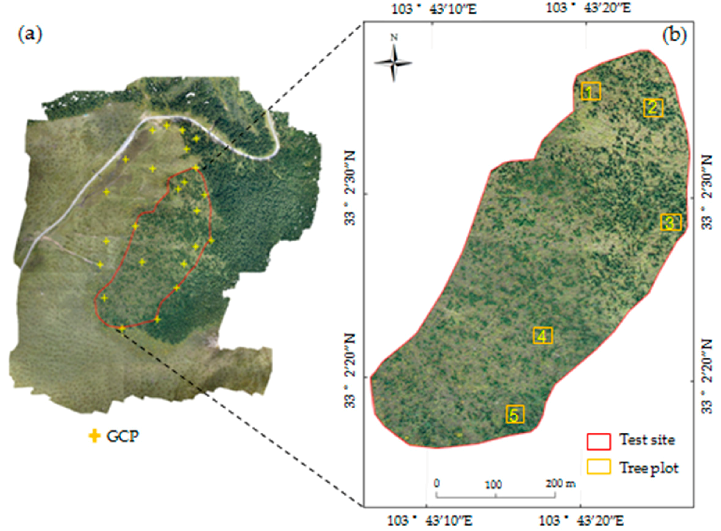
2.1. Study Area
2.2. UAV Data
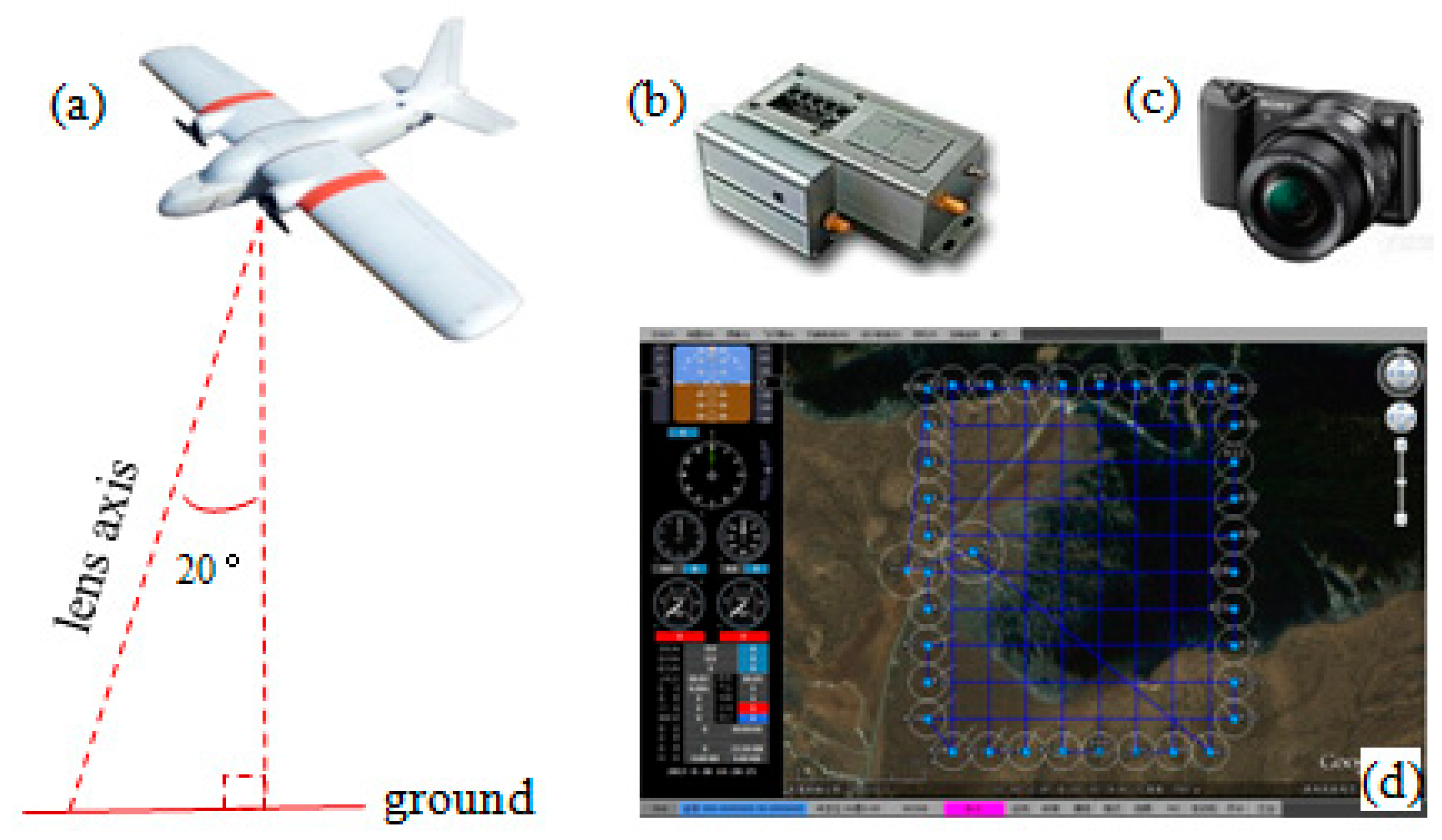
2.2.1. UAV System
2.2.2. DOM of Test Site
2.3. Field Data
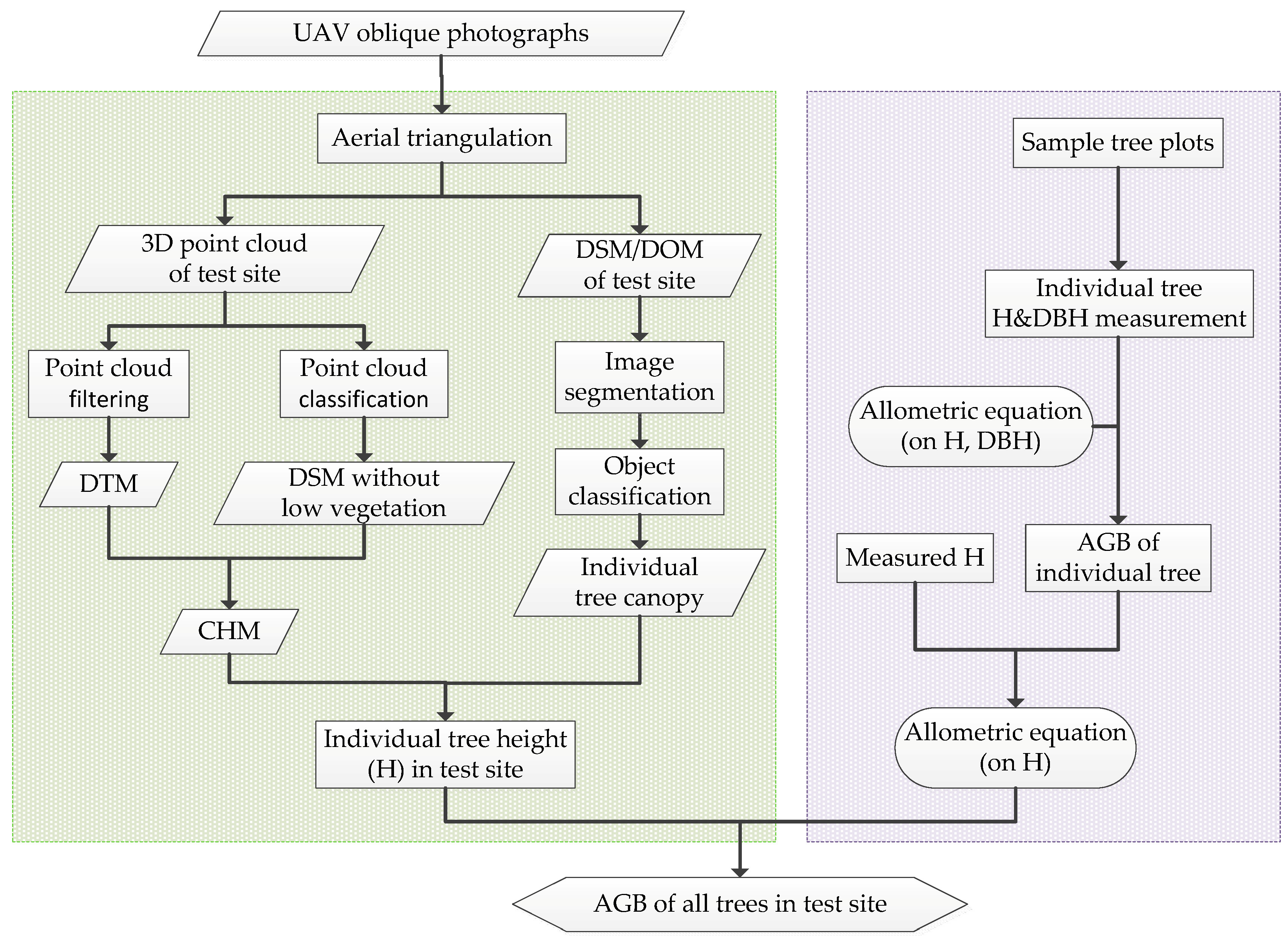
3. Methodology
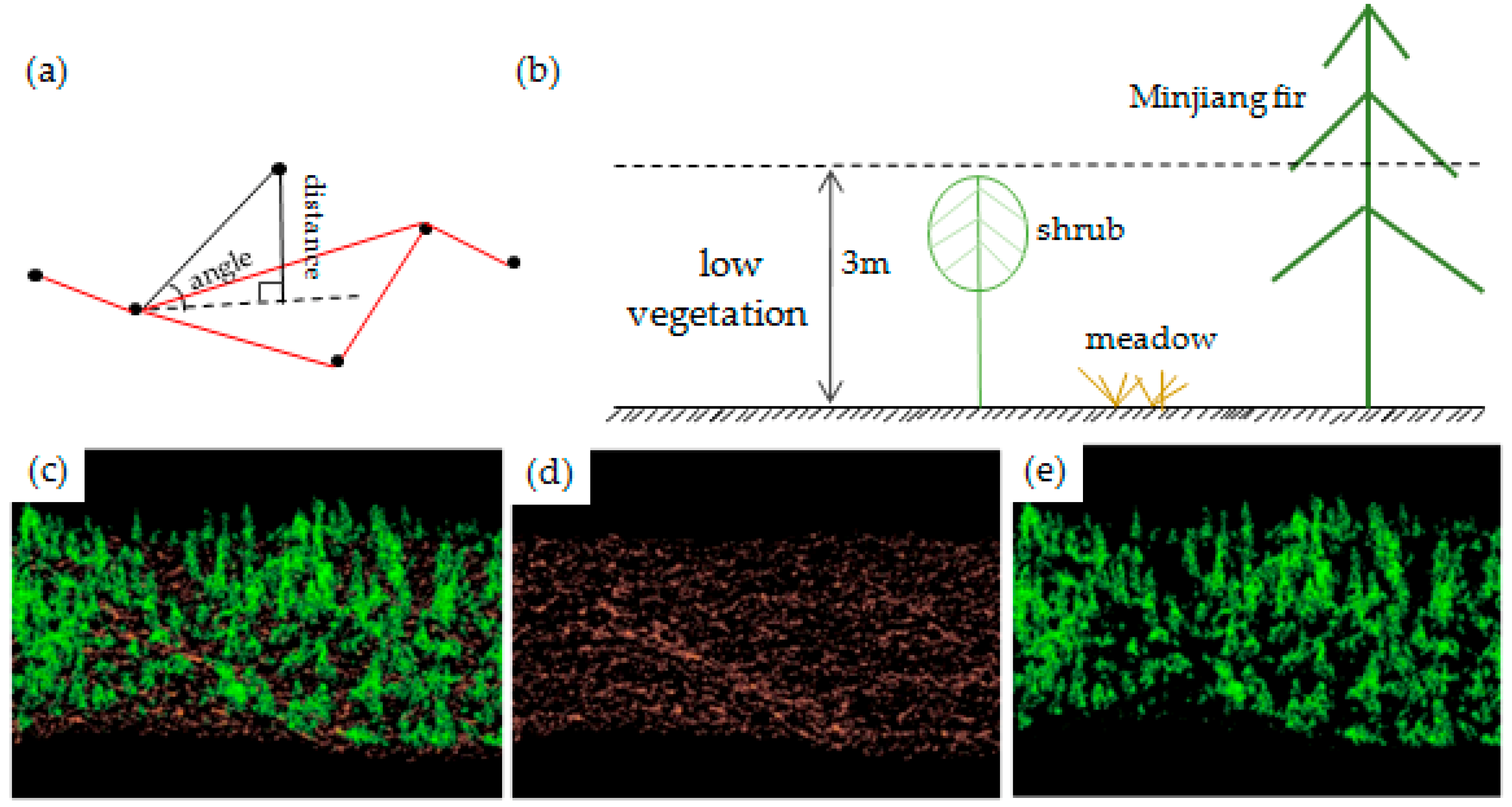
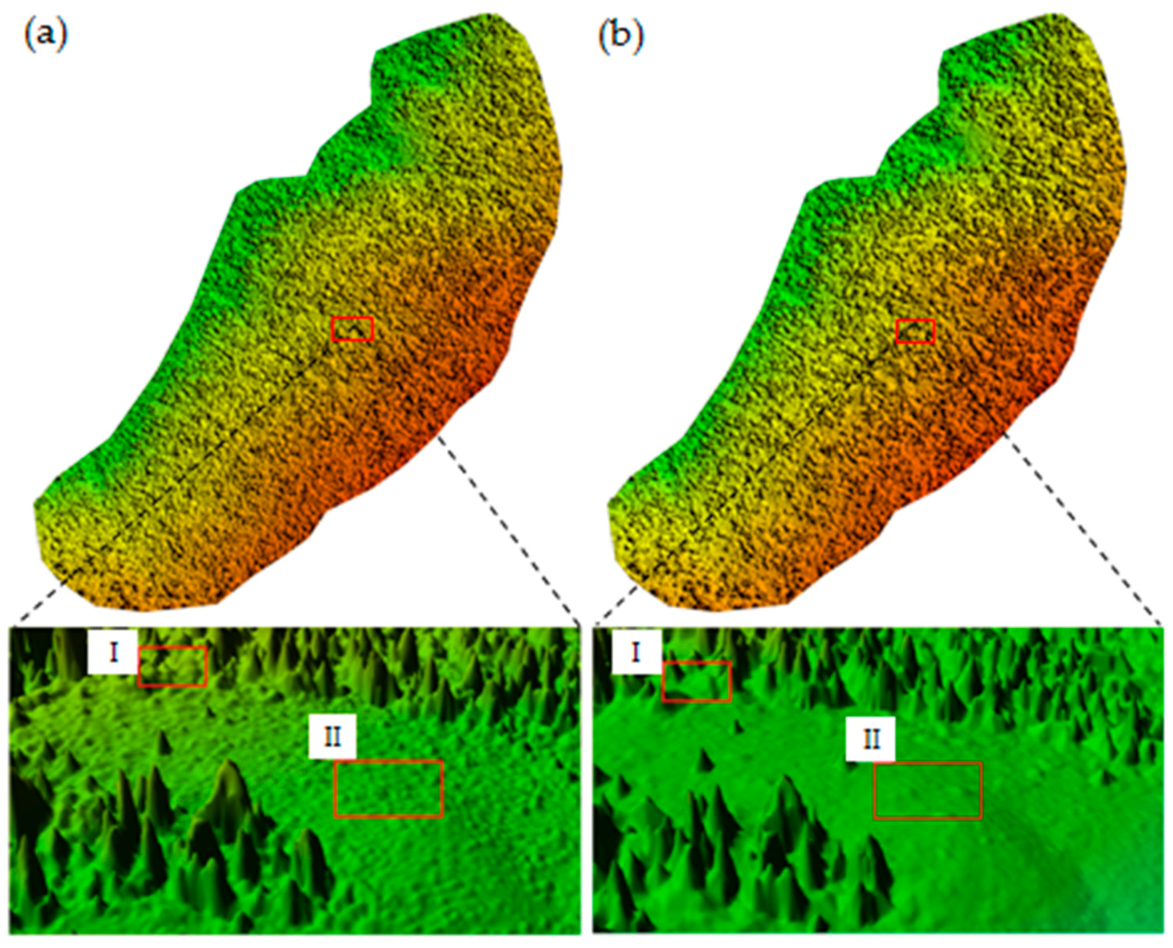
3.1. Point Cloud Acquisition and Denoising
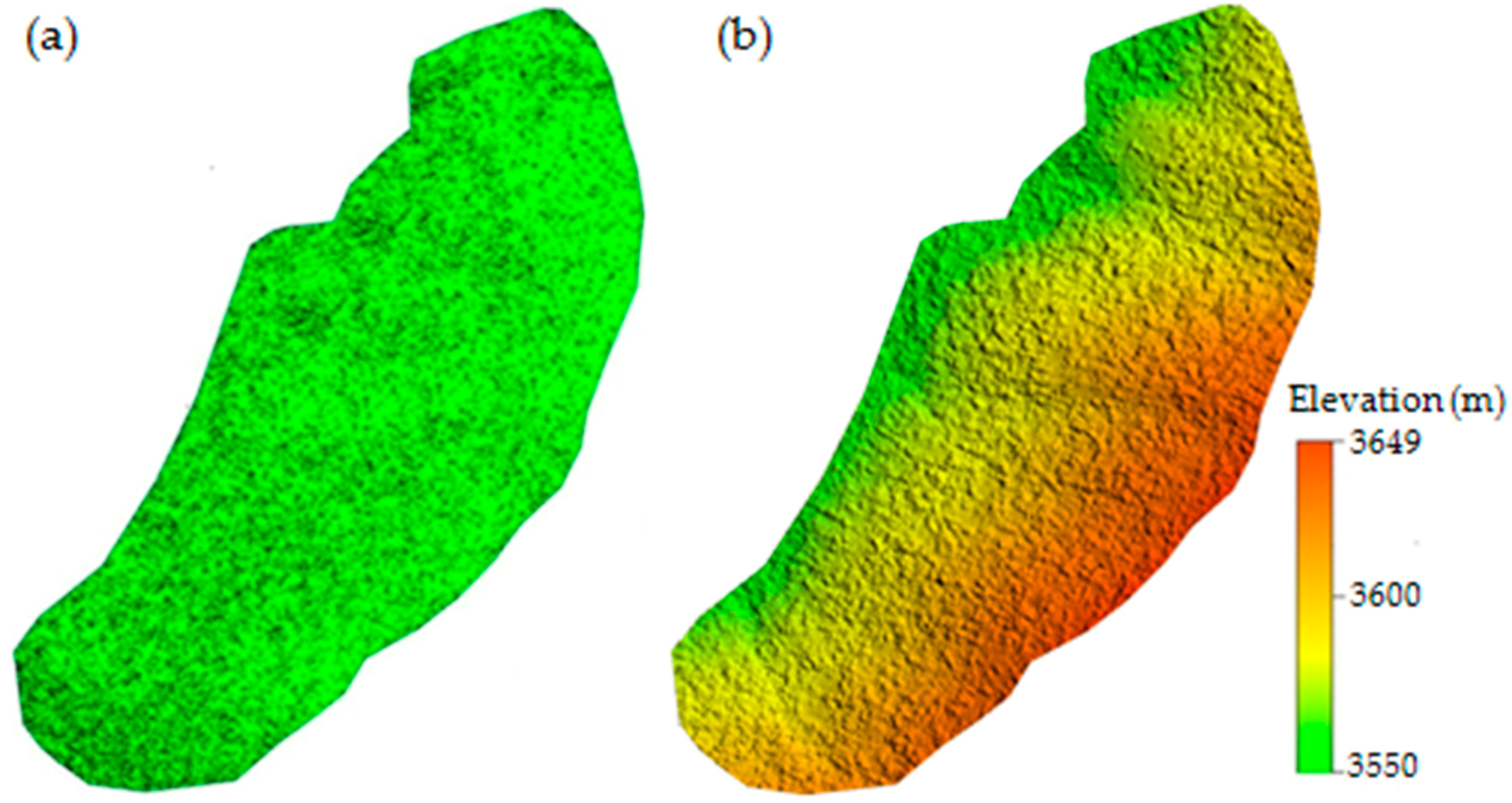
3.2. CHM Computation
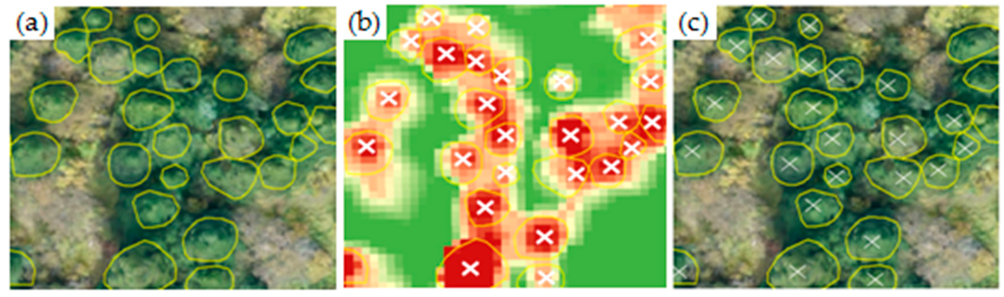
3.3. Extraction of Individual Tree Canopy and Height
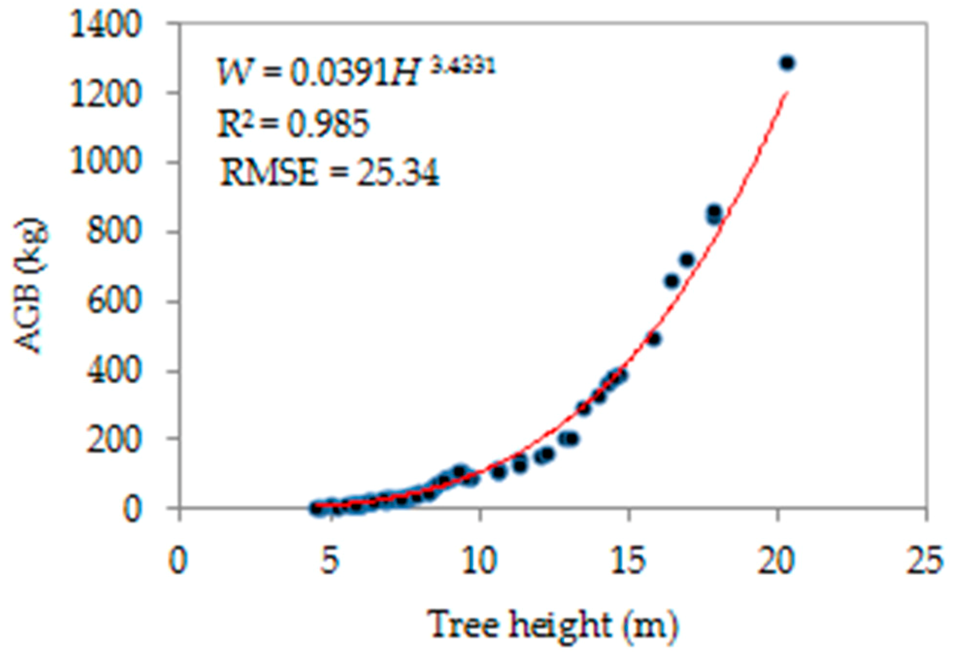
3.4. Allometric Equation on Tree Height
4. Results
4.1. Computed CHM
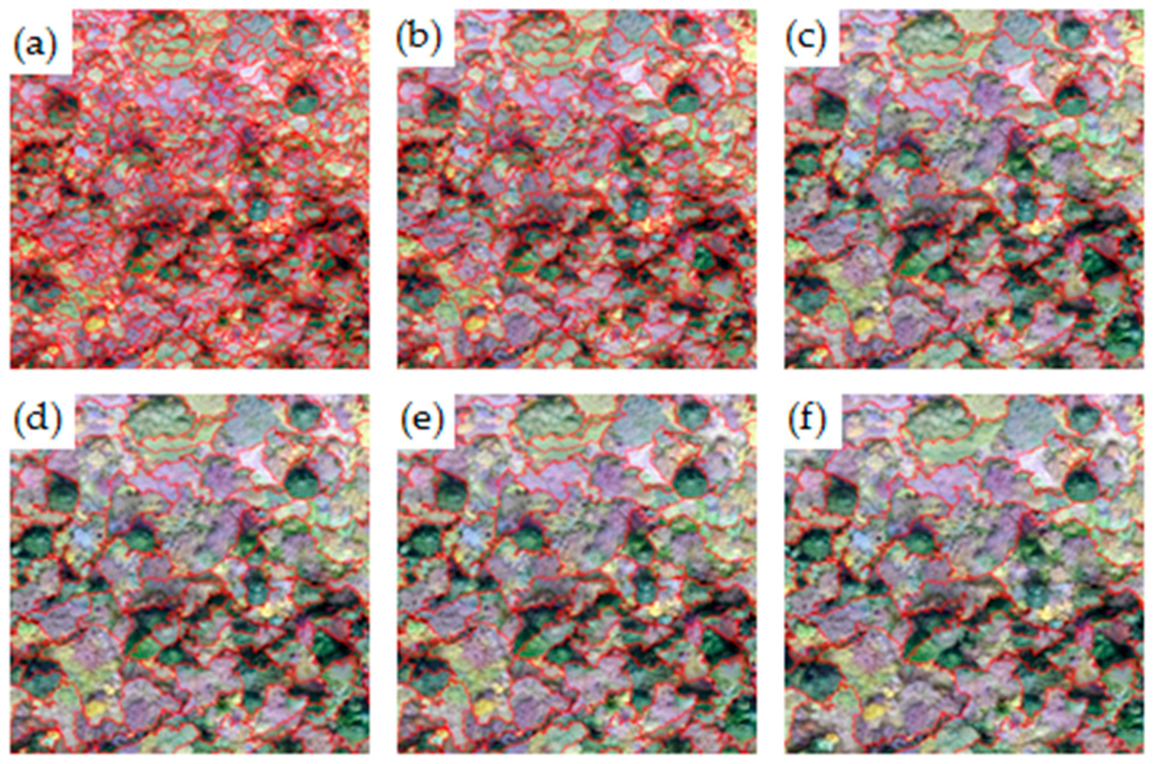
4.2. Segmented Tree Canopy Outlines
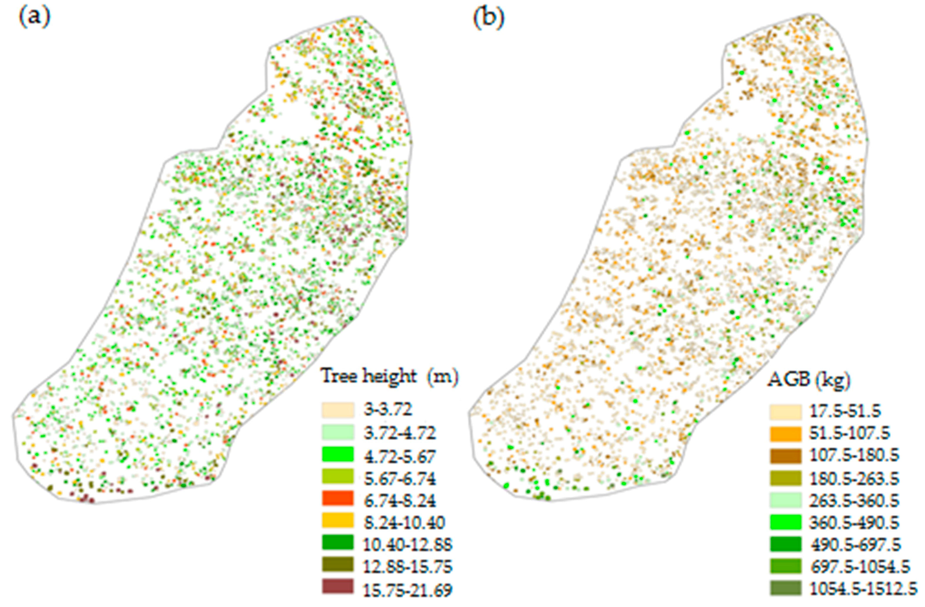
4.3. Extracted Individual Tree Heights
4.4. Estimated AGB
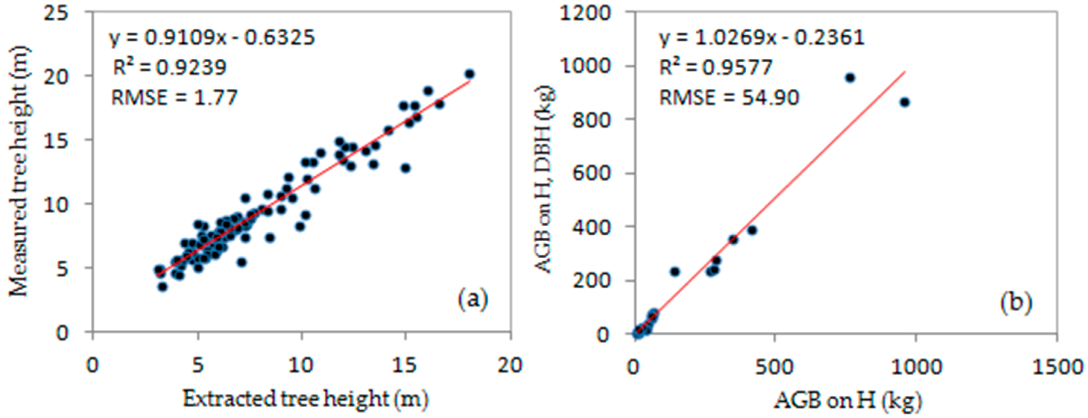
4.5. Accuracy Assessment
5. Discussion
6. Conclusions
Author Contributions
Funding
Acknowledgments
Conflicts of Interest
Appendix A

| Tree No. | Height (m) | DBH (cm) | Tree No. | Height (m) | DBH (cm) | Tree No. | Height (m) | DBH (cm) |
| 1-1 1 | 7.41 | 13.4 | 2-1 | 5.9 | 11.2 | 3-1 | 17.83 | 51.7 |
| 1-2 | 7.15 | 14.0 | 2-2 | 4.95 | 10.5 | 3-2 | 12.2 | 25.7 |
| 1-3 | 10.63 | 23.1 | 2-3 | 17.86 | 51.3 | 3-3 | 7.35 | 14.4 |
| 1-4 | 12.0 | 24.9 | 2-4 | 8.5 | 19.4 | 3-4 | 8.24 | 17.0 |
| 1-5 | 9.72 | 21.5 | 2-5 | 13.44 | 33.4 | 3-5 | 16.36 | 46.8 |
| 1-6 | 8.37 | 17.9 | 2-6 | 15.8 | 40.8 | 3-6 | 5.2 | 8.9 |
| 1-7 | 9.35 | 23.4 | 2-7 | 14.25 | 36.4 | 3-7 | 14.51 | 37.0 |
| 1-8 | 9.73 | 21.6 | 2-8 | 9.03 | 21.8 | 3-8 | 5.82 | 9.0 |
| 1-9 | 11.3 | 25.0 | 2-9 | 9.2 | 22.6 | 3-9 | 7.95 | 16.4 |
| 1-10 | 8.34 | 17.7 | 2-10 | 6.78 | 12.6 | 3-10 | 12.89 | 28.0 |
| 1-11 | 10.56 | 22.5 | 2-11 | 8.36 | 18.0 | 3-11 | 11.33 | 23.3 |
| 1-12 | 16.87 | 48.3 | 2-12 | 5.7 | 9.8 | 3-12 | 7.64 | 14.8 |
| 1-13 | 9.45 | 21.1 | 2-13 | 7.45 | 13.9 | 3-13 | 7.65 | 14.9 |
| 1-14 | 7.55 | 14.4 | 2-14 | 7.97 | 16.6 | 3-14 | 7.85 | 15.0 |
| 1-15 | 6.8 | 14.3 | 2-15 | 8.6 | 20.1 | 3-15 | 10.56 | 22.7 |
| 1-16 | 5.84 | 9.1 | 2-16 | 6.37 | 11.6 | 3-16 | 8.86 | 21.9 |
| 3-17 | 8.86 | 21.4 | ||||||
| 3-18 | 6.06 | 11.1 | ||||||
| 3-19 | 6.28 | 13.0 | ||||||
| 3-20 | 4.65 | 8.6 | ||||||
| 3-21 | 14.66 | 37.5 | ||||||
| 3-22 | 6.2 | 12.8 | ||||||
| 3-23 | 6.0 | 11.2 | ||||||
| Tree No. | Height(m) | DBH(cm) | Tree No. | Height(m) | DBH(cm) | |||
| 4-1 | 14.45 | 37.3 | 5-1 | 10.83 | 33.0 | |||
| 4-2 | 13.06 | 28.1 | 5-2 | 7.9 | 15.1 | |||
| 4-3 | 9.26 | 23.5 | 5-3 | 14.1 | 36.2 | |||
| 4-4 | 5.75 | 9.7 | 5-4 | 7.36 | 11.0 | |||
| 4-5 | 8.25 | 17.0 | 5-5 | 14.9 | 36.9 | |||
| 4-6 | 7.13 | 13.9 | 5-6 | 5.0 | 4.8 | |||
| 4-7 | 6.3 | 11.9 | 5-7 | 8.63 | 20.6 | |||
| 4-8 | 14.0 | 35.0 | 5-8 | 3.67 | 5.3 | |||
| 4-9 | 20.3 | 60.2 | 5-9 | 17.74 | 55.0 | |||
| 4-10 | 6.95 | 14.1 | 5-10 | 13.13 | 30.0 | |||
| 4-11 | 6.2 | 12.9 | 5-11 | 13.3 | 30.2 | |||
| 4-12 | 7.3 | 13.2 | 5-12 | 8.4 | 18.0 | |||
| 4-13 | 4.61 | 8.5 | 5-13 | 5.7 | 8.2 | |||
| 4-14 | 6.96 | 14.2 | 5-14 | 8.54 | 20.0 | |||
| 4-15 | 5.92 | 10.9 | 5-15 | 13.35 | 32.6 | |||
| 4-16 | 5.6 | 9.7 | 5-16 | 6.1 | 11.5 | |||
| 4-17 | 6.9 | 15.0 | 5-17 | 7.46 | 9.5 | |||
| 4-18 | 8.8 | 21.2 | 5-18 | 8.5 | 19.3 | |||
| 4-19 | 5.54 | 9.3 | 5-19 | 18.97 | 50.3 | |||
| 4-20 | 6.74 | 13.9 | 5-20 | 6.68 | 12.7 | |||
| 4-21 | 6.45 | 12.3 | 5-21 | 5.1 | 11.0 | |||
| 4-22 | 5.83 | 10.1 | ||||||
| 4-23 | 4.53 | 8.6 | ||||||
| 4-24 | 7.38 | 13.0 |
Appendix B
| GCP # | Lng °E | Lat °N | Elevation (m) |
|---|---|---|---|
| 1 | 103.7226 | 33.0402 | 3632.31 |
| 2 | 103.7223 | 33.0434 | 3571.83 |
| 3 | 103.7235 | 33.0431 | 3598.32 |
| 4 | 103.7238 | 33.0412 | 3639.75 |
| 5 | 103.7213 | 33.0379 | 3654.38 |
| 6 | 103.7218 | 33.0460 | 3528.96 |
| 7 | 103.7211 | 33.0458 | 3524.72 |
| 8 | 103.7211 | 33.0442 | 3533.55 |
| 9 | 103.7225 | 33.0458 | 3539.97 |
| 10 | 103.7231 | 33.0455 | 3523.57 |
| 11 | 103.7227 | 33.0450 | 3555.14 |
| 12 | 103.7231 | 33.0443 | 3573.34 |
| 13 | 103.7226 | 33.0437 | 3566.51 |
| 14 | 103.7232 | 33.0425 | 3594.29 |
| 15 | 103.7231 | 33.0410 | 3634.34 |
| 16 | 103.7222 | 33.0392 | 3648.6 |
| 17 | 103.7197 | 33.0375 | 3619.65 |
| 18 | 103.7189 | 33.0388 | 3572.19 |
| 19 | 103.7187 | 33.0402 | 3539.22 |
| 20 | 103.7190 | 33.0412 | 3538.14 |
| 21 | 103.7206 | 33.0403 | 3581.71 |
| 22 | 103.7203 | 33.0418 | 3554.65 |
| 23 | 103.7190 | 33.0432 | 3516.16 |
| 24 | 103.7199 | 33.0446 | 3519.28 |
References
- McKendry, P. Energy production from biomass (part 1): Overview of biomass. Bioresour. Technol. 2002, 83, 37–46. [Google Scholar] [CrossRef]
- Brahma, B.; Nath, A.J.; Sileshi, G.W.; Das, A.K. Estimating biomass stocks and potential loss of biomass carbon through clear-felling of rubber plantations. Biomass Bioenerg. 2018, 115, 88–96. [Google Scholar] [CrossRef]
- Bonnor, G.M. Estimation versus measurement of tree heights in forest inventories. For. Chron. 1974, 50, 200. [Google Scholar] [CrossRef]
- Brack, C.L. Tree and Forest Measurement; Springer: Berlin/Heidelberg, Germany, 2009. [Google Scholar]
- Zeng, W.S.; Fu, L.Y.; Xu, M.; Wang, X.J.; Chen, Z.X.; Yao, S.B. Developing individual tree-based models for estimating aboveground biomass of five key coniferous species in China. J. For. Res. 2018, 29, 1251–1261. [Google Scholar] [CrossRef]
- Colgan, M.S.; Asner, G.P.; Swemmer, T. Harvesting tree biomass at the stand level to assess the accuracy of field and airborne biomass estimation in savannas. Ecol. Appl. 2013, 23, 1170–1184. [Google Scholar] [CrossRef] [PubMed]
- Schlund, M.; Davidson, M.W.J. Aboveground forest biomass estimation combining l- and p-band sar acquisitions. Remote Sens. 2018, 10, 1151. [Google Scholar] [CrossRef]
- Shao, Z.F.; Zhang, L.J. Estimating forest aboveground biomass by combining optical and sar data: A case study in Genhe, inner Mongolia, China. Sensors 2016, 16, 834. [Google Scholar] [CrossRef] [PubMed]
- Beaudoin, A.; Letoan, T.; Goze, S.; Nezry, E.; Lopes, A.; Mougin, E.; Hsu, C.C.; Han, H.C.; Kong, J.A.; Shin, R.T. Retrieval of forest biomass from sar data. Int. J. Remote Sens. 1994, 15, 2777–2796. [Google Scholar] [CrossRef]
- Berninger, A.; Lohberger, S.; Stangel, M.; Siegert, F. Sar-based estimation of above-ground biomass and its changes in tropical forests of kalimantan using l- and c-band. Remote Sens. 2018, 10, 831. [Google Scholar] [CrossRef]
- Santi, E.; Paloscia, S.; Pettinato, S.; Fontanelli, G.; Mura, M.; Zolli, C.; Maselli, F.; Chiesi, M.; Bottai, L.; Chirici, G. The potential of multifrequency sar images for estimating forest biomass in mediterranean areas. Remote Sens. Environ. 2017, 200, 63–73. [Google Scholar] [CrossRef]
- Sheridan, R.D.; Popescu, S.C.; Gatziolis, D.; Morgan, C.L.S.; Ku, N.W. Modeling forest aboveground biomass and volume using airborne lidar metrics and forest inventory and analysis data in the pacific northwest. Remote Sens. 2015, 7, 229–255. [Google Scholar] [CrossRef]
- Hansen, E.H.; Gobakken, T.; Bollandsas, O.M.; Zahabu, E.; Naesset, E. Modeling aboveground biomass in dense tropical submontane rainforest using airborne laser scanner data. Remote Sens. 2015, 7, 788–807. [Google Scholar] [CrossRef]
- Pflugmacher, D.; Cohen, W.; Kennedy, R.; Lefsky, M. Regional applicability of forest height and aboveground biomass models for the geoscience laser altimeter system. For. Sci. 2008, 54, 647–657. [Google Scholar]
- Wang, D.L.; Xin, X.P.; Shao, Q.Q.; Brolly, M.; Zhu, Z.L.; Chen, J. Modeling aboveground biomass in hulunber grassland ecosystem by using unmanned aerial vehicle discrete lidar. Sensors 2017, 17, 180. [Google Scholar] [CrossRef] [PubMed]
- Lin, J.Y.; Shu, L.; Zuo, H.; Zhang, B.S. Experimental observation and assessment of ice conditions with a fixed-wing unmanned aerial vehicle over yellow river, China. J. Appl. Remote Sens. 2012, 6, 063586. [Google Scholar] [CrossRef]
- Balsi, M.; Esposito, S.; Fallavollita, P.; Nardinocchi, C. Single-tree detection in high-density lidar data from uav-based survey. Eur. J. Remote Sens. 2018, 51, 679–692. [Google Scholar] [CrossRef]
- Sankey, T.; Donager, J.; McVay, J.; Sankey, J.B. Uav lidar and hyperspectral fusion for forest monitoring in the southwestern USA. Remote Sens. Environ. 2017, 195, 30–43. [Google Scholar] [CrossRef]
- Brede, B.; Lau, A.; Bartholomeus, H.M.; Kooistra, L. Comparing riegl ricopter uav lidar derived canopy height and dbh with terrestrial lidar. Sensors 2017, 17, 2371. [Google Scholar] [CrossRef] [PubMed]
- Wallace, L.; Lucieer, A.; Watson, C.; Turner, D. Development of a uav-lidar system with application to forest inventory. Remote Sens. 2012, 4, 1519–1543. [Google Scholar] [CrossRef]
- Guo, Q.; Su, Y.; Hu, T.; Zhao, X.; Wu, F.; Li, Y.; Liu, J.; Chen, L.; Xu, G.; Lin, G.; et al. An integrated uav-borne lidar system for 3D habitat mapping in three forest ecosystems across China. Int. J. Remote Sens. 2017, 38, 2954–2972. [Google Scholar] [CrossRef]
- Wallace, L.; Lucieer, A.; Watson, C.S. Evaluating tree detection and segmentation routines on very high resolution uav lidar data. IEEE Trans. Geosci. Remote 2014, 52, 7619–7628. [Google Scholar] [CrossRef]
- Dempewolf, J.; Nagol, J.; Hein, S.; Thiel, C.; Zimmermann, R. Measurement of within-season tree height growth in a mixed forest stand using uav imagery. Forests 2017, 8, 231. [Google Scholar] [CrossRef]
- Ota, T.; Ogawa, M.; Mizoue, N.; Fukumoto, K.; Yoshida, S. Forest structure estimation from a uav-based photogrammetric point cloud in managed temperate coniferous forests. Forests 2017, 8, 343. [Google Scholar] [CrossRef]
- Gatziolis, D.; Lienard, J.F.; Vogs, A.; Strigul, N.S. 3D tree dimensionality assessment using photogrammetry and small unmanned aerial vehicles. PloS ONE 2015, 10, e0137765. [Google Scholar] [CrossRef] [PubMed]
- Stone, C.; Webster, M.; Osborn, J.; Iqbal, I. Alternatives to lidar-derived canopy height models for softwood plantations: A review and example using photogrammetry. Aust. For. 2016, 79, 271–282. [Google Scholar] [CrossRef]
- Liu, Q.; Li, S.; Li, Z.; Fu, L.; Hu, K. Review on the applications of uav-based lidar and photogrammetry in forestry. Scientia Silvae Sinicae 2017, 53, 134–148. [Google Scholar]
- Ota, T.; Ogawa, M.; Shimizu, K.; Kajisa, T.; Mizoue, N.; Yoshida, S.; Takao, G.; Hirata, Y.; Furuya, N.; Sano, T. Aboveground biomass estimation using structure from motion approach with aerial photographs in a seasonal tropical forest. Forests 2015, 6, 3882–3898. [Google Scholar] [CrossRef]
- Baltsavias, E.P. A comparison between photogrammetry and laser scanning. ISPRS J. Photogramm. Remote Sens. 1999, 54, 83–94. [Google Scholar] [CrossRef]
- Zhang, G.; Liu, S.; Zhang, Y.; Wang, Z.; Miao, N. Biomass carbon density of sub-alpine dark coniferous forest in the upper reaches of minjiang river. Scientia Silvae Sinicae 2008, 44, 1–6. [Google Scholar]
- Yang, W.-Q.; Wang, K.-Y.; Kellomaki, S.; Zhang, J. Annual and monthly variations in litter macronutrients of three subalpine forests in western China. Pedosphere 2006, 16, 788–798. [Google Scholar] [CrossRef]
- Pang, X.Y.; Bao, W.K.; Wu, N. The effects of clear-felling subalpine coniferous forests on soil physical and chemical properties in the eastern tibetan plateau. Soil Use Manag. 2011, 27, 213–220. [Google Scholar] [CrossRef]
- Wang, W. The spatial distribution of ecological community and vegetation restoration in the source region of minjiang river. Chin. Agric. Sci. Bull. 2011, 27, 42–47. [Google Scholar]
- Bentley. Contextcapture User Guide; Bentley: Exton, PA, USA, 2016. [Google Scholar]
- Wolff, K.; Kim, C.; Zimmer, H.; Schroers, C.; Botsch, M.; Sorkinehornung, O.; Sorkinehornung, A. Point cloud noise and outlier removal for image-based 3D reconstruction. In Proceedings of the Fourth International Conference on 3D Vision, Stanford, CA, USA, 25–28 October 2016; pp. 118–127. [Google Scholar]
- Wallace, L.; Lucieer, A.; Malenovsky, Z.; Turner, D.; Vopenka, P. Assessment of forest structure using two uav techniques: A comparison of airborne laser scanning and structure from motion (sfm) point clouds. Forests 2016, 7, 62. [Google Scholar] [CrossRef]
- Wei, L.X.; Yang, B.A.; Jiang, J.P.; Cao, G.Z.; Wu, M.F. Vegetation filtering algorithm for uav-borne lidar point clouds: A case study in the middle-lower yangtze river riparian zone. Int. J. Remote Sens. 2017, 38, 2991–3002. [Google Scholar] [CrossRef]
- Dragut, L.; Tiede, D.; Levick, S.R. Esp: A tool to estimate scale parameter for multiresolution image segmentation of remotely sensed data. Int. J. Geogr. Inf. Sci. 2010, 24, 859–871. [Google Scholar] [CrossRef]
- Trimble. Ecognition Developer 8.9 User Guide; Trimble: Sunnyvale, CA, USA, 2013. [Google Scholar]
- Administration, S.F. Guideline for Metering and Monitoring Carbon Sequestration in Afforestation Projects; China Forestry Publishing House: Beijing, China, 2008. [Google Scholar]
- Terrasolid. Terrascan User’s Guide; Terrasolid: Helsinki, Finland, 2016. [Google Scholar]
- Kim, C.; Sorkine-Hornung, O.; Schroers, C.; Zimmer, H.; Wolff, K.; Botsch, M.; Sorkine-Hornung, A. Point Cloud Noise and Outlier Removal for Image-Based 3D Reconstruction; IEEE: Piscataway, NJ, USA, 2018; pp. 118–127. [Google Scholar]
- Rosnell, T.; Honkavaara, E. Point cloud generation from aerial image data acquired by a quadrocopter type micro unmanned aerial vehicle and a digital still camera. Sensors 2012, 12, 453–480. [Google Scholar] [CrossRef] [PubMed]
- Luo, L.; Zhai, Q.; Su, Y.; Ma, Q.; Kelly, M.; Guo, Q. Simple method for direct crown base height estimation of individual conifer trees using airborne lidar data. Opt. Express 2018, 26, A562–A578. [Google Scholar] [CrossRef] [PubMed]
- Zarco-Tejada, P.J.; Diaz-Varela, R.; Angileri, V.; Loudjani, P. Tree height quantification using very high resolution imagery acquired from an unmanned aerial vehicle (uav) and automatic 3D photo-reconstruction methods. Eur. J. Agron. 2014, 55, 89–99. [Google Scholar] [CrossRef]
- Mohan, M.; Silva, C.A.; Klauberg, C.; Jat, P.; Catts, G.; Cardil, A.; Hudak, A.T.; Dia, M. Individual tree detection from unmanned aerial vehicle (uav) derived canopy height model in an open canopy mixed conifer forest. Forests 2017, 8, 340. [Google Scholar] [CrossRef]
- Jurjević, L.; Balenović, I.; Gašparović, M.; Milas, A.Š.; Marjanović, H. Testing the uav-based point clouds of different densities for tree- and plot-level forest measurements. In Proceedings of the Uas4enviro2018-6th Conference for Unmanned Aerial Systems for Environmental Research, Split, Hrvatska, 27–29 June 2018. [Google Scholar]


| Tree No. | AGB (kg) | Tree No. | AGB (kg) | Tree No. | AGB (kg) | Tree No. | AGB (kg) |
|---|---|---|---|---|---|---|---|
| 1-1 | 30.96 | 2-1 | 17.95 | 3-1 | 861.19 | 4-1 | 386.15 |
| 1-2 | 32.49 | 2-2 | 13.53 | 3-2 | 165.11 | 4-2 | 207.65 |
| 1-3 | 119.15 | 2-3 | 850.18 | 3-3 | 35.13 | 4-3 | 108.21 |
| 1-4 | 153.31 | 2-4 | 69.97 | 3-4 | 53.19 | 4-4 | 13.42 |
| 1-5 | 95.94 | 2-5 | 294.01 | 3-5 | 660.69 | 4-5 | 53.25 |
| 1-6 | 59.4 | 2-6 | 495.67 | 3-6 | 10.41 | 4-6 | 31.98 |
| 1-7 | 108.32 | 2-7 | 364.26 | 3-7 | 381.86 | 4-7 | 21.36 |
| 1-8 | 96.87 | 2-8 | 91.94 | 3-8 | 11.81 | 4-8 | 333.13 |
| 1-9 | 146.07 | 2-9 | 100.02 | 3-9 | 48.12 | 4-9 | 1289.21 |
| 1-10 | 57.97 | 2-10 | 25.43 | 3-10 | 203.78 | 4-10 | 32.07 |
| 1-11 | 112.76 | 2-11 | 59.95 | 3-11 | 128.46 | 4-11 | 24.45 |
| 1-12 | 720.86 | 2-12 | 13.57 | 3-12 | 38.32 | 4-12 | 29.7 |
| 1-13 | 90.26 | 2-13 | 33.31 | 3-13 | 38.85 | 4-13 | 8.55 |
| 1-14 | 36.02 | 2-14 | 49.33 | 3-14 | 40.29 | 4-14 | 32.54 |
| 1-15 | 32.26 | 2-15 | 75.55 | 3-15 | 114.63 | 4-15 | 17.12 |
| 1-16 | 12.09 | 2-16 | 20.58 | 3-16 | 91.1 | 4-16 | 13.09 |
| 3-17 | 87.27 | 4-17 | 35.74 | ||||
| 3-18 | 18.1 | 4-18 | 85.22 | ||||
| 3-19 | 25.1 | 4-19 | 11.99 | ||||
| 3-20 | 8.81 | 4-20 | 30.35 | ||||
| 3-21 | 395.27 | 4-21 | 23.21 | ||||
| 3-22 | 24.1 | 4-22 | 14.65 | ||||
| 3-23 | 18.24 | 4-23 | 8.6 | ||||
| 4-24 | 29.16 |
| Tree No. | EHeight (m) 1 | Tree No. | EHeight (m) 1 | Tree No. | EHeight (m) 1 | Tree No. | EHeight (m) 1 | Tree No. | EHeight (m) 1 |
|---|---|---|---|---|---|---|---|---|---|
| 1-1 | 7.23 | 2-1 | 5.35 | 3-1 | 14.79 | 4-1 | 12.04 | 5-1 | 8.35 |
| 1-2 | 5.92 | 2-2 | 3.21 | 3-2 | 9.35 | 4-2 | 12.33 | 5-2 | 6.06 |
| 1-3 | 8.96 | 2-3 | 16.52 | 3-3 | 5.38 | 4-3 | 7.56 | 5-3 | 10.84 |
| 1-4 | 10.19 | 2-4 | 7.33 | 3-4 | 6.89 | 4-4 | 4.29 | 5-4 | 5.31 |
| 1-5 | 8.08 | 2-5 | 11.93 | 3-5 | 15.06 | 4-5 | 6.52 | 5-5 | 11.72 |
| 1-6 | 7.01 | 2-6 | 14.08 | 3-6 | 4.21 | 4-6 | 5.38 | 5-6 | 3.10 |
| 1-7 | 7.74 | 2-7 | 13.03 | 3-7 | 12.39 | 4-7 | 4.77 | 5-7 | 6.05 |
| 1-8 | 8.97 | 2-8 | 6.88 | 3-8 | 4.96 | 4-8 | 11.75 | 5-8 | 3.25 |
| 1-9 | 10.59 | 2-9 | 10.16 | 3-9 | 6.03 | 4-9 | 18.0 | 5-9 | 15.38 |
| 1-10 | 9.91 | 2-10 | 5.74 | 3-10 | 14.95 | 4-10 | 4.36 | 5-10 | 13.40 |
| 1-11 | 9.53 | 2-11 | 7.26 | 3-11 | 9.24 | 4-11 | 4.59 | 5-11 | 10.46 |
| 1-12 | 15.48 | 2-12 | 4.77 | 3-12 | 6.53 | 4-12 | 5.94 | 5-12 | 5.29 |
| 1-13 | 8.33 | 2-13 | 6.29 | 3-13 | 5.65 | 4-13 | 3.24 | 5-13 | 3.97 |
| 1-14 | 5.2 | 2-14 | 6.76 | 3-14 | 6.16 | 4-14 | 4.72 | 5-14 | 5.04 |
| 1-15 | 5.65 | 2-15 | 7.24 | 3-15 | 7.24 | 4-15 | 4.43 | 5-15 | 10.11 |
| 1-16 | 5.0 | 2-16 | 5.43 | 3-16 | 6.69 | 4-16 | 3.91 | 5-16 | 5.85 |
| 3-17 | 7.51 | 4-17 | 5.12 | 5-17 | 5.86 | ||||
| 3-18 | 5.44 | 4-18 | 6.33 | 5-18 | 6.34 | ||||
| 3-19 | 4.68 | 4-19 | 7.1 | 5-19 | 15.98 | ||||
| 3-20 | 3.88 | 4-20 | 6.19 | 5-20 | 5.95 | ||||
| 3-21 | 13.47 | 4-21 | 5.91 | 5-21 | 4.96 | ||||
| 3-22 | 4.65 | 4-22 | 5.31 | ||||||
| 3-23 | 4.44 | 4-23 | 4.07 | ||||||
| 4-24 | 8.45 |
| Tree No. | AGB1 (kg) | AGB3 (kg) |
|---|---|---|
| 5-1 | 235.23 | 139.37 |
| 5-2 | 41.03 | 47.19 |
| 5-3 | 357.02 | 344.79 |
| 5-4 | 21.32 | 37.0 |
| 5-5 | 389.43 | 416.72 |
| 5-6 | 3.19 | 9.81 |
| 5-7 | 79.34 | 63.91 |
| 5-8 | 2.87 | 3.39 |
| 5-9 | 961.62 | 758.51 |
| 5-10 | 235.66 | 269.96 |
| 5-11 | 241.46 | 282.14 |
| 5-12 | 60.21 | 58.25 |
| 5-13 | 9.74 | 15.39 |
| 5-14 | 74.37 | 61.65 |
| 5-15 | 279.31 | 285.8 |
| 5-16 | 19.45 | 19.42 |
| 5-17 | 16.44 | 38.76 |
| 5-18 | 69.3 | 60.67 |
| 5-19 | 866.87 | 954.79 |
| 5-20 | 25.45 | 26.53 |
| 5-21 | 15.16 | 10.5 |
© 2018 by the authors. Licensee MDPI, Basel, Switzerland. This article is an open access article distributed under the terms and conditions of the Creative Commons Attribution (CC BY) license (http://creativecommons.org/licenses/by/4.0/).
Share and Cite
Lin, J.; Wang, M.; Ma, M.; Lin, Y. Aboveground Tree Biomass Estimation of Sparse Subalpine Coniferous Forest with UAV Oblique Photography. Remote Sens. 2018, 10, 1849. https://doi.org/10.3390/rs10111849
Lin J, Wang M, Ma M, Lin Y. Aboveground Tree Biomass Estimation of Sparse Subalpine Coniferous Forest with UAV Oblique Photography. Remote Sensing. 2018; 10(11):1849. https://doi.org/10.3390/rs10111849
Chicago/Turabian StyleLin, Jiayuan, Meimei Wang, Mingguo Ma, and Yi Lin. 2018. "Aboveground Tree Biomass Estimation of Sparse Subalpine Coniferous Forest with UAV Oblique Photography" Remote Sensing 10, no. 11: 1849. https://doi.org/10.3390/rs10111849
APA StyleLin, J., Wang, M., Ma, M., & Lin, Y. (2018). Aboveground Tree Biomass Estimation of Sparse Subalpine Coniferous Forest with UAV Oblique Photography. Remote Sensing, 10(11), 1849. https://doi.org/10.3390/rs10111849