Next Article in Journal
Tikhonov Regularization Based Modeling and Sidereal Filtering Mitigation of GNSS Multipath Errors
Previous Article in Journal
Automatic Ship Detection Using the Artificial Neural Network and Support Vector Machine from X-Band Sar Satellite Images
 
 
Correction published on 15 March 2019, see Remote Sens. 2019, 11(6), 630.
Article

Accuracy Assessment of Global Food Security-Support Analysis Data (GFSAD) Cropland Extent Maps Produced at Three Different Spatial Resolutions

Department of Natural Resources & the Environment, University of New Hampshire, Durham, NH 03824, USA
*
Author to whom correspondence should be addressed.
Remote Sens. 2018, 10(11), 1800; https://doi.org/10.3390/rs10111800
Submission received: 21 September 2018 / Revised: 7 November 2018 / Accepted: 9 November 2018 / Published: 13 November 2018
(This article belongs to the Section Remote Sensing in Agriculture and Vegetation)

Abstract

:
Monitoring global agriculture systems relies on accurate and timely cropland information acquired worldwide. Recently, the NASA Making Earth System Data Records for Use in Research Environments (MEaSUREs) Program has produced Global Food Security-support Analysis Data (GFSAD) cropland extent maps at three different spatial resolutions, i.e., GFSAD1km, GFSAD250m, and GFSAD30m. An accuracy assessment and comparison of these three GFSAD cropland extent maps produced and published by different researchers was performed to establish their quality and reliability for monitoring croplands both at global and regional scales. Large area (i.e., global) assessment of GFSAD cropland extent maps was performed by dividing the entire world into regions using a stratification approach and collecting a reference dataset using a simple random sampling design. All three global cropland extent maps were assessed using a total reference dataset of 28,733 samples. The assessment results showed an overall accuracy of 72.3%, 80–98%, and 91.7% for GFSAD1km, 250 m (only for four continents), and 30 m maps, respectively. Additionally, a regional comparison of the three GFSAD cropland extent maps was analyzed for nine randomly selected study sites of different agriculture field sizes (i.e., small, medium, and large). The similarity among the three GFSAD cropland extent maps in these nine study sites was represented using a similarity matrix approach and two landscape metrics (i.e., Proportion of Landscape (PLAND) and Per Patch Unit (PPU)), which categorized the crop proportion and the crop pattern. A comparison of the results showed the similarities and differences in the cropland areas and their spatial extent when mapped at the three spatial resolutions and considering the different agriculture field sizes. Finally, specific recommendations were suggested for when to apply each of the three different GFSAD cropland extent maps for agriculture monitoring based on these agriculture field sizes.

Graphical Abstract

1. Introduction

Agriculture monitoring plays a significant role for ensuring food security, social stability, and for providing information to farmers on crop yield predictions and decision makers for policy and planning purposes [1]. These global monitoring systems require large area cropland information as a key input source to estimate crop yield and identify cropping patterns [2,3]. The acquisition of consistent cropland information over large areas relies heavily on the use of earth observation data to describe their precise location on the earth’s surface. Since the early 1990s, satellite imagery has been used to produce cropland extent maps because of its consistent, timely, and systematic observations. Some examples of previous cropland datasets are: the Global Map of Irrigation Areas (GMIA), the Global Map of Rain-fed Areas (GMRCA), the Global Monthly Irrigated and Rain-fed Crop Areas (MIRCA2000), the Global Rain-fed, Irrigated, and Paddy Croplands (GRIPC), and the Moderate Resolution Imaging Spectroradiometer—Cropland (MODIS) [4].
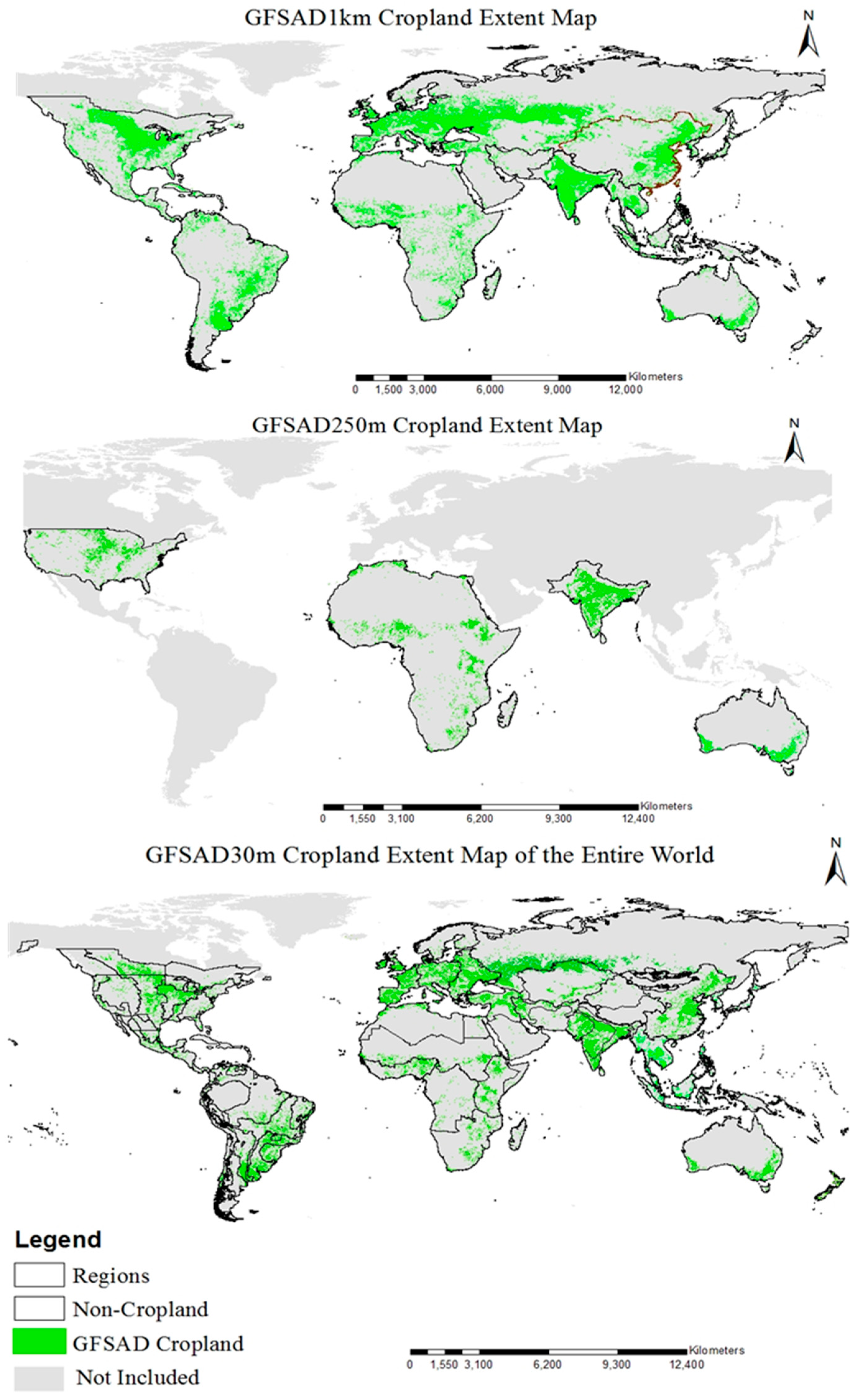
Recently, with the increased accessibility of advanced computing platforms for processing large datasets, an improved spatial and thematic dataset compared to previous cropland extent mapping efforts called the GFSAD Project (Global Food Security-support Analysis Data) was completed. Three new GFSAD cropland extent maps were created separately at three different spatial resolutions (1 km, 250 m, and 30 m) using Landsat and MODIS imagery, along with other existing cropland data for the nominal year 2015 [5,6,7,8,9,10,11,12,13,14,15,16,17,18]. These datasets are available for download through Data Pool, DAAC2Disk, and the NASA Earth Data Search. It is well known that mapping of cropland areas at different spatial resolutions can result in large differences in the estimates of cropland area and spatial extent [19,20]. Therefore, these three GFSAD cropland extent maps must be assessed and compared both at the global and regional scale to establish their quality and reliability as the base map for generating higher level cropland products such as crop type and crop intensity maps [21]. These maps provide for both large area (i.e., global) comparisons between the different spatial resolutions including the identification of similarities and differences and for determining their suitability for more regional analysis, especially when considering different agriculture field sizes [19]. Therefore, these three GFSAD cropland extent maps should be assessed and compared to explore the agriculture field sizes.
Previous attempts at rigorous accuracy assessment of large area cropland extent maps has been very limited. Considerable ambiguity exists in the implementation and interpretation of large area thematic map accuracy assessment. In the literature, individual measures and guidelines for assessing thematic map accuracy have been well established by many researchers [22,23,24,25]. However, these guidelines are not often followed due to various limitations in the assessment process (e.g., thematic resolution, geo-location accuracy and availability of reference data) [26]. The biggest limitation in the large area accuracy assessment process is the availability of valid reference data. As such, large area assessment efforts have mostly relied on insufficient, sparsely distributed reference data [27,28,29,30,31]. The assessments performed with limited and insufficient reference dataset reported overall accuracies ranging from 66% to 78%, with considerably lower accuracies of between 10% and 50% for the cropland class [32,33].
Cropland reference data are extremely limited in most parts of the world, resulting in insufficient sample sizes, and thus in an inability to assess the accuracy of large area thematic maps [34,35,36,37]. Recently, a few global reference datasets (e.g., FAO-GFRA (Food and Agriculture Organization Global Forest Resources Assessments) and the Geo-wiki sample set) have been developed to perform the assessment of global land cover maps [28,38]. Despite the increasing number of initiatives to collect reference datasets freely in the public domain such as Geowiki and GOFC-GOLD (Global Observation of Forest and Land Cover Dynamics), cropland reference datasets are still lacking. More work must be done to create additional global cropland reference datasets. Any new cropland reference dataset must be generated using an appropriate sampling design based on the inclusion probability of occurrence of crop and no-crop areas to assess these cropland extent maps [39]. If the inclusion probabilities of crop and no-crop areas are ignored, a significant bias is likely to occur resulting in a non-proportional and insufficient number of samples. Unless the reference data represents the entire cropland distribution, accuracy results will not be statistically valid and meaningful.
To perform the assessment on a global scale, the sampling design needs to be easy to implement and capable of accounting for the proportions of high and low map categories such as crop and no-crop distribution in different continents [40,41]. In simple random sampling, each sample of crop and no-crop class has an equal and independent chance of being selected [42]. However, such sampling designs might result in insufficient numbers of samples in the low crop proportion regions of different continents. Where possible (e.g., Landsat or Sentinel imagery), a homogeneous cluster of 3 × 3 pixels should be used as the sampling unit to account for the positional error at each location [42]. For coarser-resolution imagery (e.g., MODIS), it is difficult to find large homogeneous regions, and therefore, a single coarse-resolution pixel is used as the sample unit in these situations. The goal is to select the best sampling unit to ensure that only thematic error is considered in the accuracy measures and not error due to mis-registration or positional accuracy.
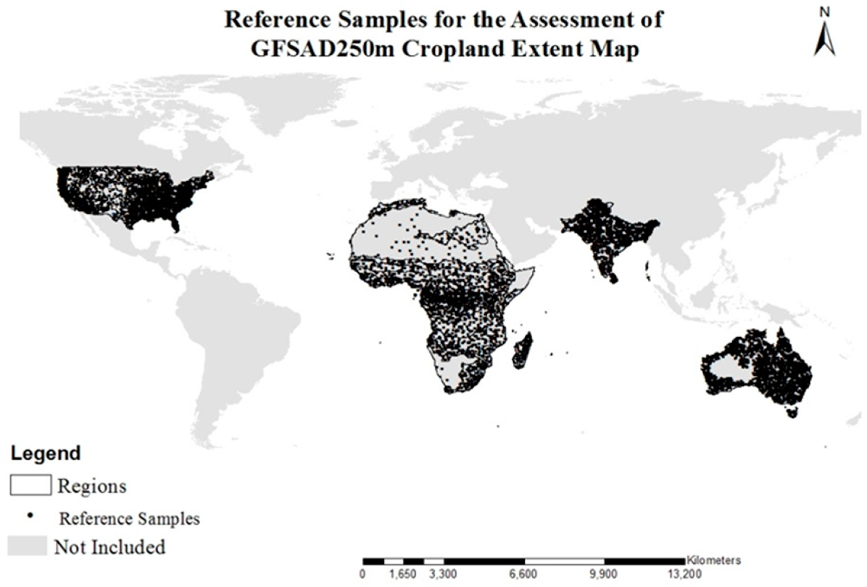
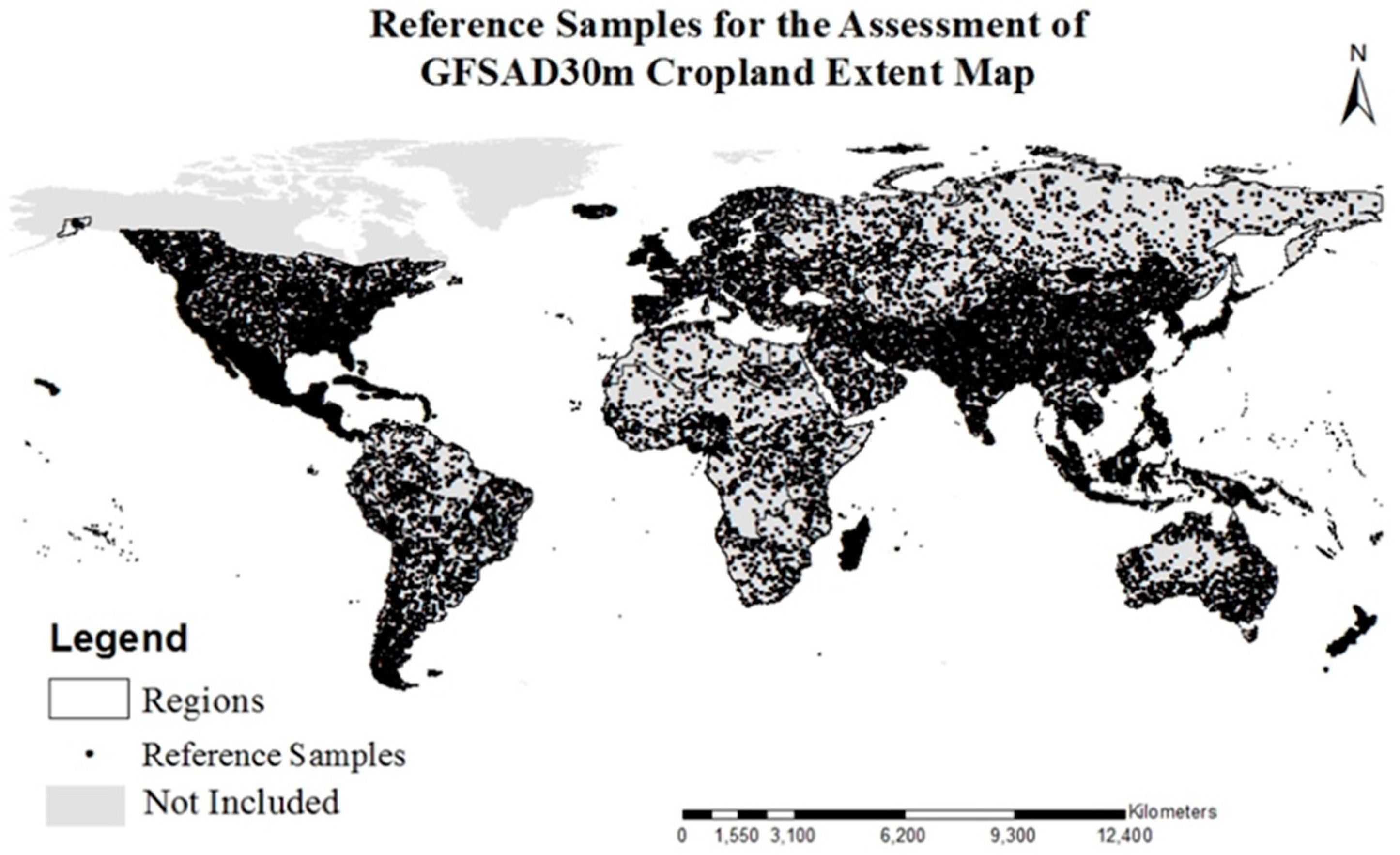
Another issue or limitation when conducting large area assessments is that most have reported just a single accuracy value for the entire world. This approach does not provide any details or information about the accuracy results for different continents or regions. Given the differences in crop growing strategies and patterns between continents, a more appropriate assessment strategy must be used. Such an assessment strategy has been recently used to assess the cropland extent maps of three different continents (i.e., the United States, Africa, and Australia) [43]. Yadav and Congalton [43] described an appropriate assessment strategy for these three continents based on their cropland distribution and reference data availability. This strategy employed a stratification approach to divide the entire world into homogeneous regions, and a sample simulation analysis was conducted to determine the appropriate sample size. Implementing a stratification approach prior to the actual assessment provided an effective means of evaluating the cropland extent maps by considering the diverse cropping patterns of different continents [37].
The most widely accepted approach for reporting thematic map accuracy results is using an error matrix [22,42]. The error matrix presents the comparison of reference samples with the map and allows computation of overall, producer’s, and user’s accuracy [44]. This assessment technique can be used to report these accuracy measures for different regions. In addition, there are some regions, such as the United States and Canada, where a reference cropland data layer (e.g., CDL in the US) exists for comparing the entire map on a pixel by pixel basis. Such comparison results can then also be presented in the form of a similarity analysis which represents the spatial distribution of agreement and disagreement that occurred in the map as compared to the reference map.
Finally, in addition to evaluating each of the three different GFSAD cropland extent maps separately, it is useful to perform a comparison between the maps to evaluate the effectiveness of each spatial resolution for specific user requirements [45,46]. Mapping at a variety of spatial resolutions raises many inconsistencies, differences, and uncertainties among the estimated cropland areas that can be visualized on the map and are the result of the spatial distribution of cropland patches in different cropping patterns [47,48]. Therefore, existing and newly developed cropland extent maps must be compared with each other to investigate, determine, and recommend the appropriate spatial resolution for agriculture monitoring given different agriculture field sizes and patterns. Many comparative studies have been performed for existing datasets such as GLC2000, MODIS, International Geosphere-Biosphere Program (IGBP), and National Land Cover Dataset (NLCD) [49,50]. Despite identifying spatial discrepancies and inconsistencies, particularly in the cropland class on a global scale, these comparison studies have not focused on the adequacy of different spatial resolutions given different agriculture field sizes [1,51]. The uncertainties in the cropland class of these existing maps could be due to: (1) absence of precise spatial location of the cropped areas; (2) coarse resolution of the map products, with significant uncertainties in areas, locations, and detail; and (3) invalid assessments of these cropland extent maps.
The recent production of the three different GFSAD cropland extent maps promises to provide more detailed and accurate cropland information with a high amount of certainty in the geographic location of the cropland areas. Therefore, these three different cropland extent maps must be assessed with an appropriate large area accuracy assessment strategy describing their use, reliability, and quality for different continents. However, cropland extent mapping in different agriculture fields sizes can be inconsistent at different spatial resolutions because of the spectral similarity of different fields and differences in similar agriculture fields [52]. The similarities and differences in the characteristics of agriculture landscapes (i.e., crop area proportions and landscape metrics) must also be explored to provide specific recommendations for when to apply the three different cropland extent maps with respect to different field sizes [53]. This kind of regional comparison can be effectively implemented by using a similarity matrix based on a contingency table approach like an error matrix and by categorizing landscape metrics such as landscape proportion for different agriculture field sizes.
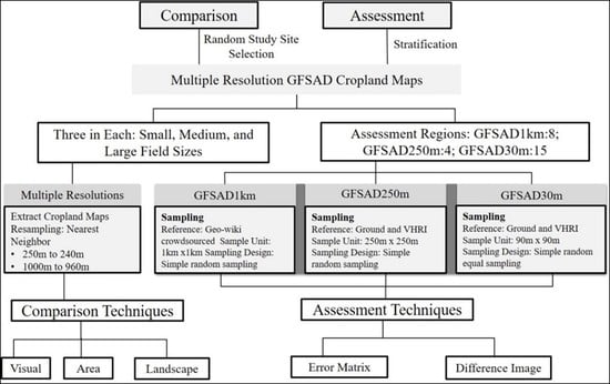
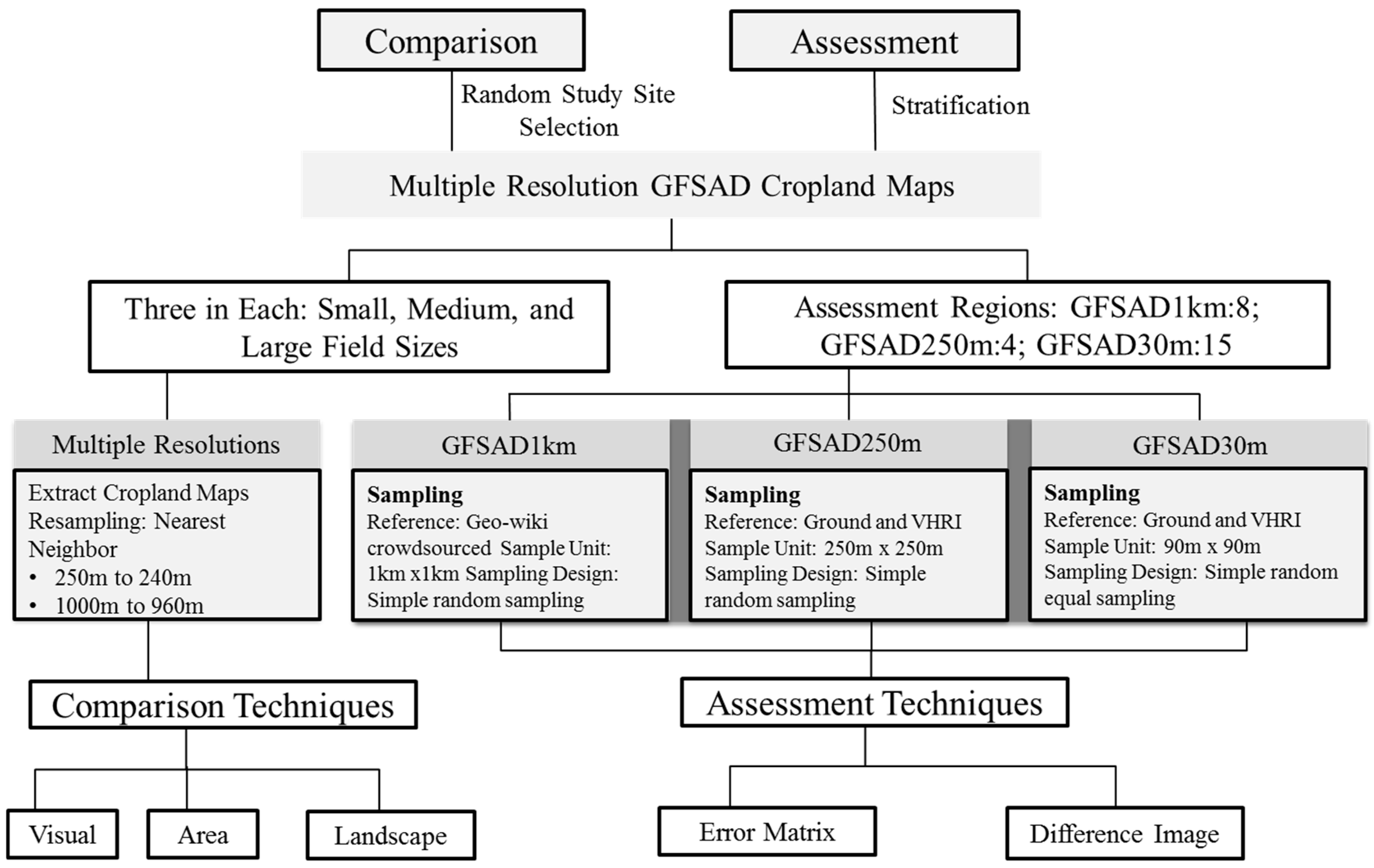
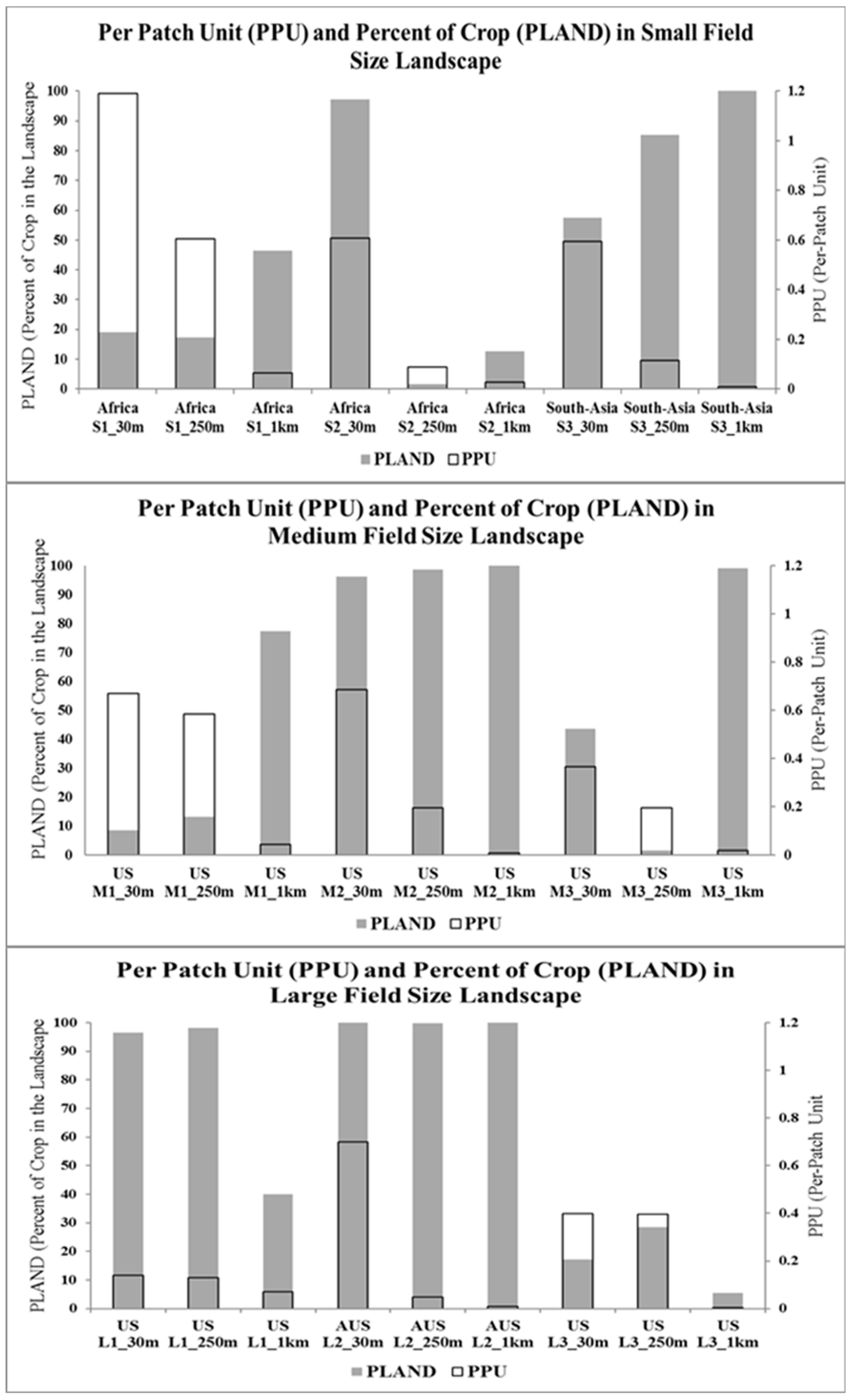
Therefore, the two primary objectives of this study are to perform an accuracy assessment of the three different GFSAD cropland extent maps of the world and then evaluate the impact of different agriculture field sizes on global and regional agriculture monitoring. To accomplish the first objective, a large area accuracy assessment was conducted separately for each spatial resolution GFSAD cropland extent map. Three different assessments were performed using a valid large reference data set collected from different sources and sampling simulations to choose the appropriate sample size for each region [
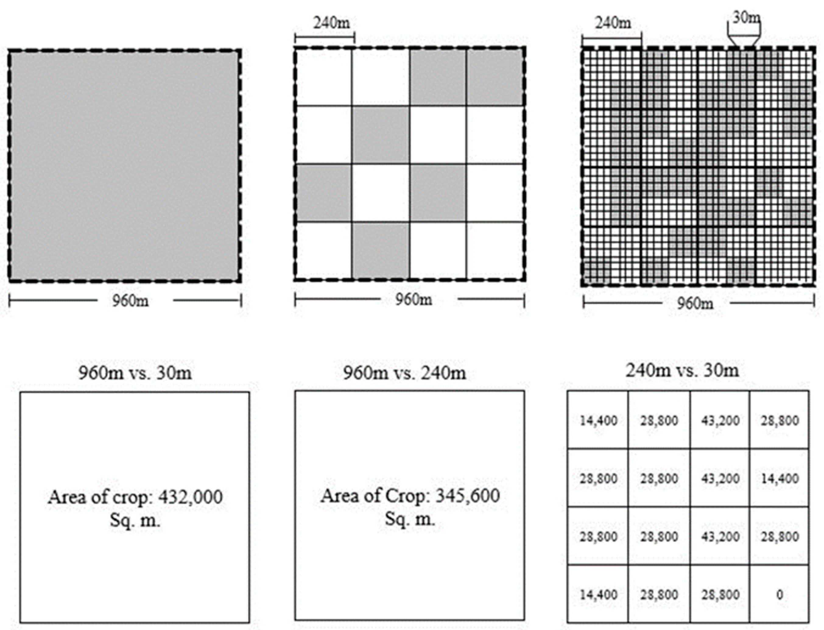
42,43]. Second, regional comparisons of the three GFSAD cropland extent maps were performed by calculating similarity in crop area proportions and landscape heterogeneity in nine random 10 km by 10 km study sites or regions selected in each of three agriculture field sizes (i.e., small, medium, and large). The specific goal of this paper is to provide an appropriate assessment and comparison of three different GFSAD cropland extent maps to resolve many of the short-comings and uncertainties of other cropland extent mapping efforts. Finally, the results of this analysis are used to recommend when it is appropriate to apply each map given the different agriculture field sizes for each continent of the world.

2. Materials and Methods

This section provides a description of the materials and the methods used to assess and compare the three different GFSAD maps. It consists of the following sub-sections: (1) Study area, (2) Datasets, and (3) Methodology.

2.1. Study Area

Two different study areas were used in this investigation. These are: (1) the entire world divided into eight, four, and fifteen zones to perform the assessment of GFSAD 1 km, 250 m, and 30 m cropland datasets, respectively; and (2) nine random 10 km by 10 km analysis areas used to perform the comparison of GFSAD maps by field size.
To perform the comparison, the agriculture field sizes of the entire world were grouped into three classes using a global field size map from International Institute for Applied Systems Analysis and International Food Policy Research Institute (IIASA-IFPRI). This map classified global field sizes ranging from 10 to 40 hectares (ha) at 1 km spatial resolution based on data collected via a Geo-Wiki crowdsourcing campaign [3]. The three classes of agriculture field size used in the study were: 10–20 ha (small), 20–30 ha (medium), and 30–40 ha (large). Nine study sites were randomly selected, with three in each agriculture field size across the entire world (Figure 1). Table 1 shows the distribution of selected study sites in different continents and agriculture field sizes.

2.2. Datasets

Four datasets were necessary to conduct the accuracy assessment of the GFSAD cropland extent maps. The first three datasets were the maps themselves at the three spatial resolutions (Figure 2), and the fourth was the reference data set used for comparison. The basic requirements and techniques to perform the thematic map assessment have been reviewed by many researchers in the past [22,24,42]. One of the key elements of the assessment is to ensure that the same appropriate classification scheme was used for collecting both the training data and the reference data. A well-defined classification scheme helps to reduce the risk of misunderstanding and inconsistencies while comparing and assessing the mapping products [42,54]. Therefore, a common GFSAD classification scheme was used to generate the three GFSAD cropland extent maps at different spatial resolutions and to collect the reference dataset used to validate these cropland extent maps. This classification scheme defines the cropland class as “lands cultivated with plants, harvested for food, feed, and fiber, including both seasonal crops (e.g., wheat, rice, corn, soybeans, and cotton) and continuous plantations (e.g., coffee, tea, rubber, cocoa, and oil palms)”. The fallow croplands are defined as “lands uncultivated during a season or a year but are farmlands and are equipped for cultivation, including plantations (e.g., orchards, vineyards, coffee, tea, rubber) [5]. The cropland extent maps include all the planted crops and fallow lands. Non-croplands include all land cover classes other than croplands and cropland fallow.
Accuracy assessment was conducted on the three cropland extent maps (GFSAD1km, GFSAD250m, and GFSAD30m). These maps were produced for the entire world with the exception of the GFSAD250m cropland extent map, which is only available for four of the continents. These cropland extent maps are listed in Table 2, describing their mapping year, spatial resolution, input data, assessment regions, and classification scheme.
The GFSAD1km cropland extent map was derived as a disaggregated five class global cropland extent map at nominal 1 km resolution using four existing multi-study crop mask layers [4,31,55]. Two of the five classes are dominated by irrigated and rain-fed agriculture. The other three classes have minor/very minor fractions of croplands. The irrigation minor class represents the areas irrigated by small reservoirs, irrigation tanks, open wells, and other minor irrigation. The GFSAD1km cropland extent map is available online with these five irrigated and rainfed classes, was downloaded, and a cross-walk was developed to simplify the five classes into a crop/no-crop class map for assessment and comparison with other GFSAD cropland extent maps (Figure 2).
The GFSAD250m was developed at a spatial resolution of 250 m using MODIS satellite data for only selected regions of the world (the United States (US), Australia, Africa, and South-Asia as shown in Figure 2). The cropland extent maps of each selected region were developed by different mapping teams as a part of the GFSAD project [5,6,7,8,9,10,11,12,13,14,15,16,17,18].
The GFSAD30m cropland extent map was developed at a spatial resolution of 30 m for 6 continents using multi-temporal Landsat satellite imagery [9,10,11,12,13,14,15,16,17,18]. This cropland extent map was generated for the nominal year 2014 using an automated classification algorithm (i.e., random forest classifier) on the cloud-computing Google Earth Engine (GEE) platform. Figure 2 shows the cropland areas mapped in the GFSAD30m cropland extent map for the entire world.
In addition to the three different GFSAD cropland extent maps, the fourth and final dataset used in this study is the global reference dataset collected at the same three spatial resolutions from various sources to perform the accuracy assessment. These different sources of reference data include existing reference samples and maps (e.g., crowd-sourced Geo-wiki data and USDA Cropland Data Layer), ground-collected data, very high-resolution image (VHRI) interpreted reference samples collected by a GFSAD team member stored on the cropland.org database, and an independently generated reference data by the accuracy assessment team (Table 3).
One of the existing reference data sources is IIASA’s Geo-wiki reference data, which is a global, but sparsely distributed, crowd-sourced dataset usually collected by experts using high-resolution images [18,20]. Geo-wiki reference data consists of varying size polygons located across the entire world and a legend showing the percentage of cropland in each sample [56]. The reference samples were evaluated by IIASA experts using high-resolution images through the Geo-wiki crowdsourcing land cover validation tool [28]. This dataset has been proven to be valuable in accuracy assessment of 1 km mapping products [28,57]. Both crop and no-crop reference samples selected in our work were 1 km by 1 km homogeneous polygons which were reviewed, re-interpreted, and used to assess the GFSAD1km cropland extent map for the year 2010.
A second existing reference source is high-quality reference cropland extent maps such as the USDA Cropland Data Layer (CDL) and the Agriculture and Agri-Food Canada (AAFC) cropland layers. The National Agricultural Statistics Service (NASS) of the United States Department of Agriculture (USDA) developed the CDL product for the entire United States [58]. The CDL product is a comprehensive, raster-formatted, geo-referenced, and crop-specific land cover map that utilizes ortho-rectified imagery to identify field crop types accurately and geospatially. Similarly, the AAFC Annual Space-Based Crop Inventory for Canada provides information at 30 m spatial resolution for the location, extent and changes in Canadian crops [59]. Since 2011, AAFC has consistently delivered an annual crop inventory for all the Canadian provinces. These existing data sources provide annual and continuous cropland information at a high spatial resolution.
To supplement existing maps and sample datasets, new reference data on croplands were also generated from: (1) the field campaigns conducted by the GFSAD mapping teams [6,11,14] and (2) the interpretation of high-resolution imagery (HRI) by the team members of the GFSAD project. These field campaigns provided reference data not only on crop extent (cropland vs. no-cropland), but also on crop type, irrigated vs. rain-fed, and crop intensity (single, double crop per year). For example, campaigns were conducted for Australia and South-East Asia in the years 2014 and 2015, respectively.
Most of the new reference data was obtained by interpretation of HRI. Two collection efforts were employed. First, one GFSAD project team member interpreted a great deal of HRI imagery of multiple years and sub-meter spatial resolution for use by the entire GFSAD team. These interpreted samples were split 60/40 with 60 percent of the data being used by the mapping teams for training and testing of their classification algorithms. Forty percent was set aside and hidden from the mapping teams and used in the process of accuracy assessment. The accuracy assessment team used this 40 percent of the reference data, but only after reviewing each sample and confirming the interpretation. If both interpreters agreed, then the sample was selected for use. Second, a supplemental independent set of reference samples was generated by visual interpretation of Google Earth imagery solely by the accuracy assessment team. Again, here, two interpreters were used to ensure high accuracy in the reference data. These samples were collected for many low-cropland regions (e.g., Australia and Africa) to either supplement the low sample size or to achieve a proportional reference data size necessary to perform a valid accuracy assessment of the three different GFSAD cropland extent maps.

2.3. Methodology

The objectives of this study were accomplished using two main methods: (1) thematic map accuracy assessment and (2) map comparison. First, to perform large area thematic accuracy assessment of the three GFSAD cropland extent maps, an assessment strategy was employed based on the availability of reference data, cropland distribution, and mapping strategies used for each continent [43]. Second, the comparison of GFSAD cropland extent maps was performed on randomly selected analysis areas of 10 km by 10 km in the three different agriculture field sizes. The overall methodology (Figure 3) that was followed to assess and compare the three different GFSAD cropland extent maps is described in the following two sub-sections:

2.3.1. Assessment

The accuracy assessment of the three GFSAD cropland extent maps was executed in the following steps: (1) Stratification, (2) Sampling, and (3) Assessment Technique. An appropriate assessment strategy was used, employing a stratification approach to divide the entire world into homogeneous regions followed by a sampling design derived from the results of a sampling simulation analysis.
First, the process of dividing an area into homogeneous regions based on some relevant factor is referred to as stratification. This relevant factor could be either an administrative or ecological parameter or a combination of both to provide a more meaningful and useful assessment. The stratification of the three different cropland extent maps into homogeneous regions in this study was based on one of the following three different criteria: (1) Agro-Ecological Zones (AEZs) provided by FAO, (2) a buffer approach, or (3) AEZs combined with country boundaries. Agro-Ecological Zones (AEZs) are created based on the length of the growing period days of crops in homogenous climatic and topographic conditions or regions [60]. Because it was difficult to stratify areas using the AEZ approach in some parts of the world due to the very low proportion of cropland, a more effective stratification method (i.e., buffering approach) was used to define an appropriate sampling area around these cropland patches instead (e.g., Australia, Alaska, Iceland, and Mongolia) [43]. Finally, in some areas, the AEZ approach was combined with country boundaries to stratify the area into a more reasonable number of regions.
The three cropland extent maps were stratified specifically according to their mapping strategy, reference data availability, and the spatial resolution. For example, the GFSAD1km cropland extent map was assessed using 8 regions based on the availability of a proportional and optimum size of reference data available from IIASA’s Geo-wiki. Similarly, the GFSAD250m cropland extent map was assessed using 4 regions mapped simply as the four different continents. Finally, the GFSAD30m cropland extent map was assessed using 15 regions which were combined with country boundaries from the original 72 AEZ-based homogeneous regions (Table 4).
Second, an appropriate sampling approach is comprised of a sampling scheme, a sample unit, and a sample size (i.e., appropriate number of samples) for collecting valid reference data. The sampling design needs to be easy to implement and capable of accounting for the proportion of high and low map categories such as crop and no-crop distribution in different continents in order to perform the assessment on a global scale [41]. A simple random sampling scheme was employed for each region to collect a sample proportional to the cropland and non-cropland extent map class distribution. A sample unit of 90 m × 90 m was used to collect reference samples to assess the GFSAD30m cropland extent map. In contrast, sample units of 250 m × 250 m and 1 km × 1 km were used to assess the GFSAD250m and GFSAD1km cropland extent maps, respectively. The most challenging component of sampling is the collection of a sufficient number of samples. The number of samples to assess the GFSAD1km cropland extent map was determined based on the availability of Geo-wiki samples and the proportional area of the different regions. After a thorough review of Geo-Wiki dataset, it was observed that all the eight regions could be sampled with a minimum sample size of 200. This minimum sample size was balanced with the area proportions in each region. To assess the GFSAD250m and GFSAD30m cropland extent maps an optimum sample size of 250 was selected based on a Monte Carlo sampling simulation analysis.
Third, the accuracy of the three different GFSAD cropland extent maps was evaluated using two different assessment techniques: (1) an error matrix and (2) a difference image. First, error matrices were generated by comparing the map and reference labels using a program written in R. The error matrix was then used to calculate various measures of accuracy including overall, producer’s, and user’s accuracies [22,44]. Second, a difference image was generated by comparing the GFSAD250m and GFSAD30m cropland extent map for the United States with the resampled and cross-walked CDL reference map. This analysis was possible only for the US because of the availability of this CDL reference map. The two difference images generated at two different spatial resolutions clearly demonstrated the spatial distribution of agreement and disagreement between these two thematic maps.

2.3.2. Comparison

The three different cropland extent maps were compared for the three different agriculture field sizes based on the following three characteristics observed at the three different spatial resolutions: (1) the look of the map, (2) cropland area similarity, and (3) heterogeneity or clumping in the cropland landscape. First, the look of the spatial extent of the cropland patches at three different spatial resolutions was compared with the expected cropland distribution from high-resolution reference images to show how the map looks at each resolution. This method is simply a qualitative comparison. Second, the similarity of cropland areas mapped at different spatial resolutions was determined based on a contingency table approach in the form of a similarity matrix [61]. The area of each mapped class of the fine resolution cropland extent map was presented in the rows while the area of each class on the coarse resolution map was presented in the columns of the similarity matrix (Table 5).
In Table 4, A11 and A22 denote the area that is classified as Class 1 and Class 2, respectively, both in the fine- and coarse-resolution cropland extent maps. The diagonal values represent the consistency or the similarity for each class between the fine and coarse resolution maps. The column totals A+1 and A+2 sums the area of class 1 and class 2 on the coarse resolution map, respectively. Likewise, A1+ and A2+ represent the row totals of Class 1 and Class 2, respectively, on the fine-resolution cropland extent map. The commission error (CE) for class i can be evaluated by A + i A i i A + i , which represents the percentage of area for class i that is committed from the fine-resolution map. The omission error (OE) for class i in the coarse map can be evaluated by A i + A i i A i + , which represents the percentage of area for class i that is omitted from the coarse map. The overall similarity (OS) was evaluated by i = 0 n A i i i = 0 n A i + = i = 0 n A i i i = 0 n A + i , which represents the percentage of the area for all classes that are correctly represented in the coarse-resolution map. The calculation of the similarity matrix for crop and no-crop classes was performed in the following seven steps:
  • The area comparison was initialized with a resampling of 250 m to 240 m map and 1 km to 960 m map, respectively, making all three cropland extent maps comparable with each other. This resampling was necessary to incorporate the 30 m spatial resolution map.
  • Compute the total number of the square windows (NSW) of the coarse-resolution map required to cover the fine-resolution map.
  • Place the square window over the fine-resolution map. The value of the square window corresponds to the class label of the coarse-resolution map.
  • Identification of class label of coarse- and fine-resolution map pixels within the square windows.
  • Calculate the area of class 1 and class 2 of the fine-resolution map within the coarse pixel.
  • This comparison was performed by moving a 240 m and 960 m window over different-resolution cropland extent maps (Figure 4). Within the moving window, the high-resolution cropland extent map area was calculated. In Figure 4, each moving coarse-resolution square window represents the area of cropland calculated from high-resolution cropland pixels.
  • Finally, all the comparisons were reported as a tabular array i.e., a similarity matrix comparing the two pairs of cropland extent maps [61].
All the above-mentioned comparison steps were implemented on three pairs of combinations (i.e., 960 m–30 m, 960 m–240 m, and 240 m–30 m) for calculating the cropland area mapped at fine spatial resolution within the coarse-resolution pixels at nine study sites with different agriculture field sizes (Figure 4).
Third, two landscape metrics, Per-Patch-Unit (PPU) and the Percentage of LANDscape (PLAND), were calculated and compared for each study site to understand the heterogeneity and clumping in the cropland landscape at three different resolutions with respect to different agriculture field sizes [42]. The most common landscape clumping metric, contagion, was replaced with an alternative, more suitable landscape metric, PPU, because it is less sensitive to spatial resolution and more sensitive to landscape pattern. The PPU values are expected to be low for less fragmented landscapes and increase with landscape fragmentation. The PPU metric was calculated by using PPU=m∕(nxλ) for each study site, where m is the total number of patches, n is the total number of pixels, λ is a scaling constant equal to the area of a pixel and expressed in sq. m. units. In addition to PPU, the PLAND metric was calculated in Fragstats software for each study site to measure landscape composition (i.e., how much of the landscape is comprised of a patch type (e.g., cropland)). The PPU (clumping or fragmentation levels) and PLAND (the percentage of landscape in cropland) were compared by plotting their values for different agriculture field sizes to understand and analyze the discrepancies and similarities among the three different cropland extent maps. Finally, based on the comparison results, more specific insights, suggestions, and recommendations were provided for when to apply the three different GFSAD cropland extent maps considering different agriculture field sizes.

3. Results

The accuracy assessment of the three different cropland extent maps follow an appropriate assessment strategy implemented in three main steps: (1) stratification, (2) sampling, and (3) accuracy. The first three sub-sections present the accuracy results for three different cropland extent maps performed in a similar fashion. The fourth subsection presents the comparison of the three cropland extent maps.

3.1. GFSAD1km Assessment

The accuracy assessment of GFSAD1km cropland extent map was performed in eight regions using 1800 crop and no-crop samples as shown in Figure 5. Table 6 presents the area of each region, the area proportion of each region, and the number of reference samples used for each. Table 7 reports the overall, producer’s, and user’s accuracy of GFSAD1km map achieved by region, while Table 8 is the summary error matrix for the entire world. The regional overall accuracies range from 73.3% to 85.2%. The overall accuracy of GFSAD1km cropland extent map is 78.7% with a low (59.3%) user’s accuracy of crop.

3.2. GFSAD250m Assessment

The results of the accuracy assessment of GFSAD250m cropland extent map performed in four regions using a reference dataset of 7762 samples includes overall, producer’s, and user’s accuracy reported in the form of an error matrix (Figure 6, Table 9). The user’s accuracy of crop in Africa is slightly less than other regions (64.6%). The overall error matrix and the overall accuracy of the four regions combined (94.8%) are presented in Table 10.

3.3. GFSAD30m Assessment

The accuracy assessment of GFSAD30m cropland was map performed in 15 regions using a reference dataset of 19,171 samples as shown in Figure 7. Table 11 shows the total number of regions, their area, and the reference samples selected for each of the 15 combined regions. The accuracy results of GFSAD30m cropland extent map are presented in an error matrix for the entire world and a difference image, just for the US. First, the overall, producer’s, and user’s accuracy were calculated for all the 15 regions and presented in Table 12, along with total number of samples. Most of the regions have high overall accuracy ranging from 84.5% for South-Asia to 98.3% for Mongolia. The overall error matrix and the overall accuracy of GFSAD30m cropland extent map for the entire world (91.7%) are presented in Table 13.
In addition to the error matrix, the disagreement in the cropland areas mapped in the GFSAD250m and GFSAD30m cropland extent maps are presented in the form of difference images for the US. Creation of the difference images is possible because of the availability of a complete reference map (i.e., CDL). Figure 8A,B shows the spatial distribution of agreement and disagreement in the cropland areas mapped in the GFSAD250m and GFSAD30m, as compared to the reference, cropland extent maps. The GFSAD250m cropland extent map has only 2% omission error and no commission error in the cropland areas as compared to resampled CDL 250m reference map. The GFSAD30m cropland extent map has 7% omission and 8% commission error in the cropland areas as compared to CDL 30 m map. In other words, the GFSAD30m cropland extent map is 85%, similar to the CDL 30 m reference map.

3.4. Comparison of the Three Different GFSAD Cropland Extent Maps

Figure 9 presents a visual comparison of the GFSAD1km, GFSAD250m, and GFSAD30m cropland extent maps with the high spatial-resolution imagery at nine random study sites for three different field sizes. All three cropland extent maps look similar to each other for the large agriculture field sizes of the US and Australia. The GFSAD250m and GFSAD30m cropland extent maps look more similar to each other than the GFSAD1km cropland extent map for the medium field sizes of the US and the small agriculture field sizes of South-Asia and Africa. Finally, the visual comparison shows that the cropland areas mapped in the GFSAD30m cropland extent map look more similar to the spatial extent of the agriculture fields as seen on the high-resolution imagery acquired for the same mapping year.
Second, the area comparison performed using the similarity matrix approach shows the overall similarity between the three different cropland extent maps with respect to different agriculture field sizes (Table 14, Figure 10). All three cropland extent maps (i.e., GFSAD30m, GFSAD250m, and GFSAD1km) have high similarity in their cropland areas with respect to the large agriculture field sizes of the US and Australia and the small field sizes of South-Asia. However, the GFSAD1km cropland extent map has low similarity with the other two cropland extent maps (i.e., GFSAD30m and GFSAD250m) with respect to medium and small field sizes for each continent.
In addition to the overall similarity, the similarity matrix approach made it possible to identify omission and commission errors introduced into the cropland areas mapped at coarse spatial resolution through comparison with the fine spatial resolution images. The estimated errors of each study site are represented as the percent of cropland areas which were either omitted from or committed to the coarse-resolution cropland extent maps (Table 15). For each study site, three different omission (OE) and commission errors (CE) were calculated, one for each of the three combinations of coarse- and fine-resolution cropland extent maps. For example, the omission error presented in the third column of Table 15 (i.e., 58.0%) represents the percentage of cropland areas omitted from the 250 m map as compared to the 30 m map in the small agriculture fields of Africa. The additional rows in the third column (i.e., 82.3% and 82.7%) represents the omission in the cropland areas from the 1 km map when compared to 30 m and 250 m cropland extent maps, respectively.
Third, the comparison of two landscape metrics (i.e., PLAND and PPU) calculated for each study site shows the similarity between the three different GFSAD cropland extent maps for the three different agriculture field sizes and spatial resolutions (Table 16). Figure 11 and Figure 12 show the values of PLAND and PPU, respectively, as calculated for the three different spatial resolution maps for the three different agriculture field sizes. Figure 13 presents the comparison of the two landscape metrics separately in each agriculture field size to clearly show the similarity among the three different cropland extent maps.

4. Discussion

With the release of three different resolution GFSAD cropland extent maps, it becomes crucial to know their individual accuracy and similarity to make a choice on using these maps in different agriculture field sizes [5,6,7,8,9,10,11,12,13,14,15,16,17,18]. This paper presented an appropriate accuracy assessment and detailed comparison of the three cropland extent maps at random study sites in different agriculture landscapes that are consistent with previous assessment and comparison studies [56]. Therefore, the assessment and comparison results must be discussed to provide insight into the quality, reliability, (un)certainty, and similarity of the GFSAD crop extent maps at different spatial resolutions of each region to determine the specific recommendations for their use in different agriculture field sizes [61,62].

4.1. Assessment of the Three Different GFSAD Cropland Extent Maps

The assessment of the three different cropland extent maps was performed using an accuracy assessment approach involving stratification and appropriate sampling resulting in accuracy measures for different regions of the entire world. The accuracy measures (e.g., overall, user’s, and producer’s accuracy) estimated for the entire world and within individual regions establish the quality of the three GFSAD cropland extent maps and how they vary by distribution and agricultural field size within each region. The overall accuracy results show that the GFSAD30m cropland extent map (91.7%) is more accurate than the coarse-resolution GFSAD1km map (78.7%). This result was expected, due to the more detailed mapping at a smaller pixel size (i.e., 30 m) that acts to remove the spectral mixing that is common with coarse resolution pixels (Table 8 and Table 13) [10]. However, the overall accuracy of the GFSAD250m crop extent map (94.8%) is unexpectedly higher than GFSAD30m map. However, this result is easily explained, as this assessment represents only four continents, and not the complexity of the entire world.
The overall accuracies of the three different cropland extent maps were also estimated for different regions in addition to their individual single overall accuracy of the entire world. The overall accuracy for individual regions of the GFSAD1km, GFSAD250m, and GFSAD30m cropland extent maps range from 73.3% to 85.2% in the eight regions, 80.7% to 98.2% in the four regions, and 84.5% to 94.7% in the fifteen regions, respectively (Table 7, Table 9 and Table 12). The reason for achieving different overall accuracies in different regions is related to cropland distribution, proportion, size of the agriculture fields, and cropping patterns of each region. However, the overall accuracies of the GFSAD30m cropland extent maps of each region are still higher than the coarse-resolution GFSAD250m and GSFAD1km maps. Therefore, the single overall accuracy of the three cropland extent maps estimated for each region and the entire world indicate that the high-resolution GFSAD30m cropland extent maps are more accurate than the coarse-resolution maps.
In addition to the single overall accuracy of the cropland extent maps that has been typically reported in the literature, the assessment of each region provides additional information, including crop extent user’s and producer’s accuracies. It has been shown in this study that the GFSAD1km crop extent user’s accuracy is lower (50.7%) than the GFSAD250m (64.6%) and GFSAD30m cropland extent maps (98.5%) in some regions (e.g., Africa) (Table 7, Table 9 and Table 12). These differences are due to the distribution, proportion, and size of the agriculture fields of each region. In contrast, the GFSAD250m crop extent map user’s and producer’s accuracies of the US, South-Asia, and Australia are higher when compared to Africa. While Australia also has a sparse distribution of cropland like Africa, the cropland distribution is more compact and concentrated toward the edges of the continent. Therefore, due to the differences in the cropland distribution and field size, Australia and Africa achieve different user’s accuracies for the GFSAD250m and GFSAD1km crop extent maps.
The accuracy measures estimated in Table 12 show that the GFSAD30m crop extent user’s accuracy ranges from 64.1% (Australia) to 100.0% (Iceland). The GFSAD30m crop extent map user’s accuracy of Africa (98.5%) indicates that the small size of agriculture fields of Africa when they occur in a heterogeneous cropping pattern can be accurately mapped at high spatial resolution. However, the GFSAD30m user’s accuracy of Australia is low because of the sparse cropland distribution and large agriculture field sizes. It can be seen from the assessment results of this paper that the low user’s accuracies of crop were mostly reported in the low crop proportion regions of the entire world, irrespective of the spatial resolution of the crop extent map. Therefore, it is important that a detailed analysis of the accuracy measures of low crop probability regions be performed in the future to achieve meaningful assessment results.
In addition to the crop extent user’s and producer’s accuracy, it is very important to know the spatial distribution of errors in the cropland areas at different resolutions to establish the quality of cropland extent maps for their efficient use at local or regional scales. The difference image generated based on a pixel-by-pixel comparison of the reference and classified cropland extent maps of the US presents the spatial distribution of the omission and commission errors introduced into the cropland regions at 250 m and 30 m spatial resolutions. The high spatial resolution crop extent map (i.e., GFSAD30m) has more omission and commission errors in the cropland areas than the coarser-resolution maps (Figure 8). The probability of errors occurring at high spatial resolution increases with an efficient identification of the edges of agriculture fields using an object-based classification approach and the removal of spectral mixing caused by the natural vegetation that is common in a coarse resolution pixel.

4.2. Comparison of the Three Different GFSAD Cropland Extent Maps

The comparison of the three different crop extent maps was performed to present the similarity among the three different cropland extent maps in three different agriculture field sizes of different continents (e.g., Australia, United States (US), South-Asia, and Africa) [19]. The similarity among the three crop extent maps were determined using the cropland landscape characteristics (e.g., look, area proportion, and clumping) mapped at different spatial resolutions and different size of agriculture fields (Figure 9, Figure 10, Figure 11 and Figure 12). First, the cropland distribution of the three crop extent maps was compared visually to decide how similar they look in different field sizes (Figure 9). As the spatial resolution of the cropland extent mapping increases, the look of the cropland distribution becomes more similar to the ground or other high-resolution imagery (e.g., Google Earth imagery) due to the removal of the spectral mixing from the surrounding pixels that is more common at larger pixels [52].
Second, the change in the area proportion of the cropland landscape was used to determine the similarity of the three crop extent maps by counting the number of overlapped crop pixels between the coarse- and fine-resolution map using a similarity matrix approach (Figure 10). The percent of cropland areas omitted and committed to the coarse-resolution cropland extent maps due to the change in the pixel size were estimated as omission and commission errors in different agriculture field sizes (Table 15) [53]. The quantification of the changes in the cropland area proportions in the form of overall similarity, omission, and commission errors at different resolutions and field sizes are important in determining the similarity among the three different crop extent maps (Figure 11). Third, the clumping of the cropland patches (i.e., PPU) characteristic of the cropland landscape also experiences changes at different spatial resolutions and field sizes due to fragmentation of the large cropland patches at a smaller pixel size. The clumping of the cropland areas (i.e., PPU) decreases with increasing spatial resolution, as the landscape becomes more generalized and aggregated from high-resolution to low-resolution cropland extent maps (Figure 12) [53]. Therefore, the variations observed in the look, area proportion, and clumping of the cropland landscape are very crucial for determining the similarity among the three crop extent maps in different agriculture field sizes.
The similarity of PLAND and PPU at different spatial resolutions and field sizes demonstrates that all three crop extent maps have equal similarity in the large field sizes of Australia, the medium and large field sizes of the US, and the small field sizes of South-Asia (Figure 10, Figure 11 and Figure 12). However, the high-resolution crop extent maps (i.e., GFSAD30m) are more similar to the 250 m map than the 1 km crop extent maps for the small field size of Africa and the medium field size of the US (Table 14) due to their cropland distribution. As a result, the similarity in the characteristics of cropland areas mapped at different spatial resolutions provides suitable considerations and recommendations for using the three different crop extent maps in different agriculture field sizes (Figure 11 and Figure 12). Based on the comparison results of this paper, it can be clearly stated that agriculture monitoring must be carefully performed in different agriculture field sizes on different continents of the world (e.g., Africa, South-Asia, Australia, and the US) using an appropriate spatial resolution crop extent map.

4.3. Determining Specific Recommendations for When to Apply the Three GFSAD Cropland Extent Maps

With the availability of three different GFSAD cropland extent maps, the question of choosing an appropriate and suitable map for carrying out agriculture monitoring and management practices on different agriculture field sizes becomes a viable consideration. The comparison of the three different GFSAD cropland extent maps performed in this paper can be used to provide suitable recommendations for when to apply these maps in different agriculture field sizes (Figure 13). The comparison of the characteristics of the cropland landscape indicate high similarity among the three different cropland extent maps in the large agriculture fields of the US and Australia and in the small fields of South-Asia. However, the cropland characteristics (i.e., look, area, and clumping) of the GFSAD30m and GFSAD250m crop extent maps are more similar than the GFSAD1km map in the medium and small field sizes of the US and Africa. Based on the low and high similarity of the proportion (PLAND) and clumping of cropland landscape (PPU) among the three cropland extent maps, recommendations for when to use which maps at the appropriate and suitable spatial resolution in different field sizes were developed. Table 17 presents these recommendations, which can be used for different field sizes on each of the continents to perform agriculture monitoring.

5. Conclusions

Over the last few years, the mapping of global cropland datasets has been rapidly increasing. With the recent release of the three different GFSAD cropland extent maps produced by different researchers, their quality and reliability must be evaluated at global and regional scales. Previous assessments of global thematic maps have been limited by the small size of the reference data used resulting in reporting a single global accuracy value for the entire world. The large area accuracy assessment of three different GFSAD cropland extent maps performed here demonstrates an appropriate sampling strategy for collecting a large cropland reference dataset necessary to achieve meaningful accuracy results not only for the entire world, but also by continent. The assessment report of GFSAD30m cropland extent map is available at https://lpdaac.usgs.gov [63].
When a global cropland extent map needs to be assessed for individual continents, the prevalent cropland distribution, area, spatial extent, and pattern of each region are very important to be considered for providing meaningful accuracy measures. Accuracy assessment performed in regions with varying crop proportion regions showed that a statistically valid, proportional, and random sampling design resulted in an insufficient sample size and low accuracy measures for regions with low cropland distribution and proportion. Therefore, depending on the objective of assessing the crop and no-crop maps of these low crop proportion regions, alternative sampling designs should be employed to achieve meaningful accuracy measures.
In addition to the estimation of accuracy measures of different continents, the overall accuracy of the three different cropland extent maps of the entire world show that the cropland extent mapping becomes more accurate towards the higher spatial resolutions. Consequently, the GFSAD30m cropland extent map with higher overall accuracy would be potentially preferable to the other coarser-resolution maps. However, despite the differences in the overall accuracy of the three different cropland extent maps, different-resolution cropland extent maps need to be compared in order to provide recommendations as to when to apply which map in different agriculture field sizes. The comparison of the characteristics of the cropland landscape mapped at the three different spatial resolutions is a very effective way of establishing the similarity among the cropland extent maps. The similarities between the three cropland extent maps were used to develop the following three main recommendations for the farmers, crop yield predictors, food market researchers, and policy- or decision-makers in choosing a suitable cropland extent map for agriculture monitoring in different agriculture field sizes:
  • The cropland extent maps developed at 30 m spatial resolution must be used in small agriculture field sizes of Africa. However, the cropland extent maps developed at 30 m and 250 m spatial resolution can be used for agriculture monitoring in small agriculture fields of South-Asia.
  • The cropland extent maps developed at either 30 m or 250 m spatial resolutions are recommended for the medium field sizes of the United States for different agriculture monitoring purposes.
  • The cropland extent maps developed at 30 m, 250 m, and 1 km spatial resolutions (i.e., any of the different spatial resolution crop extent maps) can be used in the large agriculture field size of Australia and the United States.

Author Contributions

R.G.C. and K.Y. conceived the idea for this paper. The cropland extent maps for different continents were developed and provided by NAU, UW, and USGS team as a part of GFSAD project. The compilation of cropland extent maps and the data analysis was done by K.Y. The reference data to perform the assessment were collected by P.T., Mr. B.S., and K.Y. Tables and figures that resulted from the assessment were generated by K.Y. along with the first draft of the writing. The final paper was edited by R.G.C. and K.Y. The final edits were compiled by K.Y. who converted the paper to the final format for this journal.

Funding

The research is funded by NASA MEaSUREs (Making Earth System Data Records for Use in Research Environments). The United States Geological Survey (USGS) provided supplemental funding as well as numerous other direct and indirect support through its Land Change Science (LCS), Land Remote Sensing (LRS) programs, and Climate and Land Use Change Mission Area. The NASA MEaSUREs project grant number: NNH13AV82I, the USGS Sales Order number: 29039. Partial funding was provided by the New Hampshire Agricultural Experiment Station. This is Scientific Contribution Number 2795. This work was supported by the USDA National Institute of Food and Agriculture McIntire Stennis Project #NH00077-M (Accession #1002519).

Acknowledgments

We would like to thank the entire GFSAD team, under the leadership of Prasad Thenkabail, for providing the cropland extent maps of the different continents used to perform the assessment and comparison at three different spatial resolution.

Conflicts of Interest

The authors declare no conflict of interest.

References

  1. Gong, P.; Clinton, N.; Yu, L.; Liang, L. The 30 m global land cover products from China: progress and perspectives. In Proceedings of the International Symposium on Land Cover Mapping for the African Continent, Nairobi, Kenya, 25–27 June 2013. [Google Scholar]
  2. Atzberger, C.; Vuolo, F.; Klisch, A.; Rembold, F.; Meroni, M.; Mello, M.P.; Formaggio, A. Land Resources Monitoring, Modeling, and Mapping with Remote Sensing, 2015th ed.; Thenkabail, P.S., Ed.; CRC Press-Taylor and Francis Group: Boca Raton, 2015; ISBN 1482217988. [Google Scholar]
  3. Fritz, S.; See, L.; McCallum, I.; You, L.; Bun, A.; Moltchanova, E.; Duerauer, M.; Albrecht, F.; Schill, C.; Perger, C.; et al. Mapping global cropland and field size. Glob. Chang. Biol. 2015, 21, 1980–1992. [Google Scholar] [CrossRef] [PubMed] [Green Version]
  4. Pittman, K.; Hansen, M.C.; Becker-Reshef, I.; Potapov, P.V.; Justice, C.O. Estimating global cropland extent with multi-year MODIS data. Remote Sens. 2010, 2, 1844–1863. [Google Scholar] [CrossRef]
  5. Teluguntla, P.G.; Thenkabail, P.S.; Xiong, J.; Gumma, M.K.; Giri, C.; Milesi, C.; Ozdogan, M.; Congalton, R.G.; Tilton, J.C.; Sankey, T.T.; et al. Global Food Security Support Analysis Data at Nominal 1 km (GFSAD1km) Derived from Remote Sensing in Support of Food Security in the Twenty-First Century: Current Achievements and Future Possibilities. In Land Resources Monitoring, Modeling, and Mapping with Remote Sensing; CRC Press: Boca Raton, FL, USA, 2016; pp. 131–160. [Google Scholar]
  6. Teluguntla, P.; Thenkabail, P.S.; Xiong, J.; Gumma, M.K.; Congalton, R.G.; Oliphant, A.; Poehnelt, J.; Yadav, K.; Rao, M.; Massey, R. Spectral matching techniques (SMTs) and automated cropland classification algorithms (ACCAs) for mapping croplands of Australia using MODIS 250-m time-series (2000–2015) data. Int. J. Digit. Earth 2017, 10, 944–977. [Google Scholar] [CrossRef]
  7. Massey, R.; Sankey, T.T.; Congalton, R.G.; Yadav, K.; Thenkabail, P.S.; Ozdogan, M.; Sánchez Meador, A.J. MODIS phenology-derived, multi-year distribution of conterminous U.S. crop types. Remote Sens. Environ. 2017, 198, 490–503. [Google Scholar] [CrossRef] [Green Version]
  8. Xiong, J.; Thenkabail, P.S.; Gumma, M.K.; Teluguntla, P.; Poehnelt, J.; Congalton, R.G.; Yadav, K.; Thau, D. Automated cropland mapping of continental Africa using Google Earth Engine cloud computing. ISPRS J. Photogramm. Remote Sens. 2017, 126, 225–244. [Google Scholar] [CrossRef]
  9. Massey, R.; Sankey, T.T.; Yadav, K.; Congalton, R.G.; Tilton, J.C. Integrating cloud-based workflows in continental-scale cropland extent classification. Remote Sens. Environ. 2018, 219, 162–179. [Google Scholar] [CrossRef]
  10. Xiong, J.; Thenkabail, P.S.; Tilton, J.C.; Gumma, M.K.; Teluguntla, P.; Oliphant, A.; Congalton, R.G.; Yadav, K.; Gorelick, N. Nominal 30-m cropland extent map of continental Africa by integrating pixel-based and object-based algorithms using sentinel-2 and Landsat-8 Data on Google Earth Engine. Remote Sens. 2017, 9, 1065. [Google Scholar] [CrossRef]
  11. Teluguntla, P.; Thenkabail, P.S.; Oliphant, A.; Xiong, J.; Gumma, M.K.; Congalton, R.G.; Yadav, K.; Huete, H. A 30-m landsat-derived cropland extent product of Australia and China using random forest machine learning algorithm on Google Earth Engine cloud computing platform. ISPRS J. Photogramm. Remote Sens. 2018, 144, 325–340. [Google Scholar] [CrossRef]
  12. Xiong, J.; Thenkabail, P.S.; Tilton, J.C.; Gumma, M.K.; Teluguntla, P.; Congalton, R.G.; Yadav, K.; Dungan, J.; Oliphant, A.J.; Poehnelt, J.; et al. NASA Making Earth System Data Records for Use in Research Environments (MEaSUREs) Global Food Security-Support Analysis Data (GFSAD) @ 30-m Africa: Cropland Extent Product (GFSAD30AFCE); NASA EOSDIS Land Processes DAAC, USGS Earth Resources Observation and Science (EROS) Center: Sioux Falls, SD, USA, 2017.
  13. Teluguntla, P.; Thenkabail, P.S.; Xiong, J.; Gumma, M.K.; Congalton, R.G.; Oliphant, A.J.; Sankey, T.; Poehnelt, J.; Yadav, K.; Massey, R.; et al. NASA Making Earth System Data Records for Use in Research Environments (MEaSUREs) Global Food Security-Support Analysis Data (GFSAD) @ 30-m for Australia, New Zealand, China, and Mongolia: Cropland Extent Product (GFSAD30AUNZCNMOCE); NASA EOSDIS Land Processes DAAC, USGS Earth Resources Observation and Science (EROS) Center: Sioux Falls, SD, USA, 2017.
  14. Oliphant, A.J.; Thenkabail, P.S.; Teluguntla, P.; Xiong, J.; Congalton, R.G.; Yadav, K.; Massey, R.; Gumma, M.K.; Smith, C. NASA Making Earth System Data Records for Use in Research Environments (MEaSUREs) Global Food Security-Support Analysis Data (GFSAD) @ 30-m for Southeast & Northeast Asia: Cropland Extent Product (GFSAD30SEACE); NASA EOSDIS Land Processes DAAC, USGS Earth Resources Observation and Science (EROS) Center: Sioux Falls, SD, USA, 2017.
  15. Gumma, M.K.; Thenkabail, P.S.; Teluguntla, P.; Oliphant, A.J.; Xiong, J.; Congalton, R.G.; Yadav, K.; Phalke, A.; Smith, C. NASA Making Earth System Data Records for Use in Research Environments (MEaSUREs) Global Food Security-Support Analysis Data (GFSAD) @ 30-m for South Asia, Afghanistan and Iran: Cropland Extent Product (GFSAD30SAAFGIRCE); NASA EOSDIS Land Processes DAAC, USGS Earth Resources Observation and Science (EROS) Center: Sioux Falls, SD, USA, 2017.
  16. Phalke, A.; Ozdogan, M.; Thenkabail, P.S.; Congalton, R.G.; Yadav, K.; Massey, R.; Teluguntla, P.; Poehnelt, J.; Smith, C. NASA Making Earth System Data Records for Use in Research Environments (MEaSUREs) Global Food Security-Support Analysis Data (GFSAD) @ 30-m for Europe, Middle-East, Russia and Central Asia: Cropland Extent Product (GFSAD30EUCEARUMECE); NASA EOSDIS Land Processes DAAC, USGS Earth Resources Observation and Science (EROS) Center: Sioux Falls, SD, USA, 2017.
  17. Massey, R.; Sankey, T.T.; Yadav, K.; Congalton, R.G.; Tilton, J.C.; Thenkabail, P.S. NASA Making Earth System Data Records for Use in Research Environments (MEaSUREs) Global Food Security-Support Analysis Data (GFSAD) @ 30 m for North America: Cropland Extent Product (GFSAD30NACE); NASA EOSDIS Land Processes DAAC, USGS Earth Resources Observation and Science (EROS) Center: Sioux Falls, SD, USA, 2017.
  18. Zhong, Y.; Giri, C.; Thenkabail, P.S.; Teluguntla, P.; Congalton, R.G.; Yadav, K.; Oliphant, A.J.; Xiong, J.; Poehnelt, J.; Smith, C. NASA Making Earth System Data Records for Use in Research Environments (MEaSUREs) Global Food Security-Support Analysis Data (GFSAD) @ 30-m for South America: Cropland Extent Product (GFSAD30SACE); NASA EOSDIS Land Processes DAAC, USGS Earth Resources Observation and Science (EROS) Center: Sioux Falls, SD, USA, 2017.[Green Version]
  19. Chen, J.; Cao, X.; Peng, S.; Ren, H. Analysis and Applications of GlobeLand30: A Review. ISPRS Int. J. Geo-Inf. 2017, 6, 230. [Google Scholar] [CrossRef]
  20. Pérez-Hoyos, A.; Rembold, F.; Kerdiles, H.; Gallego, J. Comparison of global land cover datasets for cropland monitoring. Remote Sens. 2017, 9. [Google Scholar] [CrossRef]
  21. Thenkabail, P.S. Global croplands and their importance for water and food security in the twenty-first century: Towards an ever green revolution that combines a second green revolution with a blue revolution. Remote Sens. 2010, 2, 2305–2312. [Google Scholar] [CrossRef]
  22. Congalton, R.G. A review of assessing the accuracy of classifications of remotely sensed data. Remote Sens. Environ. 1991, 37, 35–46. [Google Scholar] [CrossRef] [Green Version]
  23. Stehman, S.V. Selecting and interpreting measures of thematic classification accuracy. Remote Sens. Environ. 1997, 62, 77–89. [Google Scholar] [CrossRef]
  24. Stehman, S.V.; Czaplewski, R.L. Design and Analysis for Thematic Map Accuracy Assessment - an application of satellite imagery. Remote Sens. Environ. 1998, 64, 331–344. [Google Scholar] [CrossRef]
  25. Congalton, R.G.; Green, K. Assessing the Accuracy of Remotely Sensed Data: Principles and Practices; CRC Press: Boca Raton, FL, USA, 1999; ISBN 1420055127. [Google Scholar]
  26. Olofsson, P.; Foody, G.M.; Stehman, S.V.; Woodcock, C.E. Making better use of accuracy data in land change studies: Estimating accuracy and area and quantifying uncertainty using stratified estimation. Remote Sens. Environ. 2013, 129, 122–131. [Google Scholar] [CrossRef]
  27. Bicheron, P.; Defourny, P.; Brockmann, C.; Schouten, L.; Vancutsem, C.; Huc, M.; Bontemps, S.; Leroy, M.; Achard, F.; Herold, M.; et al. GLOBCOVER - Products Description and Validation Report, 2008; Volume 33, 1–47.
  28. Fritz, S.; Havlik, P.; Schneider, U.; Schmid, E.; Obersteiner, M. Uncertainties in Global Land Cover Data and its Implications for Climate Change Mitigation Policies Assessment. Proc. Int. Symp. Remote Sens. Environ. 2009, 1–4. [Google Scholar]
  29. Foody, G.M. Assessing the accuracy of land cover change with imperfect ground reference data. Remote Sens. Environ. 2010, 114, 2271–2285. [Google Scholar] [CrossRef]
  30. Gong, P.; Wang, J.; Yu, L.; Zhao, Y.; Zhao, Y.; Liang, L.; Niu, Z.; Huang, X.; Fu, H.; Liu, S.; et al. Finer resolution observation and monitoring of global land cover: First mapping results with Landsat TM and ETM+ data. Int. J. Remote Sens. 2013, 34, 2607–2654. [Google Scholar] [CrossRef]
  31. Yu, L.; Wang, J.; Clinton, N.; Xin, Q.; Zhong, L.; Chen, Y.; Gong, P. FROM-GC: 30 m global cropland extent derived through multisource data integration. Int. J. Digit. Earth 2013, 6, 521–533. [Google Scholar] [CrossRef]
  32. Sedano, F.; Gong, P.; Ferrão, M. Land cover assessment with MODIS imagery in southern African Miombo ecosystems. Remote Sens. Environ. 2005, 98, 429–441. [Google Scholar] [CrossRef]
  33. Frey, K.E.; Smith, L.C. How well do we know northern land cover? Comparison of four global vegetation and wetland products with a new ground-truth database for West Siberia. Glob. Biogeochem. Cycles 2007, 21. [Google Scholar] [CrossRef]
  34. Foody, G.M. Status of land cover classification accuracy assessment. Remote Sens. Environ. 2002, 80, 185–201. [Google Scholar] [CrossRef]
  35. Gallego, F.J. Remote sensing and land cover area estimation. Int. J. Remote Sens. 2004, 25, 3019–3047. [Google Scholar] [CrossRef]
  36. Foody, G.M.; Boyd, D.S. Using Volunteered Data in Land Cover Map Validation: Mapping West African Forests. IEEE J. Sel. Top. Appl. Earth Obs. Remote Sens. 2013, 6, 1305–1312. [Google Scholar] [CrossRef]
  37. Waldner, F.; Canto, G.S.; Defourny, P. Automated annual cropland mapping using knowledge-based temporal features. ISPRS J. Photogramm. Remote Sens. 2015, 110, 1–13. [Google Scholar] [CrossRef]
  38. FAO Global Forest Resources Assessment 2010; FAO Forestry Paper 163; Food and Agriculture Organization (FAO): Rome, Italy, 2010; 350p, ISBN 978-92-5-106654-6.
  39. Strahler, A.H.; Boschetti, L.; Foody, G.M.; Friedl, M.A.; Hansen, M.C.; Herold, M.; Mayaux, P.; Morisette, J.T.; Stehman, S.V.; Woodcock, C.E. Global Land Cover Validation: Recommendations for Evaluation and Accuracy Assessment of Global Land Cover Maps; European Communities: Luxembourg, 2006; Volume 51, 48p. [Google Scholar] [CrossRef]
  40. Card, D. Using know map category marginal frequencies to improve estimates of thematic map accuracy. Photogramm. Eng. Remote Sens. 1982, 48, 432–439. [Google Scholar]
  41. Congalton, R.G.; Green, K. Assessing the Accuracy of Remotely Sensed Data; CRC Press: Boca Raton, FL, USA, 2009; ISBN 0873719867. [Google Scholar]
  42. Yadav, K.; Congalton, R.G. Issues with large area thematic accuracy assessment for mapping cropland extent: A tale of three continents. Remote Sens. 2018, 10. [Google Scholar] [CrossRef]
  43. Story, M.; Congalton, R.G. Accuracy assessment: a user’s perspective. Photogramm. Eng. Remote Sens. 1986, 52, 397–399. [Google Scholar] [CrossRef]
  44. Kaptué Tchuenté, A.T.; Roujean, J.-L.; De Jong, S.M. Comparison and relative quality assessment of the GLC2000, GLOBCOVER, MODIS and ECOCLIMAP land cover data sets at the African continental scale. Int. J. Appl. Earth Obs. Geoinf. 2011, 13, 207–219. [Google Scholar] [CrossRef]
  45. Kuenzer, C.; van Beijma, S.; Gessner, U.; Dech, S. Land surface dynamics and environmental challenges of the Niger Delta, Africa: Remote sensing-based analyses spanning three decades (1986–2013). Appl. Geogr. 2014, 53, 354–368. [Google Scholar] [CrossRef]
  46. Giri, C.; Pengra, B.; Long, J.; Loveland, T.R. Next generation of global land cover characterization, mapping, and monitoring. Int. J. Appl. Earth Obs. Geoinf. 2013, 25, 30–37. [Google Scholar] [CrossRef] [Green Version]
  47. Bai, Y.; Feng, M.; Jiang, H.; Wang, J.; Liu, Y. Validation of land cover maps in China using a sampling-based labeling approach. Remote Sens. 2015, 7, 10589–10606. [Google Scholar] [CrossRef] [Green Version]
  48. Giri, C.; Zhu, Z.; Reed, B. A comparative analysis of the Global Land Cover 2000 and MODIS land cover data sets. Remote Sens. Environ. 2005, 94, 123–132. [Google Scholar] [CrossRef]
  49. Fritz, S.; See, L.; McCallum, I.; Schill, C.; Obersteiner, M.; van der Velde, M.; Boettcher, H.; Havlík, P.; Achard, F. Highlighting continued uncertainty in global land cover maps for the user community. Environ. Res. Lett. 2011, 6, 044005. [Google Scholar] [CrossRef]
  50. Fritz, S.; See, L.; You, L.; Justice, C.; Becker-Reshef, I.; Bydekerke, L.; Cumani, R.; Defourny, P.; Erb, K.; Foley, J.; et al. The Need for Improved Maps of Global Cropland. EOS Trans. Am. Geophys. Union 2013, 94, 31–32. [Google Scholar] [CrossRef]
  51. Bayas, J.C.L.; See, L.; Perger, C.; Justice, C.; Nakalembe, C.; Dempewolf, J.; Fritz, S. Validation of automatically generated global and regional cropland data sets: The case of Tanzania. Remote Sens. 2017, 9, 815. [Google Scholar] [CrossRef]
  52. Frohn, R. Remote Sensing for Landscape Ecology: New Metric Indicators for Monitoring, Modeling, and Assessment of Ecosystems; CRC Press-Taylor and Francis Group: Boca Raton, FL, USA, 1997. [Google Scholar]
  53. Congalton, R.G.; Gu, J.; Yadav, K.; Thenkabail, P.; Ozdogan, M. Global land cover mapping: A review and uncertainty analysis. Remote Sens. 2014, 6, 12070–12093. [Google Scholar] [CrossRef]
  54. Thenkabail, P.S.; Biradar, C.M.; Noojipady, P.; Dheeravath, V.; Li, Y.; Velpuri, M.; Gumma, M.; Gangalakunta, O.R.P.; Turral, H.; Cai, X.; et al. Global irrigated area map (GIAM), derived from remote sensing, for the end of the last millennium. Int. J. Remote Sens. 2009, 30, 3679–3733. [Google Scholar] [CrossRef]
  55. Vancutsem, C.; Marinho, E.; Kayitakire, F.; See, L.; Fritz, S. Harmonizing and combining existing land cover/land use datasets for cropland area monitoring at the African continental scale. Remote Sens. 2013, 5, 19–41. [Google Scholar] [CrossRef]
  56. Tsendbazar, N.-E.; De Bruin, S.; Fritz, S.; Herold, M. Spatial Accuracy Assessment and Integration of Global Land Cover Datasets. Remote Sens. 2015, 7, 15804–15821. [Google Scholar] [CrossRef]
  57. Boryan, C.; Yang, Z.; Mueller, R.; Craig, M. Monitoring US agriculture: the US Department of Agriculture, National Agricultural Statistics Service, Cropland Data Layer Program. Geocarto Int. 2011, 26, 341–358. [Google Scholar] [CrossRef]
  58. Fisette, T.; Rollin, P.; Aly, Z.; Campbell, L.; Daneshfar, B.; Filyer, P.; Smith, A.; Davidson, A.; Shang, J.; Jarvis, I. AAFC annual crop inventory: Status and challenges. In Proceedings of the 2013 Second International Conference on Agro-Geoinformatics (Agro-Geoinformatics), Fairfax, VA, USA, 12–16 August 2013; pp. 270–274. [Google Scholar] [CrossRef]
  59. Fischer, G.; Nachtergaele, F.O.; Prieler, S.; Teixeira, E.; Toth, G.; van Velthuizen, H.; Verelst, L.; Wiberg, D. Global Agro-ecological Zones (GAEZ): Model Documentation; Food and Agriculture Organization (FAO): Rome, Italy; International Institute for Applied Systems Analysis (IIASA): Laxenburg, Austria, 2012; pp. 1–179. [Google Scholar]
  60. Sun, P. Using a Similarity Matrix Approach to Evaluate the Accuracy of Rescaled Maps. Remote Sens. 2018, 10, 487. [Google Scholar] [CrossRef]
  61. Olofsson, P.; Stehman, S.V.; Woodcock, C.E.; Sulla-Menashe, D.; Sibley, A.M.; Newell, J.D.; Friedl, M.A.; Herold, M. A global land-cover validation data set, part I: fundamental design principles. Int. J. Remote Sens. 2012, 33, 5768–5788. [Google Scholar] [CrossRef]
  62. Stehman, S.V. Impact of sample size allocation when using stratified random sampling to estimate accuracy and area of land-cover change. Remote Sens. Lett. 2012, 3, 111–120. [Google Scholar] [CrossRef]
  63. Congalton, R.G.; Yadav, K.; McDonnell, K.; Poehnelt, J.; Stevens, B.; Gumma, M.K.; Teluguntla, P.; Thenkabail, P.S. NASA Making Earth System Data Records for Use in Research Environments (MEaSUREs) Global Food Security-Support Analysis Data (GFSAD) @ 30-m: Cropland Extent Validation (GFSAD30VAL); NASA EOSDIS Land Processes DAAC, USGS Earth Resources Observation and Science (EROS) Center: Sioux Falls, SD, USA, 2017.
Figure 1. The location of the nine randomly selected study sites for the world.
Remotesensing 10 01800 g001
Figure 2. The GFSAD 1 km [5], 250 m [6,7,8], and 30 m [9,10,11,12,13,14,15,16,17,18] cropland extent maps generated by multiple producers.
Remotesensing 10 01800 g002
Figure 3. The overall flowchart showing the methods step followed to assess and compare different resolution GFSAD cropland extent maps.
Remotesensing 10 01800 g003
Figure 4. The implementation scheme of similarity matrix to compare the area of cropland on different resolution maps.
Remotesensing 10 01800 g004
Figure 5. The distribution of eight regions along with the entire reference data of 1800 samples (Source: Geo-Wiki) used in the assessment of GFSAD1km cropland extent map.
Remotesensing 10 01800 g005
Figure 6. The distribution of reference samples distributed in the four regions (Source: Independent datasets generated by assessment team and field data collected for Australia [6,11]) used to assess GFSAD250m cropland extent map.
Remotesensing 10 01800 g006
Figure 7. The distribution of regions and reference samples (Source: Independent reference datasets generated by assessment team from CDL and high-resolution imagery and field data collected for Australia [6,11]) used to assess the GFSAD30m cropland extent map.
Remotesensing 10 01800 g007
Figure 8. Difference images representing the disagreement in the GFSAD250m (A) and GFSAD30m (B) cropland extent map of the US as compared to the reference map.
Remotesensing 10 01800 g008
Figure 9. Visual comparison of the three different GFSAD cropland extent maps with high-resolution images acquired for small, medium, and large field sizes at random study sites around the entire world. The gray area represents the crops.
Remotesensing 10 01800 g009
Figure 10. The similarity in the cropland areas mapped at the three different spatial resolutions in different agriculture landscapes.
Remotesensing 10 01800 g010
Figure 11. The differences in the percentage of cropland areas in different field size landscapes.
Remotesensing 10 01800 g011
Figure 12. PPU Landscape heterogeneity of different-resolution maps in landscapes with different field sizes.
Remotesensing 10 01800 g012
Figure 13. The comparison of landscape heterogeneity and area proportions in small, medium, and large field sizes.
Remotesensing 10 01800 g013
Table 1. Distribution of random study sites in different agriculture field sizes of different continents.
Field SizeUSAfricaSouth-AsiaAustralia
Small (10–20 ha)-21-
Medium (20–30 ha)3---
Large (30–40 ha)2--1
Table 2. Description of the three different GFSAD cropland extent maps.
DatasetsYearSpatial ResolutionInput DataAssessment RegionsClassification SchemeSourceReferences
GFSAD1km20101 kmExisting cropland extent mapsEntire world (8 Regions)Irrigated and Rain-fed cropland classeshttps://lpdaac.usgs.gov/dataset_discovery/measures/measures_products_table/gfsad1kcm_v001[5]
GFSAD250m2008,2014250 mMODIS4 Continents (US, Africa, Australia, and South-Asia)Cropland and Non-Cropland [6,7,8]
GFSAD30m201430 mLandsatEntire world (15 regions)Cropland and Non-CroplandAfrica:
https://lpdaac.usgs.gov/node/1276
North-America: https://lpdaac.usgs.gov/node/1277
South-America: https://lpdaac.usgs.gov/node/1278
Europe, Central Asia, Russia, Middle-East: https://lpdaac.usgs.gov/node/1279
South-Asia: https://lpdaac.usgs.gov/node/1280
South-East Asia: https://lpdaac.usgs.gov/node/1281
Australia, China, New Zealand, Mongolia: https://lpdaac.usgs.gov/node/1282
[9,10,11,12,13,14,15,16,17,18]
Table 3. Different sources of reference data used to assess the three different GFSAD cropland extent maps.
DatasetsIIASA’s Geo-wikiExisting Cropland extent mapsGround Reference DataCropland.org DatabaseIndependent Reference Data
GFSAD1km
GFSAD250m
GFSAD30m
Table 4. The list of regions used in the assessment of the three different GFSAD cropland extent maps
DatasetsRegions
GFSAD1km8 (Africa, North-America, South-America, Australia, Europe, South-Asia, South-East Asia, and China/Mongolia)
GFSAD250m4 (South-Asia, North-America, Africa, and Australia)
GFSAD30m15 (United States, Canada, Mexico, Central America, Car. Islands, Iceland, South-America, Africa, Europe, Russia, and Mid-East, South-Asia, South East Asia, Australia, New Zealand, China, Mongolia)
Table 5. An example of a similarity matrix.
Coarse Map
Fine map Class 1Class 2Total
Class 1A11A12A1+
Class 2A21A22A2+
TotalA+1A+2
Table 6. Regions, their area, and number of samples (Source: GeoWiki) that were used to assess the GFSAD1km Cropland extent map.
Regions (1 km)Area (sq. km.)Area ProportionReference Samples
China and Mongolia10,950,0708.72217
Africa29,887,90023.79248
Europe31,546,60025.11250
North America15,248,92512.14224
South East Asia5,603,7304.46209
South America17,730,23214.12228
South-Asia6,684,9305.32211
Australia and New Zealand7,957,3556.33213
Total125,609,7421001800
Table 7. The accuracy measures of GFSAD1km map in eight regions.
RegionsOA%PAC%UAC%PANC%UANC%
China and Mongolia73.383.741.470.794.6
Africa79.467.350.782.790.5
Europe73.696.959.759.196.8
North America81.792.170.475.093.6
South East Asia85.293.667.785.793.7
South America76.861.866.284.281.5
South-Asia75.495.445.170.298.3
Australia and New Zealand85.171.476.390.888.5
OA: Overall Accuracy; UAC: User’s Accuracy Crop; UANC: User’s Accuracy No-Crop; PAC: Producer’s Accuracy Crop; PANC: Producer’s Accuracy No-Crop.
Table 8. The error matrix showing the overall accuracy of the GFSAD1km cropland extent map.
Reference Data
Map
Data
CropNo-CropTotalUser’s Accuracy
Crop42429171559.3%
No-Crop92993108591.5%
Total51612841800
Producer’s Accuracy82.2% 77.3% 78.7%
Table 9. The accuracy measures of the GFSAD250m cropland extent map.
RegionsOA%PAC%UAC%PANC%UANC%Samples
United States98.085.710010097.64200
Africa93.558.264.696.996.01600
South-Asia80.771.785.288.877.81033
Australia98.296.288.798.499.5929
Total 7762
OA: Overall Accuracy; PAC: Producer’s Accuracy Crop; UAC: User’s Accuracy Crop; PANC: Producer’s Accuracy No-Crop; UANC: User’s Accuracy No-Crop.
Table 10. The error matrix showing the overall accuracy of the GFSAD250m cropland extent map.
Reference Data
Map
Data
CropNo-CropTotalUser’s Accuracy
Crop1054119117389.9%
No-Crop2886301658995.6%
Total134264207762
Producer’s Accuracy78.5%98.2% 94.8%
Table 11. Regions and number of reference samples used to assess the GFSAD30m cropland extent map.
Combined RegionsArea (Mha)Original RegionsSamples
United States13.3592250
Canada10.863750
Mexico2.3661463
Central-America0.682496
Cuba, Caribbean. Is., DR Haiti, Alaska, and Hawaii64.6751240
Iceland0.171250
South-America20.6051250
South-East Asia6.2171750
Africa33.3171750
Mongolia2.283300
New Zealand26.32500
China14.8631972
Europe, Russia, and Mid-East3,076123000
South-Asia861.6461500
Australia 768.701700
Total7000.607219,171
Table 12. The accuracy measures of GFSAD30m GFSAD cropland extent map.
RegionsOA %PAC %UAC %PANC %UANC %
Africa93.785.998.594.898.1
South America94.782.676.796.497.5
Europe/Mid-East, Russia90.886.585.792.993.3
South-Asia84.574.882.090.285.8
South-East Asia88.681.676.791.293.3
Mongolia98.375.092.399.798.6
China94.080.084.296.995.9
Australia93.171.464.195.696.8
New Zealand93.491.782.794.097.3
North America92.887.275.894.097.1
Iceland97.668.4100.0100.097.5
OA: Overall Accuracy; PAC: Producer’s Accuracy Crop; UAC: User’s Accuracy Crop; PANC: Producer’s Accuracy No-Crop; UANC: User’s Accuracy No-Crop.
Table 13. The error matrix showing the overall accuracy of the GFSAD30m cropland extent map.
Reference Data
Map
Data
CropNo-CropTotalUser’s Accuracy
Crop3339924426378.3%
No-Crop66614,24214,90895.5%
Total400515,16619,171
Producer’s Accuracy83.4%93.9% 91.7%
Table 14. Overall similarity between cropland extent maps with different resolutions.
Overall Similarity (%) between 30 m, 250 m, and 1 km GFSAD Maps in Different Field Sizes
Field Sizes30 m–250 m30 m–1 km250 m–1 km
Small Africa 177.951.151.5
Small Africa 27.218.285.1
Small South-Asia 382.972.584.3
Medium USA 169.042.672.1
Medium USA 293.691.495.4
Medium USA 387.635.940.8
Large USA 195.442.241.3
Large Australia 291.491.099.3
Large USA 380.182.472.2
Table 15. Omission Error (OE) and Commission Error (CE) of crop in the coarser-resolution maps as compared to fine resolution for nine different study sites.
ResolutionStudy SiteOECE
250 m vs. 30 mSmall Africa 158.059.7
1 km vs. 30 m82.357.5
1 km vs. 250 m82.756.8
250 m vs. 30 mSmall Africa 2098.2
1 km vs. 30 m4.985.9
1 km vs. 250 m100100
250 m vs. 30 mSmall South-Asia14.97.2
1 km vs. 30 m27.40
1 km vs. 250 m15.70
250 m vs. 30 mMedium USA 142.01.8
1 km vs. 30 m57.40
1 km vs. 250 m27.90
250 m vs. 30 mMedium USA 25.41.3
1 km vs. 30 m8.50
1 km vs. 250 m 4.60
250 m vs. 30 mMedium USA 367.451.4
1 km vs. 30 m89.47.7
1 km vs. 250 m84.519.8
250 m vs. 30 mLarge USA 13.31.4
1 km vs. 30 m4.259.4
1 km vs. 250 m3.059.7
250 m vs. 30 mLarge Australia 28.50.2
1 km vs. 30 m8.90
1 km vs. 250 m0.80
250 m vs. 30 mLarge USA 353.322.1
1 km vs. 30 m47.282.4
1 km vs. 250 m32.386.4
Table 16. Landscape parameters in different resolution maps for all study sites.
Study SiteResolutionTA(ha)NPPLANDPPU
Small Africa 130 m10,072.1120191.19
250 m10,593.76417.30.60
1 km11,000746.40.06
Small Africa 230 m10,029.66197.20.60
250 m10,318.791.50.08
1 km11,000312.70.02
Small South-Asia30 m13,951.88357.50.59
250 m10,4501285.30.11
1 km10,20011000.01
Medium USA 130 m10,030.1678.50.66
250 m10,443.761130.58
1 km11,900577.30.04
Medium USA 230 m10,059.96996.20.68
250 m10,337.52098.60.19
1 km11,50011000.01
Medium USA 330 m10,133.93743.60.36
250 m10,337.5201.40.19
1 km11,700299.10.02
Large USA 130 m10,045.171496.490.14
250 m10,076.851398.10.13
1 km9946.357400.07
Large Australia 230 m9581671000.69
250 m10,437.5599.760.05
1 km10,50011000.01
Large USA 330 m10,054.84017.20.39
250 m10,356.254128.50.39
1 km112,00045.40.00
TA: Total Area; NP: Number of Patches; PLAND: Percentage of Crop in the Landscape; PPU: Per-Patch Unit
Table 17. The specific recommendations for when to apply the three spatial resolutions of GFSAD cropland extent map with respect to different agriculture field sizes.
LandscapeContinentsSimilarity in Proportion Similarity in ClumpingSuitable Spatial Resolution
Small, S1AfricaLowLow30 m
Small, S2AfricaHighHigh30 m, 250 m
Small, S3South-AsiaHighHigh30 m, 250 m
Medium, M1USHighLow30 m, 250 m
Medium, M2USHighLow30 m, 250 m
Medium, M3USLowHigh30 m
Large, L1USLowLow30 m
Large, L2AustraliaHighLow30 m, 250 m, and 1 km
Large, L3USHighLow30 m, 250 m, and 1 km

