Best Practices in Crafting the Calibrated, Enhanced-Resolution Passive-Microwave EASE-Grid 2.0 Brightness Temperature Earth System Data Record

Abstract

Since the late 1970s, satellite passive-microwave brightness temperatures have been a mainstay in remote sensing of the cryosphere. Polar snow and ice-covered ocean and land surfaces are especially sensitive to climate change and are observed to fluctuate on interannual to decadal timescales. In regions of limited sunlight and cloudy conditions, microwave measurements are particularly valuable for monitoring snow- and ice-covered ocean and land surfaces, due to microwave sensitivity to phase changes of water. Historically available at relatively low resolutions (25 km) compared to optical techniques (less than 1 km), passive-microwave sensors have provided short-timescale, large-area spatial coverage, and high temporal repeat observations for monitoring hemispheric-wide changes. However, historically available gridded passive microwave products have fallen short of modern requirements for climate data records, notably by using inconsistently-calibrated input data, including only limited periods of sensor overlaps, employing image-reconstruction methods that tuned for reduced noise rather than enhanced resolution, and using projection and grid definitions that were not easily interpreted by geolocation software. Using a recently completed Fundamental Climate Data Record of the swath format passive-microwave record that incorporated new, cross-sensor calibrations, we have produced an improved, gridded data record. Defined on the EASE-Grid 2.0 map projections and derived with numerically efficient image-reconstruction techniques, the Calibrated, Enhanced-Resolution Brightness Temperature (CETB) Earth System Data Record (ESDR) increases spatial resolution up to 3.125 km for the highest frequency channels, and satisfies modern Climate Data Record (CDR) requirements as defined by the National Research Council. We describe the best practices and development approaches that we used to ensure algorithmic integrity and to define and satisfy metadata, content and structural requirements for this high-quality, reliable, consistently gridded microwave radiometer climate data record.

1. Introduction

Since 1978, satellite-borne passive-microwave sensors have produced a rich record of Earth’s microwave brightness temperatures. Gridded versions of these time series have been used to derive and analyze significant climate records, including the dramatically declining Arctic sea ice [1] and variability and change in Arctic melt onset [2]. Gridded brightness temperature products provide advantages over the use of swath products, for applications requiring time series analysis at fixed Earth locations. Development of the historical gridded data products was funded by individual programs and for narrowly-defined purposes; much of the original development and product definition was performed in the early 1990s, long before the terms “Climate Data Record”, (CDR [3]) or “Earth System Data Record” (ESDR) were formally defined.

In 2004, the National Research Council (NRC) defined a Climate Data Record as “a time series of measurements of sufficient length, consistency, and continuity to determine climate variability and change”, and made the distinction for satellite-based CDRs as “fundamental CDRs (FCDRs), which are calibrated and quality-controlled sensor data that have been improved over time, and thematic CDRs (TCDRs), which are geophysical variables derived from the FCDRs, such as sea surface temperature and cloud fraction” [3]. The NRC outlined required characteristics for generation of high-quality FCDRs, including: (1) generation of FCDRs with the highest possible accuracy and stability; (2) thorough sensor characterization before and after launch, with continuous monitoring of performance throughout sensor lifetime; and (3) thorough sensor calibration, including nominal calibration of sensors in orbit, vicarious calibrations with in situ data and satellite cross-calibration. The report further defined elements of a robust, sustainable CDR program to include: (1) resources to support periodic CDR reprocessing as improved algorithms are developed; (2) provisions to obtain feedback from the scientific community; and (3) commitment of resources to the generation and archiving of CDRs with associated documentation and metadata. In 2006, NASA initiated the Making Earth System Data Records for Use in Research Environments (MEaSUREs) program, to “develop long-term, consistent, and calibrated data and products that are valid across multiple missions and satellite sensors,” and defined the term “Earth System Data Records” that included CDRs [4].

Historically available gridded passive-microwave data [5,6,7,8] have long served a diverse community of hundreds of data users, but were not developed to meet the requirements of modern CDRs or ESDRs. These gridded brightness temperature data products suffer from inconsistencies in input data streams, gridding techniques, and spatial resolution, as well as inadequate documentation of many details, including source-data provenance and gridding implementation parameters.

The original brightness temperature gridding techniques were relatively primitive and favored smoothing algorithms like averaging or inverse distance-squared weighting. Armstrong et al. [5] used an implementation of the Backus–Gilbert method [9,10] that was tuned to reduce noise. Data were produced on grids that are not easily accommodated in modern software packages [11,12]. Long and Stroeve [8] developed image-reconstruction techniques tuned to enhance spatial resolution, but had only been funded to process limited time periods as demonstrations of the image enhancement.

Meier et al. [13] showed that longer sensor overlaps were critical for producing more reliable sea ice time series, but the historical data only included overlaps of several months at most. The historical gridded products generally used the latest available input swath data, only rarely performing complete reprocessing activities with new calibrations for the full time series. Since the time that the first gridded products were developed, the swath format passive-microwave data have now been reprocessed as Fundamental CDRs (FCDRs) with improved intersensor calibrations [14,15], specifically developed to meet the NRC FCDR requirements. To address many of the known issues with the gridded data, and with funding from the NASA MEaSUREs program, we have produced the Calibrated Enhanced-Resolution Passive Microwave Daily EASE-Grid 2.0 Brightness Temperature ESDR (CETB) that comprises a consistently processed, complete gridded record of observations from six SSM/I sensors, four SSMIS sensors, AMSR-E, and SMMR [16].

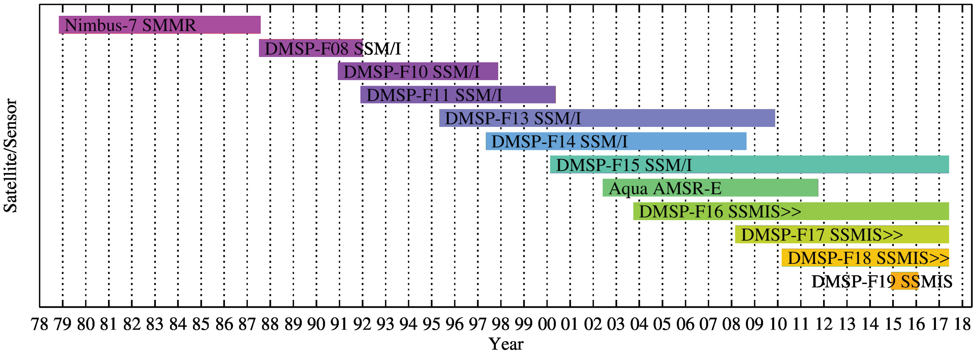
This paper describes standards and best practices that we used to produce the CETB data as a high-quality gridded brightness temperature ESDR [16]. The processed data include all SSM/I and SSMIS sensor record overlaps, some of which had never before been processed in gridded form (Figure 1). Spatial resolution of the CETB product has been enhanced up to 3.125 km for the highest-frequency radiometer channels, using the radiometer version of the Scatterometer Image Reconstruction (rSIR [17]) algorithm.

Section 2 describes the initial state of the software system we would modify to produce the new ESDR and identifies the changes that would be required. Section 3 identifies software production and data management best practices that we employed to produce the ESDR. Section 4 describes insights and lessons that may be derived from this ESDR production activity. Section 5 summarizes how the described work benefits users of the ESDR.

2. Background and Objectives

At the outset of the CETB ESDR development, the image reconstruction system [17,18,19] had been developed and tested in the C language at Brigham Young University, hereafter referred to as the “original system”. The ESDR development was planned to be performed on a new architecture at the University of Colorado, which would be capable of scaling to handle greater data throughput. The modified system, hereafter referred to as the “ESDR system”, would require significant changes to input and output subsytems, while maintaining the algorithmic integrity of the core image reconstruction algorithm. Figure 2 and Figure 3 describe the general designs of the original and modified systems.

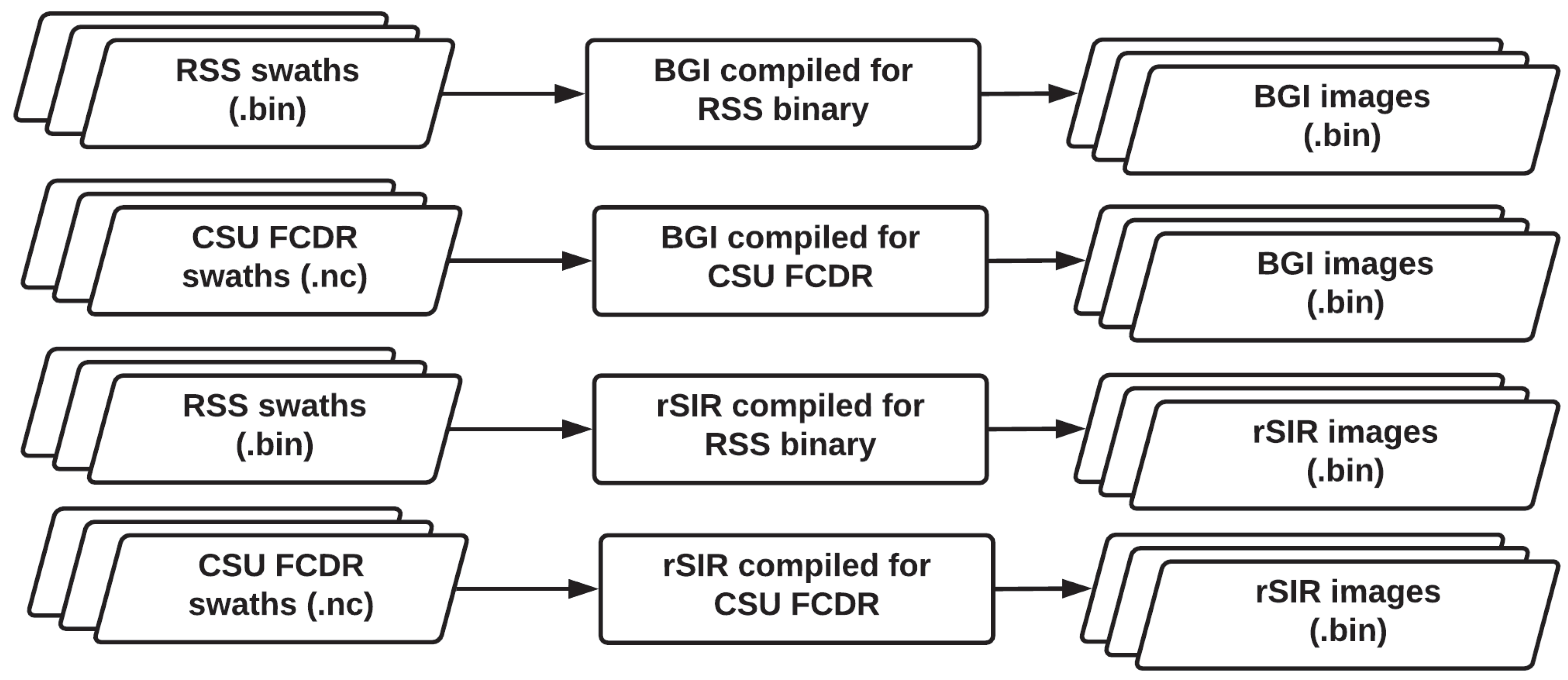
2.1. Original System Description

The original system had been implemented for two input sensor formats, SSM/I packed binary swath data produced by Remote Sensing Systems [20] and the CSU FCDR [14]. The switch between the two inputs was accomplished with conditional compilation, with conditional statements to handle differences in the data sources interleaved with image reconstruction implementation.

The original system included two potential image reconstruction algorithms, the Backus–Gilbert (BGI) method [9,10], and the radiometer version of Scatterometer Image Reconstruction (rSIR) method [18,19]. Our research required analysis and comparisons of outputs from both methods; details of the algorithm comparison [17] are beyond the scope of this paper.

Output of the original system comprised a set of data arrays, which included several large numeric arrays that had only been used during development exercises and would not be distributed to end users. The files were flat binary format, which required extensive ancillary understanding of the projection and grid. No processing or provenance metadata were saved with the data.

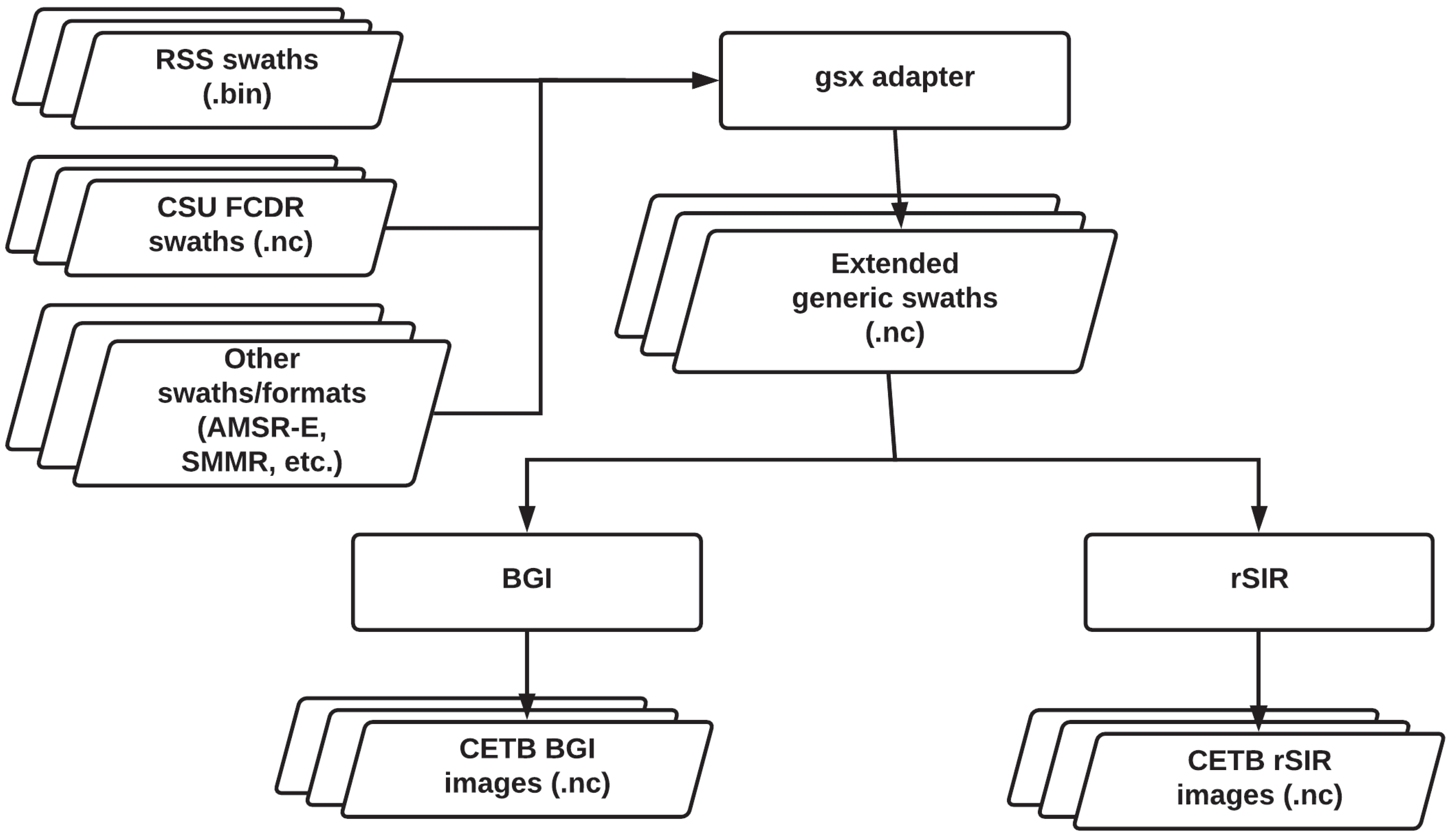
2.2. ESDR System Description

To produce the ESDR system, we needed to modify the original system to accept multiple new input sources. New input sensors were similar (but not identical) conical scanning radiometers, with different observational channels, various levels of auxiliary geolocation metadata, and input formats from various data producers, including netCDF, HDF, HDF-EOS, and packed binary format (

Table 1. CETB system input data sources. The original system only handled inputs marked with asterisks. The ESDR system was also required to input SMMR, AMSR-E, and SSMIS sensor data.

Name	Producer	Format	Reference
AMSR-E L2A	RSS	HDF-EOS	Ashcroft and Wentz (2013) [21]
SMMR Pathfinder	JPL	HDF	Njoku (2003) [22]
*SSM/I FCDR	CSU	NetCDF	Kummerow et al. (2013) [14]
SSMIS FCDR	CSU	NetCDF	Kummerow et al. (2013) [14]
*SSM/I V7	RSS	Packed binary	Wentz (2012) [20]
SSM/I FCDR	RSS	NetCDF	Wentz et al. (2013) [15]
SSMIS FCDR	RSS	NetCDF	Wentz et al. (2013) [15]

). The original system handled differences for input sensors in a fragmented fashion, with conditional logic in the reconstruction sections that violated the software design concept of separation of concerns. Our objectives for the new imput subsystem were: (1) to separate the input subsystem from the image reconstruction modules and handle any sensor and formatting differences as early as possible; (2) to simplify the image reconstruction algorithms by handling any sensor-specific logic during input; and (3) to remove the unwieldy conditional compilation mechanism to allow easier management of additional input sources.

Throughout the ESDR system modifications, we would need to preserve algorithmic integrity of the BGI and rSIR algorithms. Our objectives for the new algorithm subsystems were: (1) to ensure that any changes we made did not unintentionally alter algorithm results; and (2) to ensure transparency and reproducibility by capturing runtime processing parameters for inclusion in output file metadata.

We planned to produce ESDR output files using a self-describing format that would both capture relevant processing metadata, and would include descriptive metadata to improve usability and interoperability of the gridded data product. Image reconstruction can be employed to reduce noise or improve resolution, but both objectives cannot be achieved at once. We therefore produced relatively coarse-resolution, smoothed data at what has been considered the nominal “traditional” 25 km spatial resolution, and enhanced-resolution images at higher spatial resolutions, which varied by sensor and frequency (

Table 2. CETB ESDR gridded spatial resolutions, by sensor and measurement frequency. All data are produced as twice-daily EASE-Grid 2.0 images, as smoothed (25 km) grids, and at enhanced spatial resolutions as indicated here. Further details are available in the User Guide, available at http://nsidc.org/data/nsidc-0630.

Sensor	Frequencies (GHz)	Resolution (km)
		25	12.5	6.25	3.125
SMMR	6, 10	X	X
SMMR	18, 21	X		X
SMMR	37	X			X
SSM/I	19, 22	X		X
SSM/I	37, 85	X			X
SSMIS	19, 22	X		X
SSMIS	37, 91	X			X
AMSR-E	6, 10.7	X	X
AMSR-E	18, 23	X		X
AMSR-E	36, 89	X			X

). Our objectives for the ESDR output subsystem were: (1) to use a self-describing format to save relevant runtime and provenance metadata with the data files; (2) to employ the recently improved EASE-Grid 2.0 projections that simplified usability with common geolocation software; and (3) to include machine-readable projection and gridding metadata that typical geolocation software packages could interpret correctly.

Finally, the resulting ESDR data product was required to be delivered to the National Snow and Ice Data Center (NSIDC) Distributed Active Archive Center (DAAC). The DAAC data transfer required file-level metadata to be delivered with each data file. For the complete data set of over 3.7 million files representing daily grids for over 100 data years (totalling  53 TB), we needed a simple but robust migration process.

3. Methods

Knowing that the CETB data may be used for derived products and climate studies for many years to come, we defined the ESDR system and CETB data with specific attention to the following objectives:

• Preserving algorithmic integrity
• Input extendability
• Interoperability
• Usability
• Transparency
• Robust archive data migration

3.1. Preserving Algorithmic Integrity

In many ways, the work to produce an ESDR entails thoughtful separation of software-restructuring tasks that strictly preserve the algorithmic output of legacy software, from the new software features that will be required to produce high-quality ESDR products. Mens and Tourmé [23] point out the significant but necessary effort required to perform this activity, to gain a thorough understanding of the software system. Our initial engineering activity identified those parts of the system that would require modifications in order to meet our ESDR requirements.

The original system employed a packed binary output format that would require modification for multiple potential sensor data contents, and to include richer metadata that the NASA MEaSUREs program required. For the CETB product, we identified netCDF4 as a suitable format, due to its rich and extensible attribute capability and for the internal compression that the underlying HDF5 implementation would provide. We limited major software-restructuring tasks to the extraction and modification of input and output logic, while retaining the core algorithmic integrity of the image-reconstruction algorithms.

Our initial system development activities included the following steps that would undergird all of our subsequent workflow activities: (1) defining a suitable set of regression tests to ensure algorithmic correctness and preservation; (2) enabling continuous integration; and (3) practicing test-driven feature development with automated unit testing that was incrementally incorporated into continuous integration procedures.

3.1.1. Regression Testing

For regression testing, we depended on earlier algorithm development to have validated system correctness, and began with the assumption that reproduction of a representative sample of reconstructed images produced at Brigham Young University would be sufficient to demonstrate system preservation [23]. Our system would eventually be run on more than 100 data years of daily, global, swath data. The image-reconstruction processing was complex, and some parts of the original system performance were numerically slow. We decided to begin by making it run correctly, and then making it run fast if necessary to meet delivery schedules.

In order to facilitate reasonable performance during development activity, we defined two sets of regression testing output that we intended to execute at different times during integration: a quick regression that performed image reconstruction on a Northern Hemisphere subset of data from one channel and one day, and a more complete daily regression that processed all three targeted EASE-Grid 2.0 map projections (Northern and Southern hemisphere Azimuthal Equal-Area and Cylindrical Equal-Area to ±67 degrees latitude), for all observed channels and multiple spatial resolutions (Table 2). Regression tests passed if the brightness temperature data arrays were identical to within expected machine precision and compiler differences (<0.01 K on development virtual machines, or <0.05 K on the supercomputer, which used a different compiler). Precision differences of these magnitudes were only tolerated for fewer than 100 pixels per image.

To enable feedback during integration, we designed the quick regression to be as fast as possible. Our original performance target in the development environment was on the order of seconds to execute, but we settled for a test that seemed reasonably comprehensive for the full system logic, that ran in about 45 s. The more comprehensive daily regression required about 4 min. These long testing times are not optimal for fast development feedback, but we settled for the more comprehensive daily regression time, since it would be run asynchronously and automatically.

3.1.2. Continuous Integration

Software revision control is an indispensible tool for tracking changes to any software system. It represents the fundamental component of Continuous Integration (CI) systems [24], which we adopted to mitigate risk, automate repetitive processes, and ensure that changes to the system were not producing unintended changes to output. As basic workflow components of CI systems, individual developers concurrently work on separate system copies (branches) for bug fixes and feature development, documenting changes, performing builds and testing before commiting to a master branch for integration. Upon commitment of software changes, an automated build and testing are triggered on a machine dedicated to this task, thereby isolating the system build environment from behaviors that may be tied to a single developer’s environment. All tests must run successfully for the software to be considered in working order. Every change to the system that results in working tests triggers a new software tag that is written back to the source code.

At the onset of CETB development, we implemented the CI parts of the infrastructure prior to any software system changes, to ensure immediate detection of unintended processing changes. We include specific infrastructure software components that we used in

Table 3. Referenced software packages used during ESDR system development.

Name	Description	Website
ArcMap	Main component of ESRI ArcGIS	https://www.esri.org
Ceedling	C language unit testing framework	https://throwtheswitch.org
EPSG Registry	Map projection data base	http://www.epsg-registry.org
GDAL	Geospatial data abstraction library	https://www.gdal.org
Git	Distributed version control system	https://git-scm.com
Jenkins	Automated CI server	https://jenkins.io
Mapx	Map transformations library	ftp://sidads.colorado.edu/pub/tools/mapx
MCC	CF metadata compliance checker	http://podaac.uat.jpl.nasa.gov/mcc

. Quick regression tests are triggered automatically upon software commit actions, and the more demanding daily regression tests are scheduled to run daily at midnight.

Over the course of the project, our team of active, concurrent developers ranged from two to five core developers. If integration tests failed, developers on the project were notified by email. The development team was committed to correcting the problem in a reasonable period of time, which was usually accomplished before the next daily regression. If the problem were determined to be more serious than could be fixed quickly, the software was reverted to a prior working version. Successful daily regression tests therefore produced automated software releases, with the actual software version number automatically captured in output file metadata. No additional effort was required to make a new software release.

3.1.3. Test-Driven Feature Development

For new feature development in the CETB processing system, we used ceedling http://throwtheswitch.org, a C-language test-driven development framework. In test-driven development methods, small tests of desired behavior were written prior to source code changes, then incremental modifications to source code were made to make the tests pass. The process was repeated incrementally until the complete feature set was implemented [25]. This approach yielded several advantages to the product development. Without extra effort on the part of the developer, new development unit tests were automatically included in the integration testing process. Over time, this automated testing becomes insurance, in addition to the system-level regression tests, that subsequent modifications are not introducing undesired behavior.

3.2. Input Extendability

The original system was capable of handling two potential input sources, which had been implemented by use of conditional compilation. The CETB product was required to handle more sensors (Table 1), and to handle data that had been produced in multiple formats by different data producers. Furthermore, as we planned for future modifications, we wanted the system to be extensible to handle not only Fundamental CDR products, but also potential near real-time data sources. To manage these many multiple input forms, we adapted and upgraded the NSIDC generic swath (gs) system [26], which had been developed in the late 1990s.

The NSIDC gs system was originally implemented in C and used a flat binary storage format. Essentially an implementation of an Adapter software design pattern [27], the concept was an interface wrapper for swath format radiometer records; downstream gridding and subsetting software need only process a generic swath, or “gs”, version of the input data stream. While the pattern was useful for our purposes, the original gs structure definition lacked several elements required by the CETB image reconstruction algorithms. More significantly, modifications to the original gs structures would break backwards compatibility on several operational systems still in use at NSIDC. For CETB, we needed to adapt and extend the gs concept.

As the name implies, the eXtended generic swath (gsx) subsystem is based on the original gs Adapter design pattern, and makes use of netCDF4 for flexible and well-documented intermediate gsx swath file storage. Gsx is written in python, and was designed to be easy to extend with new translator logic when new inputs to the CETB system were identified. Newly developed for the CETB product, gsx was also developed within a test-driven framework, with a similar approach to continuous integration and automated testing.

Gsx provides a convenient encapsulation to handle sensor- or producer-specific idiosyncrosies, which simplified the original CETB core algorithms by removing special logic for handling input source file format and content differences.

3.3. Interoperability

We define the term interoperability as the ability of multiple systems and users to understand and make use of metadata and content information stored directly with the data. For each type of information that we wished to include, we considered which of various levels of metadata (file-level, variable-level) or supporting human-readable documentation would be most appropriate. In particular, complete map projection and gridding information was encoded in every file to ensure interoperability with geolocation-enabled software.

3.3.1. Use Machine-Readable Metadata

Machine-readable file formats enable interoperability with common software tools and multiple languages. Users can read files immediately using the language and tools with which they are most comfortable, rather than spending a long time, sometimes days or weeks, understanding a binary file format and writing customized, potentially error-prone, software to read and interpret unfamiliar projected data images.

For the CETB data files, we considered the HDF5 and netCDF4 formats. We selected netCDF4 because we were more comfortable with the conventions and terminology used in the netCDF4 application programming interface (API). Since netCDF4 is implemented with HDF5, we were also able to take advantage of powerful internal file compression capabilities of HDF5.

3.3.2. Climate and Forecast (CF) Conventions

We employed the Climate and Forecast (CF) metadata convention [28] to incorporate file-level, machine- and human-readable contents, geolocation, processing and provenance metadata. The CF convention was flexible and adaptable for including customized fields to describe our processing parameters and algorithm settings. We included runtime parameter settings that significantly affect reconstruction results, including number of rSIR iterations, gain thresholds for component measurements and local time-of-day thresholds that controlled temporal subsetting.

As an ESDR, the CETB product leverages as input a new, (swath format) FCDR, which includes a completely reprocessed historical SSM/I and SSMIS record including new efforts to improve intersensor calibrations [29,30,31]. To ensure transparency and reproducibility, we populated provenance metadata in file-level attributes in each CETB file at runtime, to record the specific FCDR files used to derive the CETB image; software version tags for the gsx and core systems were automatically captured as file-level attributes.

We made use of Dataset Interoperability Recommendations for Earth Science [32], which were approved and recommended for use by NASA in 2016, as general interoperability best practices for data providers. We incorporated several of these recommendations in CETB files, including (1) choosing a minimum set of CF variable attributes that included variable bounds, fill values, packing convention details, and units; (2) specifying spatio-temporal bounds attributes; and (3) including a degenerate time dimension, to enable NCO concatenation operators to easily aggregate gridded data arrays into space-time “cubes”.

While the CF conventions are powerful and flexible, the sheer number of attributes allowed by the convention can be extremely confusing to a data producer. We used a web-based Metadata Compliance Checker (MCC) to identify and correct CF compliance issues.

3.3.3. Include Geolocation Descriptions in Multiple Common Description Formats

Feedback to NSIDC repeatedly underscores the difficulties that users encounter in identifying projected data coordinates. For the CETB file definitions, we generally adhered to the DRY (Don’t Repeat Yourself) principle of software engineering, except for this important content. We deliberately violated the DRY tenet and included projection description information in the CF coordinate reference system (crs) variable attributes, as: (1) CF projection attributes; (2) PROJ.4 string; (3) EPSG ProjectedCRS code and EPSG Well-Known-Text (WKT) encoding; (4) the “grid parameter definition” (.gpd) filename used by NSIDC mapx software; and (5) references to peer-reviewed papers describing EASE-Grid 2.0. For example, in a 25 km Northern Hemisphere CETB file, the crs variable contains the following, highly redundant, information:

char crs ;

  crs:grid_mapping_name = "lambert_azimuthal_equal_area" ;

  crs:longitude_of_projection_origin = 0. ;

  crs:latitude_of_projection_origin = 90. ;

  crs:false_easting = 0. ;

  crs:false_northing = 0. ;

  crs:semi_major_axis = 6378137. ;

  crs:inverse_flattening = 298.257223563 ;

  crs:proj4text = "+proj=laea +lat_0=90 +lon_0=0 +x_0=0 +y_0=0 +ellps=WGS84

    +datum=WGS84 +units=m" ;

  crs:srid = "urn:ogc:def:crs:EPSG::6931" ;

  crs:references = [links omitted]

  crs:crs_wkt =

    "PROJCRS[\"WGS 84 /

    NSIDC EASE-Grid 2.0 North\",…"

  crs:long_name = "EASE2_N25km" ;

While we take a risk in violating DRY that we may erroneously include inconsistent projection parameters in various interpretations, we believe this risk to be outweighed by improved interoperability and comprehensibility, for a potential user who may only understand one method of defining the projection.

3.4. Usability

We define the term usability as the degree of ease with which a user can understand, analyze and manipulate the data product. During development, we used our Algorithm Theoretical Basis Document (ATBD) as a mutable record of the decisions we were making. Early versions of this document included a number of placeholder sections reserved for decisions that were not yet decided. As development progressed, we revised the ATBD to include our rationale for technical decisions, thereby documenting in the final released version of the ATBD [33] why we made the technical choices that we did.

We employed a volunteer community of gridded passive-microwave data users throughout the project for essential usability feedback. Our Early Adopters provided critical reviews of the contents of the ATBD and prototype versions of the data, which has been noted by the National Research Council as a critical element for CDR sustainability [3].

3.4.1. Use EASE-Grid 2.0

In recent years, the GeoTIFF metadata standard [34] has emerged as a popular format for embedding geolocation information into image files. However, none of the historical gridded passive-microwave data products could be formatted as GeoTIFFs without reprojection, because the cartographic projection ellipsoids did not match the WGS84 reference datum used for the source data geolocation [35]. This detail was not well documented in previously available passive-microwave gridded data sets. Many users were confounded by difficulties in understanding how to geolocate the data correctly. Specifically, Billingsley et al. [36] described complicated GDAL reprojection steps to correctly convert non-EASE-Grid 2.0 data with mismatched projection ellipsoids and reference datums to GeoTIFF. Similarly, Haran [35] described complicated steps required to properly import data with mismatched ellipsoid and datum into the Esri ArcMap geospatial analysis tool. The user in both of these cases needed expert knowledge in order to perform the reprojection without a datum shift. To be the most useful to the widest user community, we needed to make the CETB projected data understandable to software packages that assume the reference datum and projection ellipsoids are the same.

To improve usability of the gridded images in the CETB product, we employed the EASE-Grid 2.0 projection definitions. In the EASE-Grid 2.0 definition papers [12,37], we included appendices with implementations of the forward and reverse map projection transformations and the corresponding reference Open Source Geospatial Foundation (OSGeo) PROJ.4 string definitions. The three EASE-Grid 2.0 equal-area projections used for CETB (EPSG:6931-3) are defined with the European Petroleum Survey Group (EPSG) Registry. Users of any software that understands PROJ.4 strings and/or EPSG ProjectedCRS codes can now correctly geolocate the CETB product images, without fussy and potentially error-prone transformations or reprojections needed for use with other geolocated products.

3.4.2. Employ GDAL as a Usability Test

While adherence to conventions at a theoretical level is a necessary first step in improving usability of geolocated data files, the de facto demonstration of actual usability requires testing with current versions of targeted software. We decided to include sufficient standard geolocation information for the Geospatial Data Abstraction Library (GDAL https://www.gdal.org/) to produce compliant GeoTIFF images that software packages like GDAL and Esri https://www.esri.com/ ArcMap could easily import, understand, and analyze.

In the following example, the GDAL gdalinfo command-line utility correctly interprets the CETB CF-compliant metadata coordinate system:

$ gdalinfo NETCDF:"cetb_file.nc":TB_num_samples

Driver: Network Common Data Format

Files: cetb_file.nc

Size is 720, 720

Coordinate System is:

PROJCS["LAEA (WGS84) ",

  GEOGCS["WGS 84",

    DATUM["WGS_1984",

      SPHEROID["WGS 84",

        6378137,298.257223563,…

  AUTHORITY["EPSG","6931"]]…

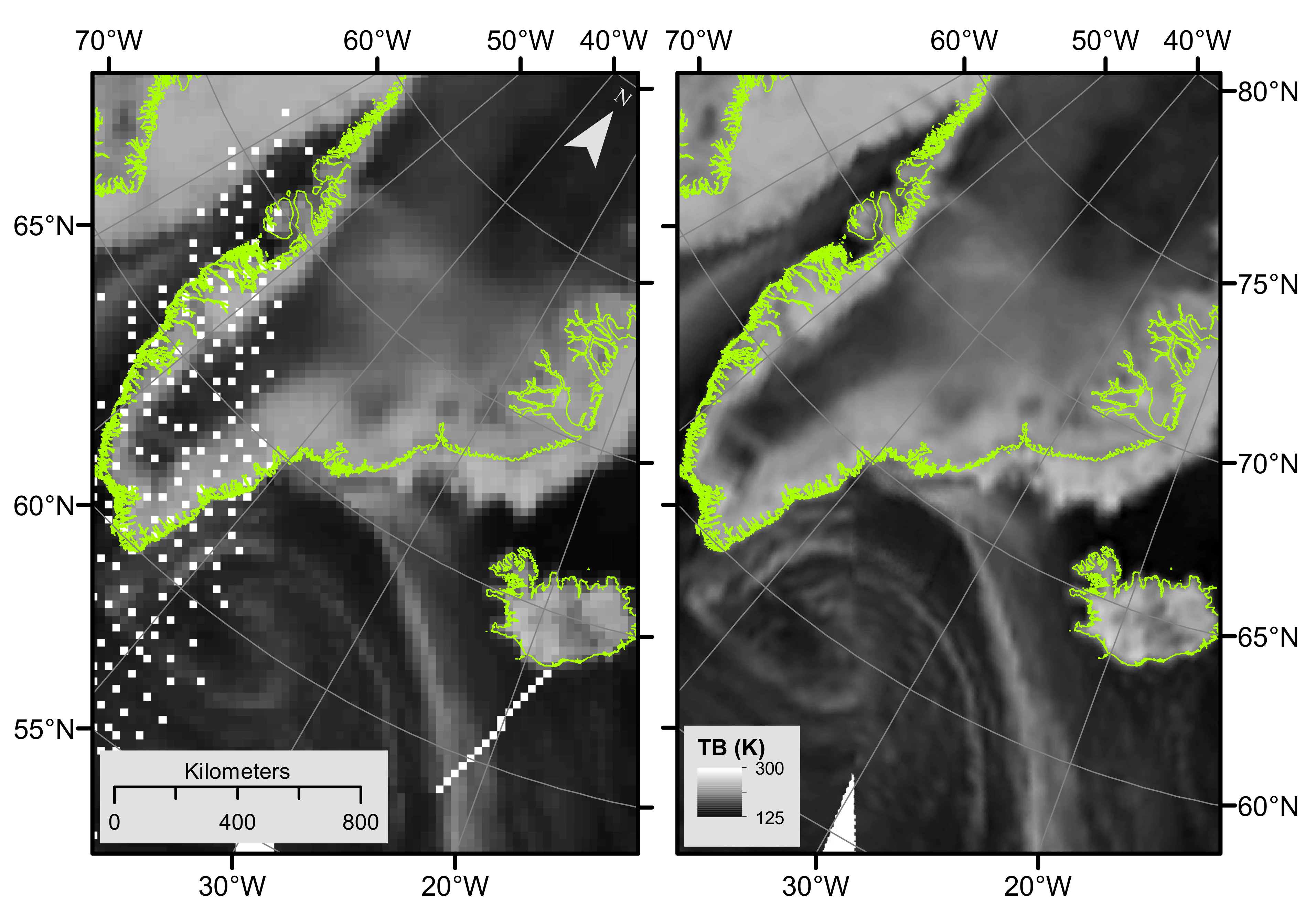
The command-line GDAL utility gdal_translate can then be used to extract the variable TB_num_samples from the CETB .nc file into a legal GeoTIFF. Since we have used the EASE-Grid 2.0 projections, no transformations for reprojection or datum shifts are necessary to overcome the problems that users of the historical gridded data have encountered in the past. By contrast, since we used netCDF and CF conventions to encode the EASE-Grid 2.0 projection definition and variable attributes, CETB users can simply instruct gdal_translate to interpret the file using NETCDF formatting:

$ gdal_translate \

  -of GTiff -b 1 NETCDF:"cetb_file.nc":TB_num_samples TB_num_samples.tif

Input file size is 720, 720 \

  0…10…20…30…40…50…60…70…80…90…100 - done.

The resulting GeoTIFF can be read and correctly reprojected without any further special instructions by any geospatial software that understands GeoTIFF, including but not limited to GDAL utilities and ArcMap (Figure 4).

3.5. Transparency

We define the term transparency in a data product as the degree to which necessary details in the product derivation have been included for a user to fully understand how data processing was performed. Satellite data records, like the passive microwave record, are subjected to several major reprocessing steps in conversions from detected voltages to usable geophysical parameters. As demonstrated by Eisenman et al. [38], undocumented changes in earlier data production methods, compounded with sensor transitions over time, raise challenges in teasing out real trends from spurious artefacts of processing methods. With the large number of potential derived climate records that depend on gridded brightness temperatures, we have placed a high priority on transparency to document details of our methods in producing the CETB. Any processing parameters that could change from file to file were included automatically at runtime in appropriate file- or variable-level attribute metadata.

Additionally, we included auxiliary data with the brightness temperature images, with pixel-wise processing statistics for number of measurement samples, average time and standard deviation of the measurements used to perform the image reconstruction, and the average incidence angle of the component measurements. Separately or in combination, these auxiliary statistics can be used to infer uncertainty of the reconstructed brightness temperatures. These statistics are provided to gridded data users for the first time with the CETB data; the historically available gridded products never included such information and therefore provided very few means of deriving temperature uncertainty.

3.6. Robust Archive Data Migration

Finally, the NASA MEaSUREs program designated the NSIDC DAAC (http://nsidc.org/daac) as the data repository for the CETB. Program-level support for data management at a trusted location like the NSIDC DAAC is critical to address the National Research Council recommendations for CDR sustainability [3] and for the data-management principles outlined by Parsons et al. [40]: to ensure that data be usable for complex, interdisciplinary science, it should be “discoverable, open, linked, useful and safe.” Early in the project, we established communications with the DAAC liaison to discuss expected data volumes, impact and general metadata and content. We used DAAC requirements for data archiving to generate file-level metadata required during the migration process. Data were delivered in subsets by sensor, using robust data transfer methods and a data manifest that included file-level checksums. The DAAC maintains user documentation (at http://nsidc.org/data/nsidc-0630) including citations to related publications and the ATBD [33] for production details, and manages a list of registered users who are notified of relevant data issues and developments.

4. Discussion

Data producers in many fields are developing best practices for data production and curation. For example, our practices overlap many elements in Goodman et al. [41], written for a computational biology audience. In our discussion of best practices that we leveraged to produce the CETB ESDR, we deliberately minimized details about specific technologies and emphasized the more general best practice that the technology du jour enables. For example, the basis of a good continuous integration system is a reliable revision control system that allows for concurrent development and automatic merging. The original references to the CI concept referred to Subversion https://subversion.apache.org, which in many communities has been superceded by git https://git-scm.com/ [42]. It is likely git will be replaced by something else in five or 10 years, but the best practice remains: that the use of a source-code revision-control system is a critical tool for reliable and automated data set development.

Likewise, there is great variety in automated servers for CI. For this project, we used Jenkins and a suite of virtual machines for development, CI and production. We found some aspects of this configuration to be fragile. For example, our first virtual machine implementations required nearly an hour to ensure we could rebuild machines with the required python packages installed, and the configuration of the CI machine that hosted the Jenkins server required extra manual steps. The delays that resulted from small changes to the virtual machines dragged on project momentum and interrupted the thought processes needed for actual changes to the CETB data. The complicated rebuild process made us less likely to rebuild for small system maintenance changes, which made the complexity and number of changes large by the time we were forced to rebuild machines.

We are migrating other projects away from this model, in favor of cloud-based CI pipelines, which are somewhat simpler and may require less maintenance over time. Ongoing work indicates that cloud-based alternatives may be more suitable for scaling to more complicated integration and regression testing scenarios, like the ones we required for CETB system development. There is, however, a cost in learning the cloud-based alternatives. As with revision-control systems, the specific technology is less important than the best practice: using an automated test and integration pipeline to free developers from repetitive but necessary tasks and to automatically identify integration problems as soon as possible after they are introduced.

As we transitioned the original software to an operational system to produce a reliable ESDR, we took pains to ensure algorithmic integrity by defining our automated regression testing. Despite the general recommendation to define tests that are fast, we settled for quick regressions that were not quick in practice. In hindsight, we found that this tended to slow down our testing feedback loops and interrupt workflow. In future we would recommend taking time at the beginning of the project to define truly quick, but not trivial, regressions. For our data production, this would have required manual editing of input gsx (swath) data files, to limit the computationally intensive calculations to only those measurements that intersected a small geographic area, for each of the three output projections.

We chose not to measure test coverage on our system. Given that our targeted changes would be to the input and output systems only, and that we were relying on regression testing for algorithmic consistency, we knew that coverage values would remain low for the overall system. A future improvement could include adding test coverage measurement to the daily automated processes, which would provide an incremental measure of improvement over time and changes to the system.

The gsx subsystem is fulfilling our intention to make the ESDR system easily extensible for new sensors and data sources, and to encapsulate details of any particular input format. We have recently completed a gsx extension to produce enhanced-resolution Soil Moisture Active Passive (SMAP) radiometer data, and have obtained funding to add near real-time data sources to the CETB system. Gsx can potentially be used to easily add data from similar radiometers to the ESDR system, including that of AMSR2 and WindSat.

5. Conclusions

We have described general best practices that we found valuable for CETB production. We adopted each practice to ensure that we were producing a high-quality ESDR that we expect the scientific community to use for many years. We used automated regression tests to ensure image-reconstruction algorithm integrity, even as we made necessary software changes to create an ESDR. A Continuous Integration system was invaluable to quickly detect unintended changes and to automate repetitive compilation and testing activities. We found test-driven development practices helpful for making required system modifications, and to increase testing coverage as we modified the system for new input sensors.

Our original core system employed a functional architecture. We nevertheless found it useful to borrow from object-oriented design pattern best practices. We used an Adapter design pattern to enable multiple input sensors and formats, and to encapsulate input-specific details early in the technical workflow.

CF Conventions were flexible and adaptable for including processing and provenance metadata in the final data product. To enable interoperability, usability and transparency, we published EASE-Grid 2.0 map projection details, complete with reference implementations and registration with EPSG, for popular software packages to correctly understand data geolocation. We deliberately violated the DRY principle in order to maximize geolocation usability for a diverse user community. We took care to document processing decisions and rationale at appropriate human- or machine-readable levels so that future users of the data will have enough information to understand what we did and why we did it. We used robust data-migration procedures to assure that what we produced is what the DAAC has archived. CETB ESDR data are freely available from the NSIDC DAAC.

Satellite passive-microwave brightness temperature observations are critical to describing and understanding Earth system hydrologic parameters that include sea ice extent and concentration, sea ice motion, snow water equivalent, snow and glacier melt onset and duration, soil moisture, surface water freeze/thaw states and precipitation. The low spatial resolution of historically available gridded products has precluded using these observations in regions with large brightness temperature gradients: at land-water and sea ice-ocean boundaries, along edges of ice caps and ice sheets, and in complex mountainous topography. Enhancing spatial resolution with image reconstruction, together with the systematic processing of the complete satellite observational record and the inclusion of pixel-level measurement and standard deviation statistics, should provide a rich data set with which to revisit analyses in these transitional regions. The complete v1.3 CETB ESDR has been available from the NSIDC DAAC since June 2018. Current studies are underway to evaluate the potential improvements the CETB ESDR may enable in derivations of sea ice concentrations and extent, in melt onset and duration in mountainous terrain and in highly complex Arctic archipelagos, and to improve snow water equivalent estimates in mountainous regions. We expect the CETB ESDR to better serve the needs of derived products, as a fully transparent, well-documented, reliable gridded product that has now been systematically processed at enhanced spatial resolutions.