Range Image Technique for Change Analysis of Rock Slopes Using Dense Point Cloud Data

Abstract

The use of a terrestrial laser scanner is examined to measure the changes of rock slopes subject to a wave attack test. Real scenarios are simulated in a water flume facility using a wave attack experiment representing a storm of 3000 waves. The stability of two rock slopes of different steepness was evaluated under the set conditions. For quantification of the changes of the slopes after the wave attack test, terrestrial laser scanning was used to acquire dense 3D point cloud data sampling for slope geometries before and after the wave attack experiment. After registration of the two scans, representing situations before and after the wave attack, the cloud-to-cloud distance was determined to identify areas in the slopes that were affected. Then, a range image technique was introduced to generate a raster image to facilitate a change analysis. Using these raster images, volume change was estimated as well. The results indicate that the area around the artificial coast line is most strongly affected by wave attacks. Another interesting phenomenon considers the change in transport direction of the rocks between the two slopes: from seaward transport for the steeper slope to landward transport for the milder slope. Using the range image technique, the work in this article shows that terrestrial laser scanning is an effective and feasible method for change analysis of long and narrow rock slopes.

1. Introduction

The protection of coastal zones is fundamental to the effective operation of local socioeconomic activities, especially in the Netherlands, a lowland country with significant coast length. For example, the risks of coastal erosion are expected to increase [1] due to predicted climate change the associated sea level rise, tidal effects, and expected increases in the intensity and frequency of storms. Conversely, coastal erosion poses a serious threat to the nature hazard agents. Various types of coastal elements, i.e., sand banks, sandy beaches, and dunes [2,3], have been used to protect coastal areas from erosion, most of which are made by rockfill [4,5,6,7,8]. With the rapid erosion of coastal structures, demand for natural rocks has increased around the world [9].

A problem that has drawn the attention of researchers involved in coastal protection is which configuration of rocks provides optimal protection in a given wave climate scenario all the time [10]. An extensive review of laboratory studies employing random waves was performed on the stability of so-called riprap slopes [11]. The stability of rock slopes consisting of loose rocks under wave attack has been investigated before [10]. The stability of rock slopes in the range from 1:1.5 to 1:4.0 were tested by performing 250 tests, the results presented the probability distribution of run-up on rock slopes [12]. The abilities and limitations using dynamic stability formulas for breakwater profile change under random waves was obtained using the experimental data [13]. These older tests typically used a mechanic profiler to obtain approximately 10 transects of the profile development and, thereby, did not capture the full redistribution of bed material. In later research, the rates and mechanisms of changes in rock slopes were also examined by distinct element computer modeling using field and laboratory data [14]. A detailed structural analysis was performed by a digital elevation model using COLTOP-3D software for rock slope relief [15].

More recently, the accuracy of techniques such as digital terrestrial photogrammetry and terrestrial laser scanning was assessed in rock slope stability analysis [16]. Measurements extracted from a 3D digital stereo photography were applied to evaluate damage parameters for rock slopes of a water flume [17]. The damage to 3D rubble mound structures was also described and quantified in Hofland et al. [18]. The same technique was extended by refraction step to enable bathymetric monitoring in a laboratory environment [19]. The settlement of single-layer rock armor layers of coastal structures was quantified, analyzed, and presented using imaging processing techniques [20]. The effect of an oblique wave attack on rubble mound breakwaters was tested using stability formulae. The results indicated that the influence of oblique waves was larger for long-crested waves [21]. The same technique was applied in the evaluation of the stability of cube armored roundheads exposed to long- and short-crested waves [22]. In this evaluation, a configuration of two layers of randomly placed cubes was considered with respect to variations in ranges of head diameter, slope, cube mass density, and wave steepness. Despite such progress in rock measurement, an improved assessment of rock slopes and other coastal structures is urgently needed for a more detailed insight in rock movements and changes.

Terrestrial laser scanning (TLS) offers high accuracy and high speed data acquisition resulting in dense point clouds, thereby allowing the detection of changes, even microchange, in repeatedly scanned data [23]. The technique of TLS has been widely used in structural change analysis [24], evaluating deformations [25] or assessing geometric changes [26,27,28,29,30,31,32], detection of the level of damage in masonry buildings [33], and natural hazards [34,35,36,37]. The accuracy of some types of TLSs have been assessed such as Faro Focus 3D and Leica HDS6100 [38], Faro 880 [39], Leica C10 [40,41], Trimble GX, and Riegl LMS420i [42]. In the past decade, the use of laser scanner seems to be established in coastal engineering, e.g., for measuring waves [43,44,45,46], for assessing sand transport on sandy beaches [47], and for measuring rocks [48,49,50]. The use of TLS has been consolidated in the analysis of rock slopes [50]. For example, Abellán et al. (2014) [48] have reviewed the applications of TLS in rock slope characterization and monitoring, in which the development of new algorithms for deformation tracking and change detection using point clouds was summarized. TLS was used to monitor susceptibility of coastal cliffs in terms of angles and ground fall, the results of which provided input to establish boundaries of safe investments zone or retreat infrastructure like buildings in case of real threat by creating a warning system from the collected point cloud data [51]. A new approach of coastal cliff monitoring was proposed previously [52], which combined mobile scanning from the sea with a geotechnical stability analysis to form a new comprehensive monitoring system. A quantitative analysis was carried out using TLS combined with airborne laser scanning to implement slope propagation models, with which the parameters influencing the behavior of a rock mass was measured [50]. TLS was used to extract geometry and monitor change in rubble mound breakwaters, which are coastal defense structures designed for protecting harbors and beaches from the impacts of storm waves [53]. TLS was also performed to evaluate short-term changes in Cubipod armored breakwater roundheads, and it has been found to be an accurate technique for damage monitoring in breakwaters [54]. Furthermore, a geometrical analysis was performed using laser scanning and photogrammetric point cloud to identify discontinuity sets of rock slopes [49] and the techniques have been found to deliver reliable results.

We discussed an earlier application of TLS for change analysis of rock slopes in [55]. That framework included registration of two point clouds, coordinate transformation from the TLS coordinate system to the so-called slope coordinate system, range image creation, and change detection. However, this framework has two main drawbacks. First, the applied registration and coordinate transformation will introduce small alignment errors, and even minor errors may lead to erroneous changes in the detection results, especially when the magnitude of the change value is relatively small. Second, different pixels in the raster image have identical size but the number of points per pixel has significant differences. In other words, the point density varies which results in local variations in change detection accuracy. To solve these drawbacks related to misalignment and non-uniform accuracy, we propose to introduce the range image technique for change analysis. In this article, the use of a laser scanner to obtain change information is examined and its applicability is confirmed. The aim of the present article is to understand how coastal structures with gentle slopes behave during a wave attack. First, the wave attack test and the scan data acquisition are discussed. Next, to guarantee the accuracy of the change analysis, point cloud registration before and after the wave attack test is performed using the control points method. To identify the area within the entire slope where significant change occurred, the cloud-to-cloud distances between the different slope point clouds are estimated using the CloudCompare software [56]. To obtain further insight in the changes in the affected area, a so-called range image is created based on the vertical and horizontal angular resolutions of the point clouds. Subsequently, quantification of changes is carried out on the two slopes to see how the rock slopes behave against the wave attack.

In this article, first the wave flume and the wave attack tests are described in Section 2.1, and how the dense point cloud is acquired using a Leica C10 scanner. Next, Section 2.2 explains the methodology performed in this article, which is composed of five main steps: (1) point cloud registration between two epochs; (2) damage area detection using cloud-to-cloud distances; (3) range image creation for the interest area; (4) quantification of changes; and (5) volume change estimation. In Section 3, the results are presented and analyzed. Afterwards, a discussion of the effectiveness of the method is provided. Finally, in Section 4 conclusions and future work are presented.

2. Materials and Methods

2.1. Materials

2.1.1. Wave Attack Simulation

In the experiment considered, wave attacks on two types of rock slopes (V:H) were performed, 1:10 and 1:5, respectively. These two types of slopes were assessed considering their safety against wave attack as a guide for the construction of coastal structures. The slopes were tested under set wave conditions to determine their stability in the water flume of Delft University of Technology, which has a length of 40 m, width of 0.8 m, and a height of 0.9 m. Their stability on its turn is derived from the profile change after a wave series that present a Dutch storm event including 3000 waves. The wave heights for slopes of 1:10 and 1:5 are 0.129 m and 0.054 m, respectively. Since the experiment was conducted in a laboratory, artificial lighting from the ceiling was presented. At each occasion, the slope was scanned before the wave attack, and afterwards, after the water was removed from the flume. To mount the terrestrial laser scanner directly above the rock slope, a special wooden construction was made, see Figure 1a. In the tests, the placed wooden construction was regarded stable during each scan.

To simulate real coastal conditions, the wave surface did not cover the entire slope as can be seen in Figure 2, where oblique surfaces surrounded by solid lines are rock “Slope 1” (1:10) and rock “Slope 2” (1:5), respectively. The blue dashed line represents the wave surface in the still state. The red dashed lines indicate the intersection line (coast line) between still wave level and the two rock slopes, respectively.

The water flume was designed for modeling coastal structures and assessing their safety against wave attack, storm surges, and flooding. As shown in Figure 2, a special wave maker was set at the right side of the water flume. The wave generator paddle at a 0° angle wave attack provided mechanically irregular waves on the flume. The generator was controlled by a computer program [57]. The program was developed for simulating regular, irregular, and a variety of other wave conditions. In our experiment, a Dutch storm of 3000 waves was generated by the JONWAP (Joint North Sea Wave Project) wave spectrum.

In this experiment, two mild slopes (1:10 and 1:5) were tested under set wave conditions to determine their stability. The stones used on the slopes have a nominal diameter of 16.20 mm and were placed at a layer thickness of two times the nominal diameter (i.e., 32.40 mm). The shape of the stone were determined by their length-to-thickness ratio, their blockiness, their roundness, or their cubocity, as described in the Rock Manual [58].

2.1.2. Point Cloud Acquisition

The experiment was performed from 14 August 2016 to 28 September 2016. Repeated scanning was done before and after the wave attack testing. A C10 Scan Station scanner (Leica, Heerbrugg, Switzerland) was used for this experiment. The Leica C10 Scan Station scanner, with an effective range of 280 m at 90% reflectively, exploits a time-of-flight principle for measuring the range between the scanner and the object. The accuracy of a single measurement is 6 mm (one sigma) in position and 4 mm (one sigma) in depth at ranges up to 50 m [59]. For each epoch, two scans were made. The first scan was made based on a minimum resolution corresponding to 0.2 m in horizontal and vertical spacing when the range is 100 m [40], and with a complete field of view, i.e., 360 arc-degree with respect to the Z-axis and 270 arc-degree for vertical amplitude. While the second scan was made based on a high-resolution with an area only including the water flume, in which the high-resolution corresponds to 0.05 m in horizontal and vertical spacing at a range of 100 m.

Table 1. Number of points of processed scans.

Slope Type	Number of Points
	Before	After
1:10	2,508,761	2,673,580
1:5	1,979,464	2,007,694

describes the point clouds acquired for two slopes.

The location of the scan position was set on the top side of the slope. To guarantee the accuracy of the registration, three targets with relatively strong geometry were positioned on the water flume frame, see the right figure of Figure 1. In this figure, the positions of the scanner, the targets and the slope are indicated in a scanner view of the experiment scene.

2.2. Methodology

The methodology is based on the dense point cloud of the rock slope before and after the wave attack test. A workflow summarizing the methodology is presented in Figure 3 and the steps are described in the following paragraphs.

2.2.1. Registration of Two Epochs

In general, the locations of the scanning stations were not strictly the same at the different epochs, so the coordinates acquired in two consecutive epochs are not expected to be at the same reference system with different origins and/or orientation. Thus, the registration of point clouds from two epochs is required before change analysis can be performed. Registration aligns and combines multiple point clouds into a single set of range data. However, the introduced registration error will inevitably affect the change detection results, even though the magnitude is relatively small.

In our research, the control points method (TCP) is employed for the process of registration of various scans. Three targets made by special materials manufactured by the Leica Company (Wetzlar, Germany) are used, the centroid of which can be extracted by the scanner itself in a highly accurate way. In this way, the Leica Cyclone software could provide an automatic registration based on TCP. Considering the characteristic of the water flume with long length compared to its width, it is difficult to position the targets in a geometrically strong way. However, due to the high accuracy of target center extraction algorithm by Leica Cyclone software, a high-precision registration could be performed using the Least Squares method: the errors for the three targets between two epochs are less than or equal to 1 mm.

2.2.2. Cloud-to-Cloud Distances

As a clean and proper model of a subject surface is difficult to obtain, the classical way to detect changes from point clouds is cloud-to-cloud distances based on local neighbors [60]. This is a fast and direct 3D comparison method that has been widely applied in point cloud comparison. The method has the advantage that it does not require meshing of the dataset, nor estimation of point normals. For each point in the evaluated point cloud, the nearest point in the reference cloud is searched and the Euclidean distance between them is computed. Direct point to point comparison has at least two disadvantages: results are often noisy, and results are dominated by local point spacing. Alternatively, from one point cloud a surface approximation is estimated. The process is first to find the nearest point in the reference cloud. Based on the nearest point and its predefined number of neighbors, the surface of the reference is modeled locally by fitting a mathematical primitive like a plane. The distance to this local model is finally determined. A graphical diagram illustrating the local of a local surface model for cloud-to-cloud distances is shown in Figure 4.

One advantage of using cloud-to-cloud distances for change detection is that it does not require the explicit pairing of point in two datasets [61]. However, cloud-to-cloud distances are always positive which means that the direction of change is still unknown.

2.2.3. Range Image and Raster Image Creation

Actually, the scanner mechanism can be considered to operate in a spherical coordinate system. In most current systems, the point cloud acquired is expressed in Cartesian coordinates, which means that the original acquisition organization is lost. Therefore, this unorganized cartesian representation is converted to spherical coordinates before further processing. As a result, the unorganized 3D data are expressed in a 2D range image format. The angular resolution $\Delta \theta$ is predefined depending on the scanning resolution that can be regarded as inherent parameter of the scan. For searching in a simplified way, a conversion is made to generate regular raster (2D coordinates) [62]:

$$\begin{array}{l}\theta =\frac{1}{\Delta {\theta }_H}\arctan \frac{Y}{X}\\ \phi =\frac{1}{\Delta {\theta }_V}\arctan \frac{Z}{\sqrt{X^2+Y^2}}\end{array}$$

(1)

where $\theta$ and $\phi$ are the 2D spherical coordinates of a point derived from the 3D coordinates; $X$, $Y$, and $Z$ are the 3D Cartesian coordinates as gathered by the scanner; $\Delta {\theta }_H$ and $\Delta {\theta }_V$ are the horizontal and vertical angular resolutions, respectively, which depend on the scanner settings. The range from the point to the scanner center is determined by $\rho =\sqrt{X^2+Y^2+Z^2}$. In such a coordinate system, the 2D coordinates of all points are organized in a 2D array indexed by row and column number.

In contrast, for a point $P_i\left({\theta }_i,{\phi }_i,{\rho }_i\right)$ in the range image, the corresponding Cartesian coordinates can be expressed as

$$\begin{array}{l}{X}_i={\rho }_i\cos \left({\phi }_i\Delta {\theta }_V\right)\sin \left({\theta }_i\Delta {\theta }_H\right)\hfill \\ Y_i={\rho }_i\cos \left({\phi }_i\Delta {\theta }_V\right)\cos \left({\theta }_i\Delta {\theta }_H\right)\hfill \\ Z_i={\rho }_i\sin \left({\phi }_i\Delta {\theta }_V\right)\hfill \end{array}$$

(2)

Since there is no absolute corresponding point between two epochs of the same scene, the raster image is generated to realize the change in value acquisition by comparing the corresponding grid at the same location in different epochs. Once the point cloud is in this 2D space, the next task consists of converting this dataset, composed of isolated points, into a raster image where the size of the grid in the raster image is predefined by the user, depending the angular resolution and practical necessity. In this raster image, the attribute of each grid is the mean range obtained by averaging all ranges of points in the current gridded. Assuming that the pixel size is $k$ times the angular resolution, the size of the bounding box is $k\Delta {\theta }_H\times k\Delta {\theta }_V$, which denotes the resolution of the raster grid cells. It should be noted that the resolution here is not the real dimensions in 3D space, but the dimensions related to angular resolution in range image as introduced above. In practice, the user can fix the resolution of the pixel size or estimate it depending on the point cloud density in the 2D space. Consequently, a raster grid of size $m\times n$ was built, where $m$ is the number of rows and $n$ is the number of columns.

2.2.4. Quantification of Changes

Once the raster images for both point clouds are created, the range change is subsequently tracked by comparing the corresponding cells in two different epochs, which is computed as

$$\Delta \rho ={\rho }_2-{\rho }_1$$

(3)

where ${\rho }_1$ and ${\rho }_2$ denote the ranges to the scanner center for the first and second epochs, $\Delta \rho$ is the range change between two epochs.

Although the range change for each cell was estimated, the change along or perpendicular to the slope is still unclear. For further exploiting the change information, it is better to project the range change to the directions along the slope and perpendicular to the slope, the details of this process are as follows.

(1)

Slope direction determination. As shown in Figure 1, the scanner is mounted at the middle along the cross section of the trunk. In such a case, the cells at the middle of the water flume along the slope direction have the same horizontal angle in the range image. Subsequently, the horizontal angle (${\theta }_M$) representing the slope direction is obtained by averaging the horizontal angles of all cells in the range image. By connecting the cells with the same horizontal angle ${\theta }_M$ the slope direction is determined. Afterwards, the 3D points in the current cells representing the slope direction are extracted. Using the points in 3D space, the vectors for the direction are estimated by means of Principle Component Analysis (PCA), the principle of which is shown in Jolliffe [63] in detail. Here, we define the direction away from the scanner as the position direction (down-slope). A vector $V_1$ is used to represent the slope direction.

(2)

Direction across the water flume determination. Once the slope direction is determined, the next step is to determine the section direction. It is apparent that the section direction is perpendicular to the slope direction, so the key is to determine the position direction of the section. In our research, the direction from the left to the right from the viewpoint of the scanner is regarded as the positive direction of the section. A vector $V_2$ is used to represent the section direction.

(3)

Direction vertically upwards against the slope plane. The direction ($V_3$) is pointing upwards perpendicular to the slope plane determined by the vectors $V_1$ and $V_2$, which is simply given as

$$V_3=V_1\times V_2$$

(4)

where ‘×’ denotes cross multiplication.

Once we have defined the changes in the three directions $V_1$, $V_2$, and $V_3$, we could project the range change to the three directions, as presented subsequently.

Indeed, the range for a cell in the range image is the distance from the location of the current cell to the scanner center. In this sense, the range also could be expressed by a vector connecting the current cell to the scanner center. Let $P_i\left(X_i,Y_i,Z_i\right)$ denote the 3D Cartesian coordinates for the current cell. As the 3D Cartesian coordinates of the scanner center are always $O\left(0,0,0\right)$, the range direction is therefore expressed as $P_{i}O\left(-X_i,-Y_i,-Z_i\right)$.

Subsequently, the range change projection is performed according to Equation (5).

$$\begin{array}{l}{L}_x=\Delta {\rho }_i\cdot P_{i}O\cdot V_2/\Vert V_2\Vert \\ L_y=\Delta {\rho }_i\cdot P_{i}O\cdot V_1/\Vert V_1\Vert \\ L_z=\Delta {\rho }_i\cdot P_{i}O\cdot V_3/\Vert V_3\Vert \end{array}$$

(5)

where $\Delta {\rho }_i$ is a scalar denoting the range change for the current cell, $P_{i}O$, $V_1$, $V_2$, and $V_3$ are vectors, and $\Vert •\Vert$ is the norm of a vector.

2.2.5. Volume Change Estimation

Once the range change is obtained, volume change detection is performed based on the cells in the raster image. Given a cell $C\left(i,j\right)|i=1,2,\cdots ,m;j=1,2,\cdots ,n$ in the raster image, the 2D coordinates of four corners are determined, i.e., $A_1\left({\theta }_1,{\phi }_1\right)$, $A_2\left({\theta }_2,{\phi }_2\right)$, $A_3\left({\theta }_3,{\phi }_3\right)$, and $A_4\left({\theta }_4,{\phi }_4\right)$. Next, the 3D coordinates of the four corners ($B_i\left(X_i,Y_i,Z_i\right)|i=1,2,3,4$) in Cartesian coordinates are computed according to Equation (1). The cell in 3D space is regarded as a rectangle, the area ($S_{ij}$)is therefore calculated using the 3D coordinates of four corners. Finally, combined with the change value vertically upwards against the slope plane provided by the previous step, the volume change is estimated as $\Delta V_{ij}=L_z\cdot S_{ij}$. Here we should remark that the cell projecting back to the 3D space is not rigorously a rectangle but an annulus sector (Figure 5), which can be approximated by a trapezoid since the angles $\Delta \theta$ are close to zero. Namely when $\Delta \theta \to 0$, the chord and arc with respect to the identical angle are with nearly equal values of length. As illustrated in Figure 5, the current red cell in raster image is described by four corners $A_1$, $A_2$, $A_3$, and $A_4$ while the corresponding area in the 3D space is represented by $B_1$, $B_2$, $B_3$, and $B_4$, such that

(1)

$B_1$ and $B_2$ have the same vertical angle;

(2)

$B_1$ and $B_3$ have the same horizontal angle;

(3)

$B_3$ and $B_4$ have the same vertical angle; and

(4)

$B_2$ and $B_4$ have the same horizontal angle.

In fact, the connection of points $B_1$ and $B_2$ is an arc rather than a chord (straight line). The same holds for the connection between points $B_3$ and $B_4$. In addition, the length from $B_1$ to $B_2$ is not strictly equal to the length from $B_3$ to $B_4$ as they have the same horizontal angular difference but a different vertical angular difference in 3D space. However, the cell size is relatively small, that is, the length difference induced by the vertical angular difference is small enough to be ignored. Given that in our experiment, the maximum range in the scene is less than 20 m, the cell in 3D space is treated as a rectangle in the later process without compromising the final accuracy.

3. Results

3.1. Registration

As mentioned in Section 2.1, three plane targets were set for aligning the point clouds from different epochs. Control points were additionally measured by the scanner, to align the scans more accurately to a common reference system for the coordinates. The errors for the registration in Slope 1 are 0.000, 0.001, and 0.001 mm along the X, Y, and Z axes, respectively. While in Slope 2, the errors are 0.001, 0.000, and 0.000 mm along the X, Y, and Z axes, respectively. These errors indicate that the registration was performed with high precision for two slopes, which therefore guarantees the reliability of change detection results in the same reference system.

3.2. Change Analysis Using Cloud-to-Cloud Distances

Once two 3D point clouds are spatially registered for two slopes, they can be compared against each other for change analysis. Thus, the cloud-to-cloud distances for the two slopes were calculated using the CloudCompare software [56] and the resulting scatter diagrams colored by distance value are shown in Figure 6 (for slope 1) and Figure 7 (for slope 2), respectively. As the stones on the slope do not have regular shapes, a least squares best fitting plane may not always be a good approximation. Therefore, quadric fitting of local surfaces is employed in our study. When searching for the k-nearest neighbors (k-NN) points, six nearby points were used. In the case of Slope 1 (1:10), the maximum cloud-to-cloud distance was 0.0333 m, while for Slope 2 (1:5) the value was 0.0206 m. The cloud to cloud distances variation distribution is summarized for Slope 1 and Slope 2 respectively, see

Table 2. Distribution of cloud to cloud distances for Slope 1.

Distance Interval (m)	0–0.003	0.003–0.006	0.006–0.009	0.009–0.012
Number of points	2,505,973	103,628	42,993	14,816
Distance interval (m)	0.012–0.015	0.015–0.018	0.018–0.021	0.021–0.024
Number of points	4649	1137	252	95
Distance interval (m)	0.024–0.027	0.027–0.030	0.030–0.033	all
Number of points	28	8	1	2,673,580

and

Table 3. Distribution of cloud to cloud distances for Slope 2.

Distance Interval (m)	0–0.003	0.003–0.006	0.006–0.009	0.009–0.012
Number of points	1,963,455	33,476	8732	1715
Distance interval (m)	0.012–0.015	0.015–0.018	0.018–0.0206	all
Number of points	166	95	55	2,007,694

.

For Slope 1, the number of points with a cloud-to-cloud distance less than 0.003 mm is 2,505,973, which accounts for 93.7% of all points of the slope (Table 2). While in the case of Slope 2, this percentage is 97.8% as can be inferred from Table 3. This indicates that a relatively small change occurred at most of the surface of each slope. As seen from Figure 6 and Figure 7, larger changes occurred near the intersection line for both slopes, which indicates the region most affected by the wave attack. A possible explanation for this phenomenon is that the location near the intersection line is influenced significantly by the series of waves, and the runup and rundown velocities in this location are highest compared to the other areas. By estimating the cloud-to-cloud distances, the affected area and the associated change values could be identified. Noteworthy, the cloud-to-cloud distances are absolute values, and therefore the direction of change cannot be detected. That is, in our case the erosion or dilation for the rock slopes cannot be distinguished.

3.3. Range Image Technique for Quantifying Change Regions

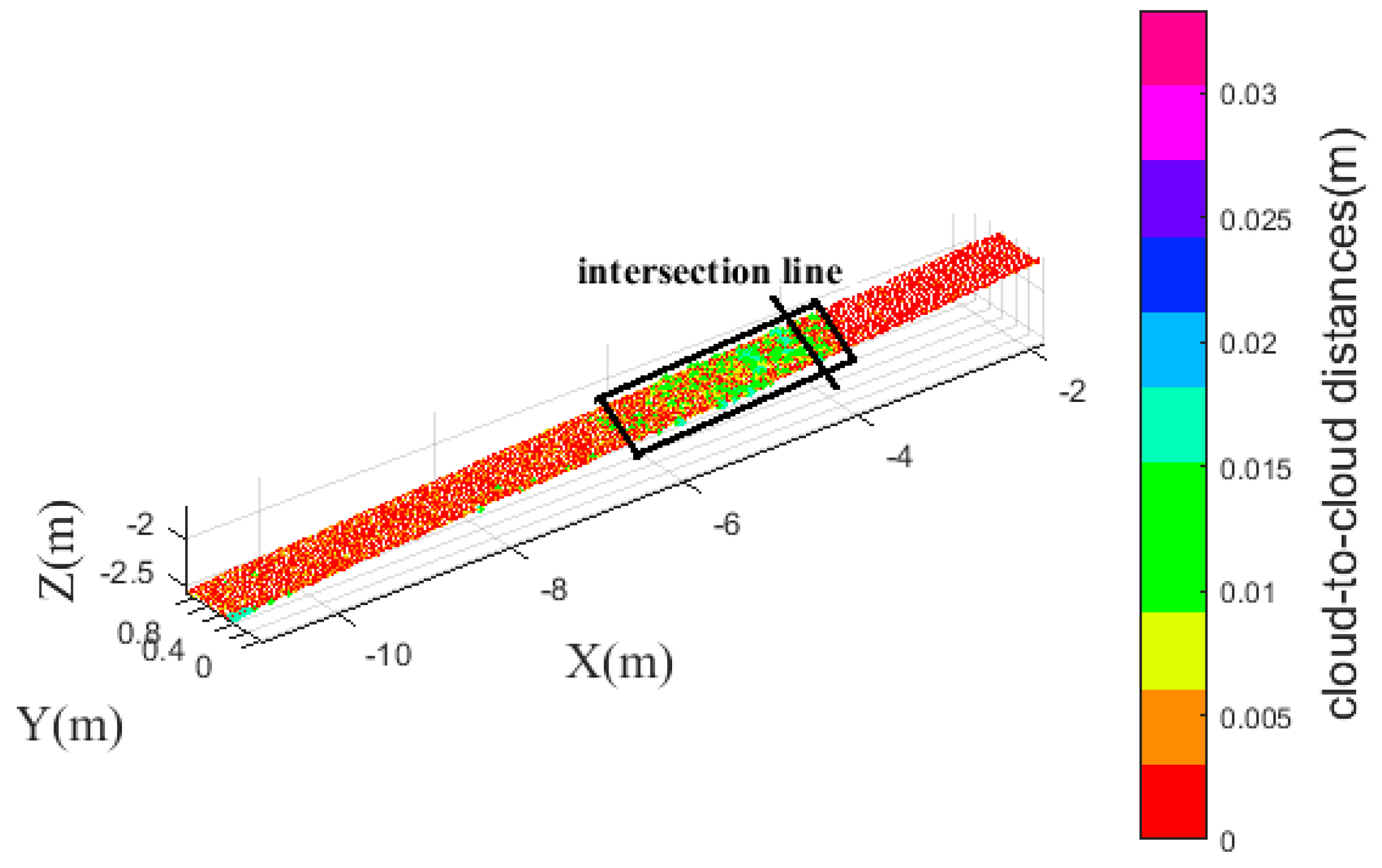
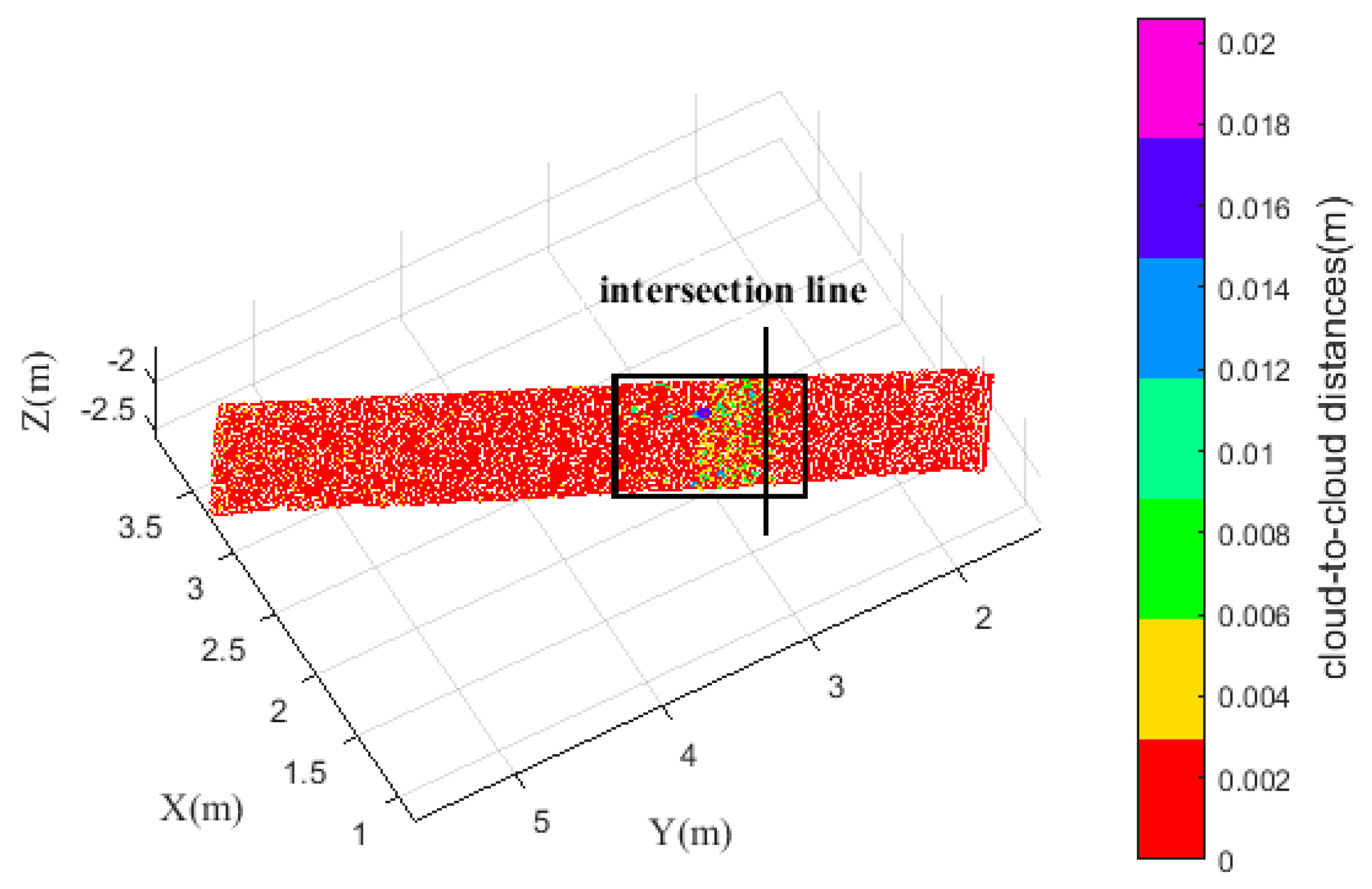
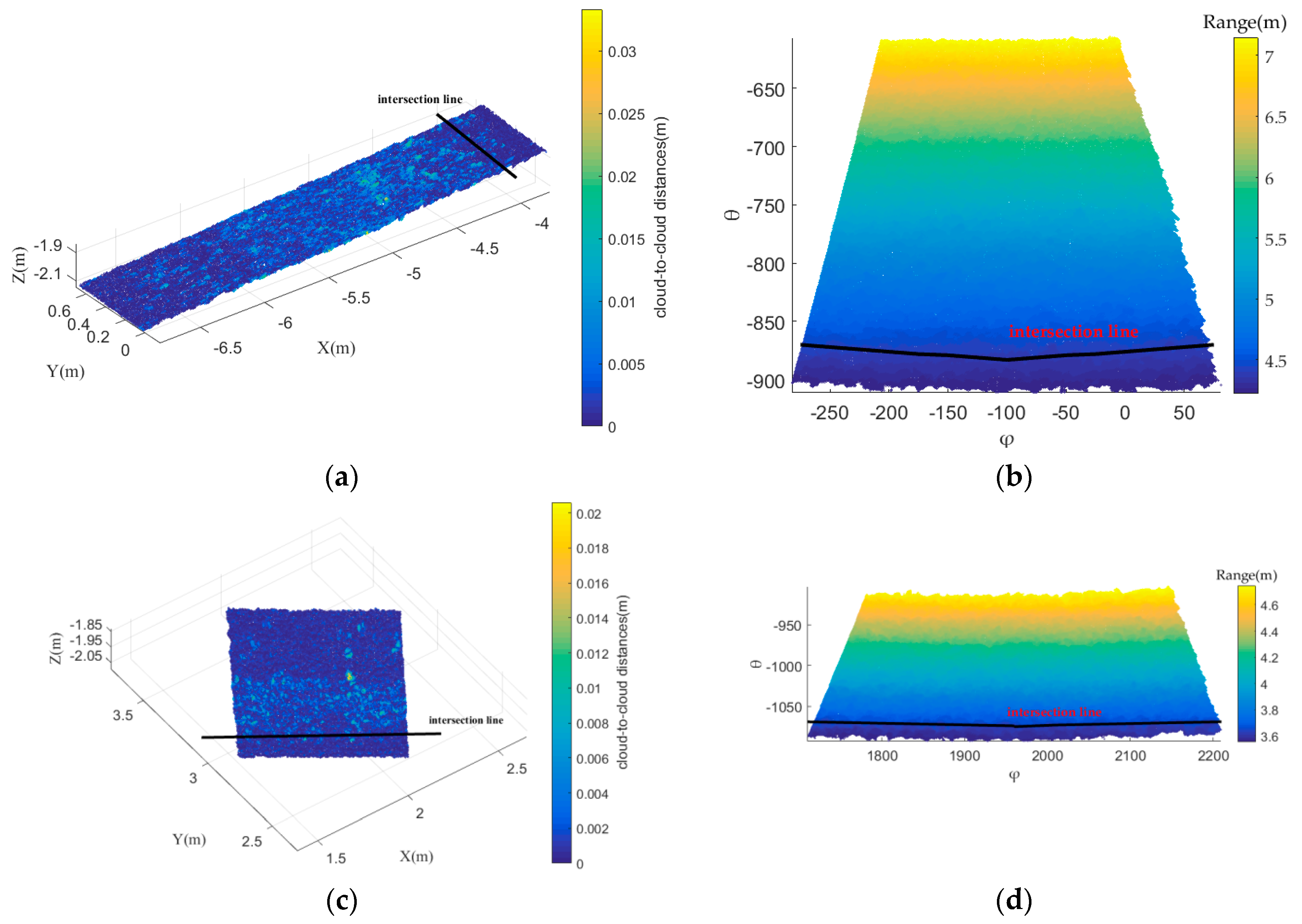
From change analysis results using the cloud-to-cloud distance, it is apparent that the change in the area near the intersection line is larger than in other areas. Therefore, points were selected manually from the global point cloud around this area. The range images were created according to Equation (1) for the two slopes respectively. Figure 8a,c show the raw point cloud colored by cloud-to-cloud distances for Slope 1 and Slope 2, respectively. Figure 8b,d show the range images colored by ranges for Slope 1 and Slope 2, respectively.

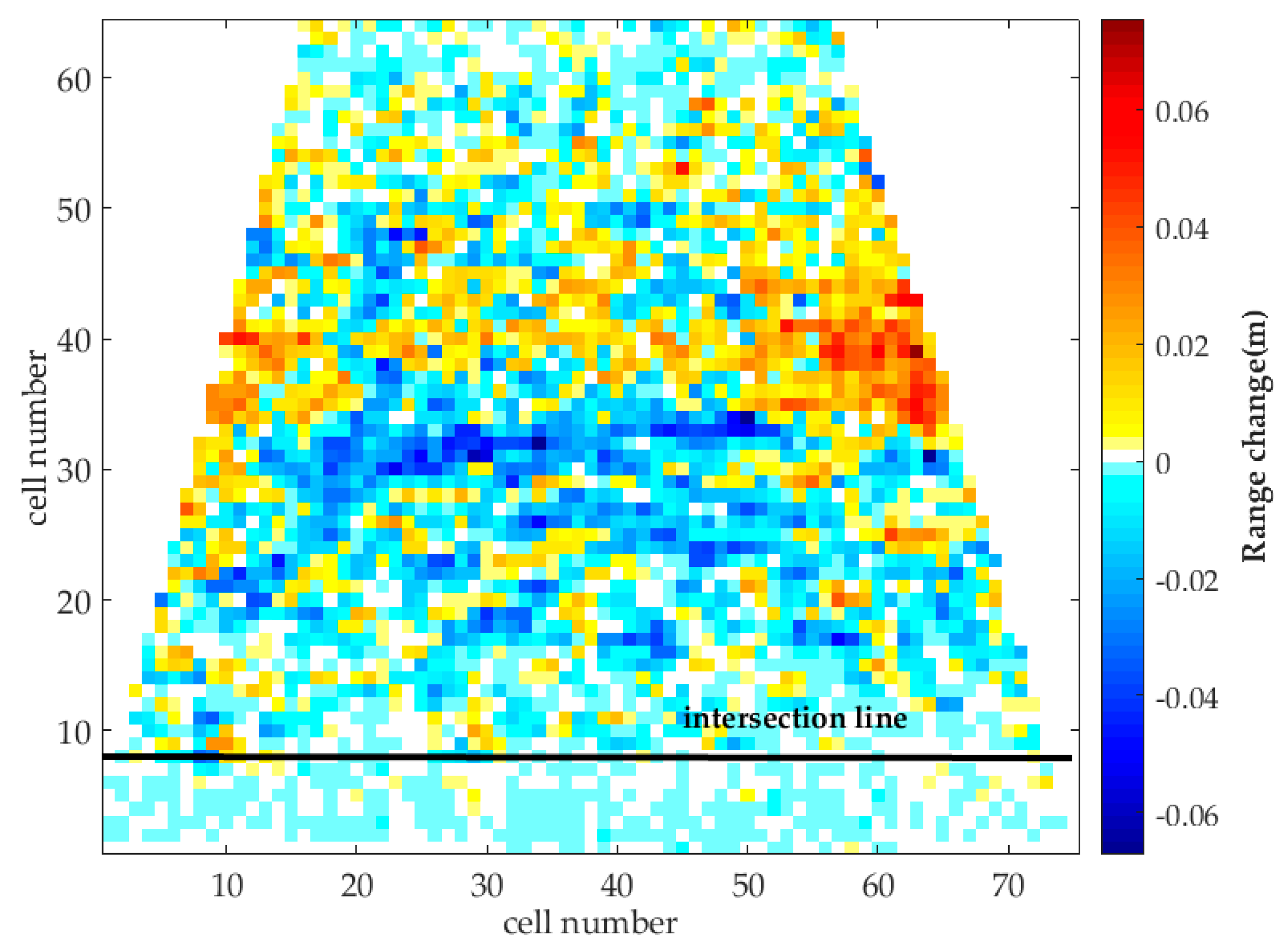
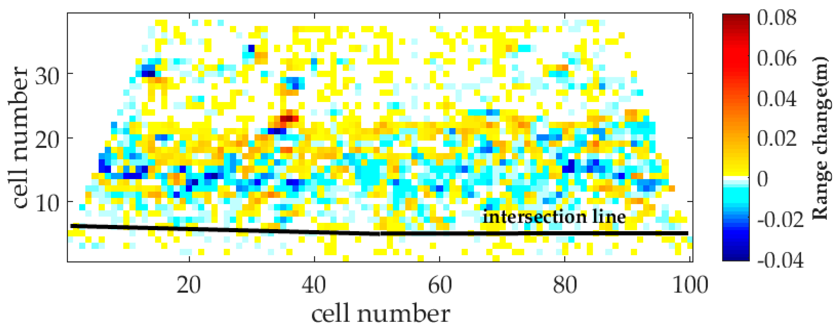
In the range image, the horizontal and vertical axes correspond to the horizontal and vertical scan angles, respectively. In our experiment, the horizontal and vertical angle resolutions are both 0.0005 rad. Here, the size of the image cell was set at 5 times this angular resolution, i.e., at a value of 0.0025 rad, to insure the number of points in each cell is more than 20. Next, the range image was divided into cells of 0.0025 rad × 0.0025 rad. To remove the influence of edge effects, cell creation started from the center of the range image. For each point in a given cell, the mean range was estimated by averaging the ranges of all point within the current cell. Through comparing the corresponding cells in two epochs, the range change was estimated. 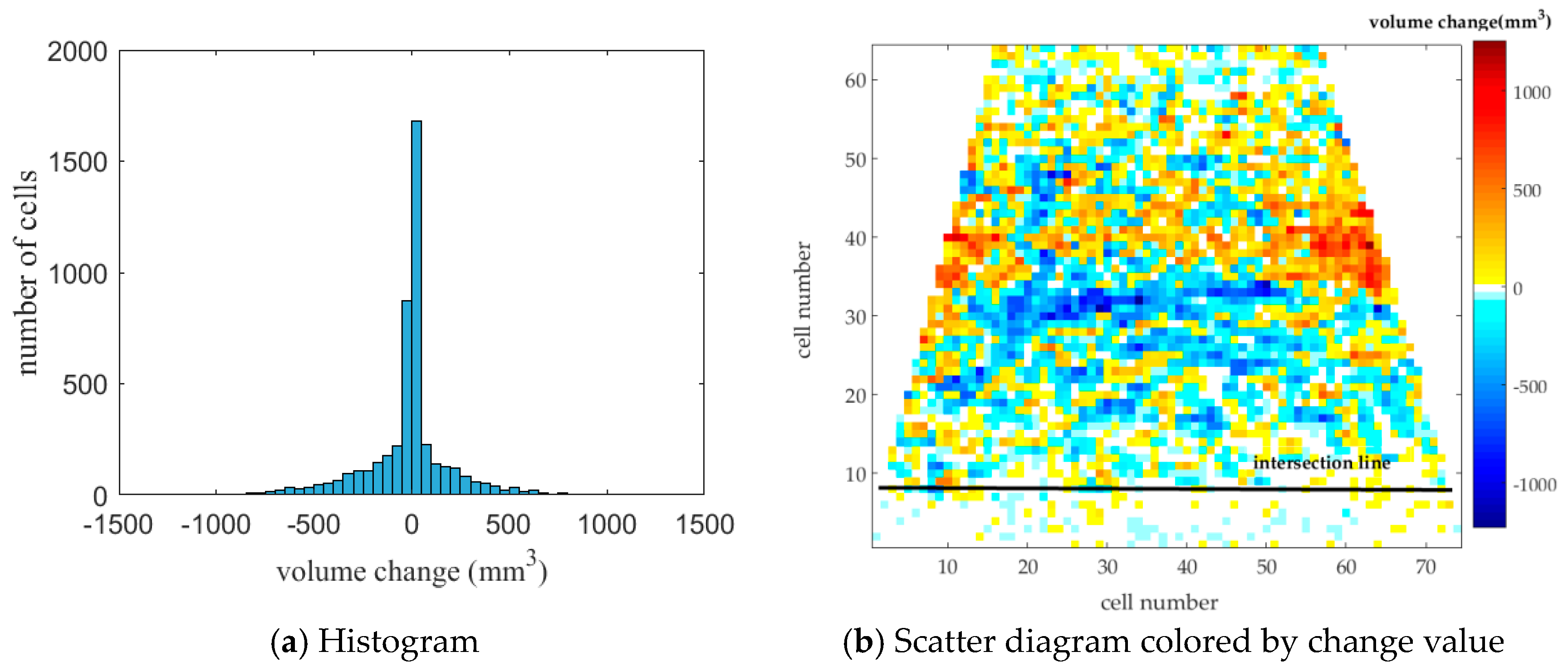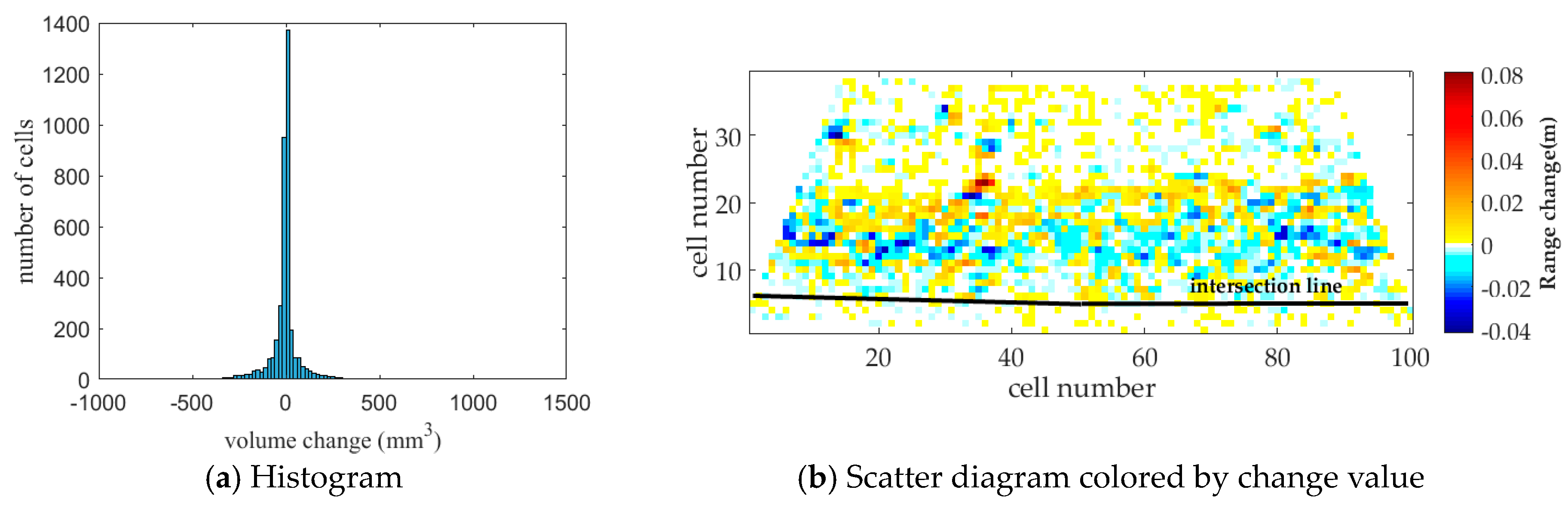The range images colored by range change for Slope 1 and Slope 2 are shown in Figure 9 and Figure 10, respectively. Range changes with negative values indicate rocks in the current cell that have moved closer to the scanner location after the wave attack test. Conversely, the range change with positive values correspond to the rocks in the current cell that moved away from the scanner center after the wave attack test.

For further characterizing the change information, the range change is projected to the directions along and perpendicular to the slope. Based on the horizontal angles, the center of the slope is obtained according to the method introduced in Section 3.3. Afterwards, the vectors representing the main direction ($V_1$) along the slope, the second direction ($V_2$) across the water flume, and the third direction ($V_3$) vertically upwards against the slope plane are estimated. These vectors are summarized in

Table 4. Vectors representing the three main directions for the two slopes.

	Slope 1	Slope 2
$V_1$	[0.9942, −0.0497, 0.0955]	[0.5457, 0.8158, −0.1913]
$V_2$	[0.0292, 0.9995, −0.0082]	[0.8445, −0.5354, −0.0129]
$V_3$	[−0.0950, 0.0110, 0.9952]	[0.1129, 0.1545, 0.9812]

.

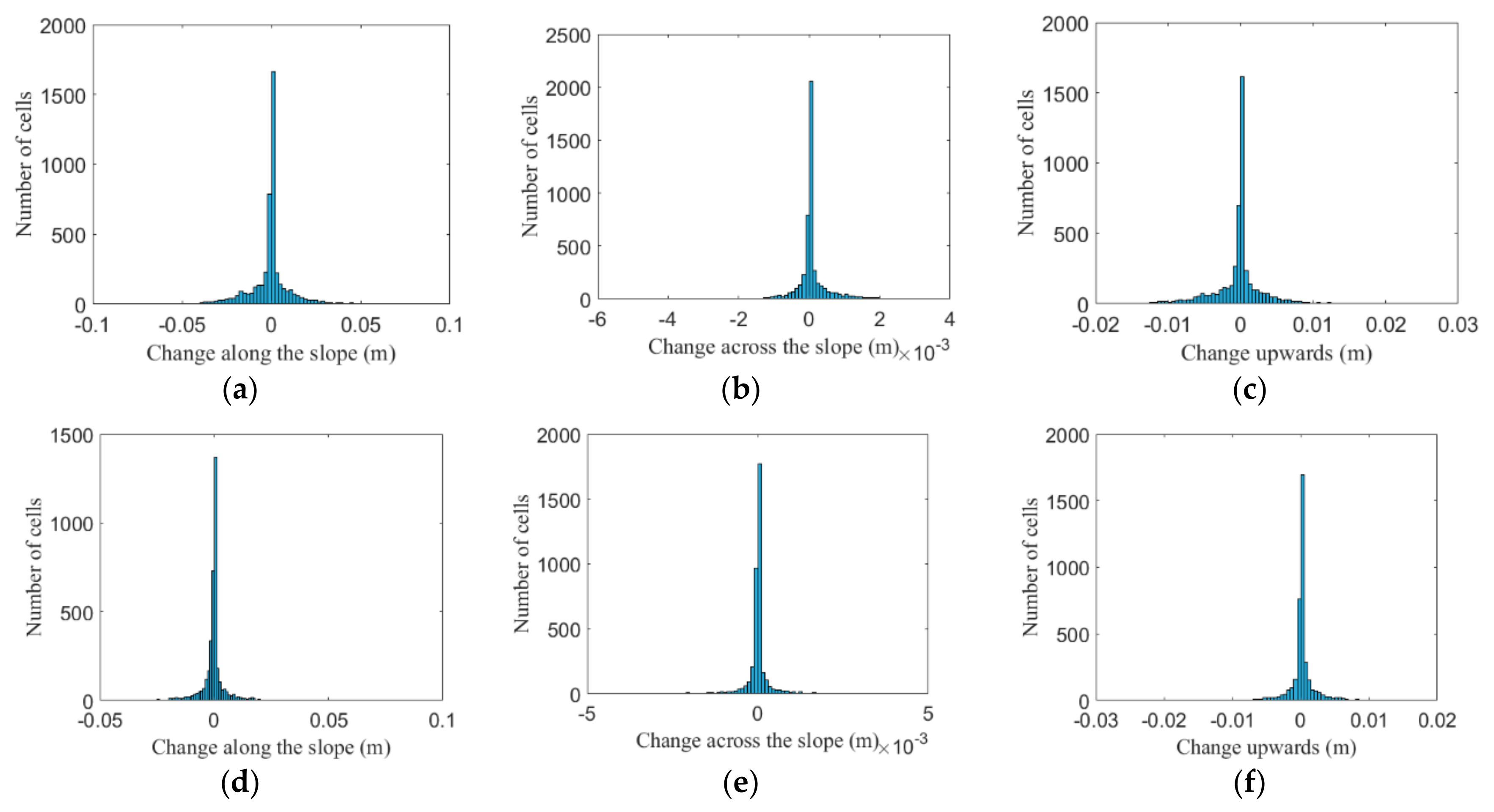
Subsequently, the range change for every cell in the range image is decomposed in the three directions as discussed above. The histograms of the number of cells along slope, across slope, and upwards for Slope 1 are shown in Figure 11a–c, respectively. Similarly, the histograms of the number of cells along slope, across slope, and upwards for Slope 2 are shown in Figure 11d–f, respectively.

As can be seen in Figure 11, the changes for both Slope 1 and Slope 2 in the direction along slope are [−0.0645, 0.0726] m and [−0.0399, 0.0774] m, respectively, with the left value indicating the minimum change while the right value indicates the maximum change values in a slope). The changes for two slopes (Slope 1 and Slope 2) in the direction across the water flume are between [−0.0043, 0.0037] m and [−0.0045, 0.0048] m, respectively. The changes for two slopes (Slope 1 and Slope 2) in the direction vertically upwards against the slope plane are between [−0.0190, 0.0201] m and [−0.0237, 0.0123] m, respectively. Note that the change values in the direction across the water flume have a big difference from the values in the other directions. The absolute change value is relatively small: the minimum value is −0.0043 m and −0.0045 m for Slope 1 and Slope 2, respectively, while the maximum value is 0.0037 m and 0.0048 m. In addition, the cells with an absolute change value less than 0.001 m in the direction across the water flume occupy 92.5% and 95.7% of Slope 1 and Slope 2, respectively. In this regard, considering the registration error, the surface density in different scans, etc., the change in the direction across the water flume can be ignored in the further analysis. 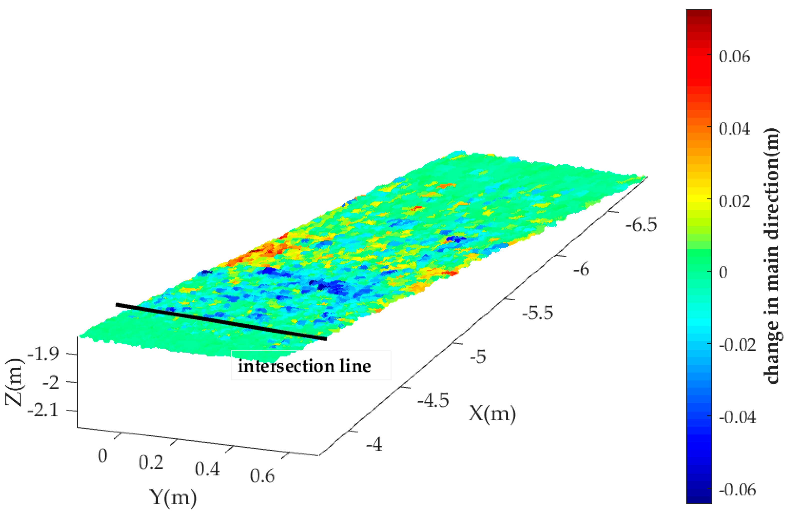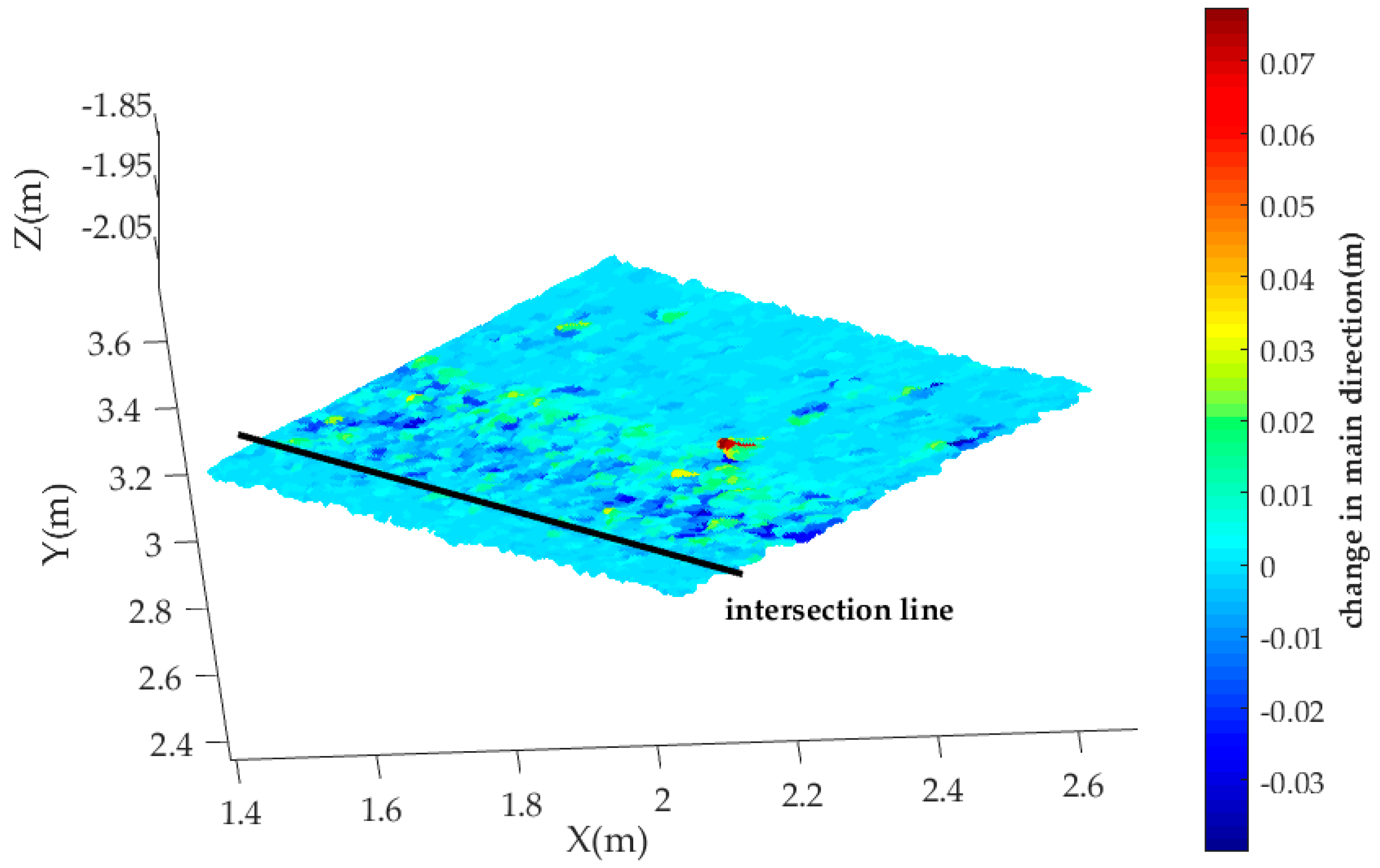Next, the scatter diagrams for the two slopes in the direction along slope are plotted, in Figure 12 and Figure 13.

As shown in Figure 12 and Figure 13, the changes in the direction along slope are symmetrically distributed along the center line of the slope length, i.e., the center line of the water flume. Thus, the change profile along the slope length, i.e., the vertical axis direction ($\phi$) in 2D space, is defined and computed by averaging all the cell values within the same horizontal axis ($\theta$), as in Equation (6):

$$chang(i)=\frac{{\displaystyle \sum _{j-=1}^{n}C\left(i,j\right)}}{n}$$

(6)

where $n$ is the number of columns, in the raster image, and $C\left(i,j\right)$ denotes the change of a raster grid in the i-th row and j-th column.

Figure 14 shows the change profile for the damage area of the two slopes (1:10 and 1:5) in the along slope direction. The maximum and minimum change in the value of direction along the slope for Slope 2 are 0.0052 m and −0.0032 m, respectively, while the same change values for Slope 1 are more significant with values of 0.0121 m and −0.0132 m, respectively. Compared to the change in the direction along the slope, the changes in the direction vertically upwards against the slope plane are less significant, i.e., the maximum change values for Slope 1 and Slope 2 are 0.0036 m and 0.001 m, respectively, and the minimum change values are −0.0036 m and −0.0018 m, respectively. The change information is also summarized in

Table 5. Change information along the slope length.

Slope	Change Direction	Minimum (m)	Maximum (m)
2	along	−0.0032	0.0052
	upwards	−0.0018	0.0010
1	along	−0.0132	0.0121
	upwards	−0.0036	0.0036

.

Close examination of the change information in Figure 14 and Table 5 shows that most change happened at the area around the intersection line. In addition, the changes in the direction along the slope have a similar tendency for Slope 1 and Slope 2, i.e., along the slope, first the change becomes larger, which indicates that some materials (stones) moving to this location from other areas. Then the change becomes smaller which indicates the materials here are moving away after the wave attack test. The slopes tend to be stable away from this location. However, the changes vertically upwards against the slope plane act differently for two slopes. That is, for Slope 1, the change is first larger, then smaller. For Slope 2, the change first is smaller, then larger. This is an interesting phenomenon and the following conclusions can be drawn, (1) For the steeper 1:5 slope, the transport direction changes to be mostly seaward, that is, towards the direction away from the scanner and (2) for the less steep 1:10 slope, the transport is in the opposite direction, that is, towards the direction close to the scanner.

In our previous work [55], we analyzed the same datasets for the slopes but performed another approach consisting of exploiting a slope coordinate system, coordinate transformation, range image creation, change detection, etc. Through comparing the results, we found that the results acquired by the approach proposed in this article correspond well to the results presented in our previous contribution [55] including the change values, change tendency, etc.

3.4. Volume Change Estimation Results

After obtaining the range change for the area of interest, volume change detection is performed according to the method introduced in Section 2.2.4. Figure 15a,b show the histogram and scatter diagram of volume change for Slope 1 while Figure 16a,b show the histogram and scatter diagram of volume change for Slope 2. The maximum volume change, i.e., erosion that occurred for Slope 1 and Slope 2 are 1257.1 mm³ and 1004.8 mm³, respectively. The minimum volume change, i.e., dilation that occurred for Slope 1 and Slope 2 are 1229.8 mm³ and 528.5 mm³, respectively. By summing all the cells in the analyzed area, the total volume changes are estimated with the values of −79,060.9 mm³ and −22,552.2 mm³ for Slope 1 and Slope 2, respectively. It is evident that the volume change in Slope 1 is greater than the volume change in Slope 2. This partly reveals that the influence induced by the wave attack to Slope 1 is greater than to Slope 2, which caused by the different wave conditions, i.e., the wave height applied to slope 1 (0.129 m) was larger than the one that was used for slope 2 (0.054 m).

3.5. Limitation Analysis

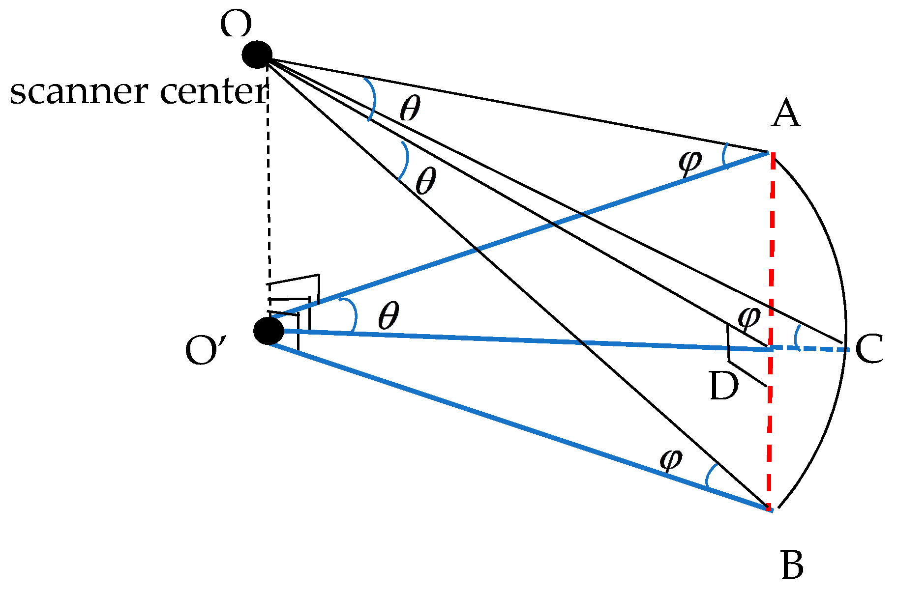
In this study, the rock slopes considered are long and narrow which ensures the excellent performance of the range image technique. However, the width of the slope influences the change profile along the slope length generation. The typical graphical illustration of the scanning is described in Figure 17 where $O$ denotes the scanner center and $O^{\prime }$ denotes the scanner center projection in the slope plane. The slope length direction is represented by $O^{\prime }C$, the points in the arc $ACB$ are with identical vertical angle so they are expected to have the same vertical coordinates in 2D space that are revealed by a line. In reality, the points in the line $AB$ across the slope are expected to be extracted rather than the point in the arc $ACB$. This somehow causes errors in generating the change profile along the slope length. Assuming that the distance from $O^{\prime }$ to $D$ in the slope plane is $\Vert O^{\prime }D\Vert$ with a value of $L_1$, the distance from the scanner center to the slope plane is $\Vert O{O}^{\prime }\Vert$ with a value of $H$, the vertical angle at current position is $\phi$, the angle between $OA$ and $OD$ is $\theta$, and the width of the slope ($AB$) is $W_1$, thus,

$$\Vert AD\Vert =\frac{W_1}{2}$$

(7)

$$\theta =\arctan \left(\frac{\Vert AD\Vert }{\Vert O^{\prime }D\Vert }\right)$$

(8)

$$\Vert O^{\prime }A\Vert =\sqrt{{\Vert O^{\prime }D\Vert }^2+{\Vert AD\Vert }^2}$$

(9)

$$\phi =\arctan \left(\frac{\Vert O{O}^{\prime }\Vert }{\Vert O^{\prime }A\Vert }\right)$$

(10)

$$\Vert O^{\prime }C\Vert =\frac{\Vert O{O}^{\prime }\Vert }{\tan \phi }$$

(11)

Finally, the distance between $C$ and $D$ is estimated by $\Vert O^{\prime }D\Vert -\Vert O^{\prime }C\Vert$.

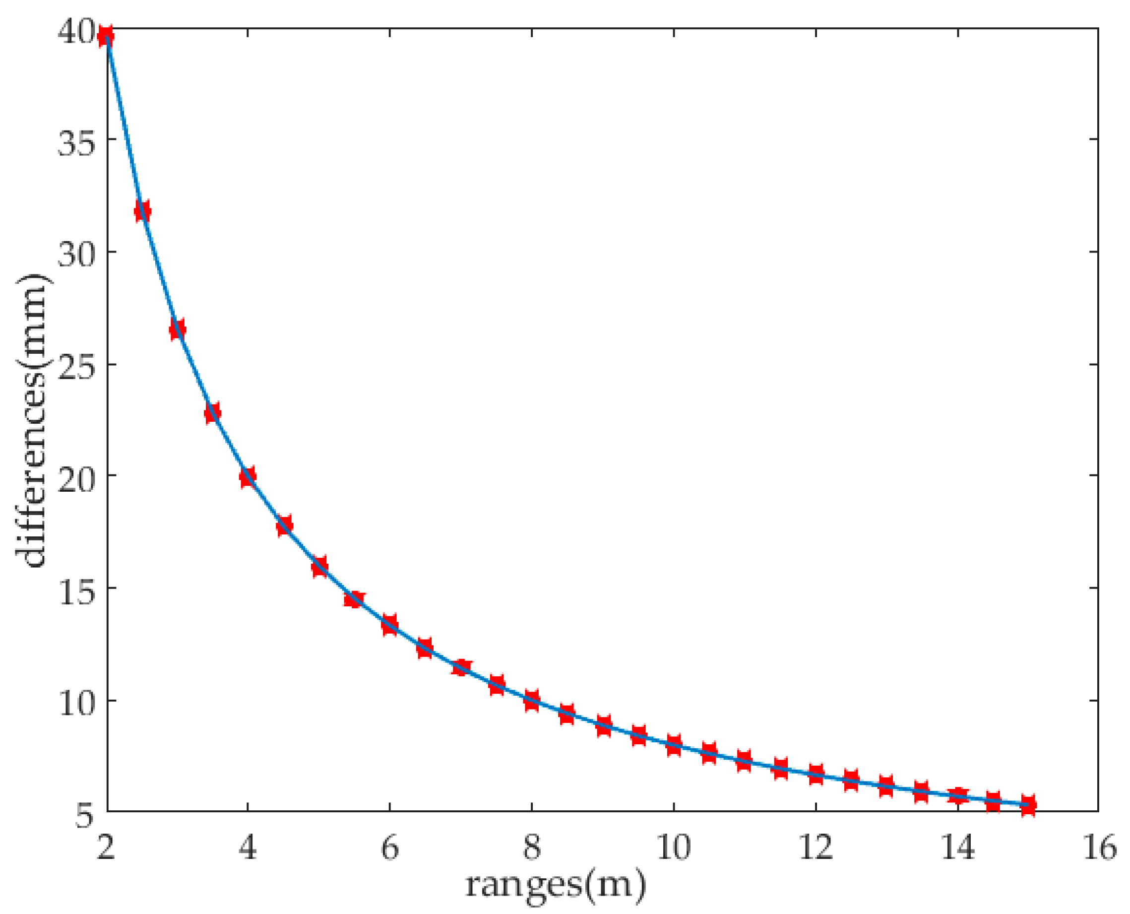
In our experiment, the width of the slope is 0.8 m, the range for Slope 1 is less than 9 m while for Slope 2 it is less than 15 m. The distance from the scanner center to the slope plane is less than 2 m. Here we define the distance $\Vert O{O}^{\prime }\Vert$ equals to 2 m, and the range of 2 m to 15 m is used to illustrate the influence induced by the range image technique. A graph indicating the difference ($\Vert CD\Vert$) against the ranges is shown in Figure 18. It is apparently that the difference decreases as the range increase. The difference at the range of 2 m is 0.0396 m while the difference at the range of 15 m is 0.0053 m. Considering the absolute value is with a relatively small magnitude, the difference that shifting in the direction along the slope length induced by the method is acceptable. In this sense, the method presented here can be applied to any object with similar characteristics with the rock slopes of narrow and long dimensions, e.g., metro tunnels, railways, highways, and large-scale bridges. The above-analysis indicates the main limitation of range image technique applied in the change analysis of rock slopes. However, it definitely has no influence on the cell change analysis, volume change estimation, etc.

In order to investigate the influence induced by various point density on the volume change estimation results, the raw point clouds were downsampled with the percentage of 50%, 25%, and 10%, respectively. The surface density of slope 1 for the raw, 50%, 25%, and 10% of the point clouds is 378,089 pt/m², 189,044 pt/m², 94,522 pt/m², and 37,809 pt/m², respectively. While the corresponding surface density for slope 2 is 577,888 pt/m², 288,944 pt/m², 144,472 pt/m², and 57,789 pt/m², respectively. The proposed methodology was implemented on the downsampled point clouds again; the volume change information for the four cases are summarized in

Table 6. Comparison of the volume changes for the raw and downsampled point clouds (units: m mm³).

Point Clouds	Maximum		Minimum		Mean		Sum
	Slope 1	Slope 2	Slope 1	Slope 2	Slope 1	Slope 2	Slope 1	Slope 2
raw	1257.1	1004.8	−1229.8	−528.5	−16.7	−5.9	−79,060.9	−22,552.2
50%	1261.9	1003.3	−1194.2	−540.7	−16.1	−5.5	−76,013.7	−20,976.4
25%	1192.0	994.4	−1262.5	−546.4	−18.4	−5.8	−86,922.1	−22,011.8
10%	1506.9	991.4	−1408.7	−486.9	−17.2	−7.3	−81,596.1	−27,669.2

. The maximum volume changes for erosion occurred, extracted from the raw, 50%, 25%, and 10% of point clouds for slope 1 are 1257.1 mm³, 1261.9 mm³, 1192.0 mm³, and 1506.9 mm³, respectively. While for slope 2 the maximum volume changes are 1004.8 mm³, 1003.3 mm³, 994.4 mm³, and 991.7 mm³, respectively. The minimum volume changes, i.e., dilation occurred, extracted from the raw, 50%, 25%, and 10% of point clouds for slope 1 are −1229.8 mm³, −1194.2 mm³, −1262.5 mm³, and −1408.7 mm³, respectively, in which the symbol “−” represents the dilation occurred. While for slope 2 the minimum volume changes are −528.5 mm³, −540.7 mm³, −546.4 mm³, and −486.9 mm³, respectively. Afterwards, the volume changes for the entire damaged area were estimated with values of −79,060.9 mm³, −76,013.8 mm³, −86,922.1 mm³, and −81,596.1 mm³, for the raw, 50%, 25%, and 10% of the point clouds, respectively. Next, the comparison of the extracted volume change results between the downsampled point clouds and the raw point cloud was carried out. It is evident that the maximum and minimum volume changes have a relatively large difference for the downsampled point cloud of 10% w.r.t the raw point cloud. In the case of the downsampled point cloud of 10%, the average point space is ~5.2 mm, namely on the surface of one stone (nominal diameter is 16.20 mm), the number of points is less than ten, so the points are not enough for reflecting the stone surface in an accurate way. Therefore, the low point density influences the extraction results of the volume change. In this regard, we conclude that relatively ideal volume change estimation results could be obtained under the surface point density greater than 144,472 pt/m².

To investigate the influence induced by various cell sizes on the volume change estimation results, the raster image is divided into cells of 0.01 rad × 0.01 rad, 0.005 rad × 0.005 rad, and 0.001 rad × 0.001 rad, respectively, for volume change estimation. The results are summarized in

Table 7. Comparison of the volume changes for various cell sizes (units: mm³).

Cell Size (rad)	Maximum		Minimum		Mean		Sum
	Slope 1	Slope 2	Slope 1	Slope 2	Slope 1	Slope 2	Slope 1	Slope 2
0.01 × 0.01	748.0	2683.7	−507.6	−4309.9	−10.8	−117.8	−3123.1	−29,440.3
0.005 × 0.005	1008.5	2615.9	−832.1	−1413.4	−16.6	−23.6	−19,673.7	−23,144.4
0.0025 × 0.0025	1257.1	1004.8	−1229.8	−528.5	−16.7	−5.9	−79,060.9	−22,552.2
0.001 × 0.001	1169.3	196.8	−1555.4	−138.3	−28.5	−0.9	−135,040.3	−21,047.1

(results of cell of 0.0025 rad × 0.0025 rad included). Thanks to the various cell sizes, it is reasonable that the maximum, minimum, and mean volume changes are different against the various cell sizes. The volume changes of the entire interest area, i.e., the sum of the volume changes w.r.t four cell sizes are expected to be identical. However, as shown in Figure 7, we found that for slope 1, the sum of the volume change becomes smaller with increased cell size, namely, the greater the cell size the smaller the sum of the volume change. While for slope 2, the sum of the volume change for the cell sizes of 0.01 rad × 0.01 rad, 0.005 rad × 0.005 rad, 0.0025 rad × 0.0025 rad, and 0.001 rad × 0.001 rad are −29,440.3 mm³, −23,144.4 mm³, −22,552.2 mm³, and −21,047.1 mm³, respectively, and their magnitudes are almost the same. As shown in Section 3.2, the mean distance from the damaged area to the scanner center for slope 1 is ~6.2 m; while the value for slope 2 is ~4.17 m. Therefore, for the raster image of slope 1 with the cell sizes of 0.001 rad × 0.001 rad, 0.0025 rad × 0.0025 rad, 0.005 rad × 0.005 rad, and 0.01 rad × 0.01 rad, the corresponding cell sizes in Euler space are ~0.006 m, ~0.015 m, ~0.03 m, and ~0.06 m, respectively. For the raster image of Slope 2 with the cell sizes of 0.001 rad × 0.001 rad, 0.0025 rad × 0.0025 rad, 0.005 rad × 0.005, rad and 0.01 rad × 0.01 rad, the corresponding cell sizes in Euler space are ~0.004 m, ~0.01 m, ~0.02 m, and ~0.04 m. At this point, we found that if the cell size in Euler space is greater than the nominal of the stone diameter, i.e., 16.2 mm, one cell covers more than one complete stone which causes the accretion or the erosion of the current cell averaged by the region outside the stone. In this regard, the effectiveness and reliable of the proposed methodology is constrained by the cell size, that is, it is better to set the cell size smaller than the nominal size of the particles composing the slopes in the real applications.

As stated in a past paper [64], terrestrial laser scanning measurements are subject to noise induced from the incident angle. They concluded that above a 60 degree incidence angle, noise in the measurements affect the scan point precision. In our experiment, the incidence angle is close to 60 degrees, even greater than 60 degrees in some areas. However, considering the distinctiveness of the rock slope with the characteristics of long and narrow, it is unavoidable to guarantee the incident angles w.r.t entire areas greater than 60 degrees. As a result, we only used the damaged area that is close to the scanner center, i.e., the incidence angle is relatively small w.r.t the entire slope, for change analysis. This setting somehow improved the reliability of the volume change extraction results. Moreover, the raster image was introduced in this article which averaged all points in each cell. This step also reduced the error induced by the incidence angle. In the real application, it is better to mount the scanner with a relatively higher position with respect to the object to ensure a smaller incident angle which definitely increases the feasible and accuracy of the proposed methodology.

Also, the roughness of the slope is another factor that influences the plausibility of the proposed methodology. In our experiment, all the stones composing the slope are clear and have almost identical size, i.e., they have relatively low roughness. However, in the real application, the particles composing the slopes are dirty, e.g., with impurities, vegetation that grew around it and lichen, irregular in different areas. This maybe result in the roughness in different areas varies greatly, and then somehow influence the accuracy of the volume change estimation results. Therefore, an additional step is to assess the roughness of the object surface before implementing the proposed methodology. Several roughness assessment methods have been proposed, e.g., in multiple past papers [65,66], based on of which the raw point cloud could be cleared.

4. Discussion

The results obtained in Section 3.1, Section 3.2, Section 3.3, Section 3.4 and Section 3.5 show that the proposed methodology presented here is efficient and feasible. In this section, we emphasize the advantages of our approach, but also the practical challenges faced.

One of the main advantages of the method is the reduction of computational costs in an accurate way. In the conventional approach, as reported in a past paper [55], several additional processes, e.g., normal vector estimation, were required that had to executed on the full point cloud, before a suitable coordinate transformation could be estimated. The accuracy of these processing steps was affected by data noise, edge effects, variation in surface density, etc. In contrast, the range image technique, which is a 2.5D approach, enables the user to lift geometrical information back from 2D raster space to 3D space. This workflow, from 3D point cloud to 2D raster and back to 3D point cloud, ensures the directions of interest are easy and can be reliably estimated in 2D space. Besides, in a traditional Cartesian raster image based on coordinates transformation, cell sizes in 3D space are almost the same but the number of points in each cell varies with the local point density which depends on the measurement geometry. In the raster image approach, as discussed in this paper, the number of points in each 2D cell is almost identical which guarantees a certain uniformity of point cloud quality and accuracy.

The workflow in this research considered a specific indoor scene. Still, a similar workflow can and will also be applied in large outdoor coastal scenarios. For example, in [67], a so-called permanent laser scanning setup is discussed, in which the same sandy beach is scanned over and over again at hourly intervals for a total period of, for example, 6 months. To detect changes in such a spatiotemporal data set, similar methodology as presented in this paper will be applied. As scanning always takes place from the same location, only a fine registration procedure is needed to align scans from different epochs. Next, data of each epoch will be organized in an aspherical coordinate system as discussed in this research. Such organization will enable to handle the larger point clouds efficiently as neighbor detection can exploit the 2D grid organization, while the grid size can be adapted to size of the changes to be detected.

This methodology is notably suitable if scan data from one scan position is compared. Even if more scan positions are considered, a similar approach can be used, as already demonstrated by Zeibak and Filin in [68], where a second viewpoint is transformed to match a scan from a first viewpoint in a methodology that distinguishes areas that were changes from areas that are either stable or occluded because of the difference in viewpoints.

The change analysis results clearly indicate that the damage happened in the area near the intersection line between the wave surface and the slope plane. By predefining the size of the cells, we generated the raster image based on the range image technique to easily quantify the changes. Consequently, we performed the quantification and estimation of changes, which showed favorable results for detecting changes from rock slopes subject to wave attack test. To this end, the volume change estimation is done to validate the results. The results show that the transport direction actually swaps from seaward, for steeper 1:5 slope, to landward, for the less steep 1:10 slope. To this end, the limitation of the range image technique applied in change analysis of rock slopes is reported that related to the shifting in the direction along slope. Even so, after performing the range image technique, the computational performance is actually enhanced.

The methodology presented herein is of great practical importance for engineers involved in coastal zone management, coastal zone policy makers, etc., providing them guidance for the application of TLS in the evaluation of rock slopes. Specifically, the results about the transport direction of rock slopes with different steepness can serve to learn to understand the physical processes and can be further translated into governing practical engineering parameters, such as the selection of steepness for designing the coastal structures, damage evaluation, etc. Also, the possibility and effectiveness of the stones used in our experiment are verified. Furthermore, it has been proven that the laser scanning technique for understanding the motion of rock slopes can be extended to the change detection of coastal protection structures composing of stones.

However, for real applications, some problems need to be solved. First, in real scenarios such as shore lines, the region of interest is not necessarily narrow; the initial point cloud should be first subdivided into smaller clouds along the shore line with a defined width so that each partial cloud can be inspected for changes. A second problem could be the lack of identifiable points for TCP matching between two scans. Some stable artificial objects, e.g., mobile signal towers or corner of the buildings, could be used for registration between two scans.

5. Conclusions

The methodology proposed herein is an efficient and precise means of detecting changes from rock slopes using dense terrestrial laser scanning point clouds, providing a new way to evaluate the erosion of rock slopes to wave attack in coastal engineering. The estimation of erosion or dilation is a new possibility with the range image technique due to its large spatial resolution. In our case studies, the results are encouraging. The use of dense terrestrial laser scanning point cloud can provide information about the stone motion in the rock slopes more efficiently and at a higher resolution compared to classical instruments.

The processing of dense terrestrial laser scanning point cloud for change analysis presented in this article includes registration using TCP method, change detection using the cloud-to-cloud distances, range image generating based on the horizontal and vertical angular resolution, raster image creation, quantification of changes, and volume change estimation. During scanning, three plane targets were set between two scans before and after the wave attack test, a high precision registration was performed with the registration error less than 1 mm. The cloud-to-cloud distances were first adopted to realize the direct point cloud comparison, so that the damage area with significant change value was recognized. However, the notation of this type of distance is always positive that means it only purely reflects the magnitude of the change and the direction of the change is beyond expression. In such a case, for obtaining the magnitude and direction of the change, the range image technique was introduced. Based on the horizontal and vertical angular resolution given by the scanner itself, the transformation from 3D Cartesian coordinates to 2D range image is determined. For easier for quantification of changes, the raster image based on the range image technique was generated by predefining a cell size. As a result, the quantification and estimation of changes were performed and favorable results were also obtained for detecting changes from rock slopes subject to wave attack test.

The main contribution of this article focuses on the introduced range image technique for the change analysis of rock slopes with the characteristics of long and narrow, the limitations of which have been summarized in Section 3.5. However, from the perspective of the technique itself, it is really a promising approach for change analysis the long and narrow objects which somehow avoid introducing the unalignment error. Meanwhile, the identical number of points in different cells enables the equal-accuracy analysis which is a vital factor for the global analysis of the objects.

However, in our study, only two types of slopes were tested and analyzed, for insight into the influence induced by the various steepness, more types of steepness of slopes should be considered and implemented to obtain more information about the stability of slopes within various steepness. Meanwhile, more types of stones should be tested to find the optimal size of stone at a given steepness. In addition, due to the change that mostly happened near the intersection line, we believe that the change value is related the distance between the stone surface and the wave surface. However, we did not focus on this point in this paper which may be an interesting topic in the further study, the goal of which is to establish a rigorous mathematical model between the change value and the distance.

Upcoming research will focus on more detailed change information extraction such as each individual stone shape extraction and interpretation. However, it definitely a hard task from a laser scanning processing perspective due to the reasons such as the shape of the stone is irregular, it is difficult to acquire the point cloud for an entire stone, various point densities, etc. In reality, the movement of individual stones under wave attack is constrained in certain ways by gravity, wave forces, and friction between rocks; the motion can be regarded as a random process. For better understanding the change of the slope and the movement of individual stone, gravimetric analysis of each stone, friction analysis between stones, wave forces on the stones, and other possible influence factors are required. It is an interesting topic in the fields of surveying, remote sensing, coastal engineering, and hydraulic engineering.

References

1. Nicholson-Cole, S.A. Representing climate change futures: A critique on the use of images for visual communication. Comput. Environ. Urban Syst. 2005, 29, 255–273. [Google Scholar] [CrossRef]
2. Hanley, M.E.; Hoggart, S.P.G.; Simmonds, D.J.; Bichot, A.; Colangelo, M.A.; Bozzeda, F.; Heurtefeux, H.; Ondiviela, B.; Ostrowski, R.; Recio, M. Shifting sands? Coastal protection by sand banks, beaches and dunes. Coast. Eng. 2014, 87, 136–146. [Google Scholar] [CrossRef]
3. Emery, S.M.; Rudgers, J.A. Ecological assessment of dune restorations in the great lakes region. Restor. Ecol. 2010, 18, 184–194. [Google Scholar] [CrossRef]
4. Ferdos, F.; Wörman, A.; Ekström, I. Hydraulic conductivity of coarse rockfill used in hydraulic structures. Transp. Porous Media 2015, 108, 367–391. [Google Scholar] [CrossRef]
5. Rijn, L.C.V. Coastal erosion and control. Ocean Coast. Manag. 2011, 54, 867–887. [Google Scholar] [CrossRef]
6. Javadi, N.; Mahdi, T.F. Experimental investigation into rockfill dam failure initiation by overtopping. Nat. Hazards 2014, 74, 623–637. [Google Scholar] [CrossRef]
7. Morán, R.; Toledo, M.Á. Research into protection of rockfill dams from overtopping using rockfill downstream toes. Revue Canadienne de Génie Civil 2011, 38, 1314–1326. [Google Scholar]
8. Landry, C.E.; Keeler, A.G.; Kriesel, W. An economic evaluation of beach erosion management alternatives. Mar. Resour. Econ. 2003, 18, 105–127. [Google Scholar] [CrossRef]
9. Firth, L.; Thompson, R.; Bohn, K.; Abbiati, M.; Airoldi, L.; Bouma, T.; Bozzeda, F.; Ceccherelli, V.; Colangelo, M.; Evans, A. Between a rock and a hard place: Environmental and engineering considerations when designing coastal defence structures. Coast. Eng. 2014, 87, 122–135. [Google Scholar] [CrossRef] [Green Version]
10. Van Der Meer, J.W. Rock Slopes and Gravel Beaches under Wave Attack; Delft Hydraulics: Delft, The Netherlands, 1988; Volume 396. [Google Scholar]
11. Thompson, D.; Shuttler, R. Riprap design for wind wave attack. In A Laboratory Study in Random Waves; HR Wallingford: London, UK, 1975. [Google Scholar]
12. Van der Meer, J.W.; Stam, C.-J.M. Wave runup on smooth and rock slopes of coastal structures. J. Waterw. Port Coast. Ocean Eng. 1992, 118, 534–550. [Google Scholar] [CrossRef]
13. Smith, W.G.; Kobayashi, N.; Kaku, S. Profile changes of rock slopes by irregular waves. In Proceedings of the Coastal Engineering, Venice, Italy, 4–9 October 1992; pp. 1559–1572. [Google Scholar]
14. Allison, R.J.; Kimber, O.G. Modelling failure mechanisms to explain rock slope change along the isle of purbeck coast, UK. Earth Surf. Process. Landf. 1998, 23, 731–750. [Google Scholar] [CrossRef]
15. Jaboyedoff, M.; Metzger, R.; Oppikofer, T.; Couture, R.; Derron, M.; Locat, J.; Turmel, D. New insight techniques to analyze rock-slope relief using dem and 3d-imaging cloud points: Coltop-3d software. In Rock Mechanics: Meeting Society’s Challenges and Demands; CRC Press: Boca Raton, FL, USA, 2007; pp. 61–68. [Google Scholar]
16. Salvini, R.; Francioni, M.; Riccucci, S. The accuracy assessment of geomatics data used in rock slope stability analysis. In Proceedings of the European Congress on Regional Geoscientific Cartography and Information Systems, Bologna, Italy, 12–15 June 2012; pp. 105–106. [Google Scholar]
17. Hofland, B.; Gent, M.V.; Raaijmakers, T.; Liefhebber, F. Damage evaluation using the damage depth. In Coastal Structures 2011: (in 2 Volumes); World Scientific: Singapore, 2013; pp. 812–823. [Google Scholar]
18. Hofland, B.; Disco, M.; Van Gent, M. Damage characterization of rubble mound roundheads. In Proceedings of the CoastLab2014, Varna, Bulgaria, 29 September 2014. [Google Scholar]
19. Raaijmakers, T.; Liefhebber, F.; Hofland, B.; Meys, P. Mapping of 3d-bathymetries and structures using stereophotography through an air-water-interface. Coastlab 2012, 12, 17–20. [Google Scholar]
20. Tulsi, K.R. Three Dimensional Method for Monitoring Damage to Dolos Breakwaters. Ph.D. Thesis, Stellenbosch University, Stellenbosch, South Africa, 2016. [Google Scholar]
21. Gent, M.R.A.V. Oblique wave attack on rubble mound breakwaters. Coast. Eng. 2014, 88, 43–54. [Google Scholar] [CrossRef]
22. Maciñeira, E.G.; Burcharth, H.F. Stability of cube armoured roundheads exposed to long crested and short crested waves. Coast. Eng. 2016, 112, 99–112. [Google Scholar] [CrossRef]
23. Vosselman, G.; Maas, H.-G. Airborne and Terrestrial Laser Scanning; Whittles Publishing: Dunbeath, UK, 2010. [Google Scholar]
24. Shen, Y.; Lindenbergh, R.; Wang, J. Change analysis in structural laser scanning point clouds: The baseline method. Sensors 2017, 17, 26. [Google Scholar] [CrossRef] [PubMed]
25. Nuttens, T.; Wulf, A.D.; Deruyter, G.; Stal, C.; Backer, H.D.; Schotte, K. Application of laser scanning for deformation measurements: A comparison between different types of scanning instruments. In Proceedings of the FIG Working Week: Knowing to Manage the Territory, Protect the Environment, Evaluate the Cultural Heritage, Rome, Italy, 6–10 May 2012; pp. 1–13. [Google Scholar]
26. Pesci, A.; Teza, G.; Bonali, E. Terrestrial laser scanner resolution: Numerical simulations and experiments on spatial sampling optimization. Remote Sens. 2011, 3, 167–184. [Google Scholar] [CrossRef]
27. Kang, Z.; Zhang, L.; Lei, T.; Wang, B.; Chen, J. Continuous extraction of subway tunnel cross sections based? On terrestrial point clouds. Remote Sens. 2014, 6, 857–879. [Google Scholar] [CrossRef]
28. Zhao, X.; Kargoll, B.; Omidalizarandi, M.; Xu, X.; Alkhatib, H. Model selection for parametric surfaces approximating 3d point clouds for deformation analysis. Remote Sens. 2018, 10, 634. [Google Scholar] [CrossRef]
29. Kromer, R.A.; Abellán, A.; Hutchinson, D.J.; Lato, M.; Edwards, T.; Jaboyedoff, M. A 4d filtering and calibration technique for small-scale point cloud change detection with a terrestrial laser scanner. Remote Sens. 2015, 7, 13029–13052. [Google Scholar] [CrossRef]
30. Barnhart, T.B.; Crosby, B.T. Comparing two methods of surface change detection on an evolving thermokarst using high-temporal-frequency terrestrial laser scanning, selawik river, alaska. Remote Sens. 2013, 5, 2813–2837. [Google Scholar] [CrossRef]
31. Janowski, A.; Nagrodzka-Godycka, K.; Szulwic, J.; Ziółkowski, P. Remote sensing and photogrammetry techniques in diagnostics of concrete structures. Comput. Concr. 2016, 18, 405–420. [Google Scholar] [CrossRef]
32. Lichti, D.D. A review of geometric models and self-calibration methods for terrestrial laser scanners. Boletim de Ciencias Geodesicas 2010, 16, 3–19. [Google Scholar]
33. Pingue, F.; Petrazzuoli, S.M.; Obrizzo, F.; Tammaro, U.; Martino, P.D.; Zuccaro, G. Monitoring system of buildings with high vulnerability in presence of slow ground deformations (The Campi Flegrei, Italy, case). Measurement 2011, 44, 1628–1644. [Google Scholar] [CrossRef]
34. Capra, A.; Bertacchini, E.; Castagnetti, C.; Rivola, R.; Dubbini, M. Recent approaches in geodesy and geomatics for structures monitoring. Rendiconti Lincei 2015, 26, 53–61. [Google Scholar] [CrossRef] [Green Version]
35. Ghuffar, S.; Székely, B.; Roncat, A.; Pfeifer, N. Landslide displacement monitoring using 3d range flow on airborne and terrestrial lidar data. Remote Sens. 2013, 5, 2720–2745. [Google Scholar] [CrossRef]
36. Qiao, G.; Lu, P.; Scaioni, M.; Xu, S.; Tong, X.; Feng, T.; Wu, H.; Chen, W.; Tian, Y.; Wang, W. Landslide investigation with remote sensing and sensor network: From susceptibility mapping and scaled-down simulation towards in situ sensor network design. Remote Sens. 2013, 5, 4319–4346. [Google Scholar] [CrossRef]
37. Jankowski, R.; Wilde, K.; Fujino, Y. Pounding of superstructure segments in isolated elevated bridge during earthquakes. Earthq. Eng. Struct. Dyn. 2015, 27, 487–502. [Google Scholar] [CrossRef]
38. Chow, J.; Lichti, D.; Teskey, W. Accuracy assessment of the faro focus3d and leica hds6100 panoramic type terrestrial laser scanner through point-based and plane-based user self-calibration. In Proceedings of the FIG Working Week: Knowing to Manage the Territory, Protect the Environment, Evaluate the Cultural Heritage, Rome, Italy, 6–10 May 2012; Volume 610. [Google Scholar]
39. Lichti, D.D.; Licht, M.G. Experiences with terrestrial laser scanner modelling and accuracy assessment. Int. Arch. Photogramm. Remote Sens. Spat. Inf. Sci. 2006, 36, 155–160. [Google Scholar]
40. Mohd Azwan, A.; Halim, S.; Zulkepli, M.; Albert, K.; Khairulnizam, M.; Anuar, A. Calibration and accuracy assessment of leica scanstation c10 terrestrial laser scanner. In Development in Multidimensional Spatial Data Models; Springer Lecture Notes in Geoinformation and Cartography (LNG&C); Springer: Berlin/Heidelberg, Germany, 2013; pp. 33–47. [Google Scholar]
41. Sirmacek, B.; Shen, Y.; Lindenbergh, R.; Zlatanova, S.; Diakite, A. Comparison of zeb1 and leica c10 indoor laser scanning point clouds. ISPRS Ann. Photogramm. Remote Sens. Spat. Inf. Sci. 2016, 3, 143–149. [Google Scholar] [CrossRef]
42. Kersten, T.P.; Mechelke, K.; Lindstaedt, M.; Sternberg, H. Methods for geometric accuracy investigations of terrestrial laser scanning systems. Photogramm. Fernerkund. Geoinf. 2009, 2009, 301–315. [Google Scholar] [CrossRef] [PubMed]
43. Almeida, L.P.; Masselink, G.; Russell, P.E.; Davidson, M.A. Observations of gravel beach dynamics during high energy wave conditions using a laser scanner. Geomorphology 2015, 228, 15–27. [Google Scholar] [CrossRef] [Green Version]
44. Blenkinsopp, C.E.; Mole, M.A.; Turner, I.L.; Peirson, W.L. Measurements of the time-varying free-surface profile across the swash zone obtained using an industrial lidar. Coast. Eng. 2010, 57, 1059–1065. [Google Scholar] [CrossRef]
45. Blenkinsopp, C.E.; Turner, I.L.; Allis, M.J.; Peirson, W.L.; Garden, L.E. Application of lidar technology for measurement of time-varying free-surface profiles in a laboratory wave flume. Coast. Eng. 2012, 68, 1–5. [Google Scholar] [CrossRef]
46. Martins, K.; Blenkinsopp, C.E.; Power, H.E.; Bruder, B.; Puleo, J.A.; Bergsma, E.W.J. High-resolution monitoring of wave transformation in the surf zone using a lidar scanner array. Coast. Eng. 2017, 128, 37–43. [Google Scholar] [CrossRef]
47. Lindenbergh, R.C.; Soudarissanane, S.S.; De Vries, S.; Gorte, B.G.H.; De Schipper, M.A. Aeolian beach sand transport monitored by terrestrial laser scanning. Photogramm. Rec. 2015, 26, 384–399. [Google Scholar] [CrossRef]
48. Abellán, A.; Oppikofer, T.; Jaboyedoff, M.; Rosser, N.J.; Lim, M.; Lato, M.J. Terrestrial laser scanning of rock slope instabilities. Earth Surf. Process. Landf. 2014, 39, 80–97. [Google Scholar] [CrossRef]
49. Riquelme, A.; Cano, M.; Tomás, R.; Abellán, A. Identification of rock slope discontinuity sets from laser scanner and photogrammetric point clouds: A comparative analysis. Procedia Eng. 2017, 191, 838–845. [Google Scholar] [CrossRef]
50. Marsella, M.; D’Aranno, P.J.V.; Scifoni, S.; Sonnessa, A.; Corsetti, M. Terrestrial laser scanning survey in support of unstable slopes analysis: The case of vulcano island (Italy). Nat. Hazards 2015, 78, 443–459. [Google Scholar] [CrossRef]
51. Tysiac, P.; Wojtowicz, A.; Szulwic, J. Coastal cliffs monitoring and prediction of displacements using terrestial laser scanning. In Proceedings of the Geodetic Congress (Geomatics), Baltic, Gdansk, Poland, 2–4 June 2016; pp. 61–66. [Google Scholar]
52. Ossowski, R.; Tysiac, P. A new approach of coastal cliff monitoring using mobile laser scanning. Pol. Marit. Res. 2018, 25, 140–147. [Google Scholar] [CrossRef]
53. Puente, I.; Lindenbergh, R.; González-Jorge, H.; Arias, P. Terrestrial laser scanning for geometry extraction and change monitoring of rubble mound breakwaters. ISPRS Ann. Photogramm. Remote Sens. Spat. Inf. Sci. 2014, 2, 289. [Google Scholar] [CrossRef]
54. Puente, I.; Sande, J.; González-Jorge, H.; Peña-González, E.; Maciñeira, E.; Martínez-Sánchez, J.; Arias, P. Novel image analysis approach to the terrestrial lidar monitoring of damage in rubble mound breakwaters. Ocean Eng. 2014, 91, 273–280. [Google Scholar] [CrossRef]
55. Shen, Y.; Lindenbergh, R.; Hofland, B.; Kramer, R. Change analysis of laser scans of laboratory rock slopes subject to wave attack testing. In Proceedings of the ISPRS Annals of Photogrammetry, Remote Sensing & Spatial Information Sciences, Wuhan, China, 18–22 September 2017; Volume IV-2/W4, pp. 139–147. [Google Scholar]
56. Girardeau-Montaut, D. Cloudcompare. 2017. Available online: http://www.danielgm.org/ (accessed on 19 December 2016).
57. Dodaran, A.A.; Sang, K.P.; Kim, K.H.; Hong, B.P. Effects of roughness and vertical wall factors on wave overtopping in rubble mound breakwaters in busan yacht harbor. J. Ocean Eng. Technol. 2015, 29, 62–69. [Google Scholar] [CrossRef]
58. Construction Industry Research, Information Association; Civieltechnisch Centrum Uitvoering Research en Regelgeving; Centre D’études Maritimes et Fluviales. The Rock Manual: The Use of Rock in Hydraulic Engineering, 2nd ed.; Ciria: London, UK, 2007; Volume 683. [Google Scholar]
59. Geosystems, L. Leica Scanstation C10; Product Specifications: Heerbrugg, Switzerland, 2012. [Google Scholar]
60. Girardeau-Montaut, D.; Roux, M.; Marc, R.; Thibault, G. Change detection on point cloud data acquired with a ground laser scanner. In Proceedings of the ISPRS WG III/3, III/4, V/5 Workshop “Laser scanning 2005”, Enschede, The Netherlands, 12–14 September 2008; Volume 36. [Google Scholar]
61. Jafari, B.; Khaloo, A.; Lattanzi, D. Deformation tracking in 3d point clouds via statistical sampling of direct cloud-to-cloud distances. J. Nondestruct. Eval. 2017, 36, 65. [Google Scholar] [CrossRef]
62. Kang, Z.; Zhang, L.; Yue, H.; Lindenbergh, R. Range image techniques for fast detection and quantification of changes in repeatedly scanned buildings. Photogramm. Eng. Remote Sens. 2013, 79, 695–707. [Google Scholar] [CrossRef]
63. Jolliffe, I. Principal Component Analysis; John Wiley & Sons: Hoboken, NJ, USA, 2014. [Google Scholar]
64. Soudarissanane, S.; Lindenbergh, R.; Menenti, M.; Teunissen, P.J.G. Incidence angle influence on the quality of terrestrial laser scanning points. In Proceedings of the ISPRS Workshop Laser Scanning, Paris, France, 1–2 September 2009; Volume 66, pp. 83–88. [Google Scholar]
65. Milenković, M.; Pfeifer, N.; Glira, P. Applying terrestrial laser scanning for soil surface roughness assessment. Remote Sens. 2015, 7, 2007–2045. [Google Scholar] [CrossRef]
66. Perez-Gutierrez, C.; Martinez-Fernandez, J.; Sanchez, N.; Alvarez-Mozos, J. Modeling of soil roughness using terrestrial laser scanner for soil moisture retrieval. In Proceedings of the 2007 IEEE International Geoscience and Remote Sensing Symposium, Barcelona, Spain, 23–28 July 2007; pp. 1877–1880. [Google Scholar]
67. Vos, S.; Lindenbergh, R.; de Vries, S.; Aagaard, T.; Deigaard, R.; Fuhrman, D. Coastscan: Continuous monitoring of coastal change using terrestrial laser scanning. In Proceedings of the Coastal Dynamics, Helsingor, Danmark, 12–16 June 2017; pp. 1518–1528. [Google Scholar]
68. Zeibak, R.; Flin, S. Change analysis via terrestrial laser scanning. In Proceedings of the ISPRS Workshop on Laser Scanning 2007 and Silvil Laser 2007, Espoo, Finland, 12–14 September 2007; pp. 430–435. [Google Scholar]
Figure 1. (a) Special wooden construction for mounting the laser scanning above the flume frame. (b) Scanner view of the scene (looking downslope from the scanner).
Remotesensing 10 01792 g001
Figure 2. Sketch up for the testing scene.
Remotesensing 10 01792 g002
Figure 3. Workflow for detection and quantification of changes in the rock slopes.
Remotesensing 10 01792 g003
Figure 4. Local surface model for cloud-to-cloud distances: ε 1 and ε 2 denote the Euclidean 3D distance.
Remotesensing 10 01792 g004
Figure 5. 3D profiles for scanning, in which the transformation between raster image and 3D coordinates is illustrated: For example, assuming that the range for the current cell to the scanner center is 20 m, the vertical and horizontal angle are 1.00 rad and 1.00 rad, respectively, the horizontal and vertical angular resolutions are 0.0005 rad, and the pixel size in 2D space is set as 0.0025 rad × 0.0025 rad, the 3D coordinates for the four corners in 3D space are therefore B 1 ( 9.093 , 5.8385 , 16.8294 ) , B 2 ( 9.1075 , 5.8158 , 16.8294 ) , B 3 ( 9.0575 , 5.8158 , 16.8564 ) , and B 4 ( 9.0721 , 5.7931 , 16.8564 ) . The difference between B 1 B 2 and B 3 B 4 is then estimated, which is equal to 0.0001 m.
Remotesensing 10 01792 g005
Figure 6. Scatter diagram for cloud to cloud distances (Slope 1).
Remotesensing 10 01792 g006
Figure 7. Scatter diagram for cloud to cloud distances (Slope 2).
Remotesensing 10 01792 g007
Figure 8. Comparison of raw point cloud (panels a,c) and range image (b,d) for both Slopes 1 and 2.
Remotesensing 10 01792 g008
Figure 9. Range image colored by range change for Slope 1.
Remotesensing 10 01792 g009
Figure 10. Range image colored by range change for Slope 2.
Remotesensing 10 01792 g010
Figure 11. Histogram of changes. Panels (ac) are the histograms for Slope 1 in the directions along the slope, across the water flume direction, and vertically upwards against the slope plane, respectively. Panels (df) are the histograms for Slope 2 in the directions along the slope, across the water flume direction, and vertically upwards against the slope plane, respectively.
Remotesensing 10 01792 g011
Figure 12. Scatter diagram for Slope 1 colored by the change in the direction along the slope.
Remotesensing 10 01792 g012
Figure 13. Scatter diagram for Slope 2 colored by the change in the direction along the slope.
Remotesensing 10 01792 g013
Figure 14. Change profile along the slope length, i.e., along the flume direction. Panels (a,b) show the change in the directions along the slope length and vertically upwards against the slope plane for slope 1, while panels (c,d) show the change in the directions along the slope length and vertically upwards against the slope plane respectively for slope 2. Each value in the profile is obtained by averaging the changes (i.e., along the slope length or across the water flume) of cells in the same rows.
Remotesensing 10 01792 g014
Figure 15. Histogram (a) and scatter diagram (b) of volume change for Slope 1.
Remotesensing 10 01792 g015
Figure 16. Histogram (a) and scatter diagram (b) of volume change for Slope 2.
Remotesensing 10 01792 g016
Figure 17. Graphical illustration for the influences on the change profile generation induced by range image technique.
Remotesensing 10 01792 g017
Figure 18. Graph for the difference induced by range image technique against ranges.
Remotesensing 10 01792 g018