Article

Greenhouse Crop Identification from Multi-Temporal Multi-Sensor Satellite Imagery Using Object-Based Approach: A Case Study from Almería (Spain)

by
Abderrahim Nemmaoui
1,
Manuel A. Aguilar
1,
Fernando J. Aguilar
1,
Antonio Novelli
2,* and
Andrés García Lorca
3
1
Department of Engineering, University of Almería, Ctra. de Sacramento s/n, La Cañada de San Urbano, 04120 Almería, Spain
2
Eurac Research, Institute for Renewable Energy, Via A. Volta 13/A, 39100 Bolzano, Italy
3
Department of Geography, University of Almería, Ctra. de Sacramento s/n, La Cañada de San Urbano, 04120 Almería, Spain
*
Author to whom correspondence should be addressed.
Remote Sens. 2018, 10(11), 1751; https://doi.org/10.3390/rs10111751
Submission received: 8 September 2018 / Revised: 2 November 2018 / Accepted: 3 November 2018 / Published: 6 November 2018
(This article belongs to the Section Remote Sensing in Agriculture and Vegetation)

Abstract

:
A workflow headed up to identify crops growing under plastic-covered greenhouses (PCG) and based on multi-temporal and multi-sensor satellite data is developed in this article. This workflow is made up of four steps: (i) data pre-processing, (ii) PCG segmentation, (iii) binary pre-classification between greenhouses and non-greenhouses, and (iv) classification of horticultural crops under greenhouses regarding two agronomic seasons (autumn and spring). The segmentation stage was carried out by applying a multi-resolution segmentation algorithm on the pre-processed WorldView-2 data. The free access AssesSeg command line tool was used to determine the more suitable multi-resolution algorithm parameters. Two decision tree models mainly based on the Plastic Greenhouse Index were developed to perform greenhouse/non-greenhouse binary classification from Landsat 8 and Sentinel-2A time series, attaining overall accuracies of 92.65% and 93.97%, respectively. With regards to the classification of crops under PCG, pepper in autumn, and melon and watermelon in spring provided the best results (Fβ around 84% and 95%, respectively). Data from the Sentinel-2A time series showed slightly better accuracies than those from Landsat 8.

Graphical Abstract

1. Introduction

Growing needs in food supply will require higher agricultural yields [1]. In this way, the use of plastic materials during the past 60 years, as a tool to move up the first harvest and increase the yield of horticultural crops, has been steadily increasing throughout the entire world [2]. In 2016, plastic-covered greenhouses (PCG) have reached a total coverage of 3019 million hectares over the world [3]. They are mainly localized in Europe, North Africa, the Middle East, and China [4]. The increasing role of agriculture in the management of sustainable natural resources calls for the development of operational cropland mapping and monitoring methodologies [5]. Due to their synoptic acquisitions and high revisit frequency, the data obtained by remote sensing can offer a significant contribution to provide periodic and accurate pictures of the agricultural sector [6,7]. It takes special relevance considering that a new era of land cover analysis has emerged, which has been enabled by free and open access data (e.g., Sentinel-2 or Landsat 8 images), analysis-ready data, high-performance computing, and rapidly developing data processing and analysis capabilities [8]. For instance, a combination of data from Sentinel-2 (2A and 2B) and Landsat 8 provides a global median average revisit interval of 2.9 days [9].
Regarding PCG mapping from remote sensing, an increasing amount of scientific literature has been published during the last decade that has mainly focused on Landsat imagery [4,10,11,12,13,14,15,16]. Novelli et al. [17] compared single-date Sentinel-2 and Landsat 8 data to automatically classify PCG. A few indices especially adapted to plastic sheet detection, such as the Index Greenhouse Vegetable Land Extraction (Vi) [18], Plastic-Mulched Landcover Index (PMLI) [10], Moment Distance Index (MDI) [12,19], Plastic Greenhouse Index (PGI) [13], and Greenhouse Detection Index (GDI) [16] have been recently proposed.
In relation to the classification of crops via remote sensing, Badhwar [20] published one of the first works where Landsat imagery multi-temporal data (only three dates) were used for corn and soybean crops mapping. In fact, crop types classification from medium resolution satellite imagery was mainly conducted by using pixel-based approaches until approximately 2011. Just before Petitjean et al. [21] argued that the increasing spatial resolution of available spaceborne sensors was enabling the application of the object-based image analysis (OBIA) paradigm to extract crop types from satellite image time series, Peña-Barragán et al. [22] developed a methodology for outdoor crop identification and mapping using OBIA and decision tree algorithms. This methodology was also applied to a Landsat time series to map sugarcane over large areas [23]. This OBIA approach consisted of two main consecutive phases: (i) the delimitation of crop fields by image segmentation and, (ii) the application of decision rules based on physically interpretable thresholds of selected features that characterize every studied crop as affected by growing season period, crop calendars, and soil management techniques. Following this research line, Aguilar et al. [11] went one step further by addressing the identification of under PCG horticultural crops (indoor crops) from using Landsat 8 Operational Land Imager (OLI) time series and a single WorldView-2 satellite image. However, this research work left two important issues to be resolved. The first was implementing a fully automatic segmentation process. In fact, Aguilar et al. [11] carried out a manual digitizing over the WorldView-2 image to obtain the best possible segmentation on their reference PCG. Secondly, the authors did not deal with the preliminary problem related to the binary pre-classification of greenhouse (GH) and non-greenhouse (Non-GH) objects. In this sense, all of the reference segments were previously pre-classified as greenhouses.
The innovative goal faced in this paper relies on the integration of all the necessary steps to carry out the identification of under PCG crops from using an OBIA approach based on multi-temporal (Landsat 8 and Sentinel-2 time series) and multi-sensor (WorldView-2, Landsat 8, and Sentinel-2) satellite imagery. This workflow is composed of four stages: (i) data pre-processing; (ii) segmentation aimed at mapping greenhouse objects; (iii) binary pre-classification in GH or Non-GH; and (iv) classification of under PCG crops in two agronomic seasons (autumn and spring). Moreover, the binary pre-classification phase will be used for testing, in the same conditions, several indices specifically proposed for PCG mapping such as PMLI, MDI, PGI, GDI, and Vi. Some of these stages, which have been included in the workflow, have already been addressed (but never at the same time) by our research team [11,12,16,17].

2. Study Area

The study area is located in the province of Almeria (Southern Spain). It comprises an area of ca. 8000 ha centered on the geographic coordinates (WGS84) 36.7824°N and 2.6867°W (Figure 1). It is just at the core of the greatest concentration of greenhouses in the world, the so-called “Sea of Plastic”. The practice of under plastic agriculture is a key economic driver in this area; tomato (Solanum lycopersicum), pepper (Capsicum annuum), cucumber (Cucumis sativus), aubergine (Solanum melongena), melon (Cucumis melo), and watermelon (Citrullus lanatus) are the most representative greenhouse horticultural crops.

3. Datasets and Pre-Processing

3.1. WorldView-2 Image

WorldView-2 (WV2) is a very high-resolution (VHR) satellite launched in October 2009. This sensor can acquire optical images with 0.46 m and 1.84 m ground sample distance (GSD) at the nadir in panchromatic (PAN) and multispectral (MS) mode, respectively. It was the first VHR satellite providing eight MS bands: coastal (C, 400–450 nm), blue (B, 450–510 nm), green (G, 510–580 nm), yellow (Y, 585–625 nm), red (R, 630–690 nm), red edge (RE, 705–745 nm), near infrared-1 (NIR1, 760–895 nm) and near infrared-2 (NIR2, 860–1040 nm).
A single WV2 bundle image (PAN + MS) in Ortho Ready Standard Level-2A (ORS2A) format was taken on 5 July 2015. The WV2 image presented a GSD of 0.5 m for the PAN image, and 2 m for the MS one. The acquired data was ordered with a radiometric resolution of 11-bit and without further processing in relation to its dynamic range. The PANSHARP module, which was included in Geomatica v. 2014 (PCI Geomatics, Richmond Hill, ON, Canada), was applied to produce a pan-sharpened RGB image with 0.5 m of GSD. Seven ground control points (GCPs) were acquired to compute the sensor model based on rational functions refined by a zero-order transformation in the image space (RPC0). The orthorectification process was implemented by means of a medium resolution digital elevation model (DEM) (10-m grid spacing and 1.34-m vertical accuracy (RMSE)) provided by the Andalusia Government. The planimetric accuracy (RMSE2D) for the orthorectified pan-sharpened image was estimated on 32 evenly distributed independent check points (ICPs), yielding a value of 0.59 m. Both the GCPs’ and ICPs’ coordinates were obtained by post-processing of GNSS (Global Navigation Satellite System) survey data. It is worth noting that this RGB pan-sharpened WV2 orthoimage was exclusively used to manually digitize the ground truth and extract the necessary ground points to improve the co-registration of the Landsat 8 and Sentinel-2 images.
An MS orthoimage with 2-m GSD, containing the full eight-band spectral information, was also produced. The same seven GCPs, RPC0 model, and DEM were used to attain the MS orthoimage (planimetric accuracy; RMSE2D = 2.20 m). In this case, and as a prior step to the orthorectification process, the original WV2 MS image was atmospherically corrected by using the ATCOR module, based on the MODTRAN (MODerate resolution atmospheric TRANsmission) radiative transfer code [24] that was included in Geomatica v. 2014.

3.2. Landsat 8 Images

The Landsat 8 (L8) satellite was launched in February 2013, carrying a two-sensor payload, the Operational Land Imager (OLI), and the Thermal Infrared Sensor (TIRS). The OLI sensor can capture eight MS bands with 30-m GSD: coastal aerosol (C, 430–450 nm), blue (B, 452–512 nm), green (G, 533–590 nm), red (R, 636–673 nm), near infrared (NIR, 851–879 nm), shortwave infrared-1 (SWIR1, 1566–1651 nm), shortwave infrared-2 (SWIR2, 2107–2294 nm) and cirrus (CI, 1360–1380 nm). In addition, L8 OLI presents a panchromatic band (P, 500–680 nm) with 15-m GSD.
Fourteen cloud-free multi-temporal L8 OLI scenes (Level 1 Terrain Corrected (L1T)) were freely downloaded from the United States Geological Survey (USGS) website through the EarthExplorer tool [25] (Table 1). They were used as input data for both the binary pre-classification of greenhouses and non-greenhouses objects, and the subsequent under greenhouse crop type classification. In order to increase the number of available images, they were captured from two different Path/Row (200/34 and 199/35), both comprising the whole study area (Figure 1). All of the L8 L1T scenes (terrain-corrected to UTM 30N, WGS84, and Top-Of-Atmosphere reflectance products (TOA)) were taken with a dynamic range of 12 bits from June 2016 to June 2017.
It was necessary to carry out some preliminary processing steps to ensure the proper use of the L8 scenes for greenhouse mapping and crop identification. The first one was to clip the original images, both PAN and MS, according to the study area. Taking into account that spatial resolutions equal or better than 8–16 m are recommended by Levin et al. [26] to work in the detection of greenhouses through remote sensing, the second stage consisted of fusing the information of the PAN and MS Landsat 8 bands through the application of the PANSHARP module included in Geomatica v. 2014. The pan-sharpened images were generated with a GSD of 15 m, 12-bit depth, and seven bands (C, B, G, R, NIR, SWIR1, SWIR2, and CI). The next processing step consisted of performing atmospheric correction by applying the ATCOR module (Geomatica v. 2014) to the L8 pan-sharpened images. The goal was to attain ground reflectance values at Bottom-of-Atmosphere (BOA). More details about this third step can be obtained from Aguilar et al. [11]. The last process involved the co-registration of the 14 clipped and pan-sharpened L8 images. Each pan-sharpened L8 image was co-registered with the RGB pan-sharpened WV2 orthoimage (reference image) using 35 ground control points evenly distributed over the work area and a first-order polynomial transformation. The resulting RMSE2D for the finally co-registered L8 pan-sharpened images was assessed over 15 ICPs, ranging from 4.34 m to 4.95 m.

3.3. Sentinel-2A Images

The Sentinel-2 mission comprises a constellation of two polar-orbiting satellites placed in the same orbit and phased at 180° to each other (Sentinel-2A and Sentinel-2B). The images used in this work were taken by Sentinel-2A (S2A) MultiSpectral Instrument (MSI) that was launched in June 2015. The S2A MSI sensor collects up to 13 bands with three different geometric resolutions ranging from 60 m to 10 m GSD. Note that only the four bands with 10-m GSD (i.e., B2—Blue (B, 458–523 nm), B3—Green (G, 543–578 nm), B4—Red (R, 650–680 nm) and B8—near infrared (NIR, 785–900 nm)) and the six bands with 20-m GSD (i.e., B5—Red Edge 1 (RE1, 694–713 nm), B6—Red Edge 2 (RE2, 731–749 nm), B7—Red Edge 3 (RE3, 769–797 nm), B8a—Narrow NIR (NNir, 848–881 nm), B11—shortwave infrared-1 (SWIR1, 1565–1655 nm), and Band 12—shortwave infrared-2 (SWIR2, 2100–2280 nm)) were used in this study.
Fourteen S2A MSI Level 1C (L1C) images were freely downloaded from the website of the European Space Agency (ESA)-Copernicus Scientific Data Hub tool [27]. They were used as input data for the binary pre-classification of greenhouses and non-greenhouses and the subsequent under greenhouse crop type classification. The L1C data corresponds to TOA reflectance values (12-bit dynamic range) after the application of radiometric and geometric corrections (including orthorectification and spatial registration onto the UTM/WGS84 coordinate system). As detailed in Table 2, all of the collected S2A MSI L1C images were contained in the T30SWF granule, being captured from two different orbits (R094 and R051) (Figure 1).
The Sen2Cor Algorithm developed by the German Aerospace Center (DLR) [28] Version 2.3.0 [29] was applied to obtain the Level 2A (L2A) data from the corresponding L1C products. The L2A images provide BOA reflectance values. The S2A MSI L2A clips comprising the study area were extracted from the aforementioned granule. Those bands with 20-m GSD were resampled into 10 m by using the Sentinel-2 Toolbox implemented in the open source software Sentinel Application Platform (SNAP) developed by ESA. Finally, each clipped S2A MSI L2A image was co-registered with the reference image (RGB WV2 pan-sharpened orthoimage) by using 44 ground control points evenly distributed over the study area and a first-order polynomial transformation. The RMSE2D values for the geometrically-corrected images were assessed on 15 ICPs, ranging from 3.20 m to 4.09 m.

3.4. Horticultural Crops under PCG Reference Data

Two field campaigns were carried out to obtain rigorous and real information about the main horticultural crops growing under PCG in the study area.
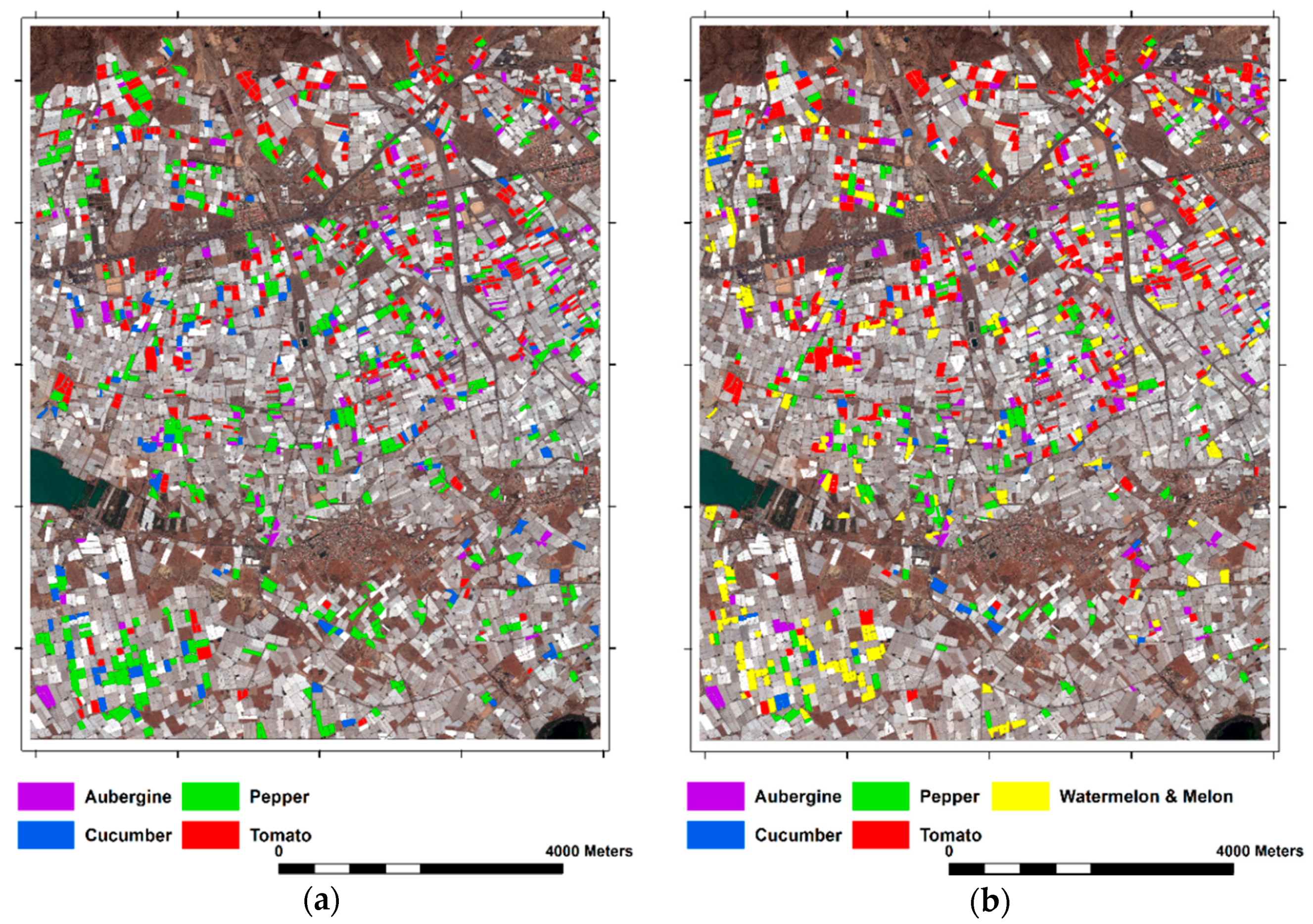
One of them was conducted in autumn 2016, from the end of October to the beginning of November. In this first fieldwork, 1202 individual PCG evenly distributed over the study area were inventoried. More specifically, 511, 379, 148, and 164 individual PCG containing pepper, tomato, aubergine, and cucumber, respectively, were monitored during the autumn field campaign (Figure 2a). The second fieldwork was undertaken at the end of April 2017 (spring campaign). In this case, 1114 individual greenhouses (225 pepper, 394 tomato, 161 aubergine, 64 cucumber, and 270 melon or watermelon) were visited (Figure 2b). It should be noted that the field campaigns were extremely time-consuming; the monitored greenhouses, both in autumn 2016 and spring 2017, were very representative of the main horticultural crops of the study area and the entire province of Almería. In fact, 849 greenhouses were visited in both field campaigns, while the rest were selected to maintain an adequate proportion of the different horticultural crops. The average area of the reference greenhouses took a value of 7279 m2, showing a very high standard deviation (4002 m2).
The typical dates of transplantation (T) and removal (R) of the main horticultural crops under plastic in the province of Almería turn out to be very variable according to the crop variety, crop cycle (long or short crop cycle), and the market conditions (Table 3).

4. Methodology

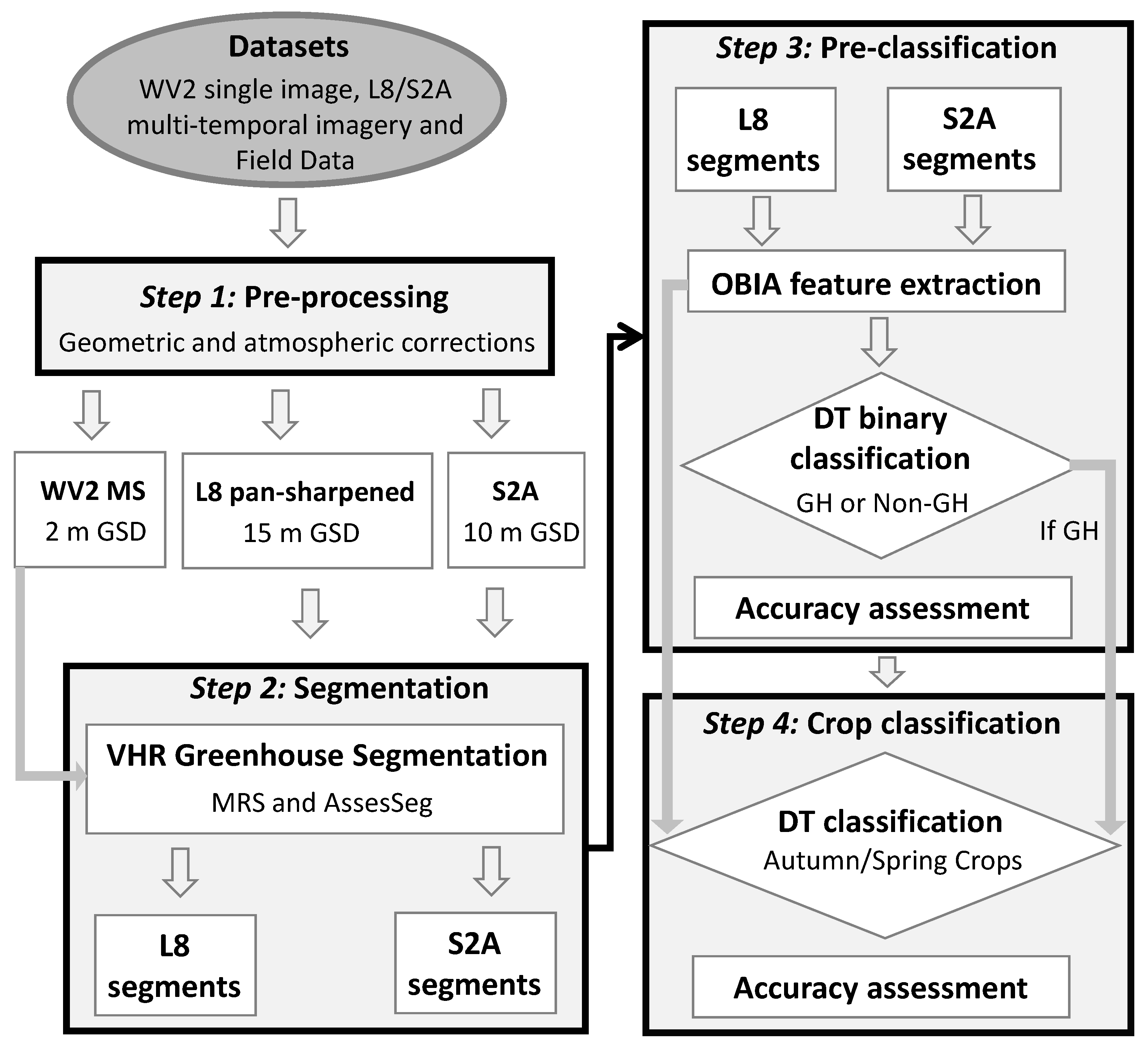
The methodology proposed in this article addresses the following aspects: (i) pre-processing protocol for WV2, L8, and S2A images (explained in Section 3.1, Section 3.2 and Section 3.3); (ii) segmentation of the WV2 MS orthoimage for delineating greenhouses; (iii) binary pre-classification of the entire study area into two classes (GH and Non-GH) by applying an OBIA approach based on the WV2 MS orthoimage segmentation and data from the L8 and S2A image time series; (iv) final classification of the main horticultural crops under PCG (Table 3) in autumn 2016 and spring 2017. A flowchart describing the methodology proposed is shown in Figure 3.

4.1. Segmentation

The original approach relied on employing the WV2 MS geometrically and atmospherically corrected imagery from 2015 to obtain a good segmentation over the study area. In fact, Aguilar et al. [30] reported that the VHR satellite atmospherically corrected MS orthoimage was the best satellite imagery source to attain a good segmentation dealing with PCG. Moreover, the segmentation process using an orthoimage with improved geometric resolution (e.g., PAN or pan-sharpened) required an extremely high computing time in our study area.
The widely known multi-resolution (MRS) image segmentation algorithm implemented in the OBIA software eCognition Version 8.8 was used in this work. This segmentation approach is a bottom–up region-merging technique that starts with one-pixel objects. In several iterative steps, smaller objects are merged into larger ones [31]. This task highly depends on the target objects to be segmented [32]. The MRS algorithm is controlled by three main factors: (i) the scale parameter (SP), which determines the maximum heterogeneity allowed for the resulting segments; (ii) the weight of color and shape criteria in the segmentation process (Shape); and (iii) the weight of the compactness and smoothness criteria (Compactness). Users must also configure the combination of bands combination and their corresponding weights to be applied in the segmentation process. More information about its mathematical formulation can be found in Baatz and Schäpe [31], Tian and Chen [32] and in the eCognition reference book [33].
Novelli et al. [17,34] obtained the optimal parameter for the MRS algorithm in the case of the WV2 MS orthoimage that was employed in this work. The selection of the best MRS parameters was undertaken through a modified version of the supervised discrepancy measure Euclidean Distance 2 (ED2) that was originally proposed by Liu et al. [35]. It is included in a free access command line tool named AssesSeg [34,36]. It is worth noting that 400 reference PCG objects, which were manually delineated on the WV2 orthoimage, were taken as reference objects [17] to compute the modified ED2. The aforementioned works showed that this number of reference objects is sufficient to guarantee a very good segmentation result at the considered study site.
The best segmentation attained for the WV2 MS orthoimage from the results achieved in Novelli et al. [17,34] was transferred to the L8 and S2A time series using the chessboard segmentation algorithm implemented in eCognition. For instance, the segmentation from WV2 MS 2015 was uploaded into the eCognition project as a vector thematic layer, and then projected onto the 14 L8 image time series. It is important to highlight that:
  • The 15-m GSD of the L8 pan-sharpened orthoimages was increased to 0.937 m by halving four times the original pixel size. This was necessary to guaranty a better fit between the L8 segmentations (the entire L8 time series) and the WV2 segmentation. A more in-depth explanation of this process is provided in Aguilar et al. [11].
  • In the case of S2A images (the entire S2A time series), the 10-m GSD was also increased to 1.25 m by halving three times the original pixel size, following the same methodology that was used for L8 pan-sharpened orthoimages.
  • In other words, L8 and S2A segmentations were derived from the best WV2-based segmentation in order to improve the final results by taking advantage of the better spatial resolution of the WV2 data.

4.2. Definition and Extration of Object-Based Features

The object-based features that were used in this work to accomplish the two-step OBIA classification (binary pre-classification in GH and Non-GH classes, plus the final crop labeling) were retrieved from the L8 (eight bands) and S2A (10 bands) image time series. The mean and standard deviation (SD) values of the BOA reflectance values for all the pixels within an object for each band and type of orthoimage (L8 pan-sharpened and S2A time series) were labeled as basic spectral information. The rest of the features consisted of several spectral and vegetation indices for both L8 (20 indices) and S2A (35 indices) single images. Note that one specific object (a greenhouse, for instance) will have 14 single values for each object-feature in the case of L8 time series data, but also for S2A. Table 4 shows the object features tested in this study for L8 (16 basic spectral information features and 20 indices). For the calculation of the Moment Distance Index (MDI), the Moment Distance from the Left pivot, and the Moment Distance from the Right pivot [12,19], λ represents the wavelength expressed in μm, ρ represents the normalized reflectance values ranging from 0 to 1, the subscript LP denotes the left pivot (located in a shorter wavelength), and the subscript RP denotes the right pivot (located in a longer wavelength).
In the case of the S2A images, Table 5 depicts the 20 basic spectral information features (mean and SD of the 10 bands) and 16 specific indices that were only tested for S2A. It should be noted that all of the indices shown in Table 4 for L8 images, with the exception of Cirrus NIR (i.e., 19 indices), were also tested for S2A images. The extraction of the single object-based features (Table 4 and Table 5) was carried out by transferring the WV2 MS orthoimage segmentation to the L8 and S2A image time series within the eCognition software environment (see Section 4.2).
The idea of introducing the features from WV2 MS orthoimage in the classification process was discarded in order to obtain classification results that were totally independent of the VHR data that was used to carry out the segmentation stage. In other words, the aim was to build a decision tree model only based on L8 or S2A features in order to avoid training in subsequent campaigns.
The texture features based on the gray-level co-occurrence matrix (GLCM) proposed by Haralick et al. [56] were not considered because they did not add any valuable information for PCG mapping or under PCG crops identification [11,12,17].
In addition, six statistical seasonal features were also computed from both the L8 and S2A image time series. Those features were the MAX (maximum), MIN (minimum), DIF (difference between MAX and MIN), MEAN (mean value), SD (Standard Deviation) and NOR, a seasonal feature defined as the normalized value of DIF ((MAX − MIN)/(MAX + MIN)). This approach was already used by Zillmann et al. [57] and Aguilar et al. [12] for grassland and PCG mapping, respectively. They reported that seasonal statistics should be more consistent than the snapshot values that were attained from the original single images.
The six statistical seasonal features were computed for all 14 images composing the L8 and S2A time series in the stage of GH and Non-GH binary pre-classification. Regarding the final crop classification stage, the image time series from L8 and S2A were split into two groups (see Section 3.4): (i) autumn crops included the first eight images (Table 1 and Table 2) taken from June to December 2016; and (ii) spring crops included three images taken from July to August 2016 and another six images acquired between February and June 2017. Regardless of the number of images considered in the L8 and S2A time series, the number of statistical seasonal features was always 216 and 330 for L8 (36 × 6) and S2A (55 × 6), respectively (see Table 4 and Table 5).

4.3. Decision Tree Modeling

A decision tree (DT) classifier based on the algorithm proposed by Breiman et al. [58] was used for the two different classification stages, i.e., binary pre-classification and final crop identification. DT is a non-parametric rule-based machine learning method in which each node makes a binary decision that separates either one class or some of the classes from the remaining class (or classes). The choice of this classifier resides both in its structure (formed by several splits) and in the easy interpretation of the final results (terminal leaves). Although other classifiers such as Random Forest or Support Vector Machine (black box classifiers) could achieve better classification results, DT provides clear decision rules with fixed threshold values that can be used in further works without any training phase. Furthermore, the classification through the DT algorithm has already been applied in greenhouse mapping from remote sensing data with very good and robust results [10,12]. DT has also been the selected classifier in OBIA investigations that have focused on both outdoor crops [22,23] and under PCG crops identification [11].
STATISTICA v10 was used for the classification and regression decision tree analysis (StatSoft Inc., Tulsa, OK, USA). The algorithm implemented in STATISTICA v10 is a classification trees algorithm that was designed to implement discriminant-based splits among the input predictors. From a computational point of view, it has been adapted from the QUEST (Quick, Unbiased, Efficient Statistical Trees) algorithm designed by Loh and Shih [59]. Lastly, the DT algorithm seeks to split the data into segments as homogeneously as possible with respect to the dependent or response variable. The DT node-splitting rule was the Gini index, which is a measure of impurity for a given node [60].

4.4. Accuracy Assessment for Binary Pre-Classification

The binary pre-classification assigned a class (GH or Non-GH) to each previously segmented object in the study area using the object-based features extracted from L8 and S2A image time series. A dataset composed of 1500 segments for the GH class and 1500 for the Non-GH class (i.e., non-crop reference plots), which were well distributed in the study area, was selected from the WV2 MS segmentation by means of a visual-based sampling procedure. For the selection of this dataset, several orthoimages from WV2, L8, and S2A were consulted to assure that all these 3000 objects represented meaningful objects for each class in 2016 and 2017, so as to avoid mixed segments. The 1500 selected Non-GH objects corresponded to bare soil, building, vegetation, and roads.
The categorical dependent variable for the DT model was the class (GH or Non-GH), while the statistical seasonal features were selected as the continuous predictor variables. This binary pre-classification analysis was performed for L8 and S2A image time series.
Cross-validation was used in this work for attaining an objective measure of quality for the computed DT model [11,23,61]. The experimental design was implemented within the STATISTICA environment through a stratified 10-fold cross-validation procedure where all of the data are randomly partitioned into 10 equally sized samples. A single sample is used to validate the model, while the remaining nine samples are used to train the model. The cross-validation process is then repeated 10 times; thus, each one of the 10 samples is used exactly once as validation data. A final confusion matrix was obtained by summing all of them.
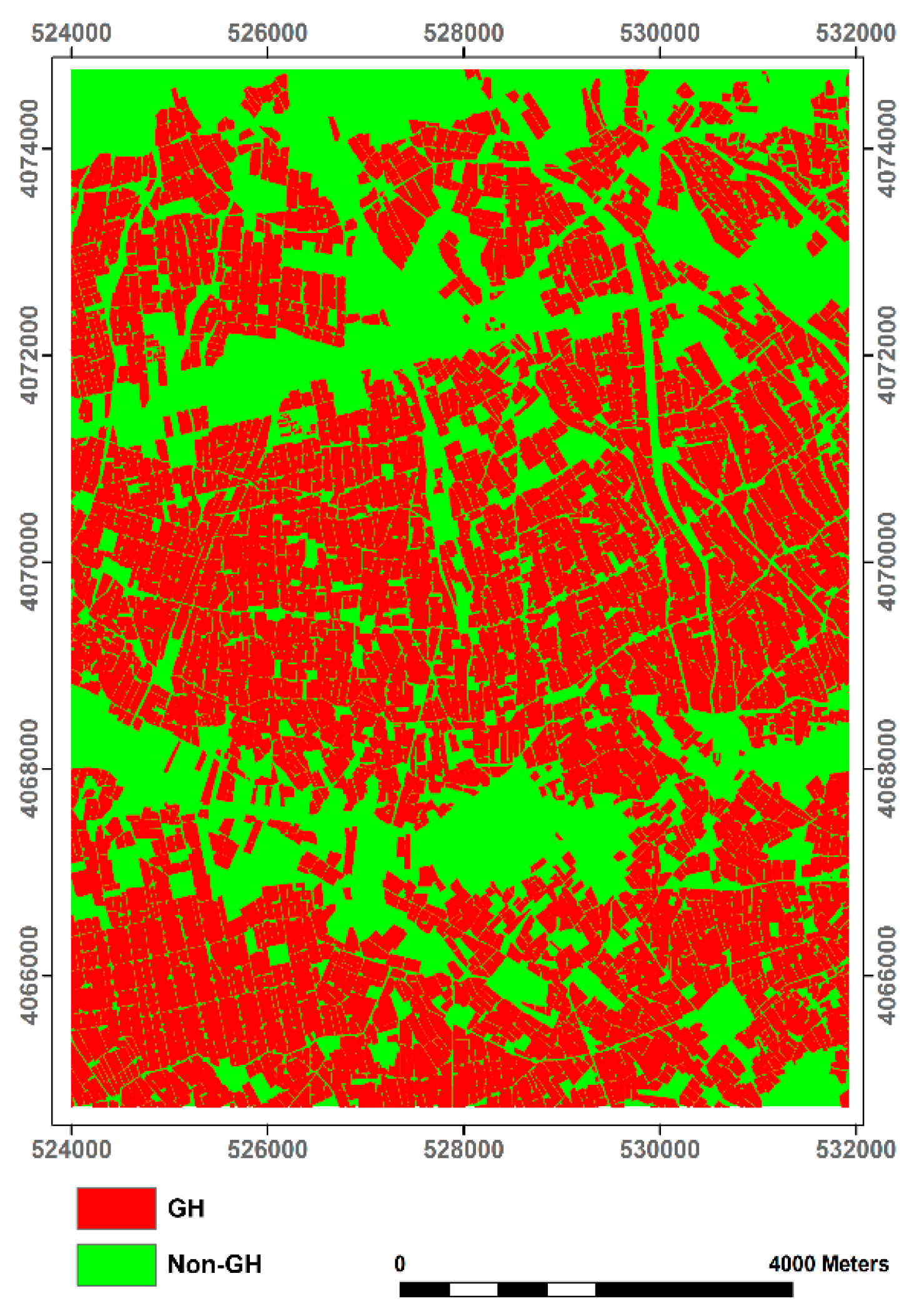
In the case of binary pre-classification, since this confusion matrix was based on meaningful objects, the errors related to the segmentation process and/or mixed objects were not considered. In addition, and according to Aguilar et al. [12], a more realistic classification accuracy assessment based on a real ground truth comprising the entire study area was carried out. This real ground truth, in vector format, was manually digitized over the WV2 pan-sharpened orthoimage to visually classify the final delineated polygons in GH or Non-GH. For this task, the L8 and S2A image time series were also used to update the ground truth, which was finally exported as a raster file with 2-m pixel size. The classification accuracy assessment for the binary pre-classification stage was based on the ground truth shown in Figure 4 and a pixel-based error matrix. In this way, the error coming from the previous segmentation phase over the entire study area, instead of a sample of it, was taken into account. The accuracy measures computed were overall accuracy (OA) and kappa coefficient (kappa) [62].

4.5. Accuracy Assessment for Crops Classification

Once the binary pre-classification has been completed, the objects assigned to the GH class were re-classified according to the under PCG crop in both autumn 2016 and spring 2017. For this task, the reference crops (Figure 2) were used as ground truth. DT classifier and cross-validation were also applied in this stage, but now selecting the type of crop under PCG as the categorical dependent variable. Note that we counted on 1202 reference greenhouses during autumn 2016 and 1114 during spring 2017. Both in the autumn and spring campaigns, cucumber and aubergine crops were grouped into one class named “Others”, because they showed an extreme variability in their spectral signature. Furthermore, both the statistical seasonal features and single features from L8 and S2A images were tested as the continuous predictor variables. The accuracy measures computed for the crops classification phase were user’s accuracy (UA), producer’s accuracy (PA), OA, and kappa [62], but in this case, and according to Aguilar et al. [11], the resulting confusion matrices were only based on objects instead of pixels. Finally, the Fβ measure [63], which provides a way of combining UA and PA into a single measure, was also computed according to Equation (1), where the parameter β determines the weight given to the accuracy computed as PA or UA. The value used in this study (β = 1) weighs UA equal to PA.
F β = ( β 2 + 1 ) × PA × UA β 2 × PA + UA
An internal buffer of 5 m or 10 m inside the segmented greenhouse polygons was applied to avoid the likely mixed pixels located at the borders, which is a very usual issue related to the use of medium-resolution satellite imagery. The size of the internal buffer was automatically selected, depending on the value of an object-based geometry feature included in eCognition named “Width [for 2D Image Objects]”. The Width feature is calculated from the WV2 MS segmentation by dividing the total number of pixels contained in a polygon (representing a greenhouse in this case) by the length/width ratio of this object [33]. When the Width value was less than or equal to 35, then the internal buffer that was applied was 5 m. Otherwise, it took a value of 10 m.

5. Results and Discussion

5.1. Segmentation

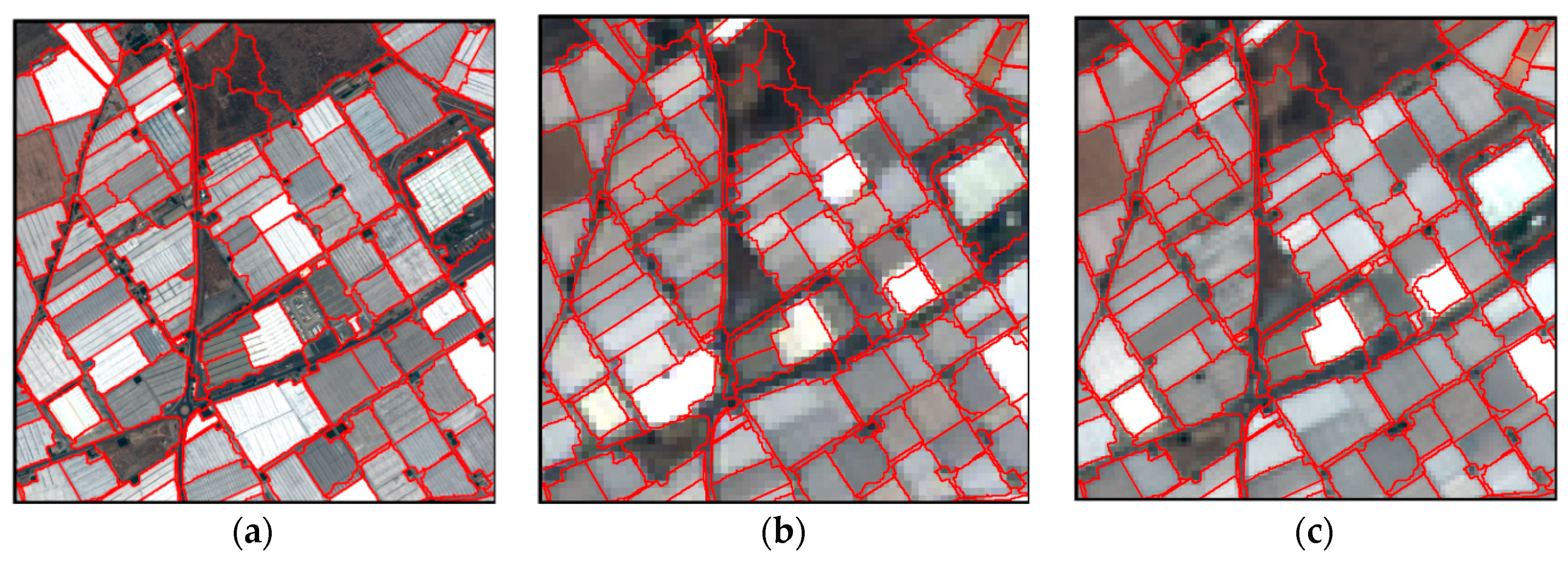
The optimal setting parameters reported by Novelli et al. [17] for the MRS algorithm applied to the WV2 MS atmospherically corrected orthoimage taken in July 2015 were used in this work. Therefore, the band combination was set to Blue–Green–NIR2 equally weighted. The SP, Shape, and Compactness parameters set to perform the MRS segmentation were 37.0, 0.4, and 0.5, respectively, yielding a modified ED2 value of 0.198 and a segmentation composed of 10,990 objects for the entire study area. Note that the best segmentation reported by Aguilar et al. [12] for the same WV2 MS orthoimage, but using all eight equally weighted bands and the original ED2 metric proposed by Liu et al. [35], was reached with values of 34.0, 0.3, and 0.5 for SP, Shape, and Compactness, respectively. In this case, the attained ED2 value of 0.290 was clearly worse than the one achieved here by using the AssesSeg command tool and the Modified ED2 metric. Figure 5 shows, in a detailed view, the segmentations attained for WV2 MS ATCOR orthoimage (Figure 5a), L8 pan-sharpened images (Figure 5b), and S2A scenes (Figure 5c).
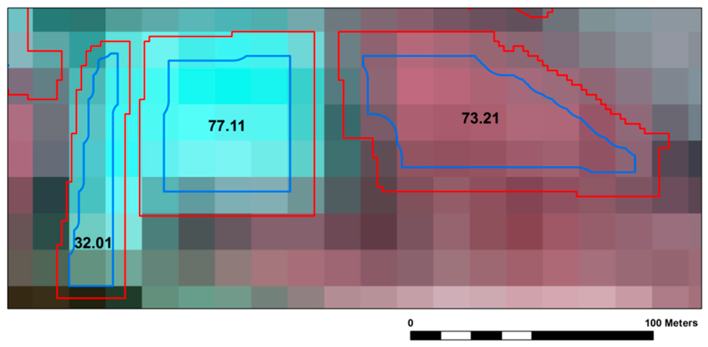
Figure 6 displays an example of the internal buffer application for the reference greenhouses depending on the value of the Width (the number located at the center of each greenhouse). Values of Width are less than or equal to 35 indicated greenhouses of small size and elongated shape. In this case, an internal buffer of 5 m was applied (e.g., object on the left in Figure 6). In greenhouses with Width values higher than 35, an internal buffer of 10 m was applied. For instance, looking at the greenhouse on the right in Figure 6, the mixed pixels that were situated close to the borders were avoided by using the proposed internal buffer.

5.2. Binary Pre-Classification

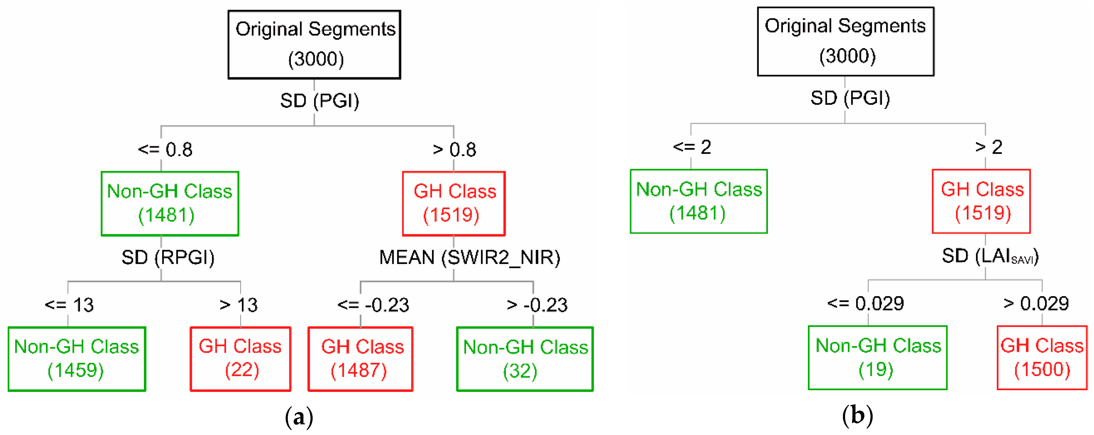
Figure 7 shows the DT models computed from the L8 (Figure 7a) and S2A (Figure 7b) image time series based on the 3000 reference objects manually classified as GH or Non-GH. The standard deviation of the Plastic Greenhouse Index (SD (PGI)) turned out to be the most significant statistical seasonal feature (first split in the DT model) for both time series, although the split threshold was different for L8 (0.8) and S2A (2.0). This was not surprising after having contrasted the radiometric differences between L8 and S2A in Section 5.1. In the case of L8 (Figure 7a), the other statistical seasonal features computed by the DT model to improve the final binary classification (secondary splits) were the standard deviation of the Retrogressive Plastic Greenhouse Index (SD (RPGI)) and the mean value of the normalized index for the SWIR2 and NIR bands (MEAN (SWIR2_NIR). In the case of S2A, the standard deviation of the Leaf Area Index–Soil Adjusted Vegetation Index values (SD (LAISAVI)) was the feature selected by the DT model to refine the binary classification (Figure 7b). The PGI proposed by Yang et al. [13] is an index that is very related to the vegetation beneath plastic cover, being higher when the crops inside the greenhouse are flourishing. Regarding our time series, the higher values of PGI were mainly obtained in November and December, which was just when the main crops were showing their maximum NDVI values. However, the values of PGI were very low (even negatives) in summer, coinciding with the greenhouses being whitewashed. That is, plastic sheets are usually painted white during summer to protect plants from excessive radiation and reduce the heat inside the greenhouse [64]. The good performance of SD (PGI) feature was actually based on this high range of variability over time to discriminate between GH and Non-GH classes. Yang et al. [13] also proposed the RPGI, a modified index of the PGI in which the term (NIR-R) was removed from the numerator of the PGI formula (Table 4). This index was also very variable for the GH class, although it was less sensitive to the crop under PCG. SWIR2_NIR [12] presented very high negative values for L8 images in greenhouses with flourishing crops. A behavior similar to that which was observed for the SWIR2_NIR index was found for LAISAVI [47] in S2A images, but always presenting positive values.
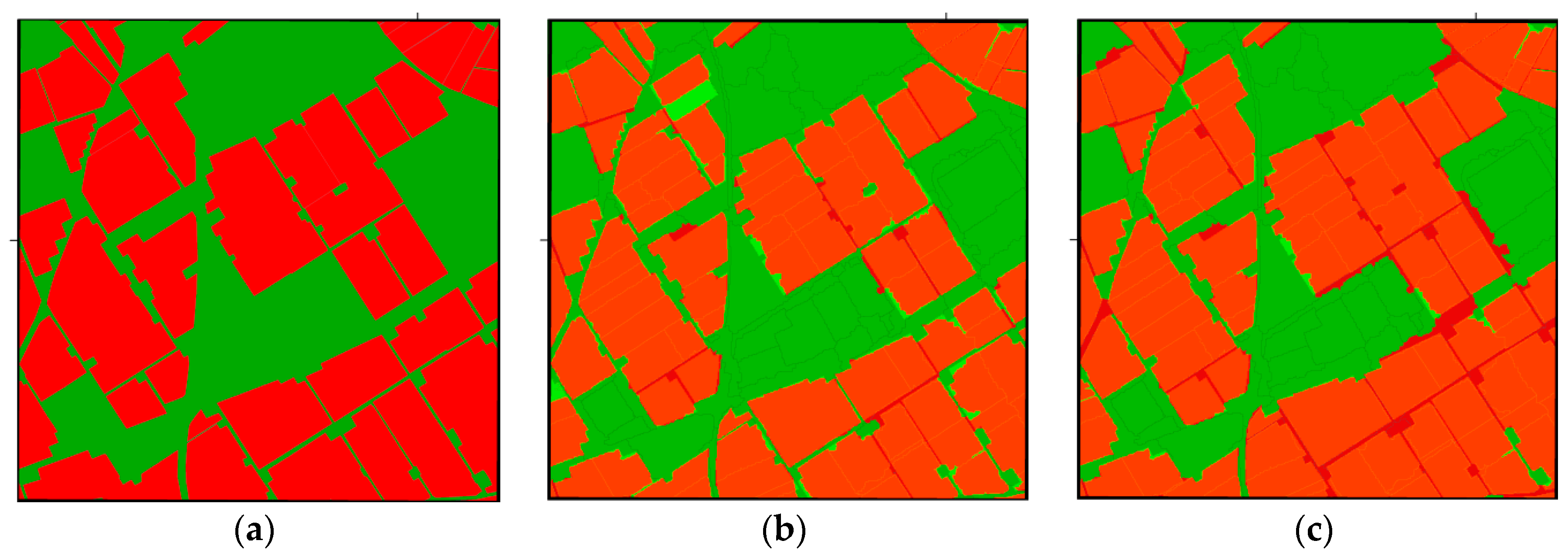
Regarding the OA and kappa values obtained from the pixel-based accuracy assessment for the entire study area, the results from S2A DT (OA = 93.97%; Kappa = 0.875) were slightly better than those attained from L8 DT (OA = 92.65%; Kappa = 0.846). Note that the segmentation quality is also included in these pre-classification accuracy assessment results. Figure 8 displays the binary pre-classification from applying the proposed DT models for both L8 and S2A image time series in a square area with 1000-m sides (previously used in Figure 5). Comparing the L8 classification map (Figure 8c) with the ground truth depicted in Figure 8a, we can see that the main source of error in brown was located at the elongated objects situated between greenhouses, where Non-GH objects (narrow streets) were classified as GH due to the presence of mixed pixels [4,12]. These misclassification errors were greatly reduced in the case of the S2A classification map (Figure 8b) due to its higher spatial resolution. The second, and smaller source of error, was related to the classification obtained from the proposed DT models. Very good OA values of 99.80% and 99.37% were achieved for L8 and S2A respectively when carrying out a cross-validation accuracy assessment based on the selected 3000 meaningful objects (GH and Non-GH). In this way, there was only one greenhouse incorrectly classified as Non-GH for S2A in Figure 8b. This greenhouse presented a value for SD (PGI) of 1.98, which turned out to be slightly lower than the threshold in Figure 8b. In the case of L8, this same greenhouse had values for SD (PGI) and SD (RPGI) of 0.73 and 20.18 respectively, which was correctly classified as GH thanks to SD (RPGI) split. This type of misclassification error (objects wrongly classified as Non-GH) was usually related to the decrease in the typical variability of reflectance values in cultivated greenhouses (e.g., newly constructed or renovated greenhouses without crop during the field campaign). This is also the case of greenhouses covered by using double-screen films with an air chamber created between the two films (anti-drip effect in cucumber). The opposite case (i.e., objects wrongly classified as GH) was related to new buildings (industrial or farm buildings) built throughout the completion of the study.
In order to test whether the threshold values depicted in Figure 7 were sufficiently robust, two new classification maps were generated for L8 and S2A, but now using two time series composed of seven images covering the studied campaign (i.e., choosing the odd or even images corresponding to their chronological order in Table 1 and Table 2). The OA values obtained for the two sets of seven images were quite similar to the ones obtained in the case of 14 images for both L8 and S2A (L8 Set 1: OA = 92.78%; L8 Set 2: OA = 91.79%; S2A Set 1: OA = 93.62%; S2A Set 2: OA = 93.74%). These accuracy values were much more stable over the time than those reported by Lu et al. [10,65] working with time series from Landsat 5 TM and MODIS.
Aguilar et al. [12] reported OA of 92.3% and 92.42% for two time series (years 2014 and 2015) of pan-sharpened L8 images in the same study area. In that work, a DT model based only on the minimum value of the Moment Distance Index (MIN (MDI)) and the difference between maximum and minimum values of SWIR1 (DIF (SWIR1)) was built for the two L8 time series. An OA of 90.56% was attained when this DT model was applied to our L8 data (14 images). This value can be considered quite good, considering that the used cutting thresholds were the same computed by Aguilar et al. [12]. Anyway, the PGI proposed by Yang et al. [13] proved to be the most significant object-based feature to perform an accurate binary pre-classification regarding GH and Non-GH classes for the two medium spatial resolution sensors that were tested. Moreover, its use in the form of a statistical seasonal feature resulted in very accurate and temporally stable classification results.

5.3. Crop Classification

After the data pre-processing, segmentation, and binary pre-classification stages, the next step deals with the automatic identification of crops under PCG over two seasons: autumn 2016 and spring 2017.
Table 6 depicts the results obtained from the accuracy assessment carried out for crop classification using DT models restricted to seven to eight terminal nodes. Different strategies were considered for the two agronomic seasons using single object-based features or statistical seasonal features extracted from L8 or S2A image time series (i.e., L8 single, S2A single, L8 seasonal, S2A seasonal). In autumn 2016, the OA values ranged from 72.96 to 75.87%. Aguilar et al. [11] achieved very similar results (OA = 75.90%) in the identification of autumn crops under PCG in the same study area. They also used seven to eight terminal nodes DT models and single features extracted from L8 multi-temporal images. In this case, OA values of up to 81.3% were attained from using a DT model of 34 terminal nodes [12]. The main problem of this very complex DT model with a high number of terminal nodes seems to be their reproducibility in the years thereafter. In this sense, in this work, simpler DT models were trained and validated to extract knowledge from the statistical seasonal features in order to compute more consistent DT threshold values over years, making the multi-temporal approach less dependent on the availability of particular acquisition dates and less sensitive to missing data on crucial dates.
Table 6 shows that the classification accuracies attained from single or statistical seasonal features for both L8 and S2A were similar (Table 6). In spring 2017, the OA values were very close to those attained in autumn 2016, although a new class was included in this season (melon or watermelon (Melon&W)).
The type of sensor (L8 and S2A) did not clearly influence the final crop classification accuracy, although S2A single always yielded slightly better results. The OA values attained in this work for both seasons, ranging from 72.44% to 75.87%, are rather promising as compared to those reported by other authors who worked with a similar methodology but over outdoor crops. In this way, a very similar OA (76%) was achieved by Immitzer et al. [66] using an object-based approach for mapping crop types using a single S2A image and a supervised Random Forest classifier (RF). Peña-Barragán et al. [23] reached an OA of 79% from applying a DT classifier to detecting 13 major outdoor crops using multi-temporal ASTER satellite scenes. Inglada et al. [67] reported an OA above 80% for most sites around the world using RF. In another study, 12 outdoor crops and two non-vegetative land-use classes were classified with 80.7% OA at the cadastral parcel level through multi-temporal remote sensing images [68]. Using DT and 13 Landsat 8 multi-temporal images, Patil et al. [69] achieved an OA of 81%, while an OA of 88% was reported by Zhong et al. [70] working on corn, soybean, and others, and using Landsat imagery. An OA of 94% was reported by Vieira et al. [23] by applying the DT classifier to Landsat time series in a binary classification approach to label sugarcane and other crops. Finally, Belgiu and Csillik [71] achieved better results in cropland mapping from Sentinel-2 time series using an object-based instead of a pixel-based approach, reporting overall accuracies ranging from 78.05% to 96.19%.
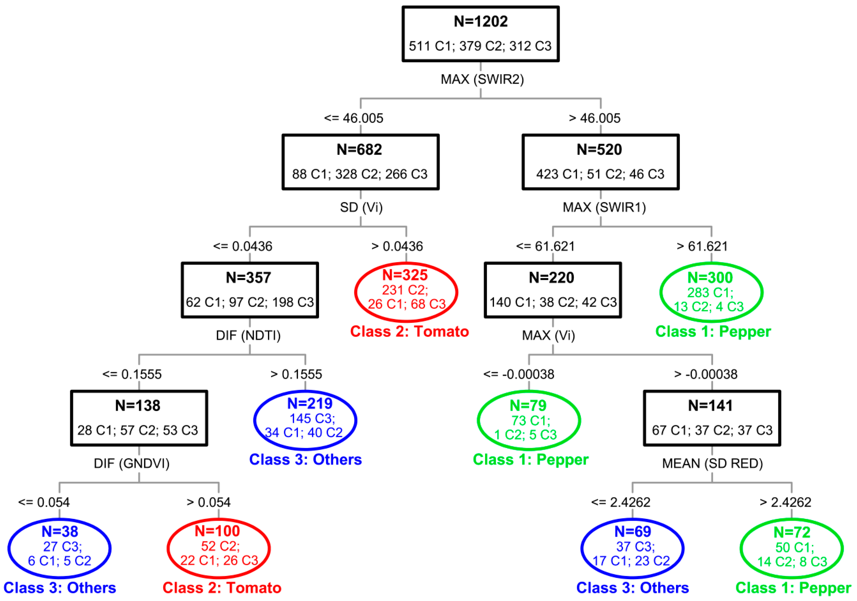
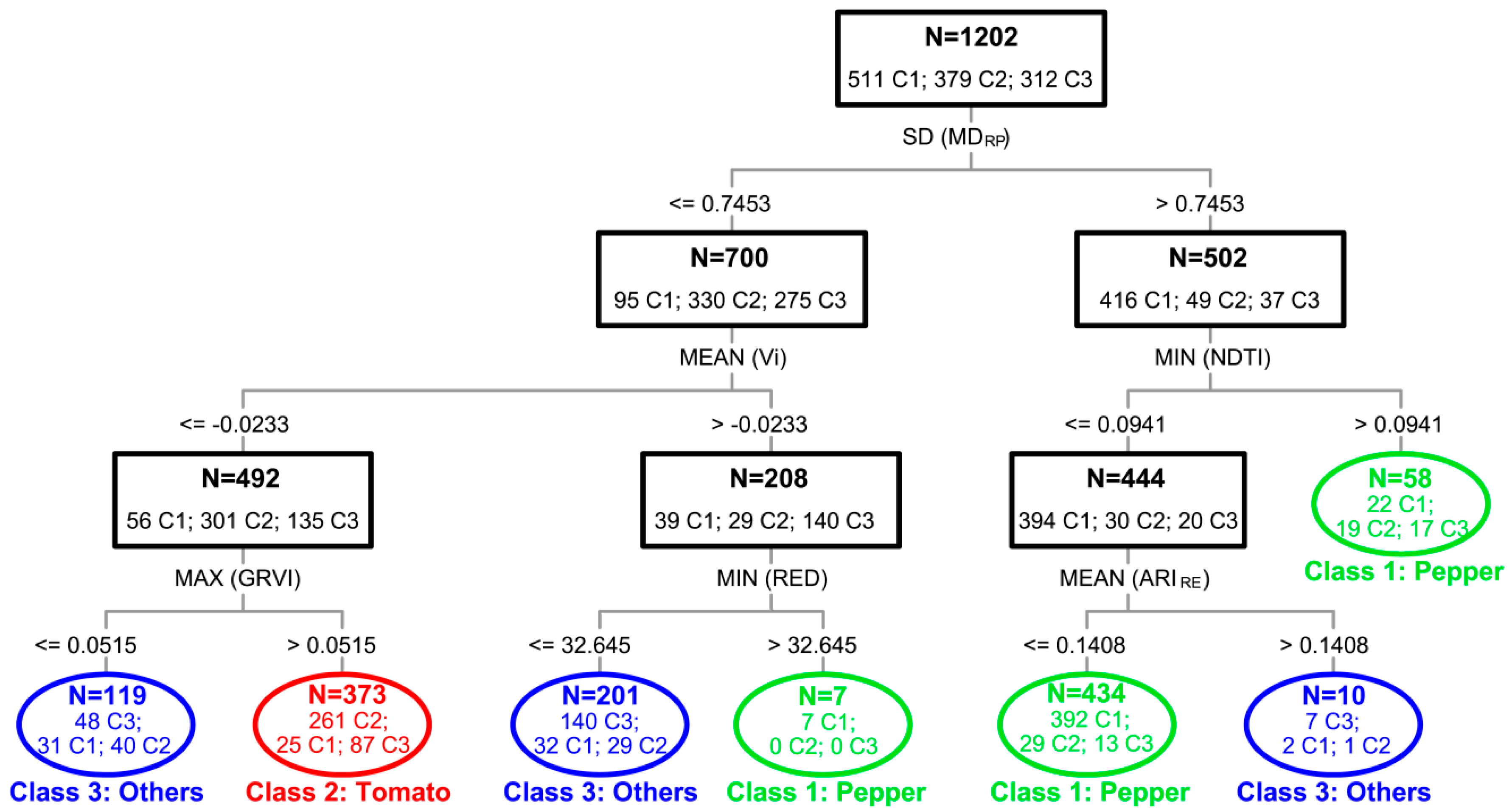
Table 6 also shows the accuracy per class in terms of Fβ. In autumn 2016, pepper was the most accurately classified crop, yielding an Fβ of around 84%, followed by tomato (Fβ values close to 70%) and others (including cucumber and aubergine) with Fβ values of around 62%. Also dealing with autumn crops, Aguilar et al. [11] reported Fβ values of around 87% for pepper, but worse in cucumber and aubergine crops, with Fβ values ranging from 50% to 63%. According to Aguilar et al. [11], the most defining characteristic for pepper identification turned out to be the unique whitewashing management in the case of this crop, which is mainly planted during July and August, needing a significant quantity of whitewash in summer to both enhance the growth of the plant and protect the transplant stage against heat. Therefore, the high reflectance values for SWIR1 and SWIR2 bands in the months of July and August were related to the high level of white paint applied to the greenhouses containing pepper. In this way, the L8 autumn DT is depicted in Figure 9. At the bottom and outside of each black box in Figure 9 appears the statistical seasonal feature that is causing the next split in the DT. Below, readers can see the figure corresponding to the cutting threshold for each split. Oval nodes are terminal nodes belonging to a certain class. Inside each black box or terminal node (oval), there is information about the number of total objects (N) and the distribution by classes of those objects. In this sense, the maximum value of SWIR2 was the first split for the L8 autumn DT. The MAX (SWIR2) cutting threshold (46.005) provided the first pepper and non-pepper (tomato and others) split. In fact, only 69 out of the 520 greenhouses with MAX (SWIR2) values higher than 46.005 were finally classified as non-pepper. In the case of S2A (Figure 10), the first split was computed from the standard deviation of the Moment Distance from the Right pivot (SD (MDRP)). The MDRP is defined as the sum of the hypotenuses constructed from the right pivot located at the maximum wavelength band (i.e., SWIR2 for S2A) to the value at successively shorter wavelengths [72]. Its SD values resulted in extremely high when the greenhouse had been strongly painted in summer; so, pointing to the pepper class. It is important to underline that similar and quite good OA values of 84.61% and 84.94% for L8 and S2A, respectively, were yielded from using only the first splits mentioned above in a binary classification exercise (pepper and non-pepper classes). For the rest of the autumn crops (cucumber, aubergine, and tomato), there was no such clear rule to classify them, although good performance in distinguishing tomato crops was attained through applying statistical seasonal features based on single features such as Index Greenhouse Vegetable Land Extraction (Vi) [18], vegetation indices (NDTI, GNDVI, and GRVI, defined in Table 4), and mean spectral values per object (SD RED).
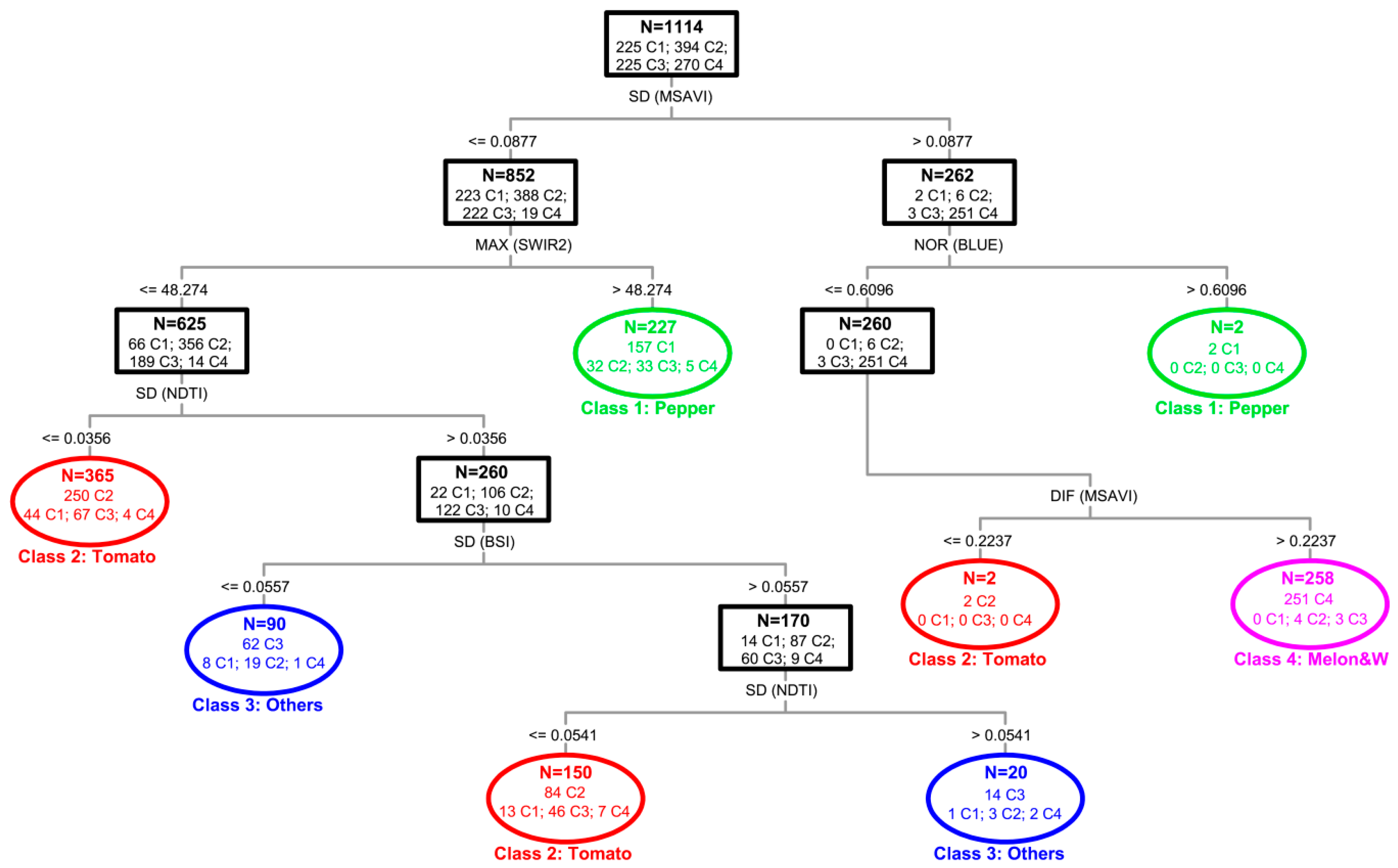
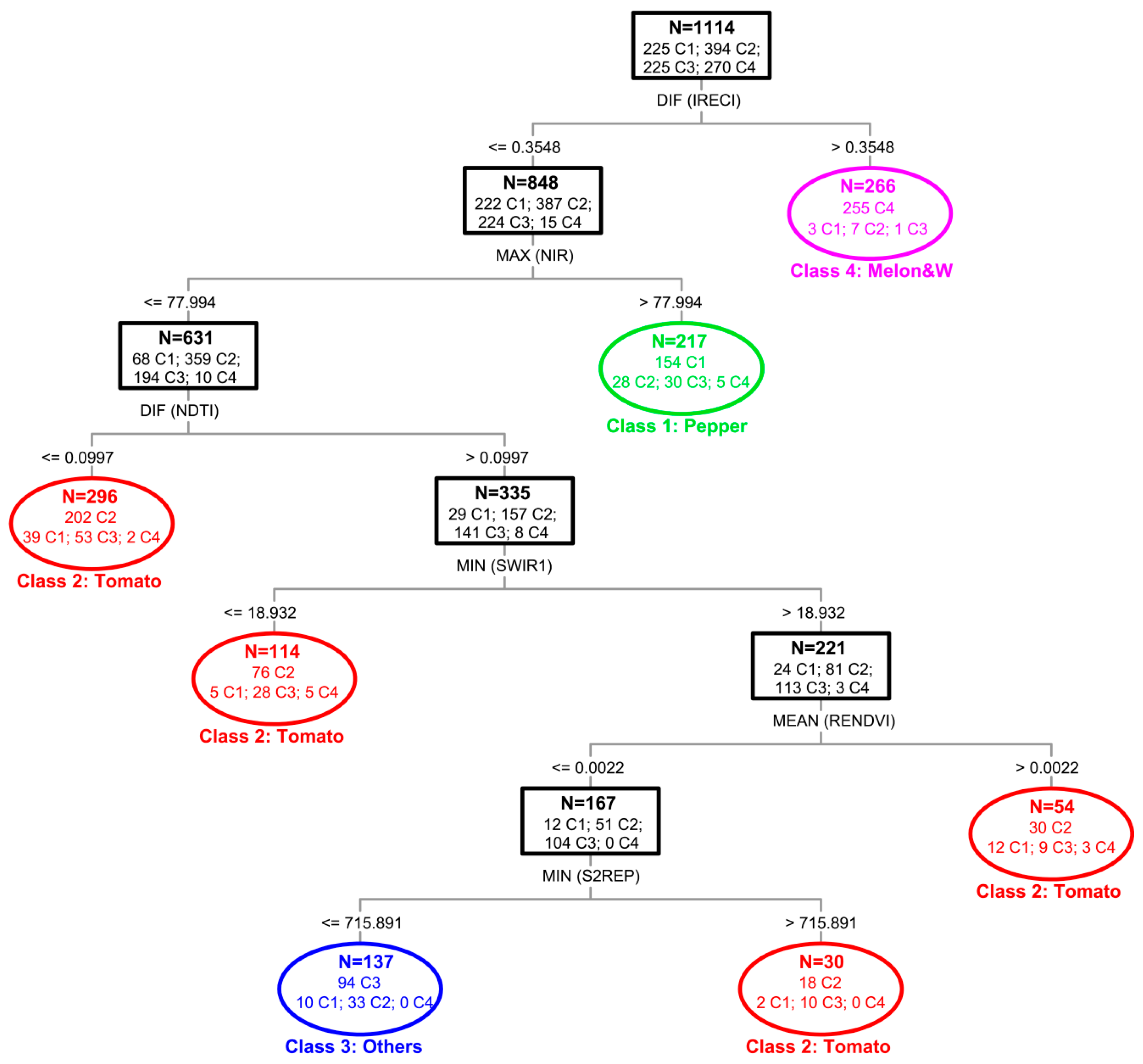
In spring 2017, the Melon&W class was the best classified, with impressive Fβ values of around 94.6% (Table 6). Note that the melon and watermelon crops cultivated under greenhouse in Almería require full sun for proper growth, so the plastic sheet is usually maintained totally clean. This makes these horticultural crops easily detectable in the months of April or May, when they are in their maximum production stage, since they present high photosynthetic activity as compared to other contemporary crops. Figure 11 displays the L8 DT for the spring season, being the Standard Deviation of the Modified Soil-Adjusted Vegetation Index [42] (SD (MSAVI)) the feature located at the first split. Greenhouses with values of SD (MSAVI) in spring higher than 0.0877 were basically identified as Melon&W (258 out of 262). In the left branch, pepper crops were again discriminated from tomato and others thanks to MAX (SWIR2) statistical feature, which was directly related to the greenhouse being whitewashed in summer. Note that the set of nine images for both L8 and S2A that were used for the spring season included the three scenes taken in July and August. In the case of S2A (Figure 12), the first split was given by the difference of the Red-Edge Chlorophyll Index [51] (DIF (IRECI)). As for the L8 spring DT, the Class 4 (Melon&W) showed the highest DIF (IRECI) values. It is important to highlight that the OA values of 97.31% and 97.67% for L8 and S2A, respectively, were obtained from using very simple DT models, only including the first splits mentioned above in a binary classification exercise (Melon&W and Non-Melon&W classes). Tomato classification yielded slightly better accuracy figures in spring season than in autumn, while pepper and others attained worse results.

6. Conclusions

A workflow to carry out the identification of under PCG crops is proposed in this work through using an OBIA approach from multi-temporal (L8 and S2A time series) multi-sensor (WV2, L8, and S2A) satellite imagery. This workflow is composed of four stages: (i) Data pre-processing, (ii) Segmentation, (iii) Binary pre-classification in GH or Non-GH, and (iv) Classification of under greenhouse crops in two agronomic seasons: autumn 2016 and spring 2017.
Regarding the segmentation stage, the automatic greenhouses delineation was ideally achieved using the widely known MRS algorithm applied to the WV2 MS atmospherically corrected orthoimage. The use of the free access command tool named AssesSeg allowed to set the optimal parameters for the MRS algorithm. This segmentation based on a VHR satellite image was then transferred to the L8 and S2A image time-series project. It is worth mentioning that the AssesSeg tool can work with segmentation algorithms other than MRS. Therefore, the evaluation of segmentation does not strictly depend on the use of eCognition.
The next step consisted of the binary pre-classification of the previously segmented objects in GH or Non-GH. The DT classifier was applied to determine the best statistical seasonal features (MEAN, MAX, MIN, DIF, SD, and NOR defined as DIF ((MAX − MIN)/(MAX + MIN))) derived from several groups of single object-based features (spectral, vegetation indices, and plastic detection indices). The single object-based features were extracted from each L8 and S2A single pre-processed scene. Two very simple DT models were developed for L8 and S2A. The standard deviation of the Plastic Greenhouse Index (SD (PGI)) was the most important statistical seasonal feature for both image time series, although the cutting threshold value took different values for L8 and S2A. The OA and kappa accuracy values for the binary classification achieved from S2A DT (OA = 93.97%; Kappa = 0.875) were slightly better than the ones attained from L8 DT (OA = 92.65%; Kappa = 0.846), showing that the misclassification errors, mainly in the elongated objects representing streets between greenhouses, were greatly reduced in the case of S2A classification map thanks to its higher spatial resolution (10-m GSD for S2A and 15-m GSD for L8 pan-sharpened). According to our best knowledge, this is the first work in which several indices for PCG detection have been compared in the same conditions for L8 and S2A images, concluding that the PGI index reported by Yang et al. [14] proved to be the most outstanding. Furthermore, it was shown that a very accurate and stable classification of individual greenhouses can be achieved by only using the proposed DT models, meaning that the results are highly transferable because the classifier training phase would not be required.
The last step addressed the classification of crops under PCG. The classification accuracies attained from single or statistical seasonal features for both L8 and S2A were similar. Since the main objective of this study was to obtain robust and consistent DT models, making the multi-temporal approach less dependent on the availability of particular acquisition dates and less sensitive to missing data on crucial dates, we focused on working with the more stable statistical seasonal features. Note that implementing an internal buffer for extracting object features in the crop classification phase may have diminished the possible differences between L8 and S2A due to ground pixel size. In autumn 2016, OA values of 74.04% and 72.96% were achieved for L8 and S2A seasonal features, respectively. In that season, pepper was the best-classified crop, presenting Fβ values of around 84% while tomato reached Fβ values of around 70%. Finally, the class Others (cucumber and aubergine) yielded clearly poorer results. In spring 2017, similar OA values to those observed in autumn were attained for L8 (73.79%) and S2A (74.42%). In this season, the Melon&W class achieved impressive accuracies (Fβ) better than 95% for L8 and S2A, while tomato (73.5%), pepper (70%), and others (48%) presented significantly worse results. Actually, pepper, in autumn, and Melon&W, in spring, were the only two crops classified with great consistency. The good results that were found for pepper classification were due to the high reflectance values in the SWIR1 and SWIR2 bands, which was an effect related to the practice of applying a significant quantity of white paint in summer (July and August) to protect crops against heat. In fact, MAX (SWIR2) and SD (MDRP) were the most important statistical seasonal features for pepper detection using L8 and S2A, respectively. In the case of Melon&W, the high levels of photosynthetic activity in April or May, together with the high transparency of the plastic sheets, made this crop easily detectable, in which SD (MSAVI) for L8 and DIF (IRECI) for S2A were the most significant features.
Overall, the proposed workflow has been successfully proved from using WV2, L8, and S2A satellite images, showing that S2A time series yielded slightly better accuracies than L8, mainly in the binary pre-classification phase. However, further works are needed to learn much more about the influence on the classification of crops under PCG of several factors such as crops varieties, type, age, and thickness of the plastic cover, and greenhouse roof geometry.

Author Contributions

A.N. (Abderrahim Nemmaoui) collected the input data and performed the experiments, additionally collaborating in manuscript writing and revision M.A.A. proposed the methodology, designed and conducted the experiments, and contributed extensively in manuscript writing and revision. F.J.A. made significant contributions to the research design and manuscript preparation, providing suggestions for the methodology design and conducting the data analysis and manuscript revision. A.N. (Antonio Novelli) carried out the segmentation tests and collected the object-based features. A.G.L. was the people in charge of facilitate the fieldwork and contacting the agricultural cooperatives in the area.

Funding

This research was funded by the Spanish Ministry of Economy and Competitiveness (Spain) and the European Union (European Regional Development Fund, ERDF), grant number AGL2014-56017-R.

Acknowledgments

This work was supported by the Spanish Ministry of Economy and Competitiveness (Spain) and the European Union (European Regional Development Fund, ERDF) funds (Grant Reference AGL2014-56017-R). It takes part of the general research lines promoted by the Agrifood Campus of International Excellence ceiA3 (http://www.ceia3.es/). We are grateful to José Manuel Fernández and Manuel Galdeano from Vicasol and Murgiverde Agricultural Cooperatives for their crucial cooperation in this work.

Conflicts of Interest

The authors declare no conflict of interest.

References

  1. Foley, J.A.; Ramankutty, N.; Brauman, K.A.; Cassidy, E.S.; Gerber, J.S.; Johnston, M.; Mueller, N.D.; O’Connell, C.; Ray, D.K.; West, P.C.; et al. Solutions for a Cultivated Planet. Nature 2011, 478, 337–342. [Google Scholar] [CrossRef] [PubMed]
  2. Espi, E.; Salmerón, A.; Fontecha, A.; García, Y.; Real, A.I. Plastic films for agricultural applications. J. Plast. Film Sheet. 2006, 22, 85–102. [Google Scholar] [CrossRef]
  3. Briassoulis, D.; Dougka, G.; Dimakogianni, D.; Vayas, I. Analysis of the collapse of a greenhouse with vaulted roof. Biosyst. Eng. 2016, 151, 495–509. [Google Scholar] [CrossRef]
  4. Wu, C.F.; Deng, J.S.; Wang, K.; Ma, L.G.; Tahmassebi, A.R.S. Object-based classification approach for greenhouse mapping using Landsat-8 imagery. Int. J. Agric. Biol. Eng. 2016, 9, 79–88. [Google Scholar] [CrossRef]
  5. Matton, N.; Canto, G.S.; Waldner, F.; Valero, S.; Morin, D.; Inglada, J.; Arias, M.; Bontemps, S.; Koetz, B.; Defourny, P. An automated method for annual cropland mapping along the season for various globally-distributed agrosystems using high spatial and temporal resolution time series. Remote Sens. 2015, 7, 13208–13232. [Google Scholar] [CrossRef]
  6. Atzberger, C. Advances in remote sensing of agriculture: Context description, existing operational monitoring systems and major information needs. Remote Sens. 2013, 5, 949–981. [Google Scholar] [CrossRef]
  7. Song, X.-P.; Potapov, P.V.; Krylov, A.; King, L.; Di Bella, C.M.; Hudson, A.; Khan, A.; Adusei, B.; Stehman, S.V.; Hansen, M.C. National-scale soybean mapping and area estimation in the United States using medium resolution satellite imagery and field survey. Remote Sens. Environ. 2017, 190, 383–395. [Google Scholar] [CrossRef]
  8. Wulder, M.A.; Coops, N.C.; Roy, D.P.; White, J.C.; Hermosilla, T. Land cover 2.0. Int. J. Remote Sens. 2018, 39, 4254–4284. [Google Scholar] [CrossRef] [Green Version]
  9. Li, J.; Roy, D.P. A Global Analysis of Sentinel-2A, Sentinel-2B and Landsat-8 Data Revisit Intervals and Implications for Terrestrial Monitoring. Remote Sens. 2017, 9, 902. [Google Scholar] [CrossRef]
  10. Lu, L.; Di, L.; Ye, Y. A Decision-Tree classifier for extracting transparent Plastic-Mulched landcover from landsat-5 TM images. IEEE J. Sel. Top. Appl. Earth Observ. Remote Sens. 2014, 7, 4548–4558. [Google Scholar] [CrossRef]
  11. Aguilar, M.A.; Vallario, A.; Aguilar, F.J.; García Lorca, A.; Parente, C. Object-Based Greenhouse Horticultural Crop Identification from Multi-Temporal Satellite Imagery: A Case Study in Almeria, Spain. Remote Sens. 2015, 7, 7378–7401. [Google Scholar] [CrossRef] [Green Version]
  12. Aguilar, M.A.; Nemmaoui, A.; Novelli, A.; Aguilar, F.J.; García Lorca, A. Object-Based Greenhouse Mapping Using Very High Resolution Satellite Data and Landsat 8 Time Series. Remote Sens. 2016, 8, 513. [Google Scholar] [CrossRef]
  13. Yang, D.; Chen, J.; Zhou, Y.; Chen, X.; Chen, X.; Cao, X. Mapping plastic greenhouse with medium spatial resolution satellite data: Development of a new spectral index. ISPRS J. Photogramm. Remote Sens. 2017, 128, 47–60. [Google Scholar] [CrossRef]
  14. Hasituya; Chen, Z. Mapping Plastic-Mulched Farmland with Multi-Temporal Landsat-8 Data. Remote Sens. 2017, 9, 557. [Google Scholar] [CrossRef]
  15. Lanorte, A.; De Santis, F.; Nolè, G.; Blanco, I.; Loisi, R.V.; Schettini, E.; Vox, G. Agricultural plastic waste spatial estimation by Landsat 8 satellite images. Comput. Electron. Agric. 2017, 141, 35–45. [Google Scholar] [CrossRef]
  16. González-Yebra, Ó.; Aguilar, M.A.; Nemmaoui, A.; Aguilar, F.J. Methodological proposal to assess plastic greenhouses land cover change from the combination of archival aerial orthoimages and Landsat data. Biosyst. Eng. 2018, 175, 36–51. [Google Scholar] [CrossRef]
  17. Novelli, A.; Aguilar, M.A.; Nemmaoui, A.; Aguilar, F.J.; Tarantino, E. Performance evaluation of object based greenhouse detection fromSentinel-2 MSI and Landsat 8 OLI data: A case study from Almería (Spain). Int. J. Appl. Earth Obs. Geoinf. 2016, 52, 403–411. [Google Scholar] [CrossRef]
  18. Zhao, G.; Li, J.; Li, T.; Yue, Y.; Warner, T. Utilizing landsat TM imagery to map greenhouses in Qingzhou, Shandong Province, China. Pedosphere 2004, 14, 363–369. [Google Scholar]
  19. Salas, E.A.L.; Henebry, G.M. Separability of maize and soybean in the spectral regions of chlorophyll and carotenoids using the Moment Distance Index. Isr. J. Plant Sci. 2012, 60, 65–76. [Google Scholar] [CrossRef]
  20. Badhwar, G. Classification of Corn and Soybeans Using Multitemporal Thematic Mapper Data. Remote Sens. Environ. 1984, 16, 175–181. [Google Scholar] [CrossRef]
  21. Petitjean, F.; Kurtz, C.; Passat, N.; Gançarski, P. Spatio-temporal reasoning for the classification of satellite image time series. Pattern Recognit. Lett. 2012, 33, 1805–1815. [Google Scholar] [CrossRef] [Green Version]
  22. Peña-Barragán, J.M.; Ngugi, M.K.; Plant, R.E.; Six, J. Object-based crop identification using multiple vegetation indices, textural features and crop phenology. Remote Sens. Environ. 2011, 115, 1301–1316. [Google Scholar] [CrossRef] [Green Version]
  23. Vieira, M.A.; Formaggio, A.R.; Rennó, C.D.; Atzberger, C.; Aguiar, D.A.; Mello, M.P. Object based image analysis and data mining applied to a remotely sensed Landsat time-series to map sugarcane over large areas. Remote Sens. Environ. 2012, 123, 553–562. [Google Scholar] [CrossRef]
  24. Berk, A.; Bernstein, L.S.; Anderson, G.P.; Acharya, P.K.; Robertson, D.C.; Chetwynd, J.H.; Adler-Golden, S.M. MODTRAN Cloud and Multiple Scattering Upgrades with Application to AVIRIS. Remote Sens. Environ. 1998, 65, 367–375. [Google Scholar] [CrossRef]
  25. United States Geological Survey (USGS). EarthExplorer Download Tool. Available online: https://earthexplorer.usgs.gov/ (accessed on 27 June 2018).
  26. Levin, N.; Lugassi, R.; Ramon, U.; Braun, O.; Ben-Dor, E. Remote sensing as a tool for monitoring plasticulture in agricultural landscapes. Int. J. Remote Sens. 2007, 28, 183–202. [Google Scholar] [CrossRef]
  27. European Space Agency (ESA). Copernicus Open Access Hub. Available online: https://scihub.copernicus. eu/dhus/#/home (accessed on 27 June 2018).
  28. Main-Knorn, M.; Pflug, B.; Debaecker, V.; Louis, J. Calibration and validation plan for the L2A processor and products of the Sentinel-2 mission. Int. Arch. Photogramm. Remote Sens. Spat. Inf. Sci. 2015, XL-7/W3, 1249–1255. [Google Scholar] [CrossRef] [Green Version]
  29. Müller-Wilm, U. Sentinel-2 MSI-Level-2A Prototype Processor Installation and User Manual. Available online: http://step.esa.int/thirdparties/sen2cor/2.2.1/S2PAD-VEGA-SUM-0001-2.2.pdf (accessed on 27 June 2018).
  30. Aguilar, M.A.; Novelli, A.; Nemmaoui, A.; Aguilar, F.J.; García Lorca, A.M.; González-Yebra, O. Optimizing Multiresolution Segmentation for Extracting Plastic Greenhouses from WorldView-3 Imagery. In Intelligent Interactive Multimedia Systems and Services 2017; KES-IIMSS-18 2018, Smart Innovation, Systems and Technologies; De Pietro, G., Gallo, L., Howlett, R., Jain, L., Eds.; Springer: Cham, Switzerland, 2018; Volume 76. [Google Scholar] [CrossRef]
  31. Baatz, M.; Schäpe, M. Multiresolution Segmentation—An Optimization Approach for High Quality Multi-Scale Image Segmentation. In Angewandte Geographische Informations-Verarbeitung XII; Strobl, J., Blaschke, T., Griesebner, G., Eds.; Wichmann Verlag: Karlsruhe, Germany, 2000; pp. 12–23. [Google Scholar]
  32. Tian, J.; Chen, D.M. Optimization in multi-scale segmentation of high resolution satellite images for artificial feature recognition. Int. J. Remote Sens. 2007, 28, 4625–4644. [Google Scholar] [CrossRef]
  33. Trimble Germany GmbH. eCognition Developer 8.8 Reference Book; Trimble Germany GmbH: Munich, Germany, 2012. [Google Scholar]
  34. Novelli, A.; Aguilar, M.A.; Aguilar, F.J.; Nemmaoui, A.; Tarantino, E. AssesSeg—A command line tool to quantify image segmentation quality: A test carried out in Southern Spain from satellite imagery. Remote Sens. 2017, 9, 40. [Google Scholar] [CrossRef]
  35. Liu, Y.; Biana, L.; Menga, Y.; Wanga, H.; Zhanga, S.; Yanga, Y.; Shaoa, X.; Wang, B. Discrepancy measures for selecting optimal combination of parameter values in object-based image analysis. ISPRS-J. Photogramm. Remote Sens. 2012, 68, 144–156. [Google Scholar] [CrossRef]
  36. Novelli, A.; Aguilar, M.A.; Aguilar, F.J.; Nemmaoui, A.; Tarantino, E. C_AssesSeg Concurrent Computing Version of AssesSeg: A Benchmark Between the New and Previous Version. In Computational Science and Its Applications—ICCSA 2017; Lecture Notes in Computer Science; Springer: Cham, Switzerland, 2017; Volume 10407, pp. 45–56. [Google Scholar] [CrossRef]
  37. Merzlyak, M.N.; Gitelson, A.A.; Chivkunova, O.B.; Solovchenko, A.E.; Pogosyan, S.L. Application of reflectance spectroscopy for analysis of higher plant pigments. Russ. J. Plant Physiol. 2003, 50, 704–710. [Google Scholar] [CrossRef]
  38. Roy, P.S.; Sharma, K.P.; Jain, A. Stratification of density in dry deciduous forest using satellite remote sensing digital data—An approach based on spectral indices. J. Biosci. 1996, 21, 723–734. [Google Scholar] [CrossRef]
  39. Gitelson, A.A.; Kaufman, Y.J.; Merzlyak, M.N. Use of a green channel in remote sensing of global vegetation from EOS-MODIS. Remote Sens. Environ. 1996, 58, 289–298. [Google Scholar] [CrossRef]
  40. Gitelson, A.A.; Kaufman, Y.J.; Stark, R.; Rundquist, D. Novel algorithms for remote estimation of vegetation fraction. Remote Sens. Environ. 2002, 80, 76–87. [Google Scholar] [CrossRef] [Green Version]
  41. Qi, J.; Chehbouni, A.; Huete, A.R.; Kerr, Y.H.; Sorooshian, S. A modified soil adjusted vegetation index. Remote Sens. Environ. 1994, 48, 119–126. [Google Scholar] [CrossRef]
  42. Chen, J.M. Evaluation of vegetation indices and a modified simple ratio for boreal applications. Can. J. Remote Sens. 1996, 22, 229–242. [Google Scholar] [CrossRef]
  43. Zha, Y.; Gao, J.; Ni, S. Use of normalized difference built-up index in automatically mapping urban areas from TM imagery. Int. J. Remote Sens. 2003, 24, 583–594. [Google Scholar] [CrossRef]
  44. Rouse, J.W.; Haas, R.H.; Schell, J.A.; Deering, D.W. Monitoring Vegetation Systems in the Great Plains with ERTS. In Proceedings of the 1973 Earth Resources Technology Satellite-1 Symposium, Washington, DC, USA, 10–14 December 1973. [Google Scholar]
  45. Van Deventer, A.; Ward, A.; Gowda, P.; Lyon, J. Using thematic mapper data to identify contrasting soil plains and tillage practices. Photogramm. Eng. Remote Sens. 1997, 63, 87–93. [Google Scholar]
  46. Gitelson, A.A.; Merzlyak, M.N.; Zur, Y.; Stark, R.; Gritz, U. Non-Destructive and Remote Sensing Techniques for estimation of vegetation status. In Proceedings of the 3rd European Conference on Precision Agriculture, Montpelier, France, 18–20 June 2001; pp. 205–210. [Google Scholar]
  47. Sentinel Hub. Sentinel 2 EO Products. Available online: https://www.sentinel-hub.com/develop/documentation/eo_products/Sentinel2EOproducts (accessed on 10 July 2018).
  48. Waser, L.T.; Küchler, M.; Jütte, K.; Stampfer, T. Evaluating the potential of WorldView-2 data to classify tree species and different levels of ash mortality. Remote Sens. 2014, 6, 4515–4545. [Google Scholar] [CrossRef]
  49. Gitelson, A.A.; Keydan, G.P.; Merzlyak, M.N. Three-band model for noninvasive estimation of chlorophyll, carotenoids, and anthocyanin contents in higher plant leaves. Geophys. Res. Lett. 2006, 33, L11402. [Google Scholar] [CrossRef]
  50. Dash, J.; Curran, P.J. The MERIS terrestrial chlorophyll index. Int. J. Remote Sens. 2004, 25, 5403–5413. [Google Scholar] [CrossRef]
  51. Gao, B. NDWI -A Normalized Difference Water Index for Remote Sensing of Vegetation Liquid Water from Space. Remote Sens. Environ. 1996, 58, 257–266. [Google Scholar] [CrossRef]
  52. Frampton, W.J.; Dash, J.; Watmough, G.; Milton, E.J. Evaluating the capabilities of Sentinel-2 for quantitative estimation of biophysical variables in vegetation. ISPRS J. Photogramm. Remote Sens. 2013, 82, 83–92. [Google Scholar] [CrossRef]
  53. Abdel-rahman, E.M.; Landmann, T.; Kyalo, R.; Ong, G.; Mwalusepo, S.; Sulieman, S.; Le, B. Predicting stem borer density in maize using RapidEye data and generalized linear models. Int. J. Appl. Earth Obs. Geoinf. 2017, 57, 61–74. [Google Scholar] [CrossRef]
  54. Jasper, J.; Reusch, S.; Link, A. Active sensing of the N status of wheat using optimized wavelength combination: Impact of seed rate, variety and growth stage. In Proceedings of the Precision Agriculture Conference, Wageningen, The Netherlands, 6–8 July 2009; Henten, E.J., van Goense, D., Lokhorst, C., Eds.; Wageningen Academic Publishers: Wageningen, The Netherlands, 2009; pp. 23–30. [Google Scholar]
  55. Chen, J.C.; Yang, C.M.; Wu, S.T.; Chung, Y.L.; Charles, A.L.; Chen, C.T. Leaf chlorophyll content and surface spectral reflectance of tree species along a terrain gradient in Taiwan’s Kenting National Park. Bot. Stud. 2007, 48, 71–77. [Google Scholar]
  56. Haralick, R.M.; Shanmugam, K.; Dinstein, I.H. Textural Features for Image Classification. IEEE Trans. Syst. Man Cybern. 1973, 3, 610–621. [Google Scholar] [CrossRef] [Green Version]
  57. Zillmann, E.; Gonzalez, A.; Montero Herrero, E.J.; van Wolvelaer, J.; Esch, T.; Keil, M.; Weichelt, H.; Garzón, A.M. Pan-European grassland mapping using seasonal statistics from multisensor image time series. IEEE J. Sel. Top. Appl. Earth Obs. Remote Sens. 2014, 7, 3461–3472. [Google Scholar] [CrossRef]
  58. Breiman, L.; Friedman, J.H.; Olshen, R.A.; Stone, C.I. Classification and Regression Trees; Chapman & Hall/CRC Press: Boca Raton, NY, USA, 1984. [Google Scholar]
  59. Loh, W.Y.; Shin, Y.-S. Split selection methods for classification trees. Stat. Sin. 1997, 7, 815–840. [Google Scholar]
  60. Zambon, M.; Lawrence, R.; Bunn, A.; Powell, S. Effect of alternative splitting rules on image processing using classification tree analysis. Photogramm. Eng. Remote Sens. 2006, 72, 25–30. [Google Scholar] [CrossRef]
  61. Peña-Barragán, J.M.; Gutiérrez, P.A.; Hervás-Martínez, C.; Six, J.; Plant, R.E.; López-Granados, F. Object-based image classification of summer crops with machine learning methods. Remote Sens. 2014, 6, 5019–5041. [Google Scholar] [CrossRef]
  62. Congalton, R.G. A review of assessing the accuracy of classifications of remotely sensed data. Remote Sens. Environ. 1991, 37, 35–46. [Google Scholar] [CrossRef]
  63. Aksoy, S.; Akcay, H.G.; Wassenaar, T. Automatic mapping of linear woody vegetation features in agricultural landscapes using very high-resolution imagery. IEEE Trans. Geosci. Remote Sens. 2010, 48, 511–522. [Google Scholar] [CrossRef] [Green Version]
  64. Aguilar, M.A.; Bianconi, F.; Aguilar, F.J.; Fernández, I. Object-based greenhouse classification from GeoEye-1 and WorldView-2 stereo imagery. Remote Sens. 2014, 6, 3554–3582. [Google Scholar] [CrossRef]
  65. Lu, L.; Hang, D.; Di, L. Threshold model for detecting transparent plastic-mulched landcover using moderate-resolution imaging spectroradiometer time series data: A case study in southern Xinjiang, China. J. Appl. Remote Sens. 2015, 9. [Google Scholar] [CrossRef]
  66. Immitzer, M.; Vuolo, F.; Atzberger, C. First Experience with Sentinel-2 Data for Crop and Tree Species Classifications in Central Europe. Remote Sens. 2016, 8, 166. [Google Scholar] [CrossRef]
  67. Inglada, J.; Arias, M.; Tardy, B.; Hagolle, O.; Valero, S.; Morin, D.; Dedieu, G.; Sepulcre, G.; Bontemps, S.; Defourny, P.; et al. Assessment of an Operational System for Crop Type Map Production Using High Temporal and Spatial Resolution Satellite Optical Imagery. Remote Sens. 2015, 7, 12356–12379. [Google Scholar] [CrossRef] [Green Version]
  68. García-Torres, L.; Caballero-Novella, J.J.; Gómez-Candón, D.; Peña-Barragén, J.M. Census parcels cropping system classification from multitemporal remote imagery: A proposed universal methodology. PLoS ONE 2015, 10, e0117551. [Google Scholar] [CrossRef] [PubMed]
  69. Patil, V.C.; Al-Gaadi, K.A.; Madugundu, R.; Tola, E.; Zeyada, A.M.; Marey, S.; Biradar, C.M. CART and IDC—Based classification of irrigated agricultural fields using multi-source satellite data. Geocarto Int. 2018, 33, 70–88. [Google Scholar] [CrossRef]
  70. Zhong, L.; Gong, P.; Binging, G.S. Efficient corn and soybean mapping with temporal extendability: A multi-year experiment using Landsat imagery. Remote Sens. Environ. 2014, 140, 1–13. [Google Scholar] [CrossRef]
  71. Belgiu, M.; Csillik, O. Sentinel-2 cropland mapping using pixel-based and object-based timeweighted dynamic time warping analysis. Remote Sens. Environ. 2018, 204, 509–523. [Google Scholar] [CrossRef]
  72. Salas, E.A.L.; Boykin, K.G.; Valdez, R. Multispectral and texture feature application in image-object analysis of summer vegetation in Eastern Tajikistan Pamirs. Remote Sens. 2016, 8, 78. [Google Scholar] [CrossRef]
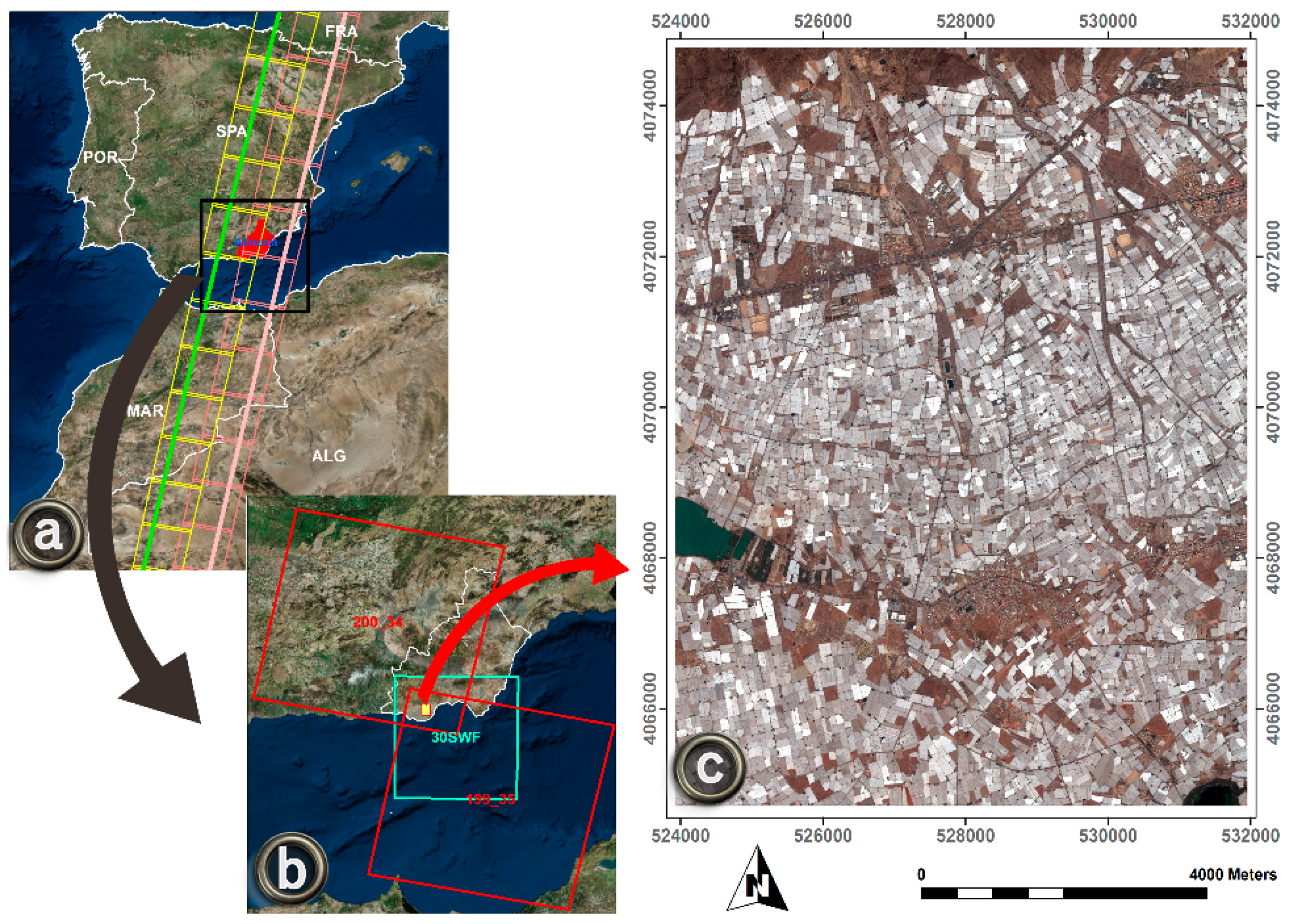
Figure 1. Location of the study area: (a) Province of Almeria localization (in red) showing the Landsat paths 200 and 199 (yellow and pink outlines respectively) and the Sentinel-2A relative orbits R094 and R051 (green and pink lines respectively); (b) Study area (yellow polygon) and the two scenes of Landsat 8 (200/34 and 199/35) and the scene of Sentinel-2A (30SWF) used in this study; (c) Detailed view of the study area based on a red–green–blue (RGB) WorldView-2 image taken in July 2015. Coordinate system: ETRS89 UTM Zone 30N.
Remotesensing 10 01751 g001
Figure 2. Location of the reference horticultural crops growing under plastic-covered greenhouses (PCG). Reference image: WorldView-2 (WV2) multispectral (MS) RGB orthoimage: (a) Field campaign carried out in autumn 2016; (b) Field campaign carried out in spring 2017.
Remotesensing 10 01751 g002
Figure 3. Flowchart of the methodology proposed in this work.
Remotesensing 10 01751 g003
Figure 4. Manually digitized ground truth (ETRS89 UTM coordinate system).
Remotesensing 10 01751 g004
Figure 5. Ideal segmentations achieved using the modified Euclidean Distance 2 (ED2) evaluation method on a detailed subarea (1000 m × 1000 m): (a) The best segmentation for WV2 MS image taken in July 2015; (b) The best segmentation transferred to L8 pan-sharpened images; and (c) The best segmentation transferred to S2A images.
Remotesensing 10 01751 g005
Figure 6. Application of an internal buffer of 5 m or 10 m to the segmented objects corresponding to the reference greenhouses depending on the value of Width (the number in the center of each greenhouse). The background image corresponds to the false color (near infrared, NIR; red, R; green, G) Landsat 8 scene taken in November 2016.
Remotesensing 10 01751 g006
Figure 7. Decision Tree (DT) models proposed for the binary pre-classification (greenhouse, GH and non-greenhouse, Non-GH) based on stable statistical seasonal features: (a) For the 14 images from Landsat 8 (L8), and (b) For the 14 images from S2A.
Remotesensing 10 01751 g007
Figure 8. Pixel-based accuracy assessment for the developed DT models over the same detailed area used in Figure 5 (1000 m × 1000 m): (a) Manually digitized ground truth; (b) Classification results using the DT model for S2A; and (c) Classification results using the DT model for L8. The GH class is represented in red, and the Non-GH class is represented in green. Light green and brown colors in both classification maps highlight the misclassification errors.
Remotesensing 10 01751 g008
Figure 9. Decision tree computed for the L8 dataset in autumn 2016 using statistical seasonal features (i.e., MEAN, MAX, MIN, DIF, SD, and NOR). N is the number of objects in each node, Class 1 (C1) = Pepper, C2 = Tomato, C3 = Others (i.e., Cucumber and Aubergine), NOR = DIF ((MAX − MIN)/(MAX + MIN)).
Remotesensing 10 01751 g009
Figure 10. Decision tree computed for the S2A dataset in autumn 2016 using statistical seasonal features (i.e., MEAN, MAX, MIN, DIF, SD, and NOR). N is the number of objects in each node, Class 1 (C1) = Pepper, C2 = Tomato, C3 = Others (i.e., Cucumber and Aubergine).
Remotesensing 10 01751 g010
Figure 11. Decision tree computed for the L8 dataset in spring 2017 using statistical seasonal features (i.e., MEAN, MAX, MIN, DIF, SD, and NOR). N is the number of objects in each node, Class 1 (C1) = Pepper, C2 = Tomato, C3 = Others (i.e., Cucumber and Aubergine), C4 = Melon&W (i.e., Melon and Watermelon).
Remotesensing 10 01751 g011
Figure 12. Decision tree computed for the S2A dataset in spring 2017 using statistical seasonal features (i.e., MEAN, MAX, MIN, DIF, SD, and NOR). N is the number of objects in each node, Class 1 (C1) = Pepper, C2 = Tomato, C3 = Others (i.e., Cucumber and Aubergine), C4 = Melon&W (i.e., Melon and Watermelon).
Remotesensing 10 01751 g012
Table 1. Characteristics of the Landsat 8 Operational Land Imager (OLI) images.
PathRowDate of Acquisition
(Day/Month/Year)
Start Time
(UTC)
Sun Azimuth
(Degrees)
Sun Elevation
(Degrees)
199359 June 201610:43:50120.2567.76
2003418 July 201610:50:09124.6464.65
1993512 August 201610:44:27131.4160.96
2003419 August 201610:50:17136.8658.58
1993513 September 201610:44:38146.0952.72
1993531 October 201610:44:45159.5037.21
200347 November 201610:50:31160.9233.88
2003425 December 201610:50:25158.9226.14
2003427 February 201710:50:03148.9839.21
2003415 March 201710:49:55146.5245.22
199359 April 201710:43:55140.1655.59
200342 May 201710:49:27135.8361.80
2003418 May 201710:49:39130.4765.19
1993512 June 201710:43:50119.6367.78
Table 2. Characteristics of the Sentinel-2A images.
OrbitGranuleDate of Acquisition
(Day/Month/Year)
Start Time
(UTC)
Sun Azimuth
(Degrees)
Sun Elevation
(Degrees)
R09430SWF13 June 201611:05:59132.4271.65
R09430SWF23 July 201611:07:12135.1168.14
R09430SWF12 August 201610:56:22142.9164.02
R05130SWF19 August 201610:50:32141.4761.07
R05130SWF18 September 201610:50:22153.9552.19
R09430SWF31 October 201611:02:02166.9838.16
R05130SWF7 November 201610:52:42164.5635.56
R05130SWF27 December 201610:54:42161.8327.93
R09430SWF28 February 201711:00:01155.7442.62
R09430SWF10 March 201710:58:41154.6346.45
R09430SWF9 April 201710:56:51150.9358.11
R05130SWF6 May 201710:50:31139.8165.44
R09430SWF19 May 201710:56:51140.5469.43
R05130SWF5 June 201710:50:31129.3469.89
Table 3. Schematic summary of the typical dates of transplantation (T) and removal (R) for the studied horticultural crops. From June (month number 6) to June.
CropMonth
6789101112123456
Tomato TT TT/RT/RTRRR
PepperTTTTT RRRRRRR
Aubergine TT R RRRRR
Cucumber TTTT/RRRT/RT/RRRRR
Melon or Watermelon TTTRRR
Table 4. Landsat 8 single images’ object-based features. The features with an asterisk (*) were also applied to Sentinel-2A images.
NameDefinitionsReferences
Mean and Standard Deviation (SD) (16 features)Mean and SD of each pan-sharpened L8 band[33]
BRI (Browning Reflectance Index) * ( ( 1 / G ) ( 1 / R ) ) / NIR [37]
BSI (Bare Soil Index) * ( ( SWIR 1 + R ) ( NIR + B ) ) / ( ( SWIR 1 + R ) + ( NIR + B ) ) [38]
Cirrus_NIR ( CI NIR ) / ( CI + NIR ) [12]
GNDVI (Green NDVI) * ( NIR G ) / ( NIR + G ) [39]
GRVI (Green Red Vegetation Index) * ( G R ) / ( G + R ) [40]
MDLP (Moment Distance from the Left pivot) * MD LP = i = λ LP λ RP ( ρ i 2 + ( i λ LP ) 2 ) [19]
MDRP (Moment Distance from the Right pivot) * MD RP = i = λ RP λ LP ( ρ i 2 + ( λ RP i ) 2 ) [19]
MDI (Moment Distance Index) * MD RP MD LP [19]
GDI (Greenhouse Detection Index) * ( MDI / 3 ) ( ( B ( SWIR 1 + SWIR 2 ) / 2 ) / ( B + ( SWIR 1 + SWIR 2 ) / 2 ) ) [16]
MSAVI (Modified Soil-Adjusted Vegetation Index) * ( 2 × NIR + 1 ( ( 2 × NIR + 1 ) 2 8 × ( NIR R ) ) / 2 [41]
MSR (Modified Simple Ratio) * ( ( NIR / R ) 1 ) / ( NIR / R + 1 ) [42]
NDBI (Normalized Difference Built-up Index) * ( SWIR 1 NIR ) / ( SWIR 1 + NIR ) [43]
NDVI (Normalized Difference Vegetation Index) * ( NIR R ) / ( NIR + R ) [44]
NDTI (Normalized Difference Tillage Index) * ( SWIR 1 SWIR 2 ) / ( SWIR 1 + SWIR 2 ) [45]
PGI (Plastic Greenhouse Index) * 100 × ( B × ( NIR R ) / ( 1 ( B + G + NIR ) / 3 ) [13]
PMLI (Plastic-Mulched Landcover Index) * ( SWIR 1 R ) / ( SWIR 1 + R ) [10]
RPGI (Retrogressive Plastic Greenhouse Index) * ( 100 × B ) / ( 1 ( B + G + NIR ) / 3 ) [13]
SW1_SW2_NIR * ( ( SWIR 1 + SWIR 2 ) / 2 NIR ) / ( ( SWIR 1 + SWIR 2 ) / 2 + NIR ) [12]
SWIR2_NIR * ( SWIR 2 NIR ) / ( SWIR 2 + NIR ) [12]
Vi (Index Greenhouse Vegetable Land Extraction) * ( ( SWIR 1 NIR ) / ( SWIR 1 + NIR ) ) × ( ( NIR R ) / ( NIR + R ) ) [18]
Table 5. Sentinel-2A single images’ object-based features.
NameDefinitionsReferences
Mean and Standard Deviation (SD) (20 features)Mean and SD of each S2A band[33]
ARI (Anthocyanin Reflectance Index) ( NIR / B ) ( NIR / G ) [46]
ARIRE (modified Anthocyanin Reflectance Index) ( 1 / G ) ( 1 / RE 1 ) [46,47]
BR (Blue Ratio) ( R / B ) × ( G / B ) × ( RE 1 / B ) × ( NIR / B ) [48]
CIRE (Chlorophyll Red-Edge Index) ( NIR / RE 1 ) 1 [49]
CRI2 (Carotenoid Reflectance Index 2) ( 1 / B ) ( 1 / RE 1 ) [46]
IRECI (Red-Edge Chlorophyll Index) ( RE 3 R ) / ( RE 1 / RE 2 ) [50]
LAISAVI (Leaf Area Index–Soil Adjusted Vegetation Index) log ( 0.371 + 1.5 × ( NIR R ) / ( NIR + R + 0.5 ) ) / 2.4 [46]
Modified Swir1_NIR ( SWIR 1 RE 1 ) / ( SWIR 1 + RE 1 ) [12]
MTCI (MERIS Terrestrial Chlorophyll Index) ( RE 2 RE 1 ) / ( RE 1 R ) [51]
NDWIRE (Red-Edge Normalized difference Water Index) ( NNir SWIR 1 ) / ( NNir + SWIR 1 ) [52]
RE-EVI2 (Red-Edge Enhanced Vegetation Index) 2.5 × ( ( NIR RE 2 ) / ( NIR + 2.4 × RE 2 + 1 ) ) [53]
RENDVI (Red-Edge Normalized Difference Vegetation Index) ( NIR RE 2 ) / ( NIR + RE 2 ) [54]
RE-NDVI2 (Red-Edge NDVI 2) ( NNir RE 2 ) / ( NNir + RE 2 ) [54]
RERVI (Red-Edge Ratio Vegetation Index) NIR / RE 2 [55]
RR (Red Ratio) ( NIR / R ) × ( G / R ) × ( NIR / RE 1 ) [48]
S2REP (Sentinel-2 Red-Edge Position) 705 + 35 ( ( ( ( RE 3 + R ) / 2 ) RE 1 ) / ( RE 2 RE 1 ) ) [50]
Table 6. Accuracy indices for crop identification from L8 and S2A time series using single and statistical seasonal features in autumn 2016 and spring 2017. OA: overall accuracy.
SeasonStrategyOA (%)KappaFβ (%)
OthersTomatoPepperMelon&Watermelon
Autumn 2016L8 single73.130.5961.4668.6182.19-
S2A single75.870.6362.1671.3686.53-
L8 seasonal74.040.6163.0170.4084.41-
S2A seasonal72.960.5960.7569.4183.37-
Spring 2017L8 single72.440.6142.3572.9965.8593.38
S2A single75.400.6641.5375.0576.7694.74
L8 seasonal73.790.6445.3773.7770.0495.08
S2A seasonal74.420.6551.9373.4269.6895.15