Exploiting SAR Tomography for Supervised Land-Cover Classification


Abstract

1. Introduction
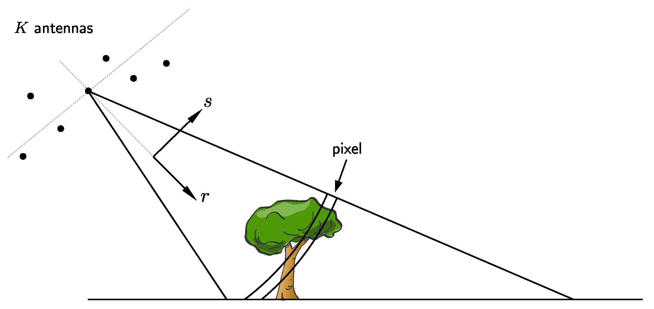
2. TomoSAR Principles
2.1. Signal Model
2.2. 3-D Imaging by Tomographic Inversion
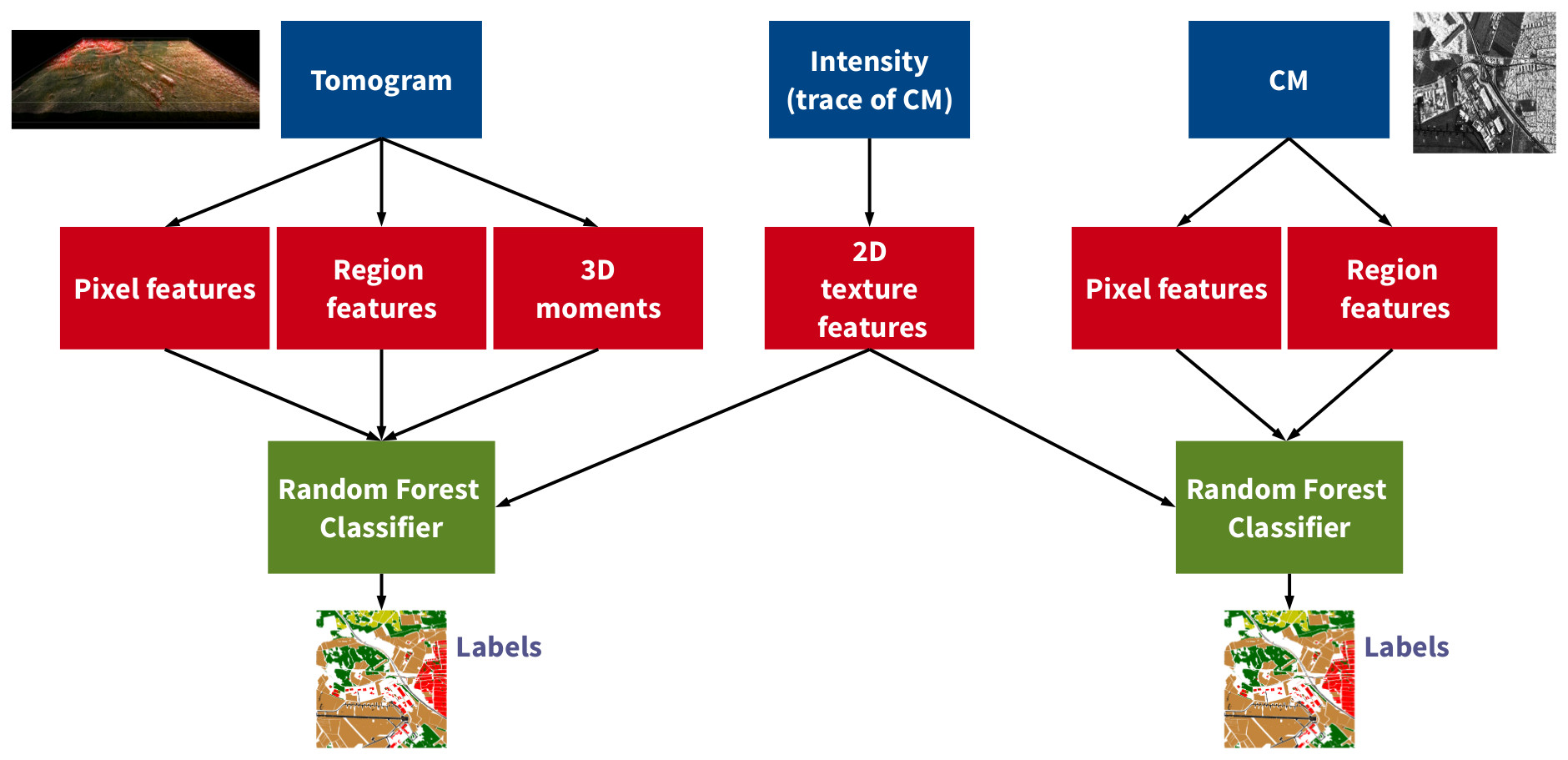
3. Feature Extraction Methodology
3.1. Pixel-Based Features
3.1.1. Covariance-Based Features
3.1.2. Tomogram-Based Features
3.2. Spatial Features
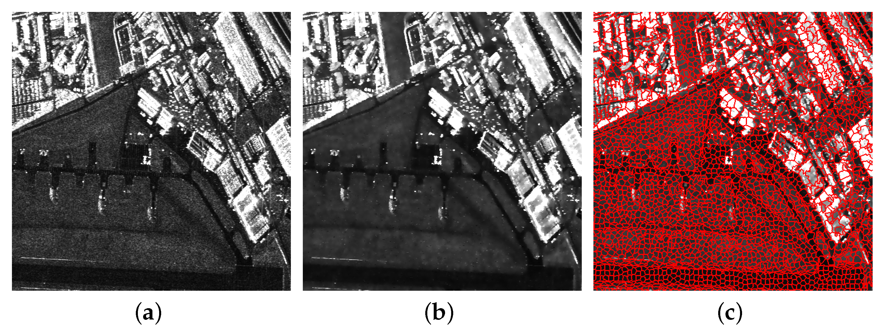
3.2.1. Region Features
3.2.2. Texture Features
3.2.3. 3-D Descriptors
3.3. Random Forest Classifier
4. Experiments
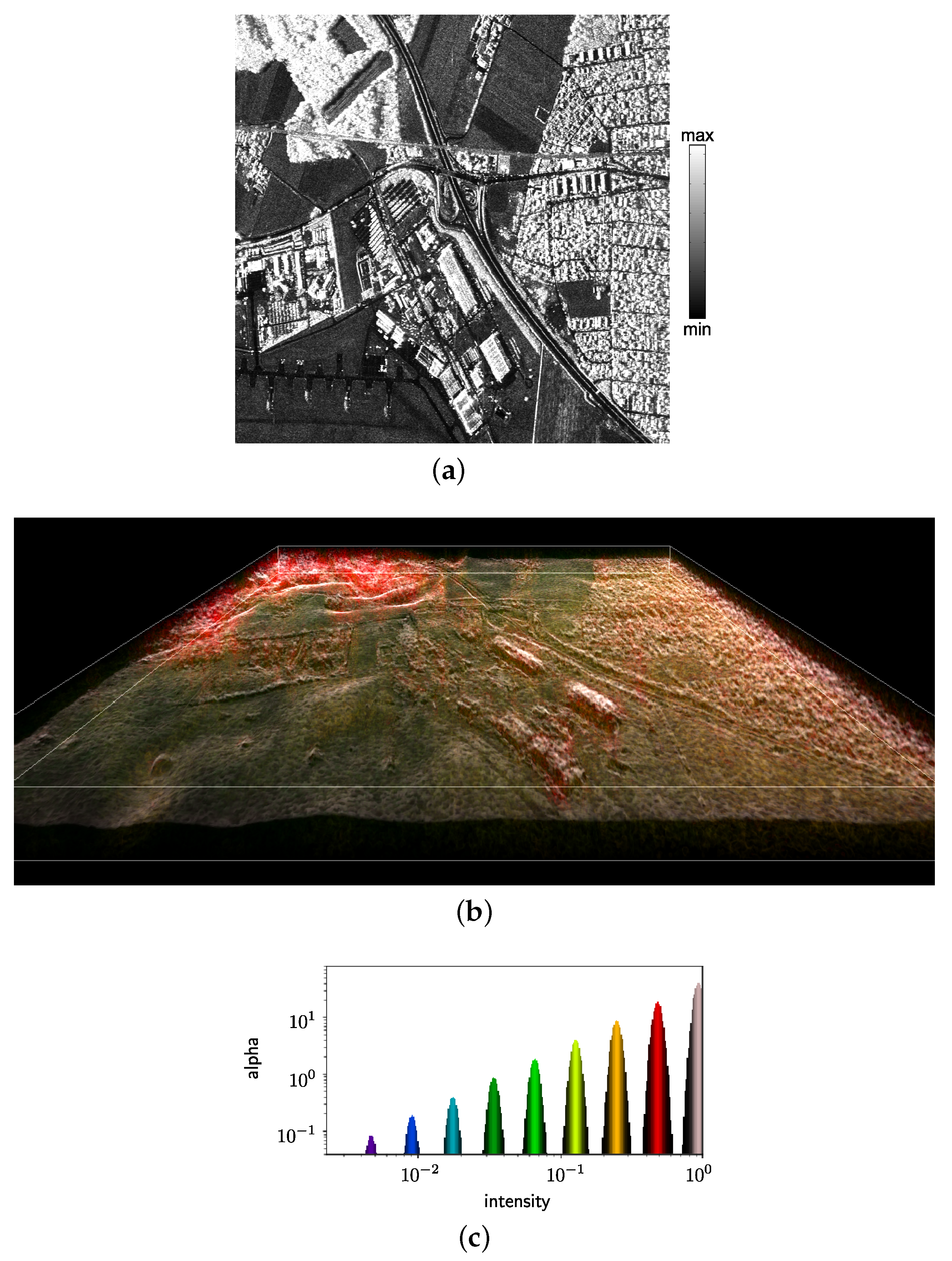
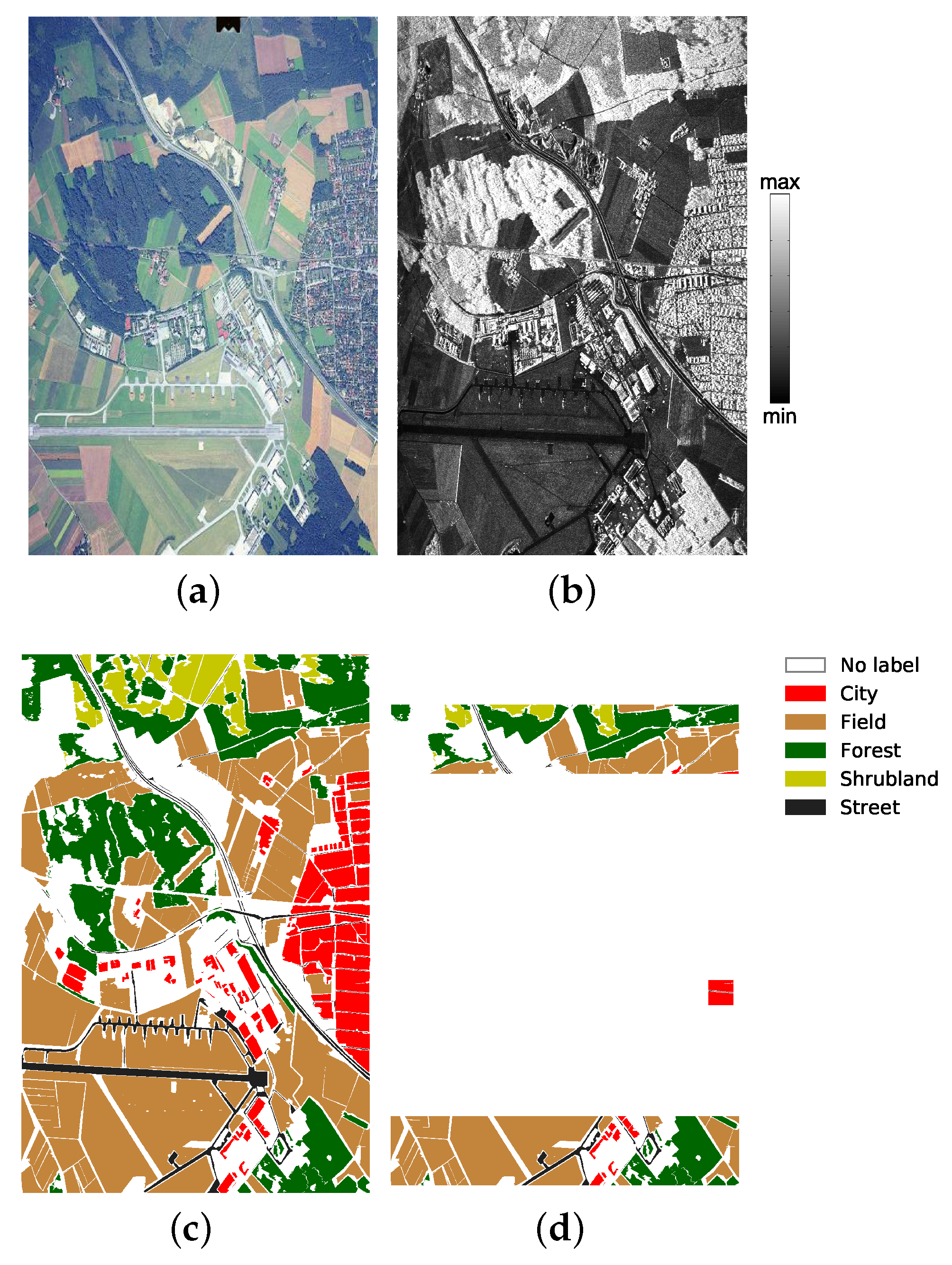
4.1. Data
4.2. Description of the Feature Subsets
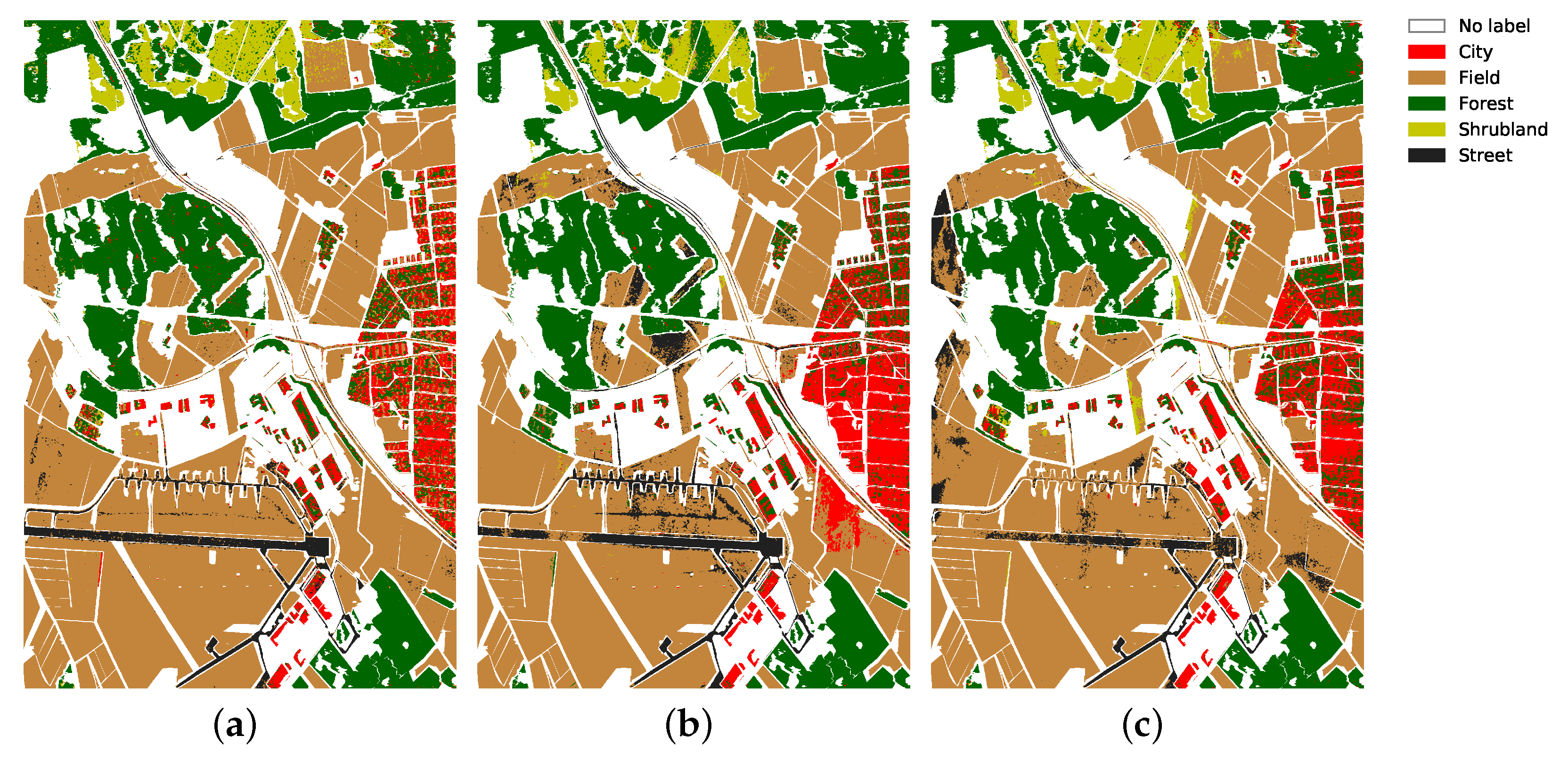
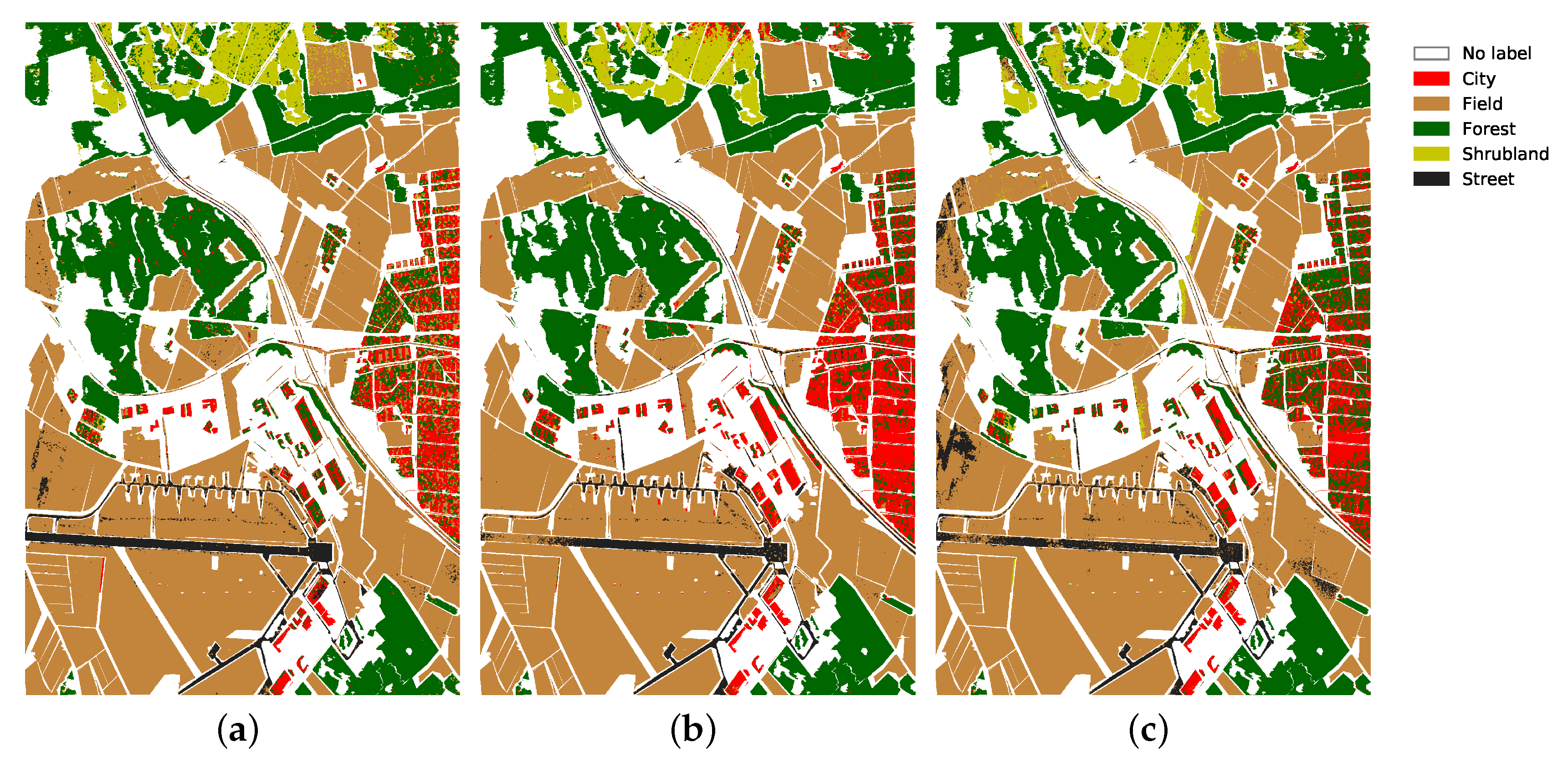
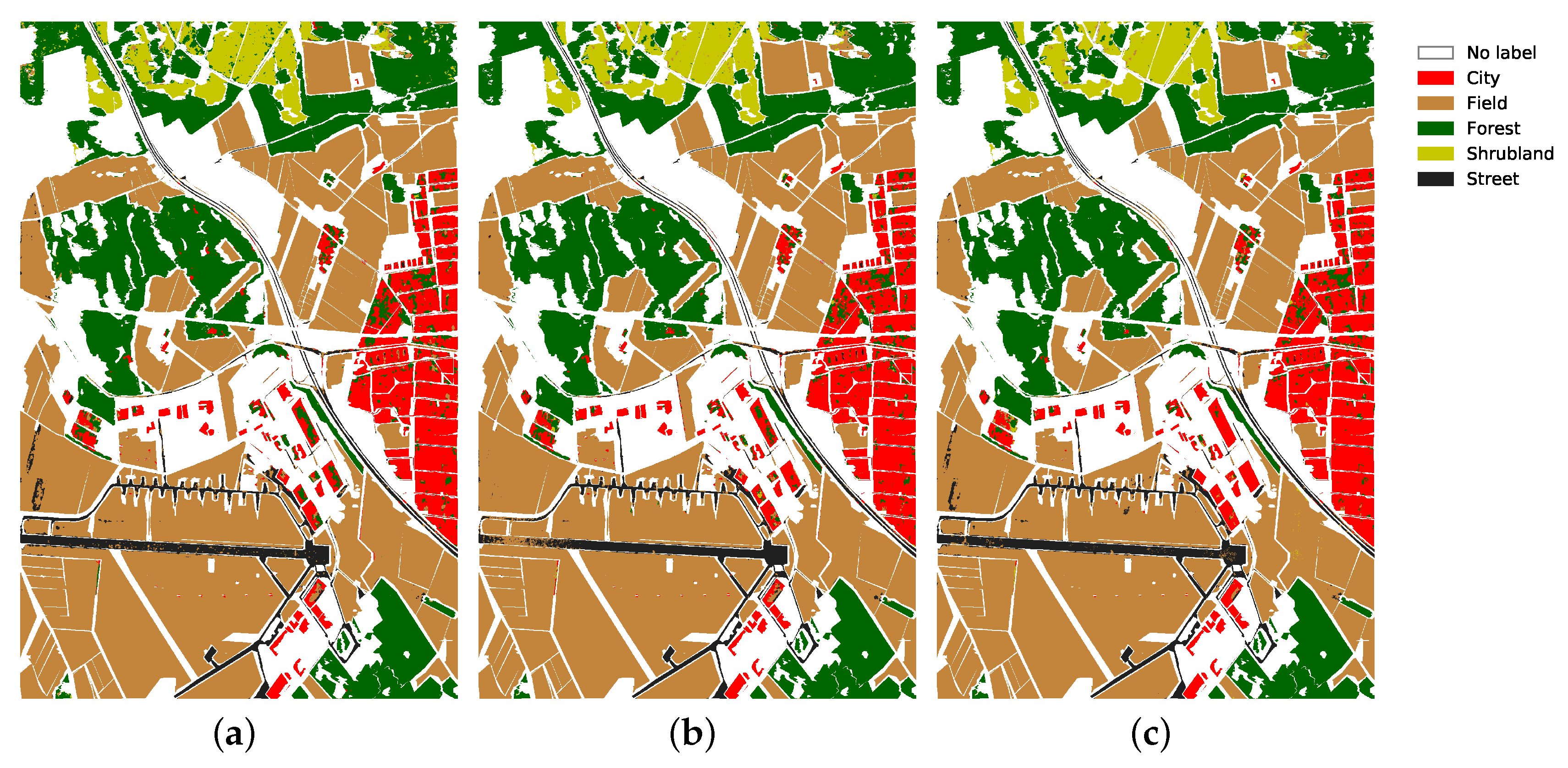
4.3. Results
5. Discussion
6. Conclusions
Author Contributions
Funding
Acknowledgments
Conflicts of Interest
References
- Herold, N.D.; Haack, B.N.; Solomon, E. An evaluation of radar texture for land use/cover extraction in varied landscapes. Int. J. Appl. Earth Obs. Geoinform. 2004, 5, 113–128. [Google Scholar] [CrossRef]
- Cloude, S.; Pottier, E. A review of target decomposition theorems in radar polarimetry. IEEE Trans. Geosci. Remote Sens. 1996, 34, 498–518. [Google Scholar] [CrossRef]
- Touzi, R. Polarimetric target scattering decomposition: A review. In Proceedings of the 2016 IEEE International Geoscience and Remote Sensing Symposium (IGARSS), Beijing, China, 10–15 July 2016; pp. 5658–5661. [Google Scholar]
- Lee, J.S.; Grunes, M.; Pottier, E. Quantitative comparison of classification capability: Fully polarimetric versus dual and single-polarization SAR. IEEE Trans. Geosci. Remote Sens. 2001, 39, 2343–2351. [Google Scholar]
- Corr, D.; Cloude, S.; Ferro-Famil, L.; Hoekman, D.; Partingon, K.; Pottier, E.; Rodrigues, A. A review of the applications of SAR polarimetric interferometry—An ESA funded study. In Proceedings of the POLinSAR 2003, Frascati, Italy, 14–16 January 2003. [Google Scholar]
- Borghys, D.; Perneel, C. A supervised classification of multi-channel high-resolution SAR data. Proc. Earsel 2007, 6, 26–37. [Google Scholar]
- Feng, J.; Cao, Z.; Pi, Y. Polarimetric Contextual Classification of PolSAR Images Using Sparse Representation and Superpixels. Remote Sens. 2014, 6, 7158–7181. [Google Scholar] [CrossRef]
- Liu, H.; Zhu, D.; Yang, S.; Hou, B.; Gou, S.; Xiong, T.; Jiao, L. Semisupervised Feature Extraction With Neighborhood Constraints for Polarimetric SAR Classification. IEEE J. Sel. Top. Appl. Earth Obs. Remote Sens. 2016, 9, 3001–3015. [Google Scholar] [CrossRef]
- Hänsch, R. Generic Object Categorization in PolSAR Images- and Beyond. Ph.D. Thesis, TU Berlin, Berlin, Germany, 2014. [Google Scholar]
- Hänsch, R.; Hellwich, O. Skipping the real world: Classification of PolSAR images without explicit feature extraction. ISPRS J. Photogramm. Remote Sens. 2018, 140, 122–132. [Google Scholar] [CrossRef]
- Hänsch, R.; Hellwich, O. Complex-Valued Convolutional Neural Networks for Object Detection in PolSAR data. In Proceedings of the 8th European Conference on Synthetic Aperture Radar, Aachen, Germany, 7–10 June 2010; pp. 1–4. [Google Scholar]
- Zhou, Y.; Wang, H.; Xu, F.; Jin, Y.Q. Polarimetric SAR Image Classification Using Deep Convolutional Neural Networks. IEEE Geosci. Remote Sens. Lett. 2016, 13, 1935–1939. [Google Scholar] [CrossRef]
- Yang, M.S.; Moon, W.M. Decision level fusion of multi-frequency polarimetric SAR and optical data with Dempster-Shafer evidence theory. In Proceedings of the 2003 IEEE International Geoscience and Remote Sensing Symposium (IGARSS 2003), Toulouse, France, 21–25 July 2003; Volume 6, pp. 3668–3670. [Google Scholar]
- Hagensieker, R.; Waske, B. Evaluation of Multi-Frequency SAR Images for Tropical Land Cover Mapping. Remote Sens. 2018, 10, 257. [Google Scholar] [CrossRef]
- Tupin, F.; Houshmand, B.; Datcu, M. Road detection in dense urban areas using SAR imagery and the usefulness of multiple views. IEEE Trans. Geosci. Remote Sens. 2002, 40, 2405–2414. [Google Scholar] [CrossRef]
- Su, X.; Deledalle, C.; Tupin, F.; Sun, H. Change detection and classification of multi-temporal SAR series based on generalized likelihood ratio comparing-and-recognizing. In Proceedings of the 2014 IEEE Geoscience and Remote Sensing Symposium, Quebec City, QC, Canada, 13–18 July 2014; pp. 1433–1436. [Google Scholar]
- Lin, K.F.; Perissin, D. Single-Polarized SAR Classification Based on a Multi-Temporal Image Stack. Remote Sens. 2018, 10, 1087. [Google Scholar] [CrossRef]
- Reigber, A.; Neumann, M.; Guillaso, S.; Sauer, S.; Ferro-Famil, L. Evaluating PolInSAR parameter estimation using tomographic imaging results. In Proceedings of the European Radar Conference, EURAD 2005, Paris, France, 3–4 October 2005; pp. 189–192. [Google Scholar] [CrossRef]
- Vasile, G.; Trouvé, E.; Valet, L.; Nicolas, J.; Gay, M.; Bombrun, L.; Bolon, P. Feature detection in PolInSAR images by an interactive fuzzy fusion approach. Application to glacier monitoring. In Proceedings of the 3rd International Workshop on Science and Applications of SAR Polarimetry and Polarimetric Interferometry, Frascati, Italy, 22–26 January 2007. [Google Scholar]
- Shimoni, M.; Borghys, D.; Heremans, R.; Perneel, C.; Acheroy, M. Fusion of PolSAR and PolInSAR data for land cover classification. Int. J. Appl. Earth Obs. Geoinform. 2009, 11, 169–180. [Google Scholar] [CrossRef]
- Reigber, A.; Moreira, A. First demonstration of airborne SAR tomography using multibaseline L-band data. IEEE Trans. Geosci. Remote Sens. 2000, 38, 2142–2152. [Google Scholar] [CrossRef]
- Tebaldini, S. Single and Multipolarimetric SAR Tomography of Forested Areas: A Parametric Approach. IEEE Trans. Geosci. Remote Sens. 2010, 48, 2375–2387. [Google Scholar] [CrossRef]
- Aguilera, E.; Nannini, M.; Reigber, A. Wavelet-Based Compressed Sensing for SAR Tomography of Forested Areas. IEEE Trans. Geosci. Remote Sens. 2013, 51, 5283–5295. [Google Scholar] [CrossRef]
- Banda, F.; Dall, J.; Tebaldini, S. Single and Multipolarimetric P-Band SAR Tomography of Subsurface Ice Structure. IEEE Trans. Geosci. Remote Sens. 2016, 54, 2832–2845. [Google Scholar] [CrossRef]
- Zhu, X.X.; Bamler, R. Demonstration of Super-Resolution for Tomographic SAR Imaging in Urban Environment. IEEE Trans. Geosci. Remote Sens. 2012, 50, 3150–3157. [Google Scholar] [CrossRef]
- Shahzad, M.; Zhu, X.X. Automatic Detection and Reconstruction of 2-D/3-D Building Shapes From Spaceborne TomoSAR Point Clouds. IEEE Trans. Geosci. Remote Sens. 2016, 54, 1292–1310. [Google Scholar] [CrossRef]
- Ley, A.; D’Hondt, O.; Hellwich, O. Regularization and Completion of TomoSAR Point Clouds in a Projected Height Map Domain. IEEE Int. Geosci. Remote Sens. Symp. 2017, 11, 5854–5857. [Google Scholar]
- D’Hondt, O.; Guillaso, S.; Hellwich, O. Geometric primitive extraction for 3D reconstruction of urban areas from tomographic SAR data. In Proceedings of the Joint Urban Remote Sensing Event (JURSE), Sao Paulo, Brazil, 21–23 April 2013; pp. 206–209. [Google Scholar] [CrossRef]
- D’Hondt, O.; Guillaso, S.; Hellwich, O. Automatic extraction of geometric structures for 3D reconstruction from tomographic SAR data. In Proceedings of the 2012 IEEE International Geoscience and Remote Sensing Symposium, Munich, Germany, 22–27 July 2012; pp. 3728–3731. [Google Scholar] [CrossRef]
- Shahzad, M.; Zhu, X.X. Robust Reconstruction of Building Facades for Large Areas Using Spaceborne TomoSAR Point Clouds. IEEE Trans. Geosci. Remote Sens. 2015, 53, 752–769. [Google Scholar] [CrossRef]
- Cazcarra-Bes, V.; Tello-Alonso, M.; Fischer, R.; Heym, M.; Papathanassiou, K. Monitoring of Forest Structure Dynamics by Means of L-Band SAR Tomography. Remote Sens. 2017, 9, 1229. [Google Scholar] [CrossRef]
- D’Hondt, O.; Hänsch, R.; Hellwich, O. Supervised classification from TomoSAR data. In Proceedings of the 12th European Conference on Synthetic Aperture Radar, Aachen, Germany, 4–7 June 2018. [Google Scholar]
- D’Hondt, O.; Hänsch, R.; Hellwich, O. Feature Design for Classification from TomoSAR Data. In Proceedings of the IGARSS 2018, Valencia, Spain, 22–27 July 2018. [Google Scholar]
- D’Hondt, O.; López-Martínez, C.; Guillaso, S.; Hellwich, O. Nonlocal Filtering Applied to 3-D Reconstruction of Tomographic SAR Data. IEEE Trans. Geosci. Remote Sens. 2018, 56, 272–285. [Google Scholar] [CrossRef]
- Stoica, P.; Moses, R. Spectral Analysis of Signals; Pearson Prentice Hall: Upper Saddle River, NJ, USA, 2005. [Google Scholar]
- Budillon, A.; Evangelista, A.; Schirinzi, G. Three-Dimensional SAR Focusing From Multipass Signals Using Compressive Sampling. IEEE Trans. Geosci. Remote Sens. 2011, 49, 488–499. [Google Scholar] [CrossRef]
- Turk, M.J.; Smith, B.D.; Oishi, J.S.; Skory, S.; Skillman, S.W.; Abel, T.; Norman, M.L. yt: A Multi-code Analysis Toolkit for Astrophysical Simulation Data. Astrophys. J. Suppl. Ser. 2011, 192, 9. [Google Scholar] [CrossRef]
- Zebker, H.A.; Villasenor, J. Decorrelation in interferometric radar echoes. IEEE Trans. Geosci. Remote Sens. 1992, 30, 950–959. [Google Scholar] [CrossRef]
- Luo, X.; Askne, J.; Smith, G.; Dammert, P. Coherence Characteristics of Radar Signals From Rough Soil. J. Electromagn. Waves Appl. 2000, 14, 1555–1557. [Google Scholar] [CrossRef]
- Achanta, R.; Shaji, A.; Smith, K.; Lucchi, A.; Fua, P.; Süsstrunk, S. SLIC Superpixels Compared to State-of-the-art Superpixel Methods. IEEE Trans. Pattern Anal. Mach. Intell. 2012, 34, 2274–2282. [Google Scholar] [CrossRef] [PubMed]
- Haralick, R.; Shanmugam, K.; Dinstein, I. Textural Features for Image Classification. IEEE Trans. Syst. Man Cybern. 1973, 3, 610–621. [Google Scholar] [CrossRef]
- Bovik, A.; Clarke, M.; Geisler, W. Multichannel Texture Analysis Using Localized Spatial Filters. IEEE Trans. Pattern Anal. Mach. Intell. 1990, 12, 55–73. [Google Scholar] [CrossRef]
- Bigun, J.; Granlund, G.H. Optimal orientation detection of linear symmetry. In Proceedings of the First International Conference on Computer Vision (ICCV), London, UK, 8–11 June 1987; IEEE Computer Society Press: Los Alamitos, CA, USA, 1987; pp. 433–438. [Google Scholar]
- Breiman, L. Random Forests. Machine Learn. 2001, 45, 5–32. [Google Scholar] [CrossRef]
- Reigber, A. Airborne Polarimetric SAR Tomography. Ph.D. Thesis, University of Stuttgart, Stuttgart, Germany, 2001. [Google Scholar]
- Lee, J.S.; Grunes, M.R.; Kwok, R. Classification of multi-look polarimetric SAR imagery based on complex Wishart distribution. Int. J. Remote Sens. 1994, 15, 2299–2311. [Google Scholar] [CrossRef]
- Jager, M.; Neumann, M.; Guillaso, S.; Reigber, A. A Self-Initializing PolInSAR Classifier Using Interferometric Phase Differences. IEEE Trans. Geosci. Remote Sens. 2007, 45, 3503–3518. [Google Scholar] [CrossRef]
- Ferro-Famil, L.; Kugler, F.; Potier, E.; Lee, J.S. Forest Mapping and Classification at L-Band using Pol-InSAR Optimal Coherence Set Statistics. In Proceedings of the EUSAR 2006, Dresden, Germany, 16–18 May 2006; pp. 1–4. [Google Scholar]
- Singh, J.; Datcu, M. SAR Image Categorization With Log Cumulants of the Fractional Fourier Transform Coefficients. IEEE Trans. Geosci. Remote Sens. 2013, 51, 5273–5282. [Google Scholar] [CrossRef]


| Tomographic CM | |
|---|---|
| raw | Real and imaginary part of all elements of the TomoSAR CM. |
| TCM1 | Diagonal elements of the TomoSAR CM (Section 3.1.1). |
| TCM2 | TCM1 + Coherences extracted from the TomoSAR CM (Section 3.1.1). |
| TCM3 | TCM2 + Region-based features of intensity (Section 3.2.1). |
| TCM4 | TCM3 + Patch features (Section 3.2.2). |
| Tomograms | |
| raw | All entries of the tomogram. |
| TGR1 | Pixel-based features (Section 3.1.2). |
| TGR2 | TGR1 + Region-based features of intensity (Section 3.2.1). |
| TGR3 | TGR2 + Patch features (Section 3.2.2). |
| TGR4 | TGR3 + Region features of tomograms (Section 3.2.1). |
| TGR5 | TGR4 + 3-D features (Section 3.2.3). |
| Polarimetric CM | |
| raw | Real and imaginary part of all elements of the PolSAR CM. |
| PCM1 | Diagonal elements of the PolSAR CM (Section 3.1.1). |
| PCM2 | PCM1 + Coherences extracted from the PolSAR CM (Section 3.1.1). |
| PCM3 | PCM2 + Relative phases extracted from the PolSAR CM (Section 3.1.1). |
| PCM4 | PCM3 + Region-based features of intensity (Section 3.2.1). |
| PCM5 | PCM4 + Patch features (Section 3.2.2). |
| City | Field | Forest | Shrubland | Street | OA | BA | Num. Feat. | |
|---|---|---|---|---|---|---|---|---|
| Raw | 51.8 | 98.2 | 96.8 | 81.9 | 58.2 | 87.4 | 77.4 | 9 |
| PCM1 | 39.4 | 97.7 | 95.6 | 80.3 | 54.4 | 84.7 | 73.5 | 3 |
| PCM2 | 48.0 | 97.8 | 96.6 | 82.6 | 56.2 | 86.5 | 76.2 | 6 |
| PCM3 | 52.4 | 98.1 | 96.9 | 82.3 | 60.5 | 87.6 | 78.0 | 9 |
| PCM4 | 79.6 | 98.7 | 97.2 | 84.3 | 70.8 | 93.0 | 86.1 | 13 |
| PCM5 | 81.9 | 98.8 | 97.7 | 84.5 | 78.4 | 93.9 | 88.3 | 134 |
| City | Field | Forest | Shrubland | Street | OA | BA | Num. Feat. | |
|---|---|---|---|---|---|---|---|---|
| Raw | 64.3 | 89.6 | 99.1 | 52.6 | 60.7 | 84.0 | 73.3 | 100 |
| TCM1 | 28.2 | 97.2 | 96.9 | 64.1 | 56.4 | 82.2 | 68.6 | 10 |
| TCM2 | 69.2 | 98.7 | 98.4 | 73.8 | 61.8 | 90.5 | 80.4 | 55 |
| TCM3 | 83.5 | 99.2 | 99.2 | 82.5 | 70.6 | 94.1 | 87.0 | 59 |
| TCM4 | 85.2 | 99.3 | 99.2 | 85.3 | 74.9 | 94.9 | 88.8 | 180 |
| City | Field | Forest | Shrubland | Street | OA | BA | Num. Feat. | |
|---|---|---|---|---|---|---|---|---|
| Raw | 61.5 | 92.4 | 98.7 | 75.1 | 39.1 | 84.8 | 73.4 | 200 |
| TGR1 | 48.3 | 95.1 | 99.1 | 75.0 | 54.4 | 85.2 | 74.4 | 36 |
| TGR2 | 83.5 | 98.8 | 99.4 | 79.2 | 70.0 | 93.8 | 86.2 | 40 |
| TGR3 | 85.5 | 98.7 | 99.4 | 84.6 | 78.3 | 94.8 | 89.3 | 161 |
| TGR4 | 87.3 | 98.9 | 99.4 | 85.6 | 79.3 | 95.3 | 90.1 | 169 |
| TGR5 | 88.0 | 98.8 | 99.5 | 87.7 | 78.9 | 95.5 | 90.6 | 186 |
| City | Field | Forest | Shrubland | Street | OA | BA | Num. Feat. | |
|---|---|---|---|---|---|---|---|---|
| TCM2b | 72.8 | 96.1 | 99.0 | 62.4 | 53.4 | 88.8 | 76.7 | 100 |
| TCM3b | 85.0 | 98.3 | 99.3 | 76.3 | 57.1 | 92.8 | 83.2 | 104 |
| TCM4b | 86.0 | 99.0 | 99.2 | 82.7 | 66.8 | 94.3 | 86.7 | 225 |
| City | Field | Forest | Shrubland | Street | OA | BA | |
|---|---|---|---|---|---|---|---|
| PolSAR CM | 28.8 | 78.7 | 78.3 | 96.0 | 80.5 | 71.8 | 72.5 |
| TomoSAR CM | 43.3 | 42.8 | 94.4 | 89.0 | 88.1 | 59.1 | 71.5 |
© 2018 by the authors. Licensee MDPI, Basel, Switzerland. This article is an open access article distributed under the terms and conditions of the Creative Commons Attribution (CC BY) license (http://creativecommons.org/licenses/by/4.0/).
Share and Cite
D’Hondt, O.; Hänsch, R.; Wagener, N.; Hellwich, O. Exploiting SAR Tomography for Supervised Land-Cover Classification. Remote Sens. 2018, 10, 1742. https://doi.org/10.3390/rs10111742
D’Hondt O, Hänsch R, Wagener N, Hellwich O. Exploiting SAR Tomography for Supervised Land-Cover Classification. Remote Sensing. 2018; 10(11):1742. https://doi.org/10.3390/rs10111742
Chicago/Turabian StyleD’Hondt, Olivier, Ronny Hänsch, Nicolas Wagener, and Olaf Hellwich. 2018. "Exploiting SAR Tomography for Supervised Land-Cover Classification" Remote Sensing 10, no. 11: 1742. https://doi.org/10.3390/rs10111742
APA StyleD’Hondt, O., Hänsch, R., Wagener, N., & Hellwich, O. (2018). Exploiting SAR Tomography for Supervised Land-Cover Classification. Remote Sensing, 10(11), 1742. https://doi.org/10.3390/rs10111742