A Novel Method of Generating Deformation Time-Series Using Interferometric Synthetic Aperture Radar and Its Application in Mexico City


Abstract
1. Introduction
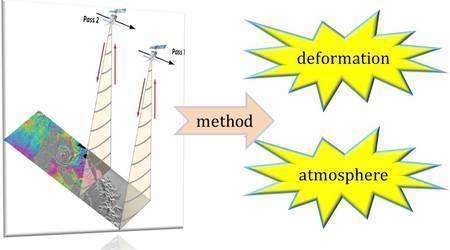
2. Method
2.1. Data Preprocessing
2.2. Mathematical Model
3. Study Area and Datasets
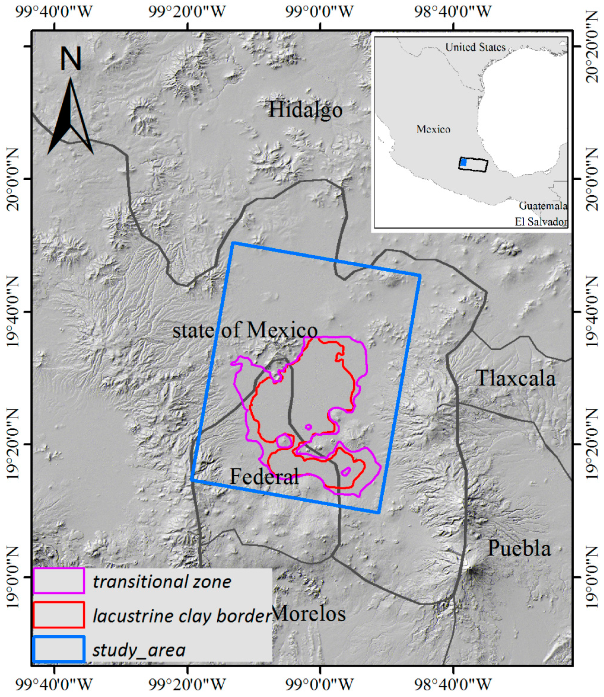
3.1. Geological Background
3.2. Data Processing
4. Experimental Results and Analysis
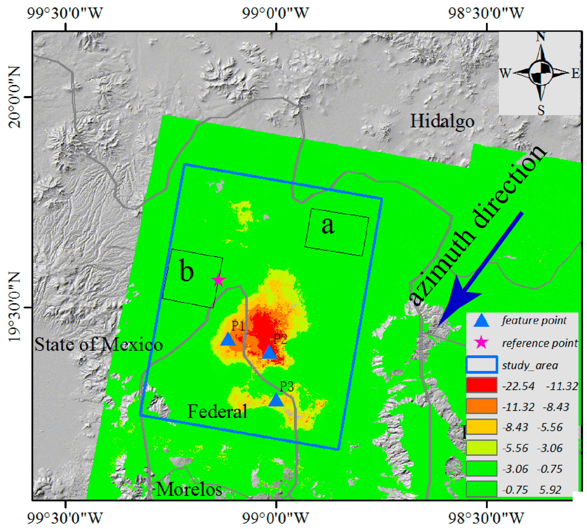
4.1. Annual Velocity
4.2. Mathematical Model
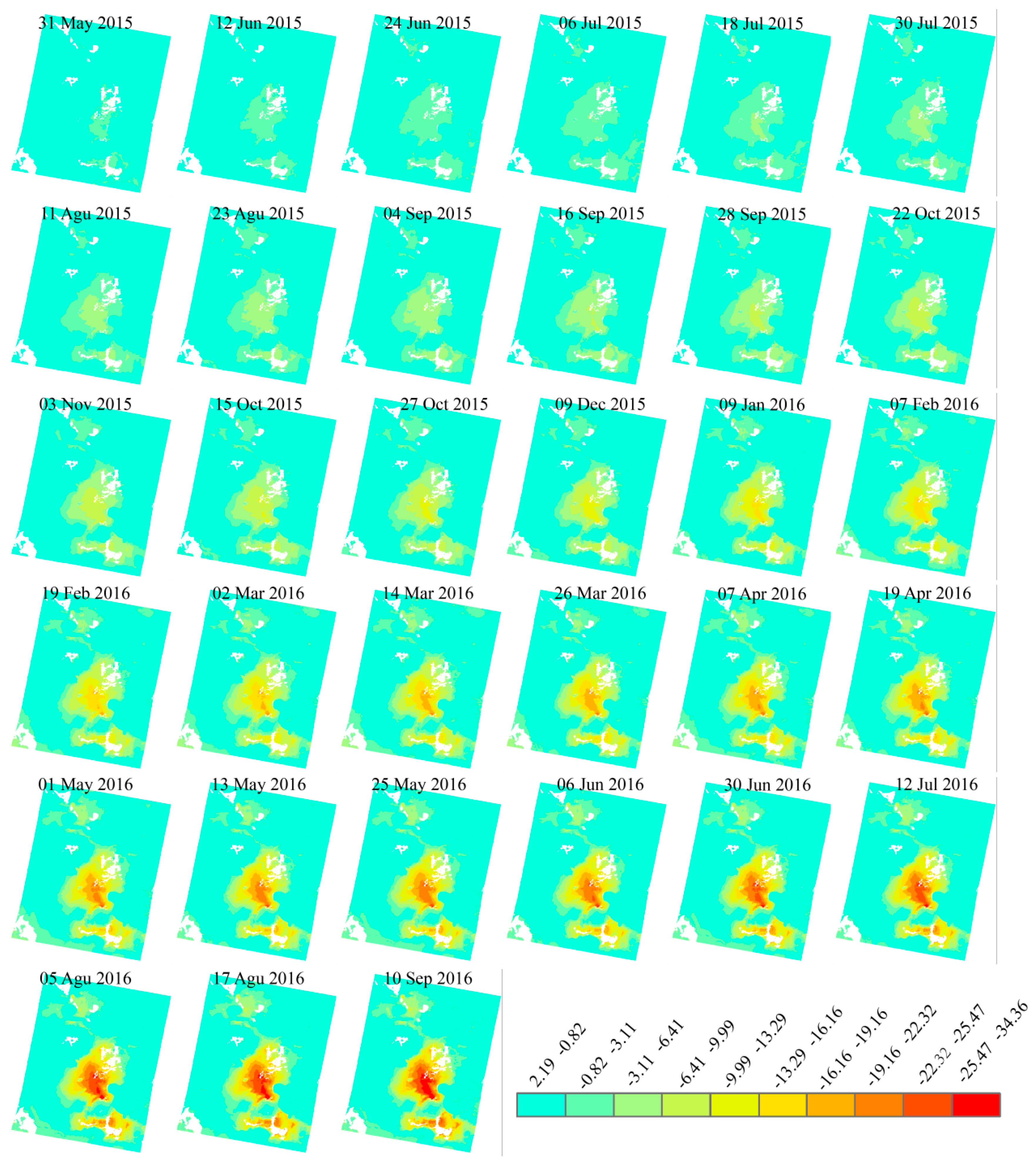
4.3. Time-Series Deformation
4.4. Atmospheric and Nonlinear Results
5. Discussion
5.1. Mathematical Models
5.2. Spatio-Temporal Changes of the Deformation in Mexico City
6. Conclusions
Author Contributions
Funding
Acknowledgments
Conflicts of Interest
References
- Tomás, R.; Li, Z. Earth Observations for Geohazards: Present and Future Challenges. Remote Sens. 2017, 9, 194. [Google Scholar] [CrossRef]
- Cui, Z.D. Land Subsidence Disaster caused by Natural Factors and Human Activities. Disaster Adv. 2012, 5, 3–4. [Google Scholar]
- Qu, F.; Zhang, Q.; Lu, Z.; Zhao, C.; Yang, C.; Zhang, J. Land subsidence and ground fissures in Xi’an, China 2005–2012 revealed by multi-band InSAR time-series analysis. Remote Sens. Environ. 2014, 155, 366–376. [Google Scholar] [CrossRef]
- Julio-Miranda, P.; Ortíz-Rodríguez, A.J.; Palacio-Aponte, A.G.; López-Doncel, R.; Barboza-Gudiño, R. Damage assessment associated with land subsidence in the San Luis Potosi-Soledad de Graciano Sanchez metropolitan area, Mexico, elements for risk management. Nat. Hazards 2012, 64, 751–765. [Google Scholar] [CrossRef]
- Prati, C.; Ferretti, A.; Perissin, D. Recent advances on surface ground deformation measurement by means of repeated space-borne SAR observations. J. Geodyn. 2010, 49, 161–170. [Google Scholar] [CrossRef]
- Crosetto, M.; Crippa, B.; Monserrat, O.; Agudo, M.; Biescas, E. Land Subsidence Measurement with SAR Interferometric Data. In Proceedings of the ENVISAT Symposium 2004, Salzburg, Austria, 6–10 September 2004. [Google Scholar]
- Sneed, M.; Stork, S.V.; Ikehara, M.E. Detection and Measurement of Land Subsidence Using Global Positioning System and Interferometric Synthetic Aperture Radar, Coachella Valley, California, 1998–2000; Water-Resources Investigations Report; U.S. Geological Survey: Sacramento, CA, USA, 2002; Volume 8, Suppl. 1.
- Ciampalini, A.; Bardi, F.; Bianchini, S.; Frodella, W.; Ventisette, C.D.; Moretti, S.; Casagli, N. Analysis of building deformation in landslide area using multisensor PSInSAR™ technique. Int. J. Appl. Earth Obs. Geoinf. 2014, 33, 166–180. [Google Scholar] [CrossRef] [PubMed]
- Attema, E.; Snoeij, P.; Torres, R.; Pietropaolo, A. Analysis of Sentinel-1 Mission Capabilities. In Proceedings of the 2009 IEEE International Geoscience and Remote Sensing Symposium, Cape Town, South Africa, 12–17 July 2009; pp. 1–4. [Google Scholar]
- Massonnet, D.; Rossi, M.; Carmona, C.; Adragna, F.; Peltzer, G.; Feigl, K.; Rabaute, T. The displacement field of the Landers earthquake mapped by radar interferometry. Nat. Int. Wkl. J. Sci. 1993, 364, 138–142. [Google Scholar] [CrossRef]
- Sandwell, D.T.; Sichoix, L.; Agnew, D.; Bock, Y.; Minster, J.B. Near real-time radar interferometry of the Mw 7.1 Hector Mine Earthquake. Geophys. Res. Lett. 2000, 27, 3101–3104. [Google Scholar] [CrossRef]
- Strozzi, T.; Wegmuller, U.; Werner, C.L.; Wiesmann, A. JERS SAR interferometry for land subsidence monitoring. IEEE Trans. Geosci. Remote Sens. 2003, 41, 1702–1708. [Google Scholar] [CrossRef]
- Zebker, H.A.; Rosen, P.A.; Goldstein, R.M.; Gabriel, A.; Werner, C.L. On the derivation of coseismic displacement fields using differential radar interferometry: The Landers earthquake. J. Geophys. Res. Solid Earth 2002, 99, 19617–19634. [Google Scholar] [CrossRef]
- Liu, G.X.; Ding, X.L.; Li, Z.L.; Li, Z.W.; Chen, Y.Q.; Yu, S.B. Pre- and co-seismic ground deformations of the 1999 Chi-Chi, Taiwan earthquake, measured with SAR interferometry. Comput. Geosci. 2004, 30, 333–343. [Google Scholar] [CrossRef]
- Yang, C.; Zhang, Q.; Xu, Q.; Zhao, C.; Peng, J.; Ji, L.; Yang, C.; Zhang, Q.; Xu, Q.; Zhao, C. Complex Deformation Monitoring over the Linfen–Yuncheng Basin (China) with Time Series InSAR Technology. Remote Sens. 2016, 8, 284. [Google Scholar] [CrossRef]
- Zhao, C.; Lu, Z.; Zhang, Q. Time-series deformation monitoring over mining regions with SAR intensity-based offset measurements. Remote Sens. Lett. 2013, 4, 436–445. [Google Scholar] [CrossRef]
- Zebker, H.A.; Villasenor, J. Decorrelation in interferometric radar echoes. IEEE Trans. Geosci. Remote Sens. 1992, 30, 950–959. [Google Scholar] [CrossRef]
- Hanssen, R.; Feijt, A. A First Quantitative Evaluation of Atmospheric Effects on SAR Interferometry. ESA SAR Interferom. 1997, 406, 277. [Google Scholar]
- Emardson, T.R.; Simons, M.; Webb, F.H. Neutral atmospheric delay in interferometric synthetic aperture radar applications: Statistical description and mitigation. J. Geophys. Res. Solid Earth 2003, 108, 241–258. [Google Scholar] [CrossRef]
- Reuter, H.I.; Nelson, A.; Jarvis, A. An evaluation of void-filling interpolation methods for SRTM data. Int. J. Geogr. Inf. Sci. 2007, 21, 983–1008. [Google Scholar] [CrossRef]
- Hooper, A.; Bekaert, D.; Spaans, K.; Arıkan, M. Recent advances in SAR interferometry time series analysis for measuring crustal deformation. Tectonophysics 2012, 514, 1–13. [Google Scholar] [CrossRef]
- Berardino, P.; Fornaro, G.; Lanari, R.; Sansosti, E. A new algorithm for surface deformation monitoring based on small baseline differential SAR interferograms. IEEE Trans. Geosci. Remote Sens. 2002, 40, 2375–2383. [Google Scholar] [CrossRef]
- Usai, S. A New Approach for Longterm Monitoring of Deformations by Differential SAR Interferometry; Delft University Press: Delft, The Netherlands, 2001. [Google Scholar]
- Lanari, R.; Casu, F.; Manzo, M.; Zeni, G.; Berardino, P.; Manunta, M.; Pepe, A. An Overview of the Small BAseline Subset Algorithm: A DInSAR Technique for Surface Deformation Analysis. Pure Appl. Geophys. 2007, 164, 637–661. [Google Scholar] [CrossRef]
- Lauknes, T.R.; Zebker, H.A.; Larsen, Y. InSAR deformation time series using an L1-Norm small-baseline approach. IEEE Trans. Geosci. Remote Sens. 2011, 49, 536–546. [Google Scholar] [CrossRef]
- Hooper, A.; Zebker, H.; Segall, P.; Kampes, B. A new method for measuring deformation on volcanoes and other natural terrains using InSAR persistent scatterers. Geophys. Res. Lett. 2004, 31, 1–5. [Google Scholar] [CrossRef]
- Zhang, L. Temporarily Coherent Point SAR Interferometry. Ph.D. Thesis, Hong Kong Polytechnic University, Hong Kong, China, 2012. [Google Scholar]
- Vega, F.G.E. Subsidence of the City of Mexico: A Historical Review. 1976. Available online: http://hydrologie.org/redbooks/a121/iahs_121_0035.pdf (accessed on 25 September 2018).
- Strozzi, T.; Wegmuller, U. Land subsidence in Mexico City mapped by ERS differential SAR interferometry. In Proceedings of the IEEE 1999 International Geoscience and Remote Sensing Symposium (IGARSS 1999), Hamburg, Germany, 28 June–2 July 1999; Volume 1944, pp. 1940–1942. [Google Scholar]
- Cabralcano, E.; Dixon, T.H.; Miralleswilhelm, F.; Diazmolina, O.; Sanchezzamora, O.; Carande, R.E. Space geodetic imaging of rapid ground subsidence in Mexico City. Geol. Soc. Am. Bull. 2008, 120, 1556–1566. [Google Scholar] [CrossRef]
- Osmanoglu, B.; Dixon, T.H.; Wdowinski, S.; Cabralcano, E. Mexico City subsidence observed with PS-InSAR. Int. J. Appl. Earth Obs. Geoinf. 2011, 13, 1–12. [Google Scholar] [CrossRef]
- Chaussard, E.; Wdowinski, S.; Cabral-Cano, E.; Amelung, F. Land subsidence in central Mexico detected by ALOS InSAR time-series. Remote Sens. Environ. 2014, 140, 94–106. [Google Scholar] [CrossRef]
- Solano-Rojas, D.; Cabral-Cano, E.; Hernández-Espriú, A.; Wdowinski, S.; Demets, C.; Salazar-Tlaczani, L.; Falorni, G.; Bohane, A. The relationship of InSAR-GPS land subsidence and the groundwater level decrease in wells of the Mexico City Metropolitan Area. Bol. Soc. Geol. Mex. 2015, 67, 273–283. [Google Scholar]
- Sowter, A.; Bin Che Amat, M.; Cigna, F.; Marsh, S.; Athab, A.; Alshammari, L. Mexico City land subsidence in 2014–2015 with Sentinel-1 IW TOPS: Results using the Intermittent SBAS (ISBAS) technique. Int. J. Appl. Earth Obs. Geoinf. 2016, 52, 230–242. [Google Scholar] [CrossRef]
- López-Quiroz, P.; Doin, M.P.; Tupin, F.; Briole, P.; Nicolas, J.M. Time series analysis of Mexico City subsidence constrained by radar interferometry. J. Appl. Geophys. 2009, 69, 1–15. [Google Scholar] [CrossRef]
- Yan, Y.; Doin, M.P.; López-Quiroz, P.; Tupin, F.; Fruneau, B.; Pinel, V.; Trouvé, E. Mexico City subsidence measured by InSAR time series: Joint analysis using PS and SBAS approaches. IEEE J. Sel. Top. Appl. Earth Obs. Remote Sens. 2012, 5, 1312–1326. [Google Scholar] [CrossRef]
- Lanari, R.; Berardino, P.; Bonano, M.; Casu, F. Sentinel-1 results: SBAS-DInSAR processing chain developments and land subsidence analysis. In Proceedings of the 2015 IEEE International Geoscience and Remote Sensing Symposium (IGARSS), Milan, Italy, 26–31 July 2015; pp. 2836–2839. [Google Scholar]
- Hernández-Espriú, A.; Reyna-Gutiérrez, J.A.; Sánchez-León, E.; Cabral-Cano, E.; Carrera-Hernández, J.; Martínez-Santos, P.; Macías-Medrano, S.; Falorni, G.; Colombo, D. The DRASTIC-Sg model: An extension to the DRASTIC approach for mapping groundwater vulnerability in aquifers subject to differential land subsidence, with application to Mexico City. Hydrogeol. J. 2014, 22, 1469–1485. [Google Scholar] [CrossRef]
- Yague-Martinez, N.; Prats-Iraola, P.; Rodriguez Gonzalez, F.; Brcic, R.; Shau, R.; Geudtner, D.; Eineder, M.; Bamler, R. Interferometric Processing of Sentinel-1 TOPS Data. IEEE Trans. Geosci. Remote Sens. 2016, 54, 2220–2234. [Google Scholar] [CrossRef]
- Wang, J.; Lian, L.; Shen, Y. Application of Singular Spectral Analysis to GPS Station Coordinate Monitoring Series. J. Tongji Univ. 2013, 41, 282–288. [Google Scholar]
- Biggs, J.; Wright, T.; Lu, Z.; Parsons, B. Multi-interferogram method for measuring interseismic deformation: Denali Fault, Alaska. Geophys. J. Int. 2007, 170, 1165–1179. [Google Scholar] [CrossRef]
- Pepe, A.; Lanari, R. On the Extension of the Minimum Cost Flow Algorithm for Phase Unwrapping of Multitemporal Differential SAR Interferograms. IEEE Trans. Geosci. Remote Sens. 2006, 44, 2374–2383. [Google Scholar] [CrossRef]
- Vautard, R.; Yiou, P.; Ghil, M. Singular-spectrum analysis: A toolkit for short, noisy chaotic signals. Phys. D Nonlinear Phenom. 1992, 158, 95–126. [Google Scholar] [CrossRef]
- Montillet, J.P.; Tregoning, P.; Mcclusky, S.; Yu, K. Extracting White Noise Statistics in GPS Coordinate Time Series. IEEE Geosci. Remote Sens. Lett. 2013, 10, 563–567. [Google Scholar] [CrossRef]
- Jiang, W.U.; Yang, Y. Robust Estimation for Correlated GPS Baseline Vector Network. Acta Geod. Cartogr. Sin. 2001, 30, 247–251. [Google Scholar]
- Mooser, F. The Mexican volcanic belt: Structure and tectonics. Geof. Int. 1973, 12, 55–70. [Google Scholar]
- Ortega-Guerrero, A.; Rudolph, D.L.; Cherry, J.A. Analysis of long-term land subsidence near Mexico City: Field investigations and predictive modeling. Water Resour. Res. 1999, 35, 3327–3341. [Google Scholar] [CrossRef]
- Carrera-Hernández, J.J.; Gaskin, S.J. The Basin of Mexico aquifer system: Regional groundwater level dynamics and database development. Hydrogeol. J. 2007, 15, 1577–1590. [Google Scholar] [CrossRef]


| Method | Observation | Unknown Parameter | Coefficient Matrix | Calculation Criteria | Random Model | Atmosphere | Representative Literature |
|---|---|---|---|---|---|---|---|
| I | LS | I | ignore | Usai (2001) | |||
| II | LS | I | filter | Berardino et al. (2002) | |||
| III | SVD | Parameter estimation, filter |
| IFG | NONL | ATM | IFG-NONL | IFG-ATM | IFG-ATM-NONL | |||
|---|---|---|---|---|---|---|---|---|
| 20150823_20151115 | Area a | mean | 2.28 | 0.65 | 1.73 | 1.63 | 0.55 | −0.10 |
| std | 0.47 | 0.12 | 0.32 | 0.45 | 0.33 | 0.31 | ||
| Area b | mean | 0.11 | 0.01 | 0.09 | 0.10 | 0.03 | 0.02 | |
| std | 0.49 | 0.15 | 0.34 | 0.39 | 0.29 | 0.26 | ||
| 20160326_20160817 | Area a | mean | 0.16 | 0.09 | −0.83 | 0.07 | 1.00 | 0.90 |
| std | 0.67 | 0.25 | 0.42 | 0.57 | 0.55 | 0.46 | ||
| Area b | mean | −1.89 | −0.30 | −1.19 | −1.59 | −0.69 | −0.40 | |
| std | 0.82 | 0.22 | 0.50 | 0.65 | 0.38 | 0.23 | ||
| 20160501_20160513 | Area a | mean | 2.32 | 0.16 | 1.40 | 2.16 | 0.92 | 0.76 |
| std | 0.52 | 0.07 | 0.49 | 0.54 | 0.12 | 0.12 | ||
| Area b | mean | −0.21 | 0.10 | −0.07 | −0.31 | −0.14 | −0.24 | |
| std | 0.55 | 0.15 | 0.45 | 0.45 | 0.16 | 0.15 | ||
| 20160805_20160817 | Area a | mean | −2.10 | −0.16 | −1.93 | −1.94 | −0.18 | −0.02 |
| std | 0.28 | 0.12 | 0.34 | 0.28 | 0.31 | 0.28 | ||
| Area b | mean | -0.40 | -0.12 | -0.12 | -0.28 | -0.28 | -0.16 | |
| std | 0.33 | 0.14 | 0.24 | 0.31 | 0.22 | 0.16 |
© 2018 by the authors. Licensee MDPI, Basel, Switzerland. This article is an open access article distributed under the terms and conditions of the Creative Commons Attribution (CC BY) license (http://creativecommons.org/licenses/by/4.0/).
Share and Cite
Wang, X.; Zhang, Q.; Zhao, C.; Qu, F.; Zhang, J. A Novel Method of Generating Deformation Time-Series Using Interferometric Synthetic Aperture Radar and Its Application in Mexico City. Remote Sens. 2018, 10, 1741. https://doi.org/10.3390/rs10111741
Wang X, Zhang Q, Zhao C, Qu F, Zhang J. A Novel Method of Generating Deformation Time-Series Using Interferometric Synthetic Aperture Radar and Its Application in Mexico City. Remote Sensing. 2018; 10(11):1741. https://doi.org/10.3390/rs10111741
Chicago/Turabian StyleWang, Xiaying, Qin Zhang, Chaoying Zhao, Feifei Qu, and Juqing Zhang. 2018. "A Novel Method of Generating Deformation Time-Series Using Interferometric Synthetic Aperture Radar and Its Application in Mexico City" Remote Sensing 10, no. 11: 1741. https://doi.org/10.3390/rs10111741
APA StyleWang, X., Zhang, Q., Zhao, C., Qu, F., & Zhang, J. (2018). A Novel Method of Generating Deformation Time-Series Using Interferometric Synthetic Aperture Radar and Its Application in Mexico City. Remote Sensing, 10(11), 1741. https://doi.org/10.3390/rs10111741