Tropical Deforestation and Recolonization by Exotic and Native Trees: Spatial Patterns of Tropical Forest Biomass, Functional Groups, and Species Counts and Links to Stand Age, Geoclimate, and Sustainability Goals

Abstract

We mapped native, endemic, and introduced (i.e., exotic) tree species counts, relative basal areas of functional groups, species basal areas, and forest biomass from forest inventory data, satellite imagery, and environmental data for Puerto Rico and the Virgin Islands. Imagery included time series of Landsat composites and Moderate Resolution Imaging Spectroradiometer (MODIS)-based phenology. Environmental data included climate, land-cover, geology, topography, and road distances. Large-scale deforestation and subsequent forest regrowth are clear in the resulting maps decades after large-scale transition back to forest. Stand age, climate, geology, topography, road/urban locations, and protection are clearly influential. Unprotected forests on more accessible or arable lands are younger and have more introduced species and deciduous and nitrogen-fixing basal areas, fewer endemic species, and less biomass. Exotic species are widespread—except in the oldest, most remote forests on the least arable lands, where shade-tolerant exotics may persist. Although the maps have large uncertainty, their patterns of biomass, tree species diversity, and functional traits suggest that for a given geoclimate, forest age is a core proxy for forest biomass, species counts, nitrogen-fixing status, and leaf longevity. Geoclimate indicates hard-leaved species commonness. Until global wall-to-wall remote sensing data from specialized sensors are available, maps from multispectral image time series and other predictor data should help with running ecosystem models and as sustainable development indicators. Forest attribute models trained with a tree species ordination and mapped with nearest neighbor substitution (Phenological Gradient Nearest Neighbor method, PGNN) yielded larger correlation coefficients for observed vs. mapped tree species basal areas than Cubist regression tree models trained separately on each species. In contrast, Cubist regression tree models of forest structural and functional attributes yielded larger such correlation coefficients than the ordination-trained PGNN models.

1. Introduction

Tropical forests are important for many reasons, but humanity is constantly changing them. They harbor a majority of Earth’s terrestrial biodiversity, for example, but we have been clearing them at a rate of 0.5% per year since 1990, emitting carbon at a rate that amounts to 9% of the global human-caused carbon emissions (the rest is from fossil fuel combustion and cement manufacturing) [1,2,3,4]. Studies suggest that old-growth tropical forests are irreplaceable for biodiversity conservation, but the degree to which secondary or plantation tropical forests conserve biodiversity or offset carbon emissions is still under debate [1,5,6,7,8,9]. Either way, managing tropical forest landscapes so that they sustain their biodiversity while providing ecosystem services, like regulating water supplies, stabilizing lands, storing carbon, and other contributions to people, is crucial. Doing so requires not only that we understand, quantify, and monitor how past and future changes affect their biodiversity and ecosystem services, but also that we illustrate these concepts to managers and the public.

Spatially explicit, i.e., mapped, characterizations of tropical forest attributes have distinct advantages for meeting these needs. For one thing, management actions are often applied to specific land areas, but forest inventory data from field plots, which identify species or estimate attributes like carbon stocks, are only points on the landscape. Predicting forest attributes measured in plot data with models that use a set of mapped variables, like climate and satellite imagery as explanatory variables, allows mapping of the likely characteristics of forest across a landscape. Such forest attribute mapping can secondly assist countries in reporting progress toward meeting conservation and forest-related targets in international agreements or conventions, like the Aichi biodiversity targets (which came from the Convention on Biological Diversity) or the United Nations (UN) Sustainable Development Goals (SDGs). Third, a picture is worth a thousand words.

Our purpose here is to paint a picture, for the Caribbean islands of Puerto Rico and the Virgin Islands (PRVI), of the outcome for tropical forests of large-scale clearing and regrowth given variable climate, topography, soil substrates, and disturbance history; of colonization by several exotic species; and of protected areas established at different times. Towards that goal, we first assemble a database of tree species functional traits and other characteristics. Secondly, we apply two approaches to modeling and mapping several attributes of forests, including: (a) counts and relative basal areas of introduced (also called exotic), native, and endemic tree species; (b) relative basal areas of selected functional groups; (c) forest structure and biomass; and (d) individual tree species distributions. We also briefly discuss the relative advantages of the two modeling techniques by comparing plot-level correlations between observed vs. predicted values from the mapping models. The two modeling methods that we compare are Cubist regression tree [10] and Phenological Gradient Nearest Neighbor (PGNN) [11,12,13]. Finally, we evaluate spatial patterns in the resulting maps of forest attributes in light of inter-related patterns of disturbance history, protection, climate, geology, and topography, and we address the implications of these and related results for Earth system models (ESMs) and forest sustainability, specifically, forest-related aspects of UN SDG 15, particularly Target 15.2, Indicator 15.2.1: Progress towards sustainable forest management. We provide background on related prior forest attribute modeling in Section 2.3.3. In Section 4.2, we review results from related plot-level analyses of forest tree biomass, functional traits, species composition, and diversity and compare them with the mapped spatial patterns.

Our results suggest that that the machine learning regression method Cubist is best for mapping forest functional traits and characteristics like deciduousness, biomass, and introduced species counts compared with PGNN as applied here, but PGNN is better for mapping the basal areas of individual species.

Our results also suggest that time series of satellite image composites, image-derived age, and other disturbance history variables, together with geoclimate, should be useful as indicators of several aspects of progress toward sustainable development, of habitat types, or of functional traits when implementing dynamic ecosystem models. The maps from this study portray how humans interact with landscapes to affect tropical forests in many ways.

2. Materials and Methods

2.1. Study Area

Our study area is a collection of Caribbean islands encompassing Puerto Rico and the Virgin Islands. The climate is tropical, under the definition of tropical as having no frost at sea level. The tropical forest types range from young and old secondary forest to old forest, and from dry forests to humid forests. Forest leaf longevities range from deciduous and semideciduous forest to evergreen forests including cloud forests (with annual rainfall of about 800–1500, 1250–2000, 2000–4000, and 2000–4600 mm, respectively). Soils include alluvial soils, mostly in lowland areas, and soils formed over limestone, volcanic, and serpentine substrates. Most limestone areas have complex karst topography. For a given climate, forests formed on limestone and serpentine substrates have leaf types or growth forms leaning toward those of drier forests, given fast-draining soils. Serpentine substrates not only have fast-draining soils, but they are also nutrient poor and have toxic levels of some metals [14].

2.2. Field Data and Tree Species Characteristics Dataset

Response variables were calculated from the U.S. Department of Agriculture (USDA) Forest Service Forest Inventory and Analysis program (FIA), which is jointly implemented in Caribbean territories of the United States by the Southern Research Station and the International Institute of Tropical Forestry. On the main island of Puerto Rico, about one-third of the plots are surveyed each year during the first three years of a five-year cycle. On Puerto Rico’s outlying islands of Culebra, Vieques, and Mona, as well as on the U.S. Virgin Islands, plots are surveyed during the fourth to fifth year of the cycle. We used data from 442 forested and partially forested plots from the years 2001 to 2004, plus data from the year 2008 for Mona Island, which was when it was first surveyed. Plots are spaced every 24 km² on mainland Puerto Rico; every 2 km² on Culebra, Mona Island, and St. John; every 2.7 km² on accessible portions of Vieques and on St. Thomas; and every 4 km² on St. Croix. Each plot has four 7.3-m-radius circular subplots where trees with a diameter at breast height (d.b.h.) of ≥12.7 cm are surveyed [15]. Trees with d.b.h. of 2.5 through 12.6 cm (saplings) are surveyed on 2.07-m-radius circular microplots within each subplot. Among the data recorded for each plot are tree and sapling species, d.b.h., and height. The subplot layout includes a center subplot and three surrounding subplots with centers located at azimuths of 360, 120, and 240 degrees and 36.6 m from the plot center. Each plot fits within a 3 × 3 window of Landsat imagery with 30-m pixels.

We assembled a database of tree species functional traits and characteristics based on field guides and flora [16,17,18,19,20,21,22,23,24,25], technical reports [26], the Kew seed database [27], a dataset on putative N-fixing species [28], field observations by the authors, and online searches. The traits for which we found data for all species included growth form (tree, small tree, shrub); height; leaf deciduousness (e.g., deciduous, evergreen, facultatively evergreen or deciduous); leaf size (length and width), leaf thickness (e.g., chartaceous (papery-leaved), coriaceous (hard-leaved), or subcoriaceous); whether or not the tree was a nitrogen-fixing (N-fixing) species; and whether the species was native, native endemic, or introduced.

2.3. Mapped Predictor Data

2.3.1. Remotely Sensed Imagery

We used four types of predictor layers from satellite imagery: (1) previously published land-cover maps described elsewhere (Section 2.3.2); (2) a supervised maximum likelihood classification to land cover of a Landsat image from the year 2000 for the small island of Mona; (3) bands from a long time series of Landsat and Satellite Pour l’Observation de la Terre (SPOT) image composites; and (4) phenology metrics produced with image composites from the Moderate Resolution Imaging Spectroradiometer (MODIS) (

Table 1. Mapped predictor data. TS = Developed for this study.

Mapped Predictor Data	Source Cell Size (m)	Source
Landsat MSS—Multispectral bands of cloud-minimized image composites centered on two epochs: the years 1980 and 1985	57	TS 1,2
Landsat TM and ETM+—Multispectral optical bands of cloud-minimized image composites centered on two epochs: the years 1991 and 2000	28.5	TS 1,2
SPOT 3 panchromatic image composite for the year 1995 from normalizing image sections with linear regression including filling cloud and data gaps with the red band from 1991 Landsat	10	TS 1,3
Moderate Resolution Imaging Spectroradiometer (MODIS)—Mean + coefficients of Fourier-transformed composites produced from all 16-day Enhanced Vegetation Index (EVI) composites from the year 2001 4	250	[44], TS 1
Precipitation—monthly and annual totals, minimums, maximums; dry and wet season totals; mean + coefficients of Fourier-transformed monthly totals 4	~450	[39], TS 1
Temperature—monthly and annual averages, minimums, maximums; dry and wet season averages; mean + coefficients of Fourier-transformed monthly averages 4	~450	[39], TS 1
Distance to nearest secondary, tertiary, and all roads and to the coast	28.5	TS 1
Land cover in the year 2000	30	[37,38], TS 1
Forest mask from year 2000 land cover, and forest cover proportion in surrounding 3 × 3, 9 × 9, 17 × 17, and 35 × 35-m windows		[37,38], TS 1
Geological Substrate	28.5	[45,46], TS 1
Soil Orders	28.5	NRCS 5
Predictor data zones—discrete variable identifying islands	28.5	TS 1
Topography—elevation, aspect, percent slope, moisture index, and topographic shadow for the base scene date of each Landsat composite	~90	[47]
Lidar-derived topography—elevation and slope position (Puerto Rico, St. John, and St. Thomas; other areas filled in with above topographic data)	10	TS 1
Pixel-level percent tree canopy and impervious surface cover (PR only)	30	[48]
Land cover in 1978 (mainland PR only)	28.5	[37]

¹ TS = Developed for this study (e.g., satellite image composites, Fourier transforms of monthly MODIS and climate, Mona Island land cover, digitized VI geology). ² Original Landsat imagery from the U.S. Geological Survey. ³ SPOT = Satellite Pour l’Observation de la Terre (for Puerto Rico (PR) and its outlying islands only). ⁴ See Wilson et al. 2012. ⁵ U.S. Department of Agriculture (USDA) Natural Resources and Conservation Service (NRCS).

). We briefly describe here the Landsat bands and MODIS phenology metrics and the rationales for including them.

We processed Enhanced Vegetation Index (EVI) data from all 16-day composites from the year 2001 of the MODIS MOD13Q1 Terra product to phenology metrics. The phenology metrics were the mean and coefficients of a Fourier transform of these EVI composites. Missing values in any composite were excluded from the harmonic regression. Bands and phenology metrics from multiseason imagery improve satellite-image-based maps of tropical forest types and structure [29,30,31,32]. Here, eliminating missing-data pixels while estimating the phenology metrics with the Fourier transform simultaneously removes noise from the 16-day composites while characterizing vegetation phenology. We resampled the phenology metrics from their native 250-m pixel size to a 28.5-m spatial resolution with bilinear interpolation.

We also created a long time series of orthorectified Landsat and SPOT cloud-minimized image composites at five-year intervals spanning the years 1985–2000 (Table 1). The optical bands from these composites were included as predictor layers. We produced the Landsat composites with regression tree normalization and histogram matching methods described earlier [33,34]. Brightness values from a mosaic of panchromatic SPOT imagery for the year 1995, which we produced by normalizing image sections with linear regression, were also added. We used the SPOT imagery because no Landsat imagery are available for the study area from the mid-1990s.

The rationale for including optical bands from quinquennial composites or multidecadal imagery is that they can be used directly in classification and other mapping models as the basis for, or to improve, maps of tropical forest structure, types, and successional stage [32,35,36]. Current tropical forest height, foliage height profiles, and past disturbance types, for example, can be directly mapped with current plus past image bands in landscapes where forest regrowth rather than clearing dominates forest landscape dynamics [36]. In such landscapes, which include the study area, stand age will explain less variability in forest canopy structure than the time series of spectral bands. Where cycles of tropical regrowth and reclearing are common over the timespan of the image series, a forest age layer is needed to map forest structure, but bands from a time series are still likely to improve such models. Unlike forest age alone, a long time series of spectral bands reflects past disturbance intensity, and its effects on forest recovery, both within a disturbed area and among areas with different disturbance types. For example, a single patch of forest that was partially disturbed by being burned from escaped fire will have different levels of burn severity, reflected as different pixel brightness values within that patch that have different forest structure as the stand regrows. Similarly, that partially burned forest will recover faster and have a different species composition than a nearby patch that was cleared for agriculture of all vegetation and upper organic soil materials and that has much brighter pixels after clearing than the pixels of partially burned forest [36].

2.3.2. Other Predictor Data

Besides the imagery, we assembled several other datasets for variables that are normally related to tropical forest vegetation types and structure to help predict forest characteristics from the FIA data. The variables included climate, geological soil substrate, soils, and topography, as well as indicators of human disturbance including distances to roads and the coast, maps of land cover in the years 2000 and 1978, and percent cover of tree canopies and impervious surfaces (Table 1). Except for Mona Island, the year-2000 land-cover maps [37,38] were from decision-tree classification of different Landsat image composites developed for the prior work. As previously described [37], the land-cover map from the year 1978 was based on air photo interpretation.

The climate layers included long-term (30-year) monthly and annual maps of temperature and precipitation [39] and the mean and coefficients of a Fourier transform of the monthly data [12] to characterize the seasonality of temperature and precipitation. A digital elevation model (DEM) with a 10-m spatial resolution was created from discrete lidar data. These data were processed according to methods described previously [38]. All of these data types can improve discrimination of tropical forest biomass, structure, successional stage, physiognomic (i.e., formation) types, or tree species communities [30,31,36,40,41,42,43].

We excluded stand age and protection from the predictor layers, assuming a priori that these variables would have strong enough predictive power that mapping models might overfit to them. Artifacts of such overfitting could include that their boundaries would define unrealistically abrupt forest attribute spatial patterns and, though in a minority of places, areas of large under- or overprediction. In addition, the forest age data we had [38,43] were limited to mainland Puerto Rico, and for the oldest age class, were spatially generalized compared with satellite imagery. Instead, and as discussed in Section 2.3.1, we relied mainly on the time series of Landsat and SPOT bands to help explain forest attribute variability related to stand age and disturbance history.

2.3.3. Background on Modeling Forest Attributes with Cubist and PGNN

The two modeling methods that we used were a machine learning regression approach and an approach that combines ordination with the machine learning method known as k-Nearest Neighbor. For the machine learning regression approach, we used the software Cubist. It is a data-mining tool that builds rule-based models with linear regression models at the terminal node of each ruleset. It is proprietary, but it enhances published work [49] that improves decision-tree classification models to handle continuous variables. It also builds “committee” models in which, like boosted regression trees, successive models are adjusted to increase accuracy. In Cubist, the final predicted value is the average of the successive models. Decision trees with regression, like Cubist, can predict continuous variables more accurately than multiple linear regression models [50]. Many studies use Cubist to combine plot-based forest data with satellite imagery and other spatial data to map forest attributes. Example response variables include forest biomass [51], height [36,52,53], foliage height profiles [36], peat depth [54], percent canopy cover [48], and other forest variables. Another machine learning method, Random Forests [55], is also commonly used to map forest biomass from mapped predictors, with plot-level field or lidar data as the response variable [40]. Advantages with Cubist include that the models are highly interpretable [52,56] and that when modeling percentage variables like those here, Cubist can be more accurate [57]. Studies also use Cubist or other regression tree models to model forest attributes from lidar metrics [53,58].

For the approach combining machine learning with ordination, we used an offshoot of Gradient Nearest Neighbor (GNN) modeling [11], Phenological GNN (PGNN) [12,13]. These methods first use canonical correspondence analysis (CCA), an ordination technique, to find linear combinations of predictor layers that relate to the relative basal areas of the tree species in plots. These linear combinations represent environmental gradients (or ordination axes) along which species are arranged, are uncorrelated with each other, and maximize the differentiation among species in the gradient space created by these axes [59]. As many of these gradients are estimated as there are predictor layers, but we used the first eight axes [12]. These eight gradients are mapped with the predictor variables and the CCA-estimated coefficients. Next, for each pixel, forest attribute values from one or more plots that were nearest to that pixel in the resulting eight-dimensional space were assigned to that pixel to map forest attributes.

The PGNN method differs from GNN in assigning to each pixel the average of a small number of plots (k) that are close neighbors in gradient space, instead of only the closest neighbor. It also adds as explanatory variables seasonality metrics estimated from a time series of a satellite-image-derived greenness index, the Enhanced Vegetation Index (EVI). GNN or PGNN have been applied for mapping forest structure and species basal areas [11,12], forest C stocks [13], indicators of old-growth forest structure [60], and variables used as input to a forest fuels model [61]. They have two distinct advantages. First, many plot variables are mapped simultaneously with a single model. Each unknown pixel is scored only once according to its place in multivariate gradient space. Then, the forest attributes of the most similar observation in gradient space (GNN) or the average of the k similar observations (PGNN) are assigned to that pixel. Second, they maintain the mean, range, and covariance among response variables of the original plot data. As with Cubist, studies have also used GNN to model many forest attributes with lidar metrics plus environmental data [58].

2.3.4. Mapping with Forest Inventory Data, Cubist, and PGNN

As mentioned, the FIA plots extend over a 3 × 3 window of raster data with a cell size of ~30 m. Previous work [11] found that modeling plot-level estimates of forest attributes on the response side, and the average or majority of a 3 × 3 window of 30-m pixels on the explanatory side, rather than using subplot-level estimates, improved predictions from GNN modeling. Consequently, we applied a 3 × 3 window focal mean analysis to continuous predictors with ≤30 m cells and a focal majority analysis to discrete predictors. We divided the attribute values by the total area of the plot. We mapped all variables with both Cubist and PGNN, limiting species modeling to the 34 species occurring in at least 20 plots.

With the Cubist method, each variable is modeled separately. We used the default options in Cubist version 2.07 plus five-member committee models. Output from committee models is the average of the n-member model predictions and can improve the accuracy of outputs, similar to classification and regression tree boosting. Nonforest plots were excluded from training data because classification and regression trees can perform poorly with unbalanced reference data [62]. To map each variable, we applied its corresponding Cubist model to the stack of spectral and other predictor data layers with software from Ruefenacht et al. [63].

With the PGNN method, a CCA was performed with the basal areas of each of the 34 species of trees with at least 20 observations in the inventory on the response side and the predictor layers on the explanatory side. Nonforest plots (no subplots forested) were included and assigned a value of zero basal area for each species. The CCA was estimated via eigenanalysis with the ade4 package for the R statistical language [64]. Each forested pixel was labeled with the plot identification number of a seed plot, which was its nearest forested neighbor in the gradient space. Next, the eight plots that were the nearest neighbors in gradient space to that seed plot were found. Finally, the weighted average values of those eight plots were assigned to the pixel for each variable. The weights for each of the eight plots when averaging them were based on inverse Euclidean distance in gradient space from the seed plot [12]. There were as many groups of eight neighbors as there were plots. We applied the same forest mask as above to the final maps.

Finally, we used 10-fold cross validation to generate a dataset of observed vs. predicted values [11,51,65,66,67,68]. From these data, we estimated the correlation coefficients [11,51,58,69] and average absolute errors [11,51] between observed and predicted values. We applied a forest mask, made from year-2000 land-cover data (Table 1), to all final maps.

3. Results

An important overall result of the mapping was that spatial patterns in the output maps of forest structure, functional groups, species counts, and of some individual species indicated a consistent network of drivers of these patterns. Briefly, this network (the drivers are not exclusive of one another) included the combination of geological substrate (Figure 1a) and climate (Figure 1b), which we refer to here as geoclimate (e.g., Figure 2); stand age (Figure 2), which is closely related to geoclimate, elevation (Figure 1c), and protection (Figure 3); and disturbance history other than stand age. Disturbance history variables other than stand age include those related to forest fragmentation (Figure 3), like past and present patch isolation and spatial contagion, and variables like past land-use or disturbance type or intensity. We discuss these variables further in Section 4.2.

Cubist model correlation coefficients between predicted and observed values of forest structure, species counts, and functional groups were mostly larger than those for PGNN, ranging from 0.24 to 0.65 (

Table 2. Correlation coefficients (Correl. Coef.) and mean absolute error (MAE), in the same units as the forest characteristics, for observed vs. predicted plot-level values for mapping models of forest structure, tree species characteristics, and functional traits, ordered by decreasing correlation coefficient for Cubist models.

Forest Characteristic 1	Cubist—Forest Test Data		PGNN 2—Forest Test Data		PGNN 2—Forest and Nonforest Test Data
	Correl. Coef.	MAE	Correl. Coef.	MAE	Correl. Coef.	MAE
Mean height (m)	0.65	2.5	0.37	3.6	0.51	3.9
Basal area (BA) (m2 ha−1)	0.57	7.7	0.21	10	0.35	8.7
Evergreen to nearly deciduous species (% BA)	0.56	22	0.28	30	0.46	29
Non-nitrogen-fixing (% BA)	0.53	22	0.26	30	0.48	30
Aboveground live dry biomass per ha (Mg/ha)	0.52	34	0.22	42	0.35	36
Deciduous nitrogen-fixing species	0.51	17	0.30	19	0.29	16
Deciduous and facultative species (% BA)	0.51	21	0.31	24	0.36	21
Number of native species	0.51	2.9	0.10	3.9	0.34	3.5
Number of introduced species	0.50	0.72	0.28	0.84	0.32	0.7
Evergreen to near evergreen species (% BA)	0.50	25	0.19	31	0.40	28
Evergreen coriaceous species (% BA)	0.49	16	0.26	19	0.31	15
Nitrogen-fixing species (% BA)	0.47	20	0.30	22	0.30	18
Number of endemic species	0.47	0.3	0.23	0.36	0.25	0.3
Coriaceous species (% BA)	0.45	16	0.25	19	0.31	15
Introduced species (% BA)	0.42	20	0.25	22	0.27	18
Chartaceous species (% BA)	0.42	21	0.27	22	0.29	19
Spathodea campanulata (% BA)	0.38	8.6	0.26	10	0.24	8.4
Proportion of plot forested	0.37	0.19	0.11	0.27	0.50	0.3
Subcoriaceous species (% BA)	0.34	26	0.14	29	0.36	27
Native species (% BA)	0.33	25	0.14	33	0.43	32
Number of trees per hectare	0.28	1600	0.09	1900	0.29	1700
Endemic species basal area (% BA)	0.24	3.1	0.06	3.3	0.07	2.4

¹ % BA refers to relative basal area, the percent of species as a percent of total tree basal area on the plot. ² PGNN = Phenological Gradient Nearest Neighbor.

). For PGNN, these coefficients ranged from 0.06 to 0.37 with only forested test data and from 0.07 to 0.54 if nonforest plots were also included in the test data (

Table 3. Count of nonzero observations, correlation coefficients (Correl. Coef.), and mean absolute error (MAE) in m² ha⁻¹ for observed vs. predicted plot-level values for mapping models of species basal areas (BA), ordered by decreasing correlation coefficient for PGNN models. These results were nearly identical if nonforest test data were included for PGNN.

Species BA (m2ha−1)	Count of Nonzero Observations	Cubist—Forest Test Data		PGNN—Forest Test Data
		Correl. Coef.	MAE (m2 ha−1)	Correl. Coef.1	MAE (m2 ha−1)
Bursera simaruba	98	0.42	1.5	0.63	1.4
Roystonea borinquena	21	−0.01	0.2	0.60	0.21
Coccolobadiversifolia	26	0.03	0.13	0.59	0.16
Guapira fragrans	52	0.35	0.67	0.59	0.57
Acacia farnesiana	29	0.05	0.48	0.55	0.34
Cordia alliodora	22	−0.01	0.13	0.46	0.16
Melicoccus bijugatus	20	0.13	0.28	0.45	0.28
Bourreria succulenta	45	0.11	0.68	0.43	0.71
Prestoea acuminata	25	0.34	0.56	0.40	0.53
Cecropia schreberiana	72	0.26	0.99	0.33	1.2
Guarea guidonia	93	0.36	1.7	0.30	2.3
Spathodea campanulata	90	0.29	3.9	0.28	5.4
Inga laurina	46	0.07	0.53	0.26	0.56
Ocotea leucoxylon	47	0.31	0.29	0.26	0.33
Citrus sinensis	20	0.24	0.15	0.25	0.17
Leucaena leucocephala	92	0.12	1.4	0.21	1.4
Tabebuia heterophylla	74	0.07	0.97	0.21	1.1
Mangifera indica	26	0.06	1.6	0.20	1.7
Inga vera	48	0.30	0.57	0.20	0.67
Andira inermis	98	0.04	1.3	0.18	1.3
Citharexylum spinosum	53	0.16	0.34	0.15	0.36
Dendropanax arboreus	39	0.23	0.36	0.14	0.39
Cordia sulcata	28	0.13	0.22	0.14	0.25
Alchornea latifolia	24	0.12	0.31	0.13	0.33
Schefflera morototonii	31	0.17	0.3	0.13	0.35
Ficus citrifolia	25	−0.01	0.21	0.10	0.22
Syzygium jambos	51	0.06	0.87	0.10	0.87
Bucida buceras	44	0.03	0.7	0.10	0.74
Thouinia striata	32	0.15	0.22	0.09	0.24
Eugenia biflora	22	0.00	0.66	0.04	0.37
Zanthoxylum martinicense	45	0.05	0.4	0.00	0.49
Cupania americana	24	0.00	0.17	0.00	0.15
Neolaugeria resinosa	20	0.00	0.21	−0.01	0.26
Casearia sylvestris	39	−0.01	0.34	−0.01	0.38

).

The PGNN approach achieved correlation coefficients of observed vs. predicted values of 0.4 or greater for 9 of the 34 species mapped and were mostly larger than those from Cubist (Table 3, Appendix A). Including plots with no forested subplots in the test data did not generally change the PGNN correlation coefficients. For maps based on PGNN modeling, spatial patterns of individual species basal areas were as expected for species with observed vs. predicted correlation coefficients above about 0.40 based on field observations and general knowledge of various species distributions.

Correlation coefficients between observed and predicted values for both modeling approaches were in the range of prior work. A coefficient value of 0.52 for Cubist-modeled biomass was in the 0.31–0.92 range for various U.S. regions [51]. These coefficients for PGNN models of basal area and stand height, of 0.35 and 0.51, respectively, are near those of 0.4–0.77 (basal area) and 0.26–0.83 (height) from GNN modeling in other U.S. sites [11,61]. For Cubist-modeled species counts, a GNN-modeled validation result of 0.53 for species richness is comparable to the same metric for Cubist models of 0.50–0.52 for endemic, introduced, and native species counts.

4. Discussion

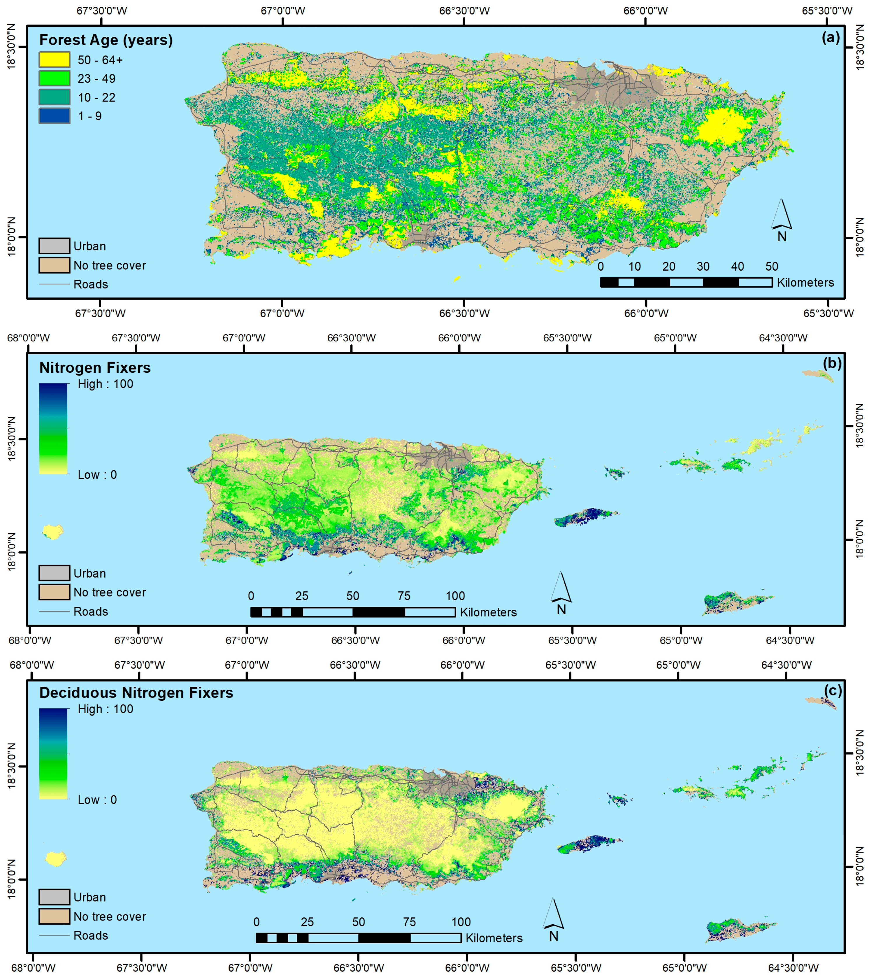
4.1. Forest Spatial Patterns Reflect Stand Age, Geoclimate, and Disturbance History

4.1.1. Biophysical, Socioeconomic, and Landscape Controls on Forest Recovery

Because the spatial pattern of stand age was apparent in the patterns of several of the mapped forest attributes, we briefly discuss here its drivers. In Puerto Rico and elsewhere, the biophysical, socioeconomic, and landscape variables that drive the spatial patterns of forest recovery are those that affect land accessibility, arability, market forces, seed dispersal, and microclimate, as well as spatial contagion related to these drivers [42,43]. The oldest forests are usually more remote, which in the study area means further from roads, cities, and coastlines and at higher elevations where slopes are steeper and which in Puerto Rico may be cloud-shrouded and have water-logged soils. Older forests also occur over rugged geology with fast-draining, nutrient-poor, or toxic soils (karst, serpentine) or in places that are less accessible or arable in other ways, such as being protected or being wetlands. These are the places where agriculture was abandoned the soonest or that may never have been cleared. Being less in demand for human uses, except perhaps watershed stabilization, many of these areas were among the first to be protected (Figure 3). In Puerto Rico and elsewhere, protected areas may have been designated where protection is the least inconvenient for humans [72,73]. Forests closer to cities and roads, on gentler slopes, and at lower elevations are increasingly younger. The earliest forests to be abandoned and recover are the last to have been cleared. Then, the next sites to be abandoned are closer to remaining or existing forest and receive more seed dispersal and have a cooler and more humid microclimate, enhancing forest recovery. This cycle of interacting socioeconomic and biophysical drivers, including landscape variables like spatial contagion, make distance to existing forest, or its usual complement, distance to pasture, the strongest predictors of the spatial patterns of forest regrowth and stand age [42,43,74]. The nearby forest can be secondary or old-growth forest.

Studies have found exceptions to these trends in other tropical countries. Farmers may clear less accessible land for agriculture where they find new opportunities for profit from agriculture or perceive that their best option for income or subsistence is unsanctioned forest clearing for agriculture in more remote areas, including in protected areas or other state-owned land [75,76]. As mentioned, protection also makes lands less accessible, and protected areas are not always in the least arable geoclimates. An example is the island of St. John, two-thirds of which was privately owned for some time and then became a National Park. Forest in the park is older compared with that on the other islands east of mainland Puerto Rico, even though it has geoclimates similar to other smaller islands in the study area.

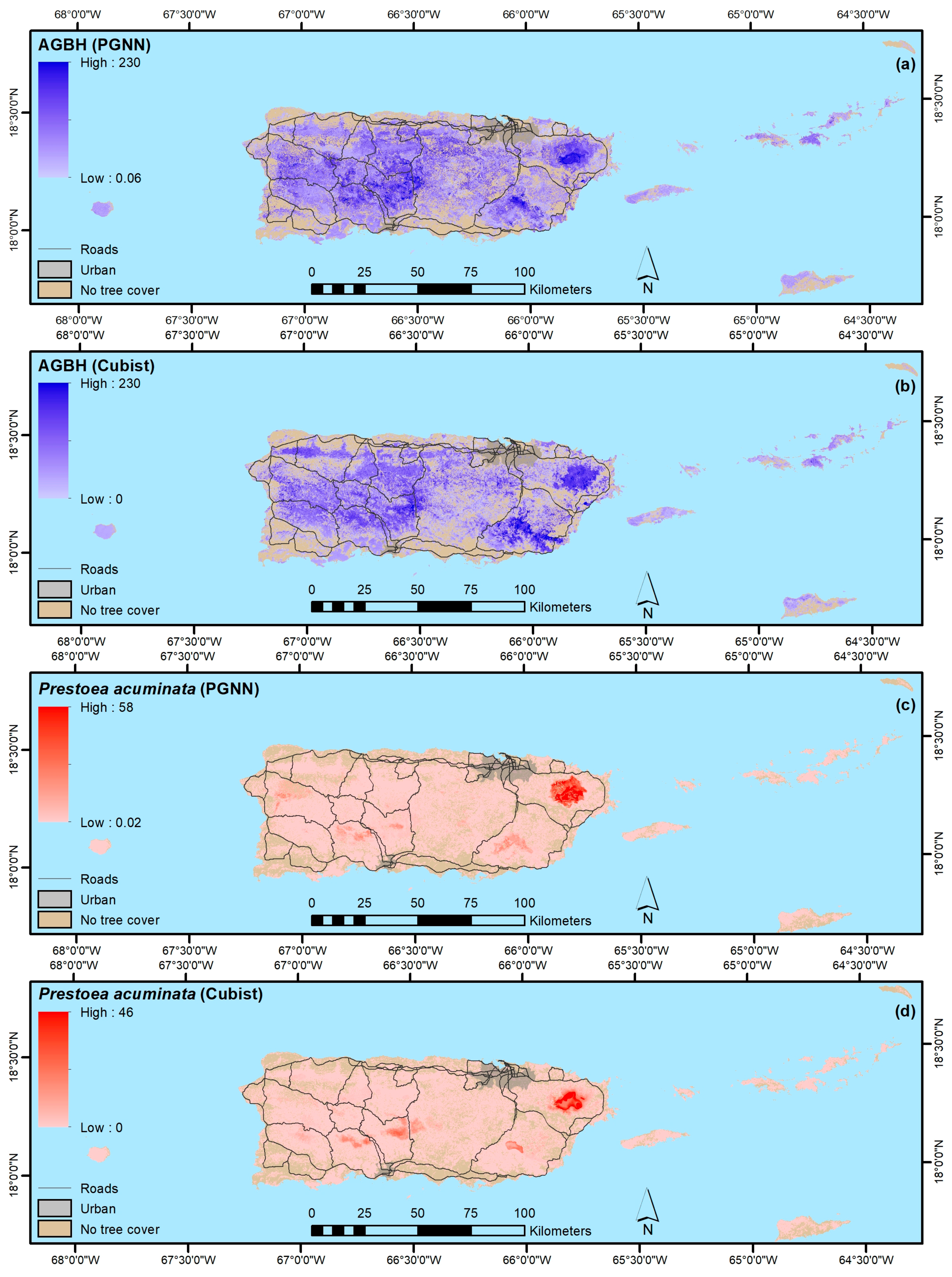
4.1.2. Forest Structure and Biomass

The maps of forest biomass (Figure 4), height, and basal area reflect the strong relationships between forest structure and (1) stand age and (2) geoclimate. Plot-level biomass averages across Puerto Rico by age class, geology, and climate (as gauged by leaf physiognomy) support this observation [43]. In plot-level studies, stand age has been the best predictor of young tropical forest biomass, height, or basal area [36,77,78,79] for a given geoclimate. If other landscape characteristics are the same, older forests have more biomass. Also apparent are the abovementioned biophysical and socioeconomic controls on forest regrowth spatial patterns. Younger forests are those closest to coastlines or the largest cities or roads, and they have less biomass (light blue to white shades in the biomass map). Forests at higher elevations or further from roads have more biomass.

Stand age is a critical component of forest carbon cycling as well. Net ecosystem productivity, for example, strongly correlates with age. Intermediate-aged forests are most productive, but old-growth forests can be huge carbon sinks [80], accumulating carbon for centuries. The rate of C accumulation in large trees increases with age, and clearing old-growth forest releases more carbon than can be accumulated by young forests [81,82].

Geoclimate is also important. Forest biomass differs by geologic substrate when averaged across age classes for a given climate zone. The forests with the most biomass are on volcanic or alluvial geologic substrates, which are fertile. Forest in karst zones has less biomass, being edaphically dry. Ultramafic, serpentine soils support the least forest biomass for a given climate, being edaphically dry plus nutrient poor and toxic. Geology likely influences forest biomass across the tropics, including in the Amazon basin [41]. As for climate, within the same geology and age class, humid forests (blue shades in the PET/P map in Figure 1) have more biomass than stands in drier places (white to brown shades in the PET/P map). Cloud forests on peaks, however, are stunted by water-logged soils, increased ultraviolet-B radiation, and high winds.

Disturbance history variables other than forest age affect tropical forest height and rates of biomass accumulation [36,79], but they are less obvious in these regional maps of forest structure. As well, the effects of finer-scaled topography on forest biomass were inconsistent in the maps. Topography likely influences forest biomass, however. In Panama moist forests, concave slopes have more biomass than convex ones [83]. Trees are visibly larger in valleys and concave slopes in dry and edaphically dry parts of the study area as well.

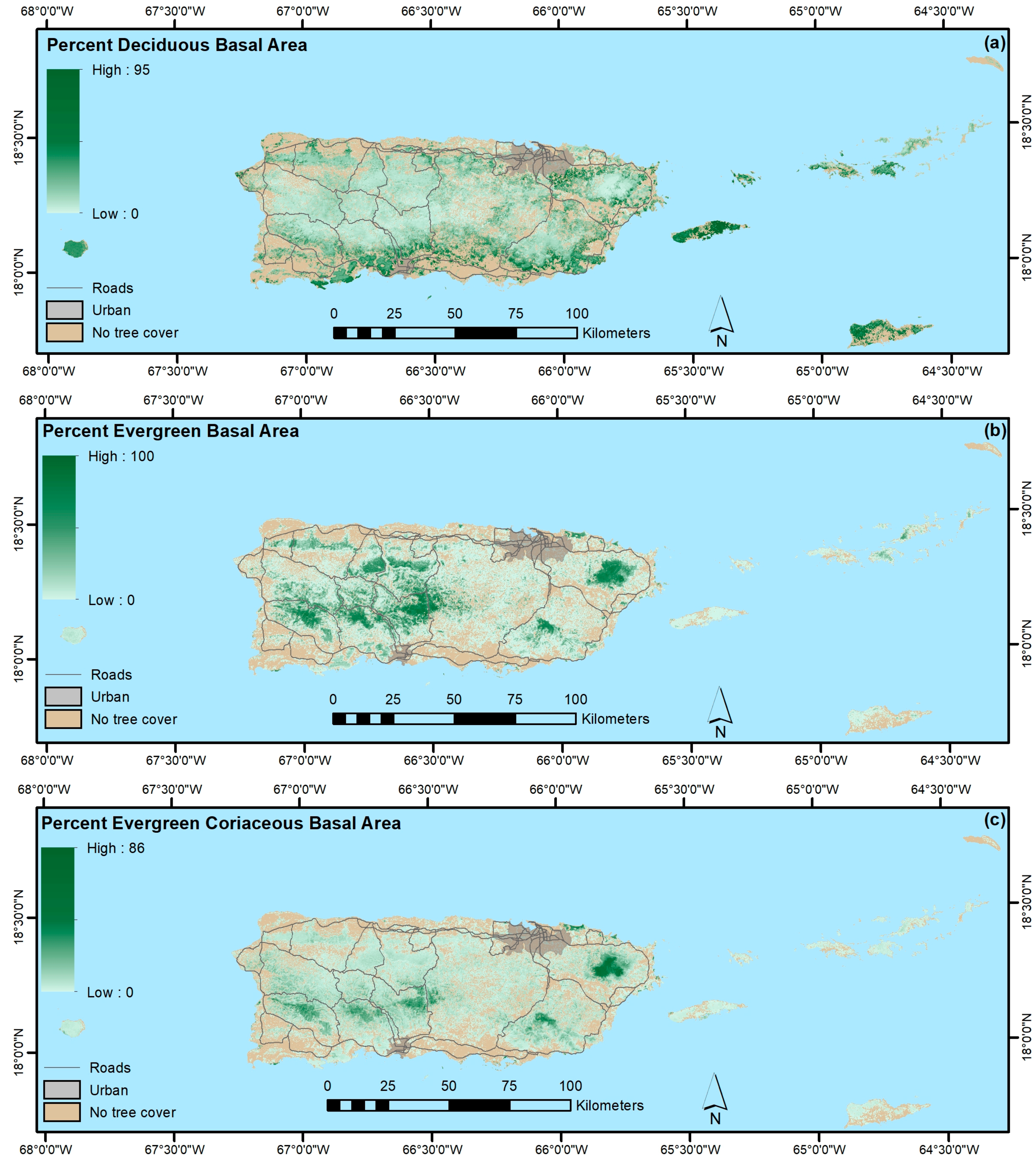
4.1.3. Forest Functional Groups

The effects of stand age and climate are also evident in the maps of relative basal areas of N-fixing and deciduous N-fixing tree species (Figure 5). These attributes are low (yellow in color) in the oldest forests and high in young forests (deep blue color), particularly so for dry forests (Figure 5a–c). Deciduous N-fixing relative basal areas are largest in young dry forests, but they are also large in the youngest forests in humid areas. Pioneer tree species are often N-fixers [84], and N-fixing trees have long been planted as part of land reclamation plans, including in tropical regions [85,86]. Even without planting, N-fixing tree species are common in tropical forest pioneer stands, and their prevalence declines with age [87,88,89]. This tendency applies to Puerto Rico, where younger forests across climates have larger relative basal areas of N-fixing species, many of them introduced [87]. Besides stand age, moisture availability affects the prevalence of N-fixing species. Tropical dry forests in general have more legumes compared with tropical humid forests [88,89]. For many legumes, the capacity to fix N and small leaflet sizes probably help them survive seasonal drought [89]. In addition, the larger N-fixing basal area appearing in Central Puerto Rico at higher elevations could also reflect the presence of N-fixing species in former shade coffee, including Inga laurina ((Sw.) Willd.) and Andira inermis ((W. Wright Kunth ex DC.), and N-fixing species planted for shade coffee, including Inga vera (Willd.) and Erythrina poeppigiana ((Walp.) O.F. Cook). In the Virgin Islands, the maps indicate that N-fixing species numbers and relative basal area are low in St. John, with its older forests. Other protected, older-forest areas in these islands show a similar pattern.

In the leaf phenology maps, relative basal areas of evergreen species are larger in more humid zones, while deciduous species have larger relative basal area in dry zones, as is typical of tropical forest landscapes (Figure 6a,b). Deciduous species, however, also have relatively more basal area in humid areas in younger forests, like those south and southeast of San Juan. The youngest tropical forests tend to be more deciduous in humid zones in Puerto Rico and elsewhere, probably because shorter leaf longevity protects against desiccation in the drier microclimate of young forest [70,90,91].

The maps of evergreen coriaceous species (Figure 6c) also show large relative basal areas on serpentine substrates (the westernmost dark green patches), in cloud forests (the remaining dark green patches at the highest elevations), and in mangrove forests (the small, dark green patches on coastlines). Hard leaves are typical in such places. Sclerophylly protects leaves in stressful environments [14,92,93].

Variables related to forest function, like nitrogen availability and leaf characteristics, are now critical to Earth system models. Until maps of such variables are available from more direct sources, maps like these can be used for running such models in a spatially explicit manner.

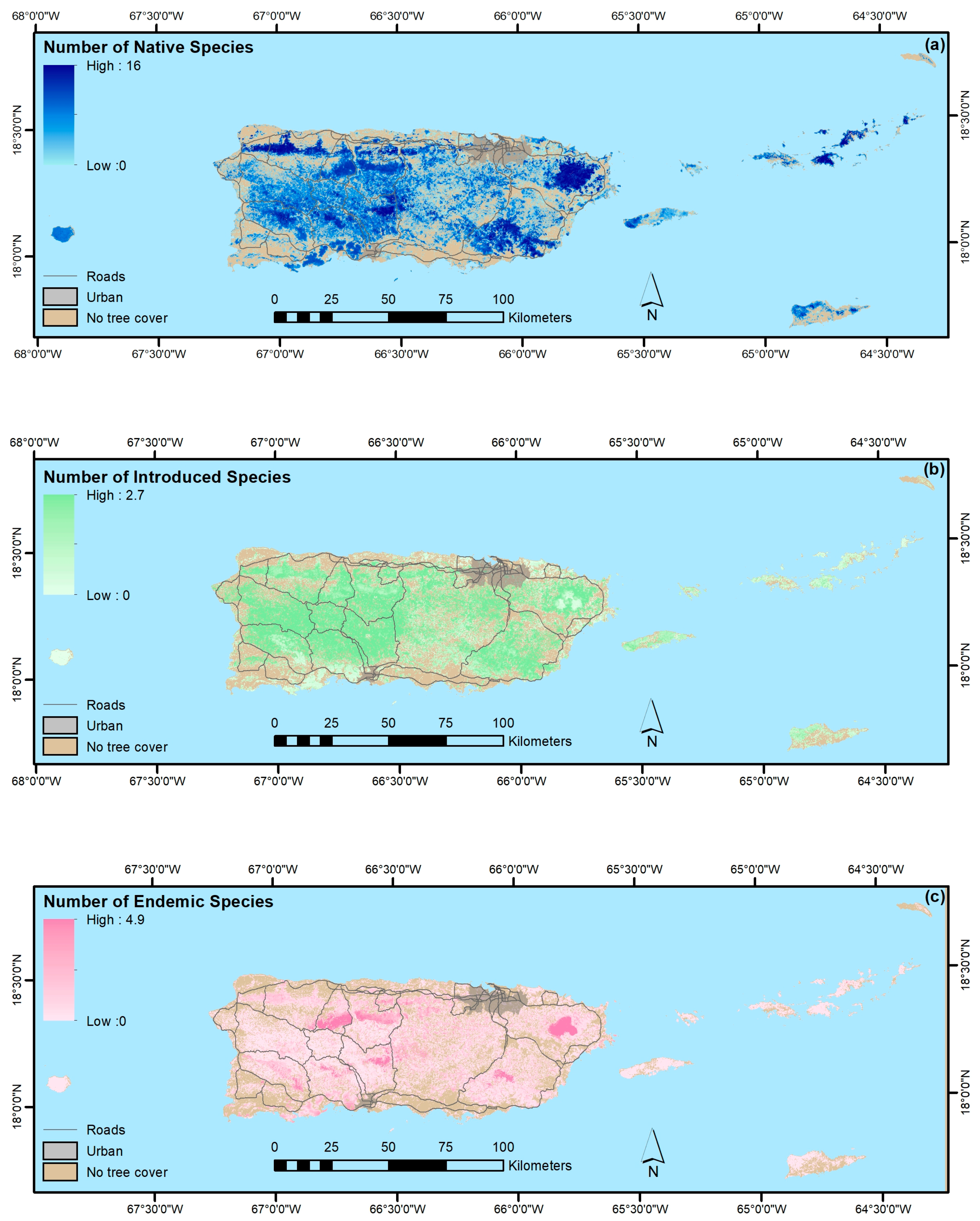
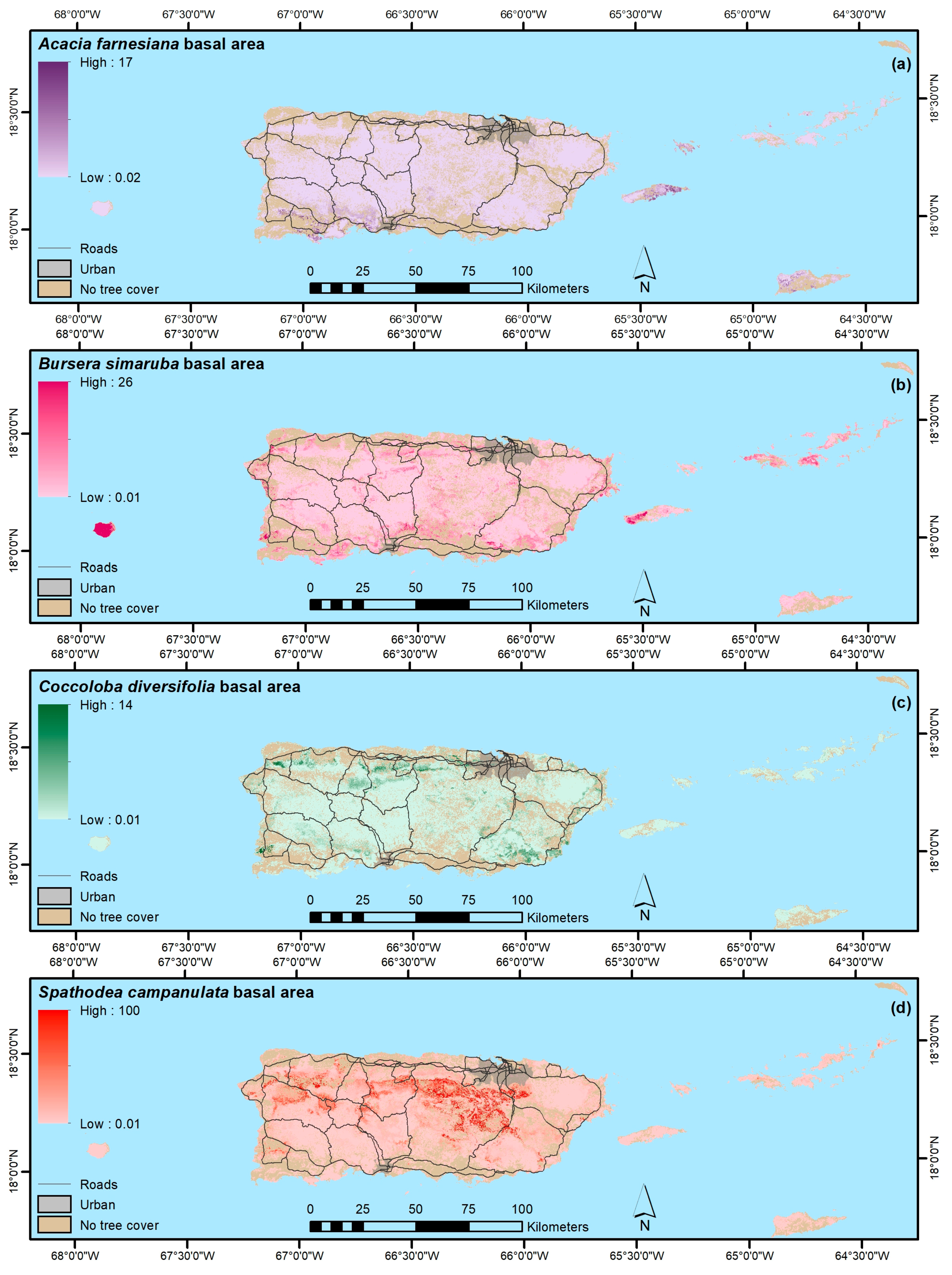
4.1.4. Native, Endemic, Introduced and Individual Species

Maps based on models that consider a majority of potentially important variables can help illustrate net impacts on forest species composition. Like forest structure and functional groups, spatial patterns of species counts, which are indicators of species richness and diversity, also follow the network of drivers that control forest age and include geoclimate and in some places land-use history. The maps of introduced species counts and relative basal areas (Figure 7 and Figure 8) show that introduced species are widespread across the study area and can often dominate stands. At the same time, they show that introduced species are uncommon in the abovementioned stressful environments: cloud forests and forests on serpentine substrate. These latter areas are among the least arable or accessible lands and, probably not coincidentally, are among the oldest forests that were made less accessible through relatively early protection. Introduced species are also less common in other of the longest-protected or inaccessible areas. Introduced species relative basal areas are increasingly larger as variables change in directions that that are most associated with forest clearing for agriculture: with decreasing elevation or ruggedness and decreasing distances to cities, and on volcanic, alluvial, or flat limestone substrates.

Plot-level studies encompassing the entire study region, all of Puerto Rico, in subregions of Puerto Rico, and elsewhere in the Caribbean [32,78,94,95,96,97,98,99,100], confirm that stands dominated by introduced species are widespread in the Caribbean islands. Disturbance type, including past or present land use, can strongly affect the species composition and diversity in Caribbean forests, including whether introduced species dominate forest regrowth [36,43,97,99,101,102]. Over time, however, a similar land use before abandonment [95] or seed sources in an area being limited to nearby secondary forest [103] can make climate [95] or time since abandonment [103] the drivers that most strongly impact species composition. In addition, native species seedlings can thrive in the understory of stands dominated by introduced species [104,105]. Plot-level studies also show that shade-tolerant introduced species, like Sysygium jambos ((L.) Alston), are are widespread in Puerto Rico, can dominate stands there, and can occur in older forests. Although it can persist for decades [78,102,106], it now appears to be susceptible to another introduced species, guava rust (Puccinia psidii Winter), which is relatively new to Puerto Rico [107]. Finally, introduced, fire-tolerant grasses in dry and dry-moist areas can dominate land for decades. The introduced Leucaena leucocephala ((Lam.) de Wit) can regenerate in these areas through its fast growth, partly suppressing these grasses while in some places providing protective shade for native seedlings [100,108,109].

Native and endemic species counts are mapped as being largest where forests are older and there has been less or less recent disturbance from land use. Puerto-Rico-wide plot-level studies show that species richness increases with basal area, stand age, proximity to the largest forest patches (which often encompass the oldest forests), and being on limestone or serpentine substrate, and that abandoned pasture is less diverse than recent shade coffee [43,97]. Smaller-scale studies in Puerto Rico and elsewhere in the tropics show that species richness increases with stand age or basal area [77,78,102] and proximity to old forest patches [110,111].

Endemic species counts and relative basal area are concentrated at the highest elevations, where cloud forests occur, and on serpentine and karst substrates. Larger endemic species counts and relative basal areas were mapped where the largest old forest patches occurred within these areas. Plots in Northeastern Puerto Rico also found more endemic species in the cloud forests there [112]. Endemic species often evolve in these environments, including in Puerto Rico, as they can be stressful and isolated [14,113,114,115,116].

For individual species with higher mapping model correlation coefficients between observed and predicted values, spatial patterns mapped with PGNN were as expected from field observation or published descriptions. Examples in Figure 9 include an introduced species found in young or frequently disturbed dry forests (Figure 9a); a common native species found in dry and edaphically dry places (Figure 9b); a native species typical of humid karst areas (Figure 9c); and the most common species in Puerto Rico, which is an introduced species (Figure 9d).

4.1.5. Implications for Sustainable Development Goal Indicators

The UN SDGs address terrestrial and freshwater ecosystems and their biodiversity and sustainable management in SDG 15 [117]. Many of its quantitative indicators are measures of national legislation or regulation. Examples are indicators (I) quantifying protected areas by ecosystem type (I 15.1.2), areas under sustainable forest management (I 15.2.1), protected areas important for mountain biodiversity (I 15.4.1), and legislation on invasive alien species (I 15.8.1). The five subindicators of progress towards sustainable forest management (I 15.2.1) include: (1) net rate of change in forest area, (2) change in aboveground biomass stocks in forest and forest area or area proportion under (3) legal protection, (4) a long-term management plan, or (5) a certified management plan.

Several of the maps we present are relevant to these SDG indicators and could help communicate to decision makers and the public the concepts or effects of these SDGs. They indicate important sites for biodiversity conservation (SDG Indicator 15.1.2), showing forest with high concentrations of native and endemic tree species. These areas have unique climate (cloud forests, also addressing SDG Indicator 15.4.1, important sites for mountain biodiversity) or geological substrate (serpentine and karst). In the case of Puerto Rico, a large portion of these areas is protected. Despite this protection advantage, some ecological zones and the ranges of many species remain poorly represented by protected areas, implying that more protection is needed there [70,72]. The maps also depict forest biomass (I 15.2.1) and introduced species spatial patterns (I 15.8.1).

We note that many of the introduced species are pioneer species that are shade-intolerant and consequently expected to decline with stand age as canopies close during forest succession. They are also mostly deciduous. A drawback of the maps is that the model of the common introduced tree species S. jambos was poor. It is an evergreen species, and because it is shade tolerant, it has more potential to be invasive than the other most common introduced species (though, as mentioned, it is being impacted by guava rust). It has one of the lowest correlation coefficients between observed and predicted basal areas. In other words, the predictor variables that we used may only be effective for mapping introduced species that are common in young or disturbed forests or that are deciduous. Other data are needed to map introduced species that are evergreen and can colonize older evergreen forest stands.

In addition, concern over the effects of overfertilization of terrestrial ecosystems with macronutrients like nitrogen [118] have led scientists to call for SDG indicators related to atmospheric nitrogen deposition [119]. Although it is a macronutrient, adding nitrogen to secondary tropical forests is thought to enhance tropical forest growth, but it can also inhibit growth [120,121]. In addition, increasing the basal area of N-fixing trees, including exotic species or species other than legumes, increases nitrogen levels in leaf litter, forest floor organic matter, or soils, and soils of secondary tropical forests release more NOx to the atmosphere [28,87,104,109,122], and NOx’s are potent greenhouse gases. The maps here illustrate where N-fixing species are most abundant.

4.2. Modeling Forest Characteristics vs. Modeling Individual Tree Species

As mentioned, the Cubist models of forest structure, species counts, and relative basal areas of functional groups and species origin usually had larger correlations between observed and predicted values than did PGNN models, even when test data included nonforest. A previous comparison of plot-level biomass values [123] similarly found that Cubist model outputs more closely matched observed values than GNN. The likely source of this tendency is that, here, the PGNN model is based on relative basal areas of all tree species rather than the particular structural, functional, or species origin variable being modeled. Even though species composition is related to structural and functional forest attributes, our results suggest that training individual models directly with these latter variables could better optimizes models. This approach could be tested for PGNN and GNN.

Although basing models on the relationships between the basal areas of all species and environmental gradients may be a disadvantage for modeling structural, functional, and diversity summaries, it apparently gives GNN and PGNN an advantage when mapping individual species distributions, as might be expected. Most tree species are associated with one or more communities of other tree species. Mapping tree species distributions with ordination axes improves maps of species that are rarely sampled, as previously observed [12,69], compared with models based only on such species occurrences. The ordination approach probably has the effect of increasing the number of observations of a species by virtue of that species’ association with other species in a dataset. A linear regression of the correlation coefficients of observed vs. predicted values for species-level models against the number of nonzero observations for each species explained no variability in the range of these coefficients for the PGNN approach but 20% of the range of correlation coefficients for the Cubist model results. This relationship suggests that Cubist results are more sensitive to the number of nonzero observations of species in the dataset than are PGNN results.

Species with highly predictable ranges, however, like the Sierra Palm, (Prestoea acuminata var. montana ((Willd.) H.E. Moore var. montana (Graham) A. Hend. & G. Galeano), were mapped well by both PGNN and Cubist (Figure 4), despite having few positive observations. It occurs only at higher elevations on mainland Puerto Rico in humid forest zones. Prior work in temperate forests also finds that species with “strong climate controls” or “limited range” were the most easily mapped ones [11]. Bursera simaruba ((L.) Sarg.) occurs on all islands. It had the most observations and the largest correlation coefficients between observed and predicted values. It, too, has a highly predictable range of occurring mainly in drier forests or in humid forests on the tops and sides of limestone hills. These coefficients were much smaller for Spathodea campanulata (P. Beauv.), the second most commonly observed species in the dataset. The most likely reason is that it is a widespread pioneer species. Besides a humid climate, which covers most of mainland Puerto Rico, the only thing it seems to need is sunlight [94,96,97,103]. Prior work also found widespread species more difficult to map [11].

5. Conclusions

From the mapping results, prior studies, and international sustainability goals, we conclude that:

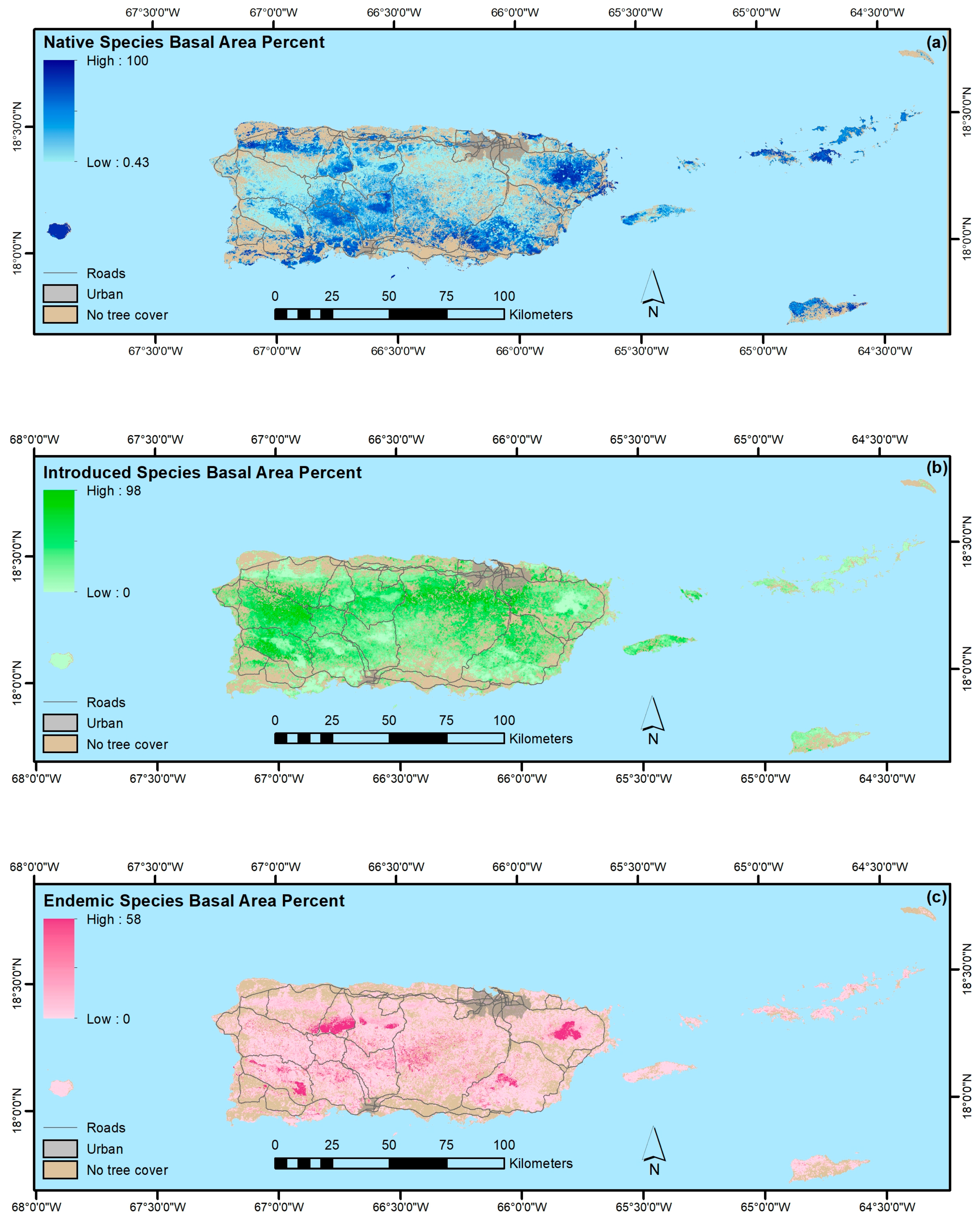
• The legacy of past large-scale clearing and subsequent forest recovery are clear when mapping current forest attributes in this tropical region. Introduced species are widespread across most of Puerto Rico and the Virgin Islands, and they often dominate stands. Moreover, introduced species are most prominent in younger forests. They are less common or rare, however, in the least-arable geoclimatic zones or more remote places.
• Native species counts are usually larger than counts of introduced species, and their relative basal areas tend to increase with stand age. Endemic species are concentrated in the oldest forests, which are in the least arable and most remote locations, including isolated extreme environments where endemic species often evolve, that were also, probably not coincidentally, protected early and in some places never cleared.
• Our mapping models explained a minority of the variance in forest attributes. Still, our results suggest that PGNN is better than regression tree models for mapping individual species and that, as in others’ work, the most common species are generally not the most accurately mapped ones. Instead, species with ranges limited by climate or other environmental factors are most easily mapped. Further, ordination in particular likely helps map species by virtue of their association with other species, which in effect increases the sample size for model training.
• In contrast, regression tree models appear to be better than ordination-based models for mapping other forest attributes, like forest biomass, functional groups, and species origin, at least when species basal areas are used to fit the ordination-based models.
• Several forest attributes addressed in UN SDGs have spatial patterns that reflect stand age, geoclimate, and aspects of disturbance history other than stand age since abandonment or last disturbance, like past disturbance type or intensity. Forest age, height, biomass, or disturbance-type history can now be mapped more accurately with long time series of globally available imagery [53,124,125,126,127,128]. Our results suggest that such maps, when combined with climate and lithology maps, would be useful for monitoring related to SDGs.

References

1. Achard, F.; Beuchle, R.; Mayaux, P.; Stibig, H.-J.; Bodart, C.; Brink, A.; Carboni, S.; Desclée, B.; Donnay, F.; Eva, H.D.; et al. Determination of tropical deforestation rates and related carbon losses from 1990 to 2010. Glob. Chang. Biol. 2014, 20, 2540–2554. [Google Scholar] [CrossRef] [PubMed] [Green Version]
2. Dirzo, R.; Raven, P.H. Global State of Biodiversity and Loss. Annu. Rev. Environ. Resour. 2003, 28, 137–167. [Google Scholar] [CrossRef]
3. Bradshaw, C.J.; Sodhi, N.S.; Brook, B.W. Tropical turmoil: A biodiversity tragedy in progress. Front. Ecol. Environ. 2009, 7, 79–87. [Google Scholar] [CrossRef]
4. Pimm, S.L.; Raven, P. Extinction by numbers. Nature 2000, 403, 843. [Google Scholar] [CrossRef] [PubMed]
5. Berenguer, E.; Ferreira, J.; Gardner, T.A.; Oliveira Cruz Aragão, L.E.; Barbosa De Camargo, P.; Cerri, C.E.; Durigan, M.; Oliveira, R.C.D.; Vieira, I.C.G.; Barlow, J. A large-scale field assessment of carbon stocks in human-modified tropical forests. Glob. Chang. Biol. 2014, 20, 3713–3726. [Google Scholar] [CrossRef] [PubMed] [Green Version]
6. Gardner, T.A.; Barlow, J.; Sodhi, N.S.; Peres, C.A. A multi-region assessment of tropical forest biodiversity in a human-modified world. Biol. Conserv. 2010, 143, 2293–2300. [Google Scholar] [CrossRef]
7. Gardner, T.A.; Barlow, J.; Chazdon, R.; Ewers, R.M.; Harvey, C.A.; Peres, C.A.; Sodhi, N.S. Prospects for tropical forest biodiversity in a human-modified world. Ecol. Lett. 2009, 12, 561–582. [Google Scholar] [CrossRef] [PubMed]
8. Gibson, L.; Lee, T.M.; Koh, L.P.; Brook, B.W.; Gardner, T.A.; Barlow, J.; Peres, C.A.; Bradshaw, C.J.A.; Laurance, W.F.; Lovejoy, T.E.; et al. Primary forests are irreplaceable for sustaining tropical biodiversity. Nature 2011, 478, 378. [Google Scholar] [CrossRef] [PubMed]
9. Barlow, J.; Gardner, T.A.; Araujo, I.S.; Ávila-Pires, T.C.; Bonaldo, A.B.; Costa, J.E.; Esposito, M.C.; Ferreira, L.V.; Hawes, J.; Hernandez, M.I.M.; et al. Quantifying the biodiversity value of tropical primary, secondary, and plantation forests. Proc. Natl. Acad. Sci. USA 2007, 104, 18555–18560. [Google Scholar] [CrossRef] [PubMed] [Green Version]
10. Rulequest. Data Mining with Cubist, Rulequest Research. 2018. Available online: https://www.rulequest.com/cubist-info.html (accessed on 31 October 2018).
11. Ohmann, J.L.; Gregory, M.J. Predictive mapping of forest composition and structure with direct gradient analysis and nearest-neighbor imputation in coastal Oregon, U.S.A. Can. J. For. Res. 2002, 32, 725–741. [Google Scholar] [CrossRef]
12. Wilson, B.T.; Lister, A.J.; Riemann, R.I. A nearest-neighbor imputation approach to mapping tree species over large areas using forest inventory plots and moderate resolution raster data. For. Ecol. Manag. 2012, 271, 182–198. [Google Scholar] [CrossRef]
13. Wilson, B.T.; Woodall, C.W.; Griffith, D.M. Imputing forest carbon stock estimates from inventory plots to a nationally continuous coverage. Carbon Balance Manag. 2013, 8, 1. [Google Scholar] [CrossRef] [PubMed]
14. Whittaker, R.H. The Ecology of Serpentine Soils. Ecology 1954, 35, 258–288. [Google Scholar] [CrossRef]
15. USDA Forest Service. Forest Service. Forest inventory and analysis national core field guide. In Field Data Collection Procedures for Phase 2 Plots; Version 6.11; U.S. Department of Agriculture Forest Service: Washington, DC, USA, 2014; Volume 1, p. 305. [Google Scholar]
16. Acevedo-Rodríguez, P. Flora of St. John, US Virgin Islands; New York Botanical Garden Bronx: New York, NY, USA, 1996. [Google Scholar]
17. Little, E.L.; Wadsworth, F.H. Common trees of Puerto Rico and the Virgin Islands, Vol 2; USDA Forest Service, Agriculture Handbook No. 449: Washington, DC, USA, 1974. [Google Scholar]
18. Little, E.L.; Woodbury, R.O.; Wadsworth, F.H. Trees of Puerto Rico and the Virgin Islands Vol 1; USDA Forest Service, Agriculture Handbook No. 249: Washington, DC, USA, 1964.
19. Liogier, A.H. Descriptive Flora of Puerto Rico and Adjacent Islands. Vol II: Leguminosae to Anacardiaceae; Editorial de la Universidad de Puerto Rico: Río Piedras, Puerto Rico, 1988. [Google Scholar]
20. Liogier, A.H. Descriptive Flora of Puerto Rico and Adjacent Islands. Vol. I: Casuarinaceae to Connaraceae; Editorial de la Universidad de Puerto Rico: Río Piedras, Puerto Rico, 1985. [Google Scholar]
21. Liogier, A.H. Descriptive Flora of Puerto Rico and Adjacent Islands. Vol. V: Acanthaceae to Compositae; Editorial de la Universidad de Puerto Rico: Río Piedras, Puerto Rico, 1997. [Google Scholar]
22. Liogier, A.H. Descriptive Flora of Puerto Rico and Adjacent Islands. Vol. III: Cyrillaceae to Myrtaceae; Editorial de la Universidad de Puerto Rico: Río Piedras, Puerto Rico, 1994. [Google Scholar]
23. Liogier, A.H.; Martorell, L.F. Flora of Puerto Rico and Adjacent Islands: A Systematic Synopsis; Editorial de la Universidad de Puerto Rico: Río Piedras, Puerto Rico, 2000. [Google Scholar]
24. Gibney, E. A Field Guide to Native Trees & Plants of East End, St. John, US Virgin Islands; Center for the Environment: St. John, U.S. Virgin Islands, USA, 2004; p. 86. [Google Scholar]
25. Scurlock, J.P. Native Trees and Shrubs of the Florida Keys: A Field Guide; Laurel Press: Pittsburg, PA, USA, 1987; p. 220. [Google Scholar]
26. Weaver, P.L.; Schwagerl, J.J. US Fish and Wildlife Service Refuges and Other Nearby Reserves in Southwestern Puerto Rico; International Institute of Tropical Forestry, USDA Forest Service: Río Piedras, Puerto Rico, 2009.
27. Kew. Seed Information Database (SID). Available online: http://data.kew.org/sid/ (accessed on 1 January 2011).
28. Erickson, H.E.; Helmer, E.H.; Brandeis, T.J.; Lugo, A.E. Controls on fallen leaf chemistry and forest floor element masses in native and novel forests across a tropical island. Ecosphere 2014, 5, art48. [Google Scholar] [CrossRef] [Green Version]
29. Gond, V.; Freycon, V.; Molino, J.-F.; Brunaux, O.; Ingrassia, F.; Joubert, P.; Pekel, J.-F.; Prévost, M.-F.; Thierron, V.; Trombe, P.-J.; et al. Broad-scale spatial pattern of forest landscape types in the Guiana Shield. Int. J. Appl. Earth Obs. Geoinf. 2011, 13, 357–367. [Google Scholar] [CrossRef]
30. Gwenzi, D.; Helmer, E.; Zhu, X.; Lefsky, M.; Marcano-Vega, H. Predictions of Tropical Forest Biomass and Biomass Growth Based on Stand Height or Canopy Area Are Improved by Landsat-Scale Phenology across Puerto Rico and the U.S. Virgin Islands. Remote Sens. 2017, 9, 123. [Google Scholar] [CrossRef]
31. Helmer, E.; Goodwin, N.R.; Gond, V.; Souza, C.M., Jr.; Asner, G.P. Characterizing tropical forests with multispectral imagery. Land Resour. 2015, 2, 367–396. [Google Scholar]
32. Helmer, E.H.; Ruzycki, T.S.; Benner, J.; Voggesser, S.M.; Scobie, B.P.; Park, C.; Fanning, D.W.; Ramnarine, S. Detailed maps of tropical forest types are within reach: Forest tree communities for Trinidad and Tobago mapped with multiseason Landsat and multiseason fine-resolution imagery. For. Ecol. Manag. 2012, 279, 147–166. [Google Scholar] [CrossRef]
33. Helmer, E.H.; Ruefenacht, B. Cloud-Free Satellite Image Mosaics with Regression Trees and Histogram Matching. Photogramm. Eng. Remote Sens. 2005, 71, 1079–1089. [Google Scholar] [CrossRef]
34. Helmer, E.H.; Ruefenacht, B. A comparison of radiometric normalization methods when filling cloud gaps in Landsat imagery. Can. J. Remote Sens. 2007, 33, 325–340. [Google Scholar] [CrossRef]
35. Helmer, E.H.; Brown, S.; Cohen, W.B. Mapping montane tropical forest successional stage and land use with multi-date Landsat imagery. Int. J. Remote Sens. 2000, 21, 2163–2183. [Google Scholar] [CrossRef]
36. Helmer, E.H.; Ruzycki, T.S.; Wunderle, J.M.; Vogesser, S.; Ruefenacht, B.; Kwit, C.; Brandeis, T.J.; Ewert, D.N. Mapping tropical dry forest height, foliage height profiles and disturbance type and age with a time series of cloud-cleared Landsat and ALI image mosaics to characterize avian habitat. Remote Sens. Environ. 2010, 114, 2457–2473. [Google Scholar] [CrossRef]
37. Kennaway, T.; Helmer, E.H. The Forest Types and Ages Cleared for Land Development in Puerto Rico. GISci. Remote Sens. 2007, 44, 356–382. [Google Scholar] [CrossRef]
38. Kennaway, T.A.; Helmer, E.H.; Lefsky, M.A.; Brandeis, T.J.; Sherrill, K.R. Mapping land cover and estimating forest structure using satellite imagery and coarse resolution lidar in the Virgin Islands. J. Appl. Remote Sens. 2008, 2, 023551. [Google Scholar]
39. Daly, C.; Helmer, E.H.; Quiñones, M. Mapping the climate of Puerto Rico, Vieques and Culebra. Int. J. Climatol. 2003, 23, 1359–1381. [Google Scholar] [CrossRef] [Green Version]
40. Asner, G.P.; Mascaro, J.; Anderson, C.; Knapp, D.E.; Martin, R.E.; Kennedy-Bowdoin, T.; van Breugel, M.; Davies, S.; Hall, J.S.; Muller-Landau, H.C.; et al. High-fidelity national carbon mapping for resource management and REDD+. Carbon Balance Manag. 2013, 8, 7. [Google Scholar] [CrossRef] [PubMed] [Green Version]
41. Asner, G.P.; Powell, G.V.N.; Mascaro, J.; Knapp, D.E.; Clark, J.K.; Jacobson, J.; Kennedy-Bowdoin, T.; Balaji, A.; Paez-Acosta, G.; Victoria, E.; et al. High-resolution forest carbon stocks and emissions in the Amazon. Proc. Natl. Acad. Sci. USA 2010, 107, 16738–16742. [Google Scholar] [CrossRef] [PubMed] [Green Version]
42. Helmer, E.H. The Landscape Ecology of Tropical Secondary Forest in Montane Costa Rica. Ecosystems 2000, 3, 98–114. [Google Scholar] [CrossRef]
43. Helmer, E.H.; Brandeis, T.J.; Lugo, A.E.; Kennaway, T. Factors influencing spatial pattern in tropical forest clearance and stand age: Implications for carbon storage and species diversity. J. Geophys. Res. Biogeosci. 2008, 113. [Google Scholar] [CrossRef] [Green Version]
44. Huete, A.; Justice, C.; Van Leeuwen, W. MODIS Vegetation Index (MOD13) Algorithm Theoretical Basis Document; University of Arizona: Tucson, AZ, USA, 1999; p. 213. [Google Scholar]
45. Krushensky, R. Generalized geology map of Puerto Rico; US Geological Survey: San Juan, Puerto Rico, 1995.
46. Garrison, L.E.; Martin, R.; Berryhill, H.; Buell, M.; Ensminger, H.; Perry, R. Preliminary Tectonic Map of the Eastern Greater Antilles Region; U.S. Department of the Interior—Geological Survey: Washington, DC, USA, 1972.
47. Slater, J.A.; Garvey, G.; Johnston, C.; Haase, J.; Heady, B.; Kroenung, G.; Little, J. The SRTM data “finishing” process and products. Photogramm. Eng. Remote Sens. 2006, 72, 237–247. [Google Scholar] [CrossRef]
48. Homer, C.; Huang, C.; Yang, L.; Wylie, B.; Coan, M. Development of a 2001 National Land-Cover Database for the United States. Photogramm. Eng. Remote Sens. 2004, 70, 829–840. [Google Scholar] [CrossRef]
49. Quinlan, J.R. Improved use of continuous attributes in C4.5. J. Artif. Intell. Res. 1996, 4, 77–90. [Google Scholar] [CrossRef]
50. Walton, J.T. Subpixel Urban Land Cover Estimation. Photogramm. Eng. Remote Sens. 2008, 74, 1213–1222. [Google Scholar] [CrossRef]
51. Blackard, J.A.; Finco, M.V.; Helmer, E.H.; Holden, G.R.; Hoppus, M.L.; Jacobs, D.M.; Lister, A.J.; Moisen, G.G.; Nelson, M.D.; Riemann, R.; et al. Mapping U.S. forest biomass using nationwide forest inventory data and moderate resolution information. Remote Sens. Environ. 2008, 112, 1658–1677. [Google Scholar] [CrossRef]
52. Lefsky, M.A. A global forest canopy height map from the Moderate Resolution Imaging Spectroradiometer and the Geoscience Laser Altimeter System. Geophys. Res. Lett. 2010, 37. [Google Scholar] [CrossRef] [Green Version]
53. Li, A.; Huang, C.; Sun, G.; Shi, H.; Toney, C.; Zhu, Z.; Rollins, M.G.; Goward, S.N.; Masek, J.G. Modeling the height of young forests regenerating from recent disturbances in Mississippi using Landsat and ICESat data. Remote Sens. Environ. 2011, 115, 1837–1849. [Google Scholar] [CrossRef]
54. Rudiyanto; Budiman, M.; Budi Indra, S.; Chusnul, A.; Saptomo, S.K.; Chadirin, Y. Digital mapping for cost-effective and accurate prediction of the depth and carbon stocks in Indonesian peatlands. Geoderma 2016, 272, 20–31. [Google Scholar] [CrossRef]
55. Breiman, L. Random Forests. Mach. Learn. 2001, 45, 5–32. [Google Scholar] [CrossRef] [Green Version]
56. Aertsen, W.; Kint, V.; van Orshoven, J.; Özkan, K.; Muys, B. Comparison and ranking of different modelling techniques for prediction of site index in Mediterranean mountain forests. Ecol. Model. 2010, 221, 1119–1130. [Google Scholar] [CrossRef]
57. Colditz, R. An Evaluation of Different Training Sample Allocation Schemes for Discrete and Continuous Land Cover Classification Using Decision Tree-Based Algorithms. Remote Sens. 2015, 7, 9655. [Google Scholar] [CrossRef]
58. Hudak, A.T.; Crookston, N.L.; Evans, J.S.; Hall, D.E.; Falkowski, M.J. Nearest neighbor imputation of species-level, plot-scale forest structure attributes from LiDAR data. Remote Sens. Environ. 2008, 112, 2232–2245. [Google Scholar] [CrossRef]
59. Ter Braak, C.J. The analysis of vegetation-environment relationships by canonical correspondence analysis. Vegetatio 1987, 69, 69–77. [Google Scholar] [CrossRef] [Green Version]
60. Ohmann, J.L.; Gregory, M.J.; Roberts, H.M.; Cohen, W.B.; Kennedy, R.E.; Yang, Z. Mapping change of older forest with nearest-neighbor imputation and Landsat time-series. For. Ecol. Manag. 2012, 272, 13–25. [Google Scholar] [CrossRef]
61. Pierce, K.B.; Ohmann, J.L.; Wimberly, M.C.; Gregory, M.J.; Fried, J.S. Mapping wildland fuels and forest structure for land management: A comparison of nearest neighbor imputation and other methods. Can. J. For. Res. 2009, 39, 1901–1916. [Google Scholar] [CrossRef]
62. Steinberg, D.; Colla, P. CART: Classification and regression trees. Top Ten Algorithms Data Min. 2009, 9, 179. [Google Scholar]
63. Ruefenacht, B.; Finco, M.V.; Nelson, M.D.; Czaplewski, R.; Helmer, E.H.; Blackard, J.A.; Holden, G.R.; Lister, A.J.; Salajanu, D.; Weyermann, D.; et al. Conterminuous US and Alaska forest type mapping using forest inventory and analysis data. Photogramm. Eng. Remote Sens. 2008, 74, 1379–1388. [Google Scholar] [CrossRef]
64. Dray, S.; Dufour, A.-B. The ade4 Package: Implementing the Duality Diagram for Ecologists. J. Stat. Softw. 2007, 22, 20. [Google Scholar] [CrossRef]
65. Li, M.; Im, J.; Quackenbush, L.J.; Liu, T. Forest Biomass and Carbon Stock Quantification Using Airborne LiDAR Data: A Case Study Over Huntington Wildlife Forest in the Adirondack Park. IEEE J. Sel. Top. Appl. Earth Observ. Remote Sens. 2014, 7, 3143–3156. [Google Scholar] [CrossRef]
66. Ohmann, J.L.; Gregory, M.J.; Spies, T.A. Influence of environment, disturbance, and ownership on forest vegetation of coastal Oregon. Ecol. Appl. 2007, 17, 18–33. [Google Scholar] [CrossRef]
67. Reese, H.; Nilsson, M.; Pahlén, T.G.; Hagner, O.; Joyce, S.; Tingelöf, U.; Egberth, M.; Olsson, H. Countrywide Estimates of Forest Variables Using Satellite Data and Field Data from the National Forest Inventory. AMBIO 2003, 32, 542–548. [Google Scholar] [CrossRef] [PubMed]
68. Sales, M.H.; Souza, C.M.; Kyriakidis, P.C.; Roberts, D.A.; Vidal, E. Improving spatial distribution estimation of forest biomass with geostatistics: A case study for Rondônia, Brazil. Ecol. Model. 2007, 205, 221–230. [Google Scholar] [CrossRef]
69. Elith, J.; Graham, C.H.; Anderson, R.P.; Dudík, M.; Ferrier, S.; Guisan, A.; Hijmans, R.J.; Huettmann, F.; Leathwick, J.R.; Lehmann, A. Novel methods improve prediction of species' distributions from occurrence data. Ecography 2006, 29, 129–151. [Google Scholar] [CrossRef]
70. Castro-Prieto, J.; Quiñones, M.; Gould, W. Characterization of the Network of Protected Areas in Puerto Rico. Caribb. Nat. 2016, 29, 1–16. [Google Scholar]
71. Gould, W.A.; Quinones, M.; Solorzano, M.; Alcobas, W.; Alarcon, C. Protected Natural Areas of Puerto Rico. 1:240,000, Res. Map IITF-RMAP-02; U.S. Department of Agriculture, Forest Service, International Institute of Tropical Forestry: Rio Piedras, Puerto Rico, 2011.
72. Helmer, E.H. Forest conservation and land development in Puerto Rico. Landsc. Ecol. 2004, 19, 29–40. [Google Scholar] [CrossRef]
73. Venter, O.; Magrach, A.; Outram, N.; Klein, C.J.; Possingham, H.P.; Di Marco, M.; Watson, J.E.M. Bias in protected-area location and its effects on long-term aspirations of biodiversity conventions. Conserv. Biol. 2018, 32, 127–134. [Google Scholar] [CrossRef] [PubMed]
74. Etter, A.; McAlpine, C.; Pullar, D.; Possingham, H. Modeling the age of tropical moist forest fragments in heavily-cleared lowland landscapes of Colombia. For. Ecol. Manag. 2005, 208, 249–260. [Google Scholar] [CrossRef]
75. Newman, M.E.; McLaren, K.P.; Wilson, B.S. Long-term socio-economic and spatial pattern drivers of land cover change in a Caribbean tropical moist forest, the Cockpit Country, Jamaica. Agric. Ecosyst. Environ. 2014, 186, 185–200. [Google Scholar] [CrossRef]
76. Nagendra, H.; Southworth, J.; Tucker, C. Accessibility as a determinant of landscape transformation in western Honduras: Linking pattern and process. Landsc. Ecol. 2003, 18, 141–158. [Google Scholar] [CrossRef]
77. Aide, T.M.; Zimmerman, J.K.; Pascarella, J.B.; Rivera, L.; Marcano-Vega, H. Forest Regeneration in a Chronosequence of Tropical Abandoned Pastures: Implications for Restoration Ecology. Restor. Ecol. 2000, 8, 328–338. [Google Scholar] [CrossRef]
78. Aide, T.M.; Zimmerman, J.K.; Rosario, M.; Marcano, H. Forest recovery in abandoned cattle pastures along an elevational gradient in northeastern Puerto Rico. Biotropica 1996, 28, 537–548. [Google Scholar] [CrossRef]
79. Zarin, D.J.; Davidson, E.A.; Brondizio, E.; Vieira, I.C.; Sá, T.; Feldpausch, T.; Schuur, E.A.; Mesquita, R.; Moran, E.; Delamonica, P.; et al. Legacy of fire slows carbon accumulation in Amazonian forest regrowth. Front. Ecol. Environ. 2005, 3, 365–369. [Google Scholar] [CrossRef] [Green Version]
80. Pregitzer, K.S.; Euskirchen, E.S. Carbon cycling and storage in world forests: Biome patterns related to forest age. Glob. Chang. Biol. 2004, 10, 2052–2077. [Google Scholar] [CrossRef]
81. Luyssaert, S.; Schulze, E.D.; Börner, A.; Knohl, A.; Hessenmöller, D.; Law, B.E.; Ciais, P.; Grace, J. Old-growth forests as global carbon sinks. Nature 2008, 455, 213. [Google Scholar] [CrossRef] [PubMed]
82. Stephenson, N.L.; Das, A.J.; Condit, R.; Russo, S.E.; Baker, P.J.; Beckman, N.G.; Coomes, D.A.; Lines, E.R.; Morris, W.K.; Rüger, N.; et al. Rate of tree carbon accumulation increases continuously with tree size. Nature 2014, 507, 90. [Google Scholar] [CrossRef] [PubMed]
83. Detto, M.; Muller-Landau, H.C.; Mascaro, J.; Asner, G.P. Hydrological Networks and Associated Topographic Variation as Templates for the Spatial Organization of Tropical Forest Vegetation. PLoS ONE 2013, 8, e76296. [Google Scholar] [CrossRef] [PubMed]
84. Finegan, B. Forest succession. Nature 1984, 312, 109. [Google Scholar] [CrossRef]
85. Chaer, G.M.; Resende, A.S.; Campello, E.F.C.; de Faria, S.M.; Boddey, R.M. Nitrogen-fixing legume tree species for the reclamation of severely degraded lands in Brazil. Tree Physiol. 2011, 31, 139–149. [Google Scholar] [CrossRef] [PubMed] [Green Version]
86. Franco, A.A.; De Faria, S.M. The contribution of N2-fixing tree legumes to land reclamation and sustainability in the tropics. Soil Biol. Biochem. 1997, 29, 897–903. [Google Scholar] [CrossRef]
87. Erickson, H.; Davidson, E.A.; Keller, M. Former land-use and tree species affect nitrogen oxide emissions from a tropical dry forest. Oecologia 2002, 130, 297–308. [Google Scholar] [CrossRef] [PubMed]
88. Gei, M.; Rozendaal, D.M.A.; Poorter, L.; Bongers, F.; Sprent, J.I.; Garner, M.D.; Aide, T.M.; Andrade, J.L.; Balvanera, P.; Becknell, J.M.; et al. Legume abundance along successional and rainfall gradients in Neotropical forests. Nat. Ecol. Evol. 2018. [Google Scholar] [CrossRef] [PubMed]
89. Powers, J.S.; Marín-Spiotta, E. Ecosystem Processes and Biogeochemical Cycles in Secondary Tropical Forest Succession. Annu. Rev. Ecol. Evol. Syst. 2017, 48, 497–519. [Google Scholar] [CrossRef]
90. Eamus, D. Ecophysiological traits of deciduous and evergreen woody species in the seasonally dry tropics. Trends Ecol. Evol. 1999, 14, 11–16. [Google Scholar] [CrossRef] [Green Version]
91. Jin, Y.; Russo, S.E.; Yu, M. Effects of light and topography on regeneration and coexistence of evergreen and deciduous tree species in a Chinese subtropical forest. J. Ecol. 2018, 106, 1634–1645. [Google Scholar] [CrossRef]
92. Leigh, E.G., Jr. Structure and climate in tropical rain forest. Annu. Rev. Ecol. Syst. 1975, 6, 67–86. [Google Scholar] [CrossRef]
93. Read, J.; Sanson, G.D.; Garine-Wichatitsky, M.; Jaffré, T. Sclerophylly in two contrasting tropical environments: Low nutrients vs. low rainfall. Am. J. Bot. 2006, 93, 1601–1614. [Google Scholar] [CrossRef] [PubMed]
94. Abelleira Martínez, O.J. Invasion by native tree species prevents biotic homogenization in novel forests of Puerto Rico. Plant Ecol. 2010, 211, 49–64. [Google Scholar] [CrossRef]
95. Brandeis, T.J.; Helmer, E.H.; Marcano-Vega, H.; Lugo, A.E. Climate shapes the novel plant communities that form after deforestation in Puerto Rico and the U.S. Virgin Islands. For. Ecol. Manag. 2009, 258, 1704–1718. [Google Scholar] [CrossRef]
96. Chinea, J.D. Tropical forest succession on abandoned farms in the Humacao Municipality of eastern Puerto Rico. For. Ecol. Manag. 2002, 167, 195–207. [Google Scholar] [CrossRef]
97. Chinea, J.D.; Helmer, E.H. Diversity and composition of tropical secondary forests recovering from large-scale clearing: Results from the 1990 inventory in Puerto Rico. For. Ecol. Manag. 2003, 180, 227–240. [Google Scholar] [CrossRef]
98. Helmer, E.H.; Kennaway, T.A.; Pedreros, D.H.; Clark, M.L.; Marcano-Vega, H.; Tieszen, L.L.; Ruzycki, T.R.; Schill, S.R.; Sean Carrington, C.M. Land Cover and Forest Formation Distributions for St. Kitts, Nevis, St. Eustatius, Grenada and Barbados from Decision Tree Classification of Cloud-Cleared Satellite Imagery. Caribbean J. Sci. 2008, 44, 175–198. [Google Scholar] [CrossRef]
99. Rivera, L.W.; Aide, T.M. Forest recovery in the karst region of Puerto Rico. For. Ecol. Manag. 1998, 108, 63–75. [Google Scholar] [CrossRef]
100. Wolfe, B.T.; Van Bloem, S.J. Subtropical dry forest regeneration in grass-invaded areas of Puerto Rico: Understanding why Leucaena leucocephala dominates and native species fail. For. Ecol. Manag. 2012, 267, 253–261. [Google Scholar] [CrossRef]
101. Larkin, C.C.; Kwit, C.; Wunderle, J.M.; Helmer, E.H.; Stevens, M.H.H.; Roberts, M.T.K.; Ewert, D.N. Disturbance Type and Plant Successional Communities in Bahamian Dry Forests. Biotropica 2012, 44, 10–18. [Google Scholar] [CrossRef]
102. Pascarella, J.B.; Aide, T.M.; Serrano, M.I.; Zimmerman, J.K. Land-Use History and Forest Regeneration in the Cayey Mountains, Puerto Rico. Ecosystems 2000, 3, 217–228. [Google Scholar] [CrossRef]
103. Marcano-Vega, H.; Mitchell Aide, T.; Báez, D. Forest regeneration in abandoned coffee plantations and pastures in the Cordillera Central of Puerto Rico. Plant Ecol. 2002, 161, 75–87. [Google Scholar] [CrossRef]
104. Parrotta, J.A. The role of plantation forests in rehabilitating degraded tropical ecosystems. Agric. Ecosyst. Environ. 1992, 41, 115–133. [Google Scholar] [CrossRef]
105. Parrotta, J.A.; Turnbull, J.W.; Jones, N. Catalyzing native forest regeneration on degraded tropical lands. For. Ecol. Manag. 1997, 99, 1–7. [Google Scholar] [CrossRef]
106. Brown, K.A.; Scatena, F.N.; Gurevitch, J. Effects of an invasive tree on community structure and diversity in a tropical forest in Puerto Rico. For. Ecol. Manag. 2006, 226, 145–152. [Google Scholar] [CrossRef]
107. Burman, E.; Ackerman, J.D.; Tremblay, R.L. Invasive Syzygium jambos trees in Puerto Rico: No refuge from guava rust. J. Trop. Ecol. 2017, 33, 205–212. [Google Scholar] [CrossRef]
108. Francis, J.K.; Parrotta, J.A. Vegetation response to grazing and planting of Leucaena leucocephala in a Urochloa maximum-dominated grassland in Puerto Rico. Caribbean J. Sci. 2006, 42, 67–74. [Google Scholar]
109. Parrotta, J.A. Productivity, nutrient cycling, and succession in single- and mixed-species plantations of Casuarina equisetifolia, Eucalyptus robusta, and Leucaena leucocephala in Puerto Rico. For. Ecol. Manag. 1999, 124, 45–77. [Google Scholar] [CrossRef]
110. Galanes, I.T.; Thomlinson, J.R. Relationships between spatial configuration of tropical forest patches and woody plant diversity in northeastern Puerto Rico. In Forest Ecology: Recent Advances in Plant Ecology; Van der Valk, A.G., Ed.; Springer: Dordrecht, The Netherlands, 2009; pp. 101–113. [Google Scholar]
111. Muñiz-Castro, M.A.; Williams-Linera, G.; Benayas, J.M.R. Distance effect from cloud forest fragments on plant community structure in abandoned pastures in Veracruz, Mexico. J. Trop. Ecol. 2006, 22, 431–440. [Google Scholar] [CrossRef]
112. Gould, W.A.; González, G.; Carrero Rivera, G. Structure and composition of vegetation along an elevational gradient in Puerto Rico. J. Veg. Sci. 2006, 17, 653–664. [Google Scholar] [CrossRef]
113. Caraballo-Ortiz, M.A.; Trejo-Torres, J.C. Two new endemic tree species from Puerto Rico: Pisonia horneae and Pisonia roqueae (Nyctaginaceae). PhytoKeys 2017, 97–115. [Google Scholar] [CrossRef] [PubMed]
114. Cedeño-Maldonado, J.; Breckon, G. Serpentine endemism in the flora of Puerto Rico. Caribb. J. Sci. 1996, 32, 348–356. [Google Scholar]
115. Gentry, A.H. Tropical Forest Biodiversity: Distributional Patterns and Their Conservational Significance. Oikos 1992, 63, 19–28. [Google Scholar] [CrossRef]
116. Weaver, P.L. Dwarf Forest Recovery after Disturbances in the Luquillo Mountains of Puerto Rico. Caribb. J. Sci. 2008, 44, 150–163. [Google Scholar] [CrossRef]
117. UNDESA. SDG indicators metadata repository. Available online: https://unstats.un.org/sdgs/metadata/ (accessed on 16 July 2018).
118. Bustamante, M.; Helmer, E.H.; Schill, S.; Belnap, J.; Brugnoli, E.; Compton, J.E.; Coupe, R.H.; Hernández, M.; Isbell, F.; Azcárate, J.P.L.; et al. Chapter 4: Direct and Indirect Drivers of Change in Biodiversity. Americas Regional Assessment; United Nations Environment Programme: Bonn, Germany, 2018. [Google Scholar]
119. Steffen, W.; Richardson, K.; Rockström, J.; Cornell, S.E.; Fetzer, I.; Bennett, E.M.; Biggs, R.; Carpenter, S.R.; de Vries, W.; de Wit, C.A.; et al. Planetary boundaries: Guiding human development on a changing planet. Science 2015, 347. [Google Scholar] [CrossRef] [PubMed]
120. Nagy, R.C.; Rastetter, E.B.; Neill, C.; Porder, S. Nutrient limitation in tropical secondary forests following different management practices. Ecol. Appl. 2017, 27, 734–755. [Google Scholar] [CrossRef] [PubMed]
121. Taylor, B.N.; Chazdon, R.L.; Bachelot, B.; Menge, D.N.L. Nitrogen-fixing trees inhibit growth of regenerating Costa Rican rainforests. Proc. Natl. Acad. Sci. USA 2017, 114, 8817–8822. [Google Scholar] [CrossRef] [PubMed] [Green Version]
122. Cusack, D.F.; McCleery, T.L. Patterns in understory woody diversity and soil nitrogen across native- and non-native-urban tropical forests. For. Ecol. Manag. 2014, 318, 34–43. [Google Scholar] [CrossRef]
123. Masek, J.G.; Wolfe, R.; Hall, F.; Cohen, W.; Kennedy, R.; Powell, S.; Goward, S.; Huang, C.; Healey, S.; Moisen, G. Assessing North American forest disturbance from the Landsat archive. Proceedings of Geoscience and Remote Sensing Symposium, Barcelona, Spain, 23–28 July 2007; pp. 5294–5297. [Google Scholar]
124. Gregory, P.A.; Raul, T. Accelerated losses of protected forests from gold mining in the Peruvian Amazon. Environ. Res. Lett. 2016, 12, 094004. [Google Scholar] [Green Version]
125. Schroeder, T.A.; Wulder, M.A.; Healey, S.P.; Moisen, G.G. Mapping wildfire and clearcut harvest disturbances in boreal forests with Landsat time series data. Remote Sens. Environ. 2011, 115, 1421–1433. [Google Scholar] [CrossRef]
126. Pflugmacher, D.; Cohen, W.B.; Kennedy, R.E.; Yang, Z. Using Landsat-derived disturbance and recovery history and lidar to map forest biomass dynamics. Remote Sens. Environ. 2014, 151, 124–137. [Google Scholar] [CrossRef]
127. Helmer, E.H.; Lefsky, M.A.; Roberts, D.A. Biomass accumulation rates of Amazonian secondary forest and biomass of old-growth forests from Landsat time series and the Geoscience Laser Altimeter System. J. Appl. Remote Sens. 2009, 3, 033505. [Google Scholar]
128. Kennedy, R.E.; Andréfouët, S.; Cohen, W.B.; Gómez, C.; Griffiths, P.; Hais, M.; Healey, S.P.; Helmer, E.H.; Hostert, P.; Lyons, M.B.; et al. Bringing an ecological view of change to Landsat-based remote sensing. Front. Ecol. Environ. 2014, 12, 339–346. [Google Scholar] [CrossRef] [Green Version]
Figure 1. Puerto Rico and the Virgin Islands: (a) geological substrate; (b) potential evapotranspiration to precipitation ratio, a climatic indicator of moisture; and (c) elevation. The highest elevation areas are cloud forest areas.
Remotesensing 10 01724 g001
Figure 2. Puerto Rico dry vs. humid geoclimatic zones by forest age [43]. The oldest humid forests on volcanic substrates are at high elevations.
Remotesensing 10 01724 g002
Figure 3. Puerto Rico and two of its outying islands, showing (a) forest cover in the year 1951 and (b) forest cover in the year 2000, with both showing protected areas [70,71] and their date of establishment.
Remotesensing 10 01724 g003
Figure 4. AboveGround Biomass per Hectare (AGBH) (live dry weight in Mg/ha) as mapped with (a) PGNN and (b) Cubist regression tree modeling, and basal area of Prestoea acuminata var. montana as mapped with (c) PGNN and (d) Cubist.
Remotesensing 10 01724 g004
Figure 5. Stand age in Puerto Rico circa the year 2000 (a) and relative basal areas, as mapped with Cubist regression tree models, of (b) N-fixing species and (c) deciduous N-fixing species.
Remotesensing 10 01724 g005
Figure 6. Relative basal areas, as mapped with Cubist regression tree models, of (a) deciduous tree species, (b) evergreen tree species, and (c) hard-leaved (coriaceous) evergreen tree species.
Remotesensing 10 01724 g006
Figure 7. Plot-level counts of (a) native species, (b) introduced species, and (c) endemic species as mapped with Cubist regression tree models.
Remotesensing 10 01724 g007
Figure 8. Relative basal areas of (a) native species, (b) introduced species, and (c) endemic species as mapped with Cubist regression tree models.
Remotesensing 10 01724 g008
Figure 9. Basal areas in m2/ha of four species as mapped with PGNN modeling, including (a) an introduced species found in young or frequently disturbed dry forests; (b) a common native species found in dry and edaphically dry places; (c) a native species typical of humid karst areas; and (c) the most common species in Puerto Rico, which is an introduced species.
Remotesensing 10 01724 g009