Abstract
The shadow-mapping and ray-tracing algorithms are the two popular approaches used in visibility handling for multi-view based texture reconstruction. Visibility testing based on the two algorithms needs a user-defined bias to reduce computation error. However, a constant bias does not work for every part of a geometry. Therefore, the accuracy of the two algorithms is limited. In this paper, we propose a high-precision graphics pipeline-based visibility classification (GPVC) method without introducing a bias. The method consists of two stages. In the first stage, a shader-based rendering is designed in the fixed graphics pipeline to generate initial visibility maps (IVMs). In the second stage, two algorithms, namely, lazy-projection coverage correction (LPCC) and hierarchical iterative vertex-edge-region sampling (HIVERS), are proposed to classify visible primitives into fully visible or partially visible primitives. The proposed method can be easily implemented in the graphics pipeline to achieve parallel acceleration. With respect to efficiency, the proposed method outperforms the bias-based methods. With respect to accuracy, the proposed method can theoretically reach a value of 100%. Compared with available libraries and software, the textured model based on our method is smoother with less distortion and dislocation.
1. Introduction
Occlusion or visibility testing is nonnegligible in the fields of computer vision (CV), virtual reality (VR), computer graphics (CG), etc., in both 2D and 3D space. In 2D space, occlusion can be ascribed to static intersection or contact between polygons [1,2]. Tracking a deformable or moving object in an intricate and crowded surrounding [3,4,5] requires consideration of occlusion. In 3D space, occlusion issues become more complicated and diversified. Situations in which 3D visibility occurs include stereo matching [6], object reconstruction [7,8] and motion trajectory optimization [9,10,11]. With the development of multiview-based reconstruction [12], there has been an increasing focus on texture generation of 3D surfaces [13,14,15,16,17]. Visibility checking is highly important for the smoothness and verisimilitude of textured models. However, it appears that the visibility issue in this field has not attracted as much attention as texture generation.
Frueh et al. [18] ignored the disturbance of occluded pixels in textured models and did not consider the occlusion problem during texture reconstruction. This approach is acceptable only when the occluded area is sufficiently small; if the occluded area is large, then texture dislocations and seams occur (as shown in Figure 1a).
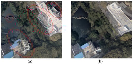
Figure 1.
The importance of visibility tests in texture reconstruction. (a) The textured model without visibility tests. (b) The textured model based on GPVC.
Xu et al. [19] introduced the hidden point removal (HPR) algorithm [20] to determine a face’s visibility. If the inversion of a face’s center lies on the convex hull of a mesh’s vertices and a given viewpoint, then the face is fully visible from that viewpoint. However, HPR was initially proposed to compute a point’s visibility in a point cloud; applying the algorithm to determine a face’s visibility in a 3D mesh is insufficient. Even if the center of a face is visible, the face can still be occluded (as shown in Figure 2a).
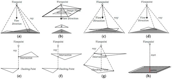
Figure 2.
Visibility issues that available methods fail to handle. The visible faces are drawn with solid lines, and the occluded faces are drawn with dotted lines and filled with shadow. Occlusion detection based on HPR is unable to identify the occluded face in (a). The projection-based approach incorrectly marks the occluded face in (b) as visible. Without dense tracing, the ray-tracing method cannot identify the occluded faces in (a,c,d). In addition, ray tracing will incorrectly determine the visible faces in (e–g) as occluded. Without an appropriate bias, it is difficult to compute the correct visibility between two close faces in (h) through ray-tracing and shadow-mapping approaches.
Pages et al. [13] used a projection-based approach to handle the occlusion problem. If one vertex of face is projected inside the projection area of face and lies between and a given viewpoint, then is occluded by . However, this technique only works in the occlusion condition, as depicted in Figure 3. If none of ’s vertices are projected inside (as shown in Figure 2b), then will be incorrectly determined as visible.
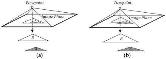
Figure 3.
Occlusion conditions in which the projection-based approach can work. (a) Face is entirely occluded by face . (b) Face is partially occluded by face .
According to the coherence of perspective transformation between 3D rendering and pinhole camera imagery, visibility checking in texture reconstruction can be regarded as a point-based visibility test [21,22]. Therefore, many related studies have applied ray-tracing [23,24,25,26] and distance-based comparison [14,16,27,28,29,30,31,32,33] of CG to solve the visibility issue in texture reconstruction.
The standard ray-tracing algorithm traces a virtual ray from a viewpoint to a point on a 3D surface; if an intersection between the viewpoint and the surface is found before reaching , then is occluded [34]. This algorithm was adopted in previous studies [15,35] to check visibility. In the implementation reported in Reference [14], the authors designed sparse tracing (three rays are cast to a face’s vertices) based on an open-source library [36]. Clearly, the occluded faces in Figure 2a,c,d will be inappropriately identified as visible by this type of implementation. In addition, when intersections occur on edges, as shown in Figure 2e,f, the visible faces will be identified as occluded. More importantly, all calculations involving ray tracing will introduce a bias [37], which requires an epsilon to reduce computation error. If the epsilon is small, then self-intersections may occur, resulting in visible regions becoming occluded; if the epsilon is large, then missed intersections may occur, resulting in occluded regions becoming visible. Thus, without an appropriate epsilon, it is very difficult to compute the correct visibility between two close faces, as shown in Figure 2h. In practice, a uniform grid data [23] or a hierarchical tree structure [24,25,26] is built to avoid needless intersection checking. However, when axis-aligned primitives exist, a greater number of intersection tests must be conducted [37].
In the distance-based comparison, given a viewpoint or a projection plane, among all points on a 3D surface that can be projected into the same pixel, the closest point to the viewpoint or the projection plane is visible. However, projecting all faces of a complex mesh and comparing the distance at each pixel [28] is a brute-force choice that requires hundreds of samplings. In previous studies [14,27,28,29], the projection plane of each view was tessellated with large grid cells to reduce samplings. Clearly, the visibility results based on this method are sensitive to the size of a grid cell. In previous studies [14,16,31,32,33], the authors applied the shadow-mapping algorithm [38,39,40] with the aid of the well-known Z-buffer. The distance of a given test point to the viewpoint is computed first, and then a comparison is made between the computed distance and the corresponding distance stored in the shadow map; if the computed distance is smaller, then the point is visible; otherwise, the point is occluded in shadow. In Reference [32], an empirical epsilon was added to the shadow map to reduce numerical error. However, the regular shadow mapping [38] suffers from the shadow acne artifact, which refers to erroneous self-shadowing [39]. Sampling the Z-buffer through the standard depth bias approach yields insufficient precision [41] because a constant depth bias does not work for every part of a geometry [40]. A small bias produces self-occlusion, and a large bias means missing occlusion. Thus, this Z-buffer-based approach is still limited by an uncontrollable bias. Without an appropriate bias, the correct visibility in Figure 2h is also in danger.
In this study, we propose a high-precision graphics pipeline-based visibility classification (GPVC) method to solve the visibility problem in texture reconstruction. The best advantage offered by GPVC is that visibility can be computed without introducing an improper bias. Our method consists of two stages. First, we design a shader-based rendering to generate each view’s initial visibility map (IVM) and record visible primitives in a shader storage buffer object. Three spatial properties of IVMs are excavated to form our visibility classification mechanism. Second, we propose two algorithms, namely, lazy-projection coverage correction (LPCC) and hierarchical iterative vertex-edge-region sampling (HIVERS), to classify the visible primitives into fully visible or partially visible primitives. Compared with per-primitive checking, the advantage of LPCC is that LPCC only handles the visible primitives that are stored. Another breakthrough provided by LPCC is that we take the polygon rasterization principle and rasterization error into account, which has not been considered in other fragment-based visibility tests. HIVERS is proposed to identify a primitive’s visibility on an arbitrary surface (manifold or nonmanifold) with fewer samplings.
The remainder of this paper is organized as follows. Section 2 describes the proposed method. Section 3 presents the implementation details in the graphics pipeline. Experimental results are presented in Section 4. Improvement of the proposed method is discussed with related studies in Section 5. Finally, Section 6 presents conclusions.
2. Graphics Pipeline-Based Visibility Classification
In this section, we provide the details of GPVC. First, IVMs are generated in the fixed graphics pipeline. Second, visibility classification is executed in the parallel computation stage. The framework of GPVC is depicted in Figure 4.
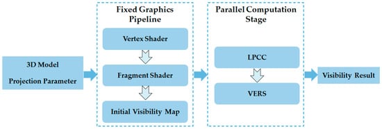
Figure 4.
The framework of GPVC.
2.1. IVM Generation
Unlike the Z-buffer-based methods used in [14,16,31,32,33], in which the shadow maps store the closest depth values, IVMs of GPVC store visible faces’ indexes as pixels. GPVC draws inspiration from digital camera photography, and we use two techniques to ensure that IVMs record the visible pixels coincident with digital images. First, in the XY plane, we design a shader-based rendering to achieve the locational coherence of corresponding pixels. The implementation mechanism of the shader-based rendering is described in Section 3. Second, in the Z-direction, we use the reversed projection [41] to avoid Z-fighting [42,43] and improve the precision of the Z-buffer. We explain the generation of IVMs according to the rasterization principle and present three spatial properties of IVMs.
2.1.1. Z-Buffer Precision Improvement
The default perspective projection matrix in OpenGL is symmetric, which is defined as
Thus, the nonlinear mapping relationship between the z-component of the eye coordinate and the stored in the Z-buffer can be expressed as
In Formula (2), and when is within , or and when is within , where is the depth value of the far plane and is the depth value of the near plane .
According to Formula (2), the z-component of the normalized device coordinate will be distributed in the symmetrical interval ; thus, has decreasing precision as points move away from a viewpoint (as shown in Figure 5a). To avoid this drawback, we use the asymmetric projection matrix in DirectX instead of the default configuration in OpenGL.
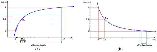
Figure 5.
Depth distribution in the Z-buffer. (a) Depth distribution in the default Z-buffer; and (b) depth distribution in the reversed Z-buffer.
Therefore, we obtain
In this manner, is distributed over the asymmetric interval, in which the near plane is mapped to 1, and the far plane is mapped to 0. To distribute the effective depths in the range with higher precision, i.e., close to 0 (as shown in Figure 5b), we design a “zero near plane” configuration; we compute and according to a 3D surface’s bounding box and a view’s projection parameter (as shown in Figure 6) and then pull as close to the viewpoint as possible. Formula (5) describes the mapping relationship of our implemented Z-buffer.
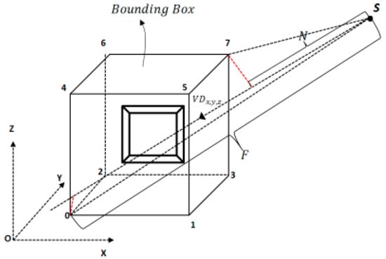
Figure 6.
Computing the near and far planes according to a 3D surface’s bounding box and a view’s projection parameter. : viewpoint; : normalized view direction. The near and far planes are equal to the projection length along the view direction.
2.1.2. IVM Generation and Spatial Properties
Rasterization in CG converts vectorial geometries to discrete fragments. An efficient and simple algorithm used in rasterization is the linear edge function (LEF) [44]. Given a triangle whose vertices are in the counterclockwise orientation and a fragment to be tested, LEF is defined as
- if the center of is to the left of one edge;
- if the center of is on one edge;
- if the center of is to the right of one edge.
where denotes the edge formed by vertices , is the center of . Thus, if , then is an inner fragment of (as shown in Figure 7). The fragment value of is computed as
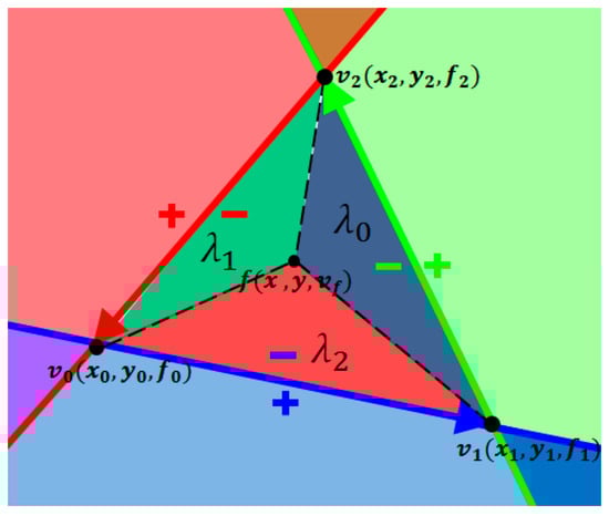
Figure 7.
LEF-based triangle rasterization.
In Formulas (7) and (8), represents the signed area of ; are the barycentric coordinates of ; are the attribute values associated with the three vertices of ; and are the clip coordinates.
After rasterization, visible fragments are written to target buffers if early fragment tests are enabled [45]. In other words, visible parts of 3D surfaces are projected as those visible fragments. We use an item buffer to store the visible primitives’ indexes as pixels. In this manner, the continuous visibility issue in 3D space is converted to a discrete visibility issue in 2D space [22,34]. IVMs formed by the visible fragments have three spatial properties, which is the foundation of our visibility classification.
Handiness: Only visible primitives are recorded, and fully occluded primitives are discarded.
Coherence: Visibility property of a face in 3D space remains unchanged in IVMs.
Continuity: Fragments’ values within a fully visible primitive are uniform; otherwise, this primitive is partially visible (as shown in Figure 8).
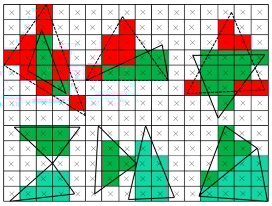
Figure 8.
The continuity of IVMs. The fully visible primitives are drawn with solid lines and filled with green pixels; the partially visible ones are drawn with dotted lines and filled with red pixels.
2.2. Visibility Classification
Visibility classification based on IVMs marks a primitive with a fully visible or partially visible label, which represents the visibility issue in 2D space. The 2D visibility computation has been treated as hundreds of polygon-polygon intersection tests in [9,10]. Instead, based on the spatial properties of IVMs, lazy-projection coverage correction (LPCC), and hierarchical iterative vertex-edge-region sampling (HIVERS) are proposed to improve visibility computation.
2.2.1. Lazy-Projection Coverage Correction
(1) Lazy Projection
The backface culling and frustum culling are the two classical strategies that are widely used to reduce needless visibility tests. After the processing of these methods, remaining faces of a 3D surface in the viewshed consist of fully visible faces , partially visible faces and fully occluded faces . The related methods used in texturing need to handle each face’s visibility in . Instead, lazy projection is proposed to avoid addressing the faces’ visibilities in . Based on the fact that fully occluded faces are automatically discarded by the depth test, we use a shader storage buffer object, which is a continuous array, to record visible faces’ indexes at corresponding subscripts (as shown in Figure 9). Given a visible face stored in the array, we project the face onto IVMs to obtain its initial projection coverage (IPC). In this manner, we only process the faces in .
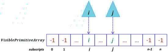
Figure 9.
Recording visible faces’ indexes in a shader storage buffer object.
(2) Projection Coverage Correction
After lazy projection, visibility judgment for a face only needs to apply the IVMs’ continuity. However, due to the following two concerns, we should provide some correction to a face’s IPC during visibility classification. First, the fragments whose centers lie on an edge do not always belong to a face (as shown in Figure 10). Second, the rasterization of an edge contains errors (see Figure 11). These two details interfering with visibility computation are overlooked by the fragment-based visibility tests in References [14,16,31,32,33]. Without considering these details, the continuity of a primitive will be destroyed.
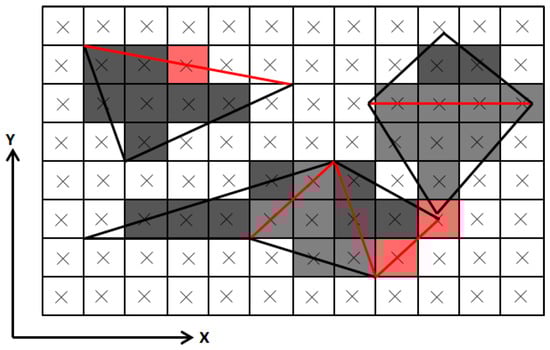
Figure 10.
The top-left rule used to rasterize edges that cross fragments’ centers. The edges in red are the ones that cross fragments’ centers. The gray brightness of a fragment denotes the triangles to which the fragment belongs. The red fragments whose centers lie on the edges do not belong to the corresponding triangles because the edges are not left edges.
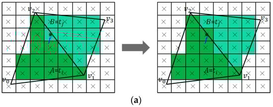
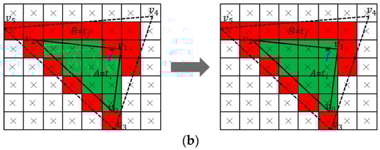
Figure 11.
Rasterization error correction. (a) Rasterization error correction between two adjacent triangles. (b) Rasterization error correction between two overlapped triangles.
In CG, rendering adjacent primitives’ shared edges twice is avoided by using rules to maintain consistency. The top-left rule (TLR) [46] is the criterion used in Direct3D to address this situation. Given a triangle whose vertices are in the counterclockwise orientation, if an edge ( is start, and is end) is perfectly horizontal, and the x-coordinate of is smaller than the x-coordinate of , then is a top edge; if the y-coordinate of is smaller than the y-coordinate of , then is a left edge. If a fragment’s center lies on a top edge, then the fragment belongs to the triangle that is below the top edge; if the center lies on a left edge, then the fragment belongs to the triangle that is to the right of the left edge (see Figure 10).
The rasterization error of edges often has little impact on the visual effect, but is nonnegligible in fragment-based visibility tests. As depicted in Figure 11, the rasterization error of edges indicates that a fragment within triangle is rasterized incorrectly as one of triangle . In our study, we find that the pixel offset caused by the rasterization error remains within (. Thus, we propose the following Algorithm 1. LPCC to recover the correct continuity of a visible primitive.
| Algorithm 1. LPCC |
| Definition: Given a visible triangle ti (i represents the index value of ti), IPCi represents the initial projection coverage of ti, f is one fragment crossed by each edge of triangle ti, vf is the fragment value of fragment f, and di is the distance from the viewpoint to f’s center in the plane of triangle ti. Function LPCC(ti): project ti and get IPCi foreach f crossed by each edge of ti do if f belongs to ti and vf ≠ i then j ← vf project and get if does not belong to then modify the value of fragment as else if then modify the value of fragment as end if end if end foreach |
Algorithm 1 consists of the following steps:
- Use LEF and TLR to judge whether a given fragment belongs to . If not, judge next fragment; otherwise, go to step 2
- Determine whether the value of fragment equals ’s index value . If yes, go to step 1; otherwise, go to step 3.
- Determine whether is an inner fragment of triangle . If not, is an exceptional fragment of triangle , then modify the value of fragment as (as shown in Figure 11a); otherwise, go to step 4.
- Determine whether triangle is in front of triangle at ’s center. If yes, is an exceptional fragment of triangle , then modify the value of fragment as (as shown in Figure 11b); otherwise, go to step 1.
2.2.2. Hierarchical Iterative Vertex-Edge-Region Sampling
HIVERS aims to identify a primitive’s visibility with fewer samplings. Based on the continuity of IVMs, if a primitive is considered to be fully visible, then must satisfy the following conditions.
Vertex visibility condition (VVC): the inner fragments corresponding to ’s vertices maintain a consistent value (see Figure 12a).
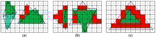
Figure 12.
The description of VVC, EVC and RVC. (a) VVC: the fully visible primitives satisfy VVC, while the partially visible primitives do not. (b) EVC: the fully visible primitives satisfy EVC, while the partially visible primitives do not. (c) RVC: the fully visible primitives satisfy RVC, while the partially visible primitives do not.
Edge visibility condition (EVC): the inner fragments corresponding to ’s edges maintain a consistent value (see Figure 12b).
Region visibility condition (RVC): the inner fragments within ’s subregions maintain a consistent value (see Figure 12c).
The three conditions are necessary to define a fully visible primitive. In addition, according to the continuity of IVMs and the spatial structure of a manifold surface, we can make the following inference.
Inference 1: If a given primitive of a manifold surface satisfies VVC and EVC, then this primitive is fully visible; otherwise, the primitive is partially visible. In other words, we only need to sample the inner fragments corresponding to ’s vertices and edges in a manifold surface. We denote this inference as VES.
To be compatible with the occlusion situations in nonmanifold surfaces, we integrate VVC, EVC and RVC to form HIVERS. As depicted in Figure 13, at each level of HIVERS, the three conditions are checked in order; we call this process one iteration at one level. The detailed procedure of Algorithm 2. HIVERS is as follows.
| Algorithm 2. HIVERS |
| Definition: Given a visible triangle , is the barycenter of , fv represents is fully visible and pv represents is partially visible. Function : if does not satisfy VVC or EVC then return end if if all fragments within have been sampled then return else do subdivide into subregions {} acorrding to use to address {} recursively end if |
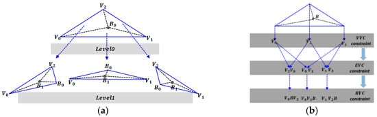
Figure 13.
The framework of HIVERS. (a) The hierarchical structure of HIVERS. (b) One iteration at one level.
Algorithm 2 consists of the following steps:
- Determine whether triangle satisfies VVC. If not, then is partially visible; otherwise, go to step 2.
- Determine whether satisfies EVC. If not, then is partially visible; otherwise, go to step 3.
- Check whether all fragments within have been sampled. If yes, is fully visible; otherwise, go to step 4.
- Subdivide into subregions {} according to ’s barycenter , and address each subregion from step 1 to step 3. If any of the subregions is partially visible, then is partially visible; if all of the subregions are fully visible, then is fully visible.
3. Implementation in Graphics Pipeline
The proposed framework is implemented in the graphics pipeline based on OpenGL. The implementation consists of IVM generation in the fixed graphics pipeline and visibility classification in the parallel computation stage.
3.1. IVM Generation in Fixed Graphics Pipeline
Zhang et al. [47] simulated digital photography by passing the projection parameter to the default graphics pipeline, which may produce the off-center projection dislocation. Instead, we present a shader-based rendering to generate IVMs. Given a 3D object and an undistorted digital image, the transformation from 3D to 2D in CV can be expressed as
Formula (9) is equivalent to
In Formula (10), is the rotation matrix, is the viewpoint, and are the camera’s focal length expressed in the pixel unit, and is the principal point.
The transformation from 3D to 2D in CG can be expressed as
In Formula (11), is the matrix that transforms the object coordinate into the eye coordinate ; is the matrix that transforms the eye coordinate into the clip coordinate ; is the normalized device coordinate, where when the viewport’s origin is lower-left and when the viewport’s origin is upper-left; is the window coordinate; represents the viewport’s lower-left corner.
To relate Formula (10) with Formula (11), our shader-based rendering is designed as follows. First, according to Formula (10), we compute one vertex’s projection in the vertex shader. Second, we let and in Formula (10) be and in Formula (11), respectively; we then substitute and into Formula (11) to compute as
In Formula (12), is normalized to improve rendering efficiency, is computed according to Formula (4) to improve the Z-buffer’s precision, and viewport size is replaced with image size. Finally, in the fragment shader, we use an off-screen texture to store visible fragments and a shader storage buffer object to record visible primitives’ indexes at the corresponding subscripts (as shown in Figure 9).
3.2. Visibility Classification in Parallel Computation Stage
The parallel computation stage in OpenGL exists as the compute shader. Compared with OpenCL, the compute shader is a lightweight framework with less complexity and interoperability with shared resources. This stage is completely independent of any predefined graphics-oriented semantics. The compute shader can read and modify OpenGL buffers and images. The tool is, therefore, able to modify data that are the input or output of the fixed graphics pipeline. Due to the independence between the compute shader and the fixed graphics pipeline, we must consider synchronization. We disable the compute shader after completing visibility classification in the current frame and recover it after IVM generation in the next frame.
The following data are passed into our compute shader. (1) Multiview’s IVMs. One view’s IVM is passed as an “image2D” object. (2) and projection parameter. The projection parameter is stored as a uniform matrix. (3) 3D model data. Vertices and faces are stored in two shader storage buffer objects. (4) Face and vertex number. To classify visibility between multiple models, the face and vertex numbers of each model are stored in a uniform buffer object, which act as search indexes (as shown in Figure 14).
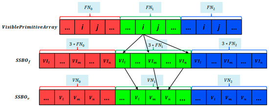
Figure 14.
Visiting a specific face in multiple models. represents one model’s face number, represents one model’s vertex number, represents one face’s vertices’ indexes, represents one vertex’s coordinate, is the shader storage buffer object storing faces and is the shader storage buffer object storing vertices.
In the compute shader, our visibility classification proceeds as follows. Each visible primitive stored in is visited by an independently parallel thread. In each thread, our visibility classification is executed.
4. Experiments
The following tests are conducted in our experiments. With respect to accuracy, we use related methods to detect visibility for three synthetic models. The visibility of the three synthetic models is known from a predefined viewpoint. With respect to efficiency, we compare the related methods’ number of processed faces, sampling count, and time consumption. With respect to texture reconstruction, comparisons between GPVC and other available libraries and software are made. The key steps of GPVC are also presented in our experiments. The experimental platform is Win8.1 x64 OS, with 16 GB computer memory, I7 CPU (2.5 GHz, 4 cores, and 8 threads) and a GTX 860 M video card.
4.1. IVM Generation
4.1.1. Z-Buffer Precision Improvement
Figure 15 shows the visual effect when rendering very close faces based on different Z-buffer configurations. The default Z-buffer with the symmetric projection results in the Z-fighting problem due to the infinite precision. The reversed Z-buffer with the asymmetric projection used in GPVC exhibits good performance to avoid the problem, which ensures the continuity of IVMs. The format of the Z-buffer used in this paper is set to a 32-bit floating point.
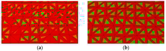
Figure 15.
Comparison of the visual effect between the default Z-buffer and the reversed Z-buffer. (a) Rendering effect of the default Z-buffer. (b) Rendering effect of the reversed Z-buffer used in GPVC.
4.1.2. Shader-Based Rendering
In this section, we demonstrate the significance of our shader-based rendering in the simulation of digital photography. To present the feature boundaries clearly, we fuse the five views, rendering images with the corresponding digital images, as shown in Figure 16. To prove the validity of our approach, we compare our shader-based rendering with the default rendering in detail. As shown in Figure 17, the default rendering cannot accurately simulate the off-center perspective projection, resulting in distinct object dislocations relative to the digital images. Compared with the default approach, the shader-based rendering can maintain the corresponding objects spatially aligned.
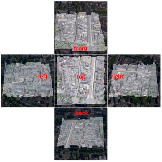
Figure 16.
The fusion of rendering images and oblique digital images from five views.
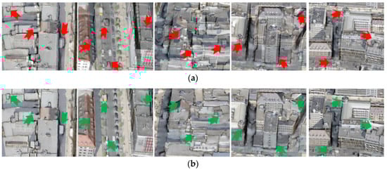
Figure 17.
Detailed contrasts between the shader-based rendering and the default rendering. (a) Detailed features in the default rendering images. (b) Detailed features in the shader-based rendering images.
4.2. Visibility Classification
4.2.1. Visibility Accuracy Statistics
We design three synthetic models to examine the accuracy of related methods. As shown in Figure 18a, each model consists of two uneven terrain layers (upper layer and lower layer ); each layer is a triangulation network containing 4082 faces. For , the vertical distance between and is 0.01 m; for , the vertical distance is 1 m; and for , the vertical distance is 100 m. Given a predefined top view (the viewpoint is 6100 m from the center of a synthetic model), the triangles of are fully visible, and the triangles of are partially occluded (as shown in Figure 18b). Based on these features, we present related methods’ performances.
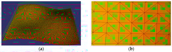
Figure 18.
Synthetic models. (a) Global view. (b) Top view in detail.
(1) Shadow-Mapping Algorithm
The nonlinear depth distribution in the Z-buffer is highly sensitive to the projection matrix, particularly to the near and far planes. Without the loss of generality, we use two projection configurations to present the performance of the shadow-mapping algorithm. Symmetric projection configuration (SPC): the symmetric projection matrix with a pair of adaptive planes. The adaptive planes are computed according to Figure 6. Asymmetric projection configuration (APC): the asymmetric projection matrix with a “zero near plane” and an adaptive far plane; this mechanism is recommended by our GPVC. In this design, given the predefined top viewpoint, the two projection configurations are both sufficient to avoid Z-fighting when rendering the synthetic models. Table 1 and Table 2 show the accuracy statistics. The is used to determine whether a pixel within a face is visible: if , then the pixel is visible; otherwise, the face is occluded. We attempt to enumerate the from 0.1 to 1 × 10⁻¹³ to prove the difficulty of choosing an appropriate bias. In each enumeration, the new is reduced to half of the original value. For simplicity, in the following tables, represents the visible face number, represents the occluded face number, and represents the detection accuracy.

Table 1.
Accuracy statistics of the shadow-mapping algorithm with SPC.
Table 2.
Accuracy statistics of the shadow-mapping algorithm with APC.
(2) Ray-Tracing Algorithm
The ray-tracing algorithm used here is an open-source library [36], which is employed by Waechter et al. [15] with a sparse sampling implementation. Under the sparse sampling mode, only the three vertices of a triangle are checked; if one vertex is occluded, then the triangle is invisible. The sparse sampling does not work well for our synthetic models; thus, based on the library, we design a dynamic dense sampling (as shown in Figure 19). The dynamic dense sampling indicates that the sampling points within a triangle remain at the centers of the inner fragments of a triangle. Because all calculations involving ray tracing will introduce a bias, we need an to determine a checking point’s visibility: If the distance between the checking point and the first intersection point is smaller than the , then the checking point is visible. We also enumerate the from 0.1 to 1 × 10⁻¹³ to present the detection accuracy with different biases. Table 3 and Table 4 show the accuracy statistics.
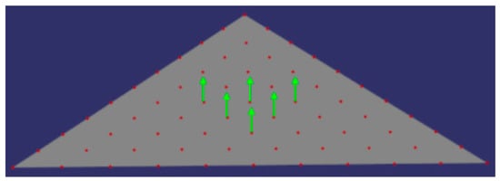
Figure 19.
Ray tracing with the dynamic dense sampling.
Table 3.
Accuracy statistics of ray tracing with the sparse sampling.
Table 4.
Accuracy statistics of ray tracing with the dynamic dense sampling.
(3) GPVC
Visibility computation based on GPVC can be achieved without choosing an improper bias. The accuracy of GPVC reaches 100% after projection coverage correction. Table 5 and Table 6 show the accuracy statistics.
Table 5.
Accuracy statistics of GPVC before projection coverage correction.
Table 6.
Accuracy statistics of GPVC after projection coverage correction.
4.2.2. Visibility Efficiency Statistics
We use a manifold mesh (611,055 faces) reconstructed from 43 views to present the efficiency of related methods. Table 7, Table 8 and Table 9 are the statistics pertaining to the number of processed faces, sampling count and time consumption. The number of processed faces represents the total number of faces after backface culling and frustum culling in 43 views. The sampling count represents the total sampling number during computing visibility for the processed faces.
Table 7.
Efficiency statistics of the shadow-mapping algorithm.
Table 8.
Efficiency statistics of the ray-tracing algorithm.
Table 9.
Efficiency statistics of GPVC.
4.3. Texturing Contrast
In this section, we apply related methods to multiview-based texture reconstruction and compare the textured models generated by available libraries and software. We use two datasets to prove our method’s superiority. The first dataset pertains to the campus of Wuhan University (as shown in Figure 20a), and the second is provided by ISPRS and EuroSDR (as shown in Figure 20b). First, we use the famous business software ContextCapture to reconstruct the triangular meshes of the two datasets. Next, we use related methods to compute the visibility of each view. Finally, we use graph cuts to select the optimal fully visible textures.
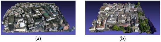
Figure 20.
The textured models based on GPVC. (a) The textured model of Wuhan University. (b) The textured model reconstructed from the ISPRS and EuroSDR datasets.
5. Discussion
In this study, a graphics pipeline-based visibility classification (GPVC) method is proposed to improve the visibility handling involving multiview-based texture reconstruction. Experimental results demonstrate that our method outperforms related methods and available tools.
During IVM generation, we use the reversed Z-buffer and the shader-based rendering to ensure the accuracy of IVMs. The reversed Z-buffer designed in this paper can avoid Z-fighting when rendering very close faces (as shown in Figure 15), which guarantees the continuity of IVMs. Our shader-based rendering is proposed to achieve the locational coherence of corresponding objects between rendering images and digital images (as shown in Figure 17). The default rendering used in [47] fails to maintain the corresponding objects spatially aligned (as shown in Figure 17a). In our study, givenUAV image whose principal point is at, the off-center projection dislocation can reach more than 50 pixels in the x-axis direction and 90 pixels in the y-axis direction. The dislocation causes some visible primitives to exit the viewshed or that some invisible ones enter the viewshed.
Compared with the shadow-mapping [14,16,31,32,33] and ray-tracing [15,35] methods used in texturing, the main contribution of GPVC is that visibility computation is performed without a bias. To demonstrate the shortcomings of the bias-based methods, we design three models with known visibility from a predefined viewpoint. As shown in Table 1, the shadow-mapping algorithm with the symmetric projection configuration only works well when the epsilon remains in the ranges specified by enumeration (3.05 × 10⁻⁶~1.22 × 10⁻⁵ for synthetic model A, 3.91 × 10⁻⁴~0.00156 for synthetic model B, 3.91 × 10⁻⁴~0.1 for synthetic model C). As the two layers of the synthetic models move closer, the optimal epsilon becomes increasingly difficult to specify. The reason is that the computed depths and the depths stored in the Z-buffer tend to be approximate, requiring a smaller epsilon to distinguish the correct visibility. If the selected epsilon increases, certain occluded faces are identified as visible; if the selected epsilon decreases, certain visible faces are identified as occluded. This problem becomes more serious when using the shadow-mapping algorithm with the asymmetric projection configuration, as shown in Table 2, only when the epsilon is in the range (1 × 10⁻¹³~4.77 × 10⁻⁸) is the performance satisfactory for synthetic model C; using other epsilons misses many occlusions. The reason is that the computed and stored depths are distributed over the range with more precision (very close to 0.0). Only a very small epsilon can work, even if the two layers of synthetic model C are distant. In this respect, the shadow-mapping algorithm with the asymmetric projection configuration is unfit to compute visibility in texture reconstruction. As shown in Table 3 and Table 4, the dense ray tracing outperforms the sparse ray tracing for our synthetic models. The reason is that our three synthetic models are not manifold, and the sparse ray tracing fails to identify certain occluded faces. Within certain biases (1.95 × 10⁻⁴~0.006 for synthetic model A, 1.95 × 10⁻⁴~0.1 for synthetic models B and C), the accuracy of the dense ray tracing can reach 100%. However, in the dense ray-tracing mode, increasingly more faces are labeled as occluded if the epsilon decreases outside of the abovementioned ranges. This effect results from the ability of an increased number of tracings to generate more self-intersections. Compared with that of the two methods mentioned above, our GPVC’s performance is robust for the three models due to the use of the continuity of IVMs. After projection coverage correction, the accuracy of GPVC can reach 100% (as shown in Table 5 and Table 6). We also apply our projection coverage correction to the shadow-mapping algorithm and obtain the following results. With the aid of our projection coverage correction, the accuracy of the shadow-mapping algorithm with the symmetric projection configuration (epsilon = 0.00156 for synthetic model B, epsilon remains in 7.81 × 10⁻⁴~0.1 for synthetic model C) can reach 100%; the accuracy of the shadow-mapping algorithm with the asymmetric projection configuration (epsilon remains in 1.82 × 10⁻¹³~1.46 × 10⁻¹² for synthetic model C) can also reach 100%.
To demonstrate the improvement of GPVC in texturing, we present many comparisons pertaining to textured models generated by related methods, open-source libraries (MVS-Texturing) and business software (ContextCapture). As shown in Figure 21, Figure 22, Figure 23, Figure 24 and Figure 25, the detailed areas are the three parts of one textured model reconstructed from the ISPRS and EuroSDR datasets. Unlike our synthetic models (in one synthetic model, the distance between two layers is fixed), the urban models reconstructed from multiview images have dense faces and complex geometry structures. In the case of the shadow-mapping algorithm and ray-tracing methods, some areas’ visibility can be computed correctly, and textures are mapped well by using a given bias. However, this bias is not robust for every part of the complex model. Thus, many areas are mapped with inaccurate textures (as depicted in the red boxes in Figure 21, Figure 22, Figure 23 and Figure 24). The textured results based on the shadow-mapping algorithm with the symmetric projection configuration are highly sensitive to the selected bias because the depths are distributed in [0, 1] dispersedly; thus, a small change in the bias can generate different visibility, producing different textures. As shown in Figure 21, the texturing gets better as the used bias increases because more visible textures are correctly detected. While the textured results based on the shadow-mapping algorithm with the asymmetric projection configuration appear to be insensitive to the bias because the depths are distributed at approximately 0.0 densely; thus, a large change in the epsilon has little effect on the visibility results, producing nearly unchanged textures. As shown in Figure 22, because the four used biases are not sufficiently small to identify the occluded faces, the occluded textures are mapped to the corresponding areas. The left screenshot in Figure 22 is textured with the correct color because the corresponding area is a nearly flat structure without complex occluders, thus the identified visible textures are mapped to the correct locations. When comparing the texturing in Figure 22 with the one in Figure 25a, it can be seen that the texturing based on the shadow-mapping algorithm with the asymmetric projection configuration is nearly as same as the one without visibility tests. The reason is that almost all of the faces are detected as visible by the shadow-mapping algorithm with the asymmetric projection configuration, which is nearly equivalent to skipping visibility tests. Compared with that afforded by the sparse ray tracing, the improvement of the dense ray tracing is not as obvious. The reason is that for a manifold surface, most faces’ correct visibility can be determined by checking three vertices with an appropriate bias. In some cases, the dense ray tracing is worse than the sparse ray tracing (as shown in Figure 23c and Figure 24c). The reason is that a face’s visibility tends to be incorrect as sampling time grows without an appropriate bias. If the bias is small, then self-occlusions occur, and visible faces become invisible, leaving holes in the textured models (as shown in Figure 23a–c and Figure 24e–g); if the bias is large, then occluded faces become visible, leaving incorrect textures on the textured models. Figure 25 shows the performance of our method. Without visibility tests, there are serious deviations contained in the right two screenshots (see Figure 25a) due to the error mapping of occluded textures. Before projection coverage correction, the textured results contain some artifacts because the optimal textures are not identified as visible, and some other inadequate visible textures have a chance to be mapped (as shown in Figure 25b). One concern is that given a manifold mesh, without projection coverage correction, the textured areas generated by HIVERS and VES are the same. The reason is that the rasterization error only occurs near the edges of polygons; if a visible triangle face contains exceptional fragments, it will be detected as invisible by HIVERS and VES. After projection coverage correction, the artifacts disappear. The only difference of the texture areas within the green boxes in Figure 25c,d results from the corresponding area of the reconstructed mesh containing nonmanifold structures (as shown in Figure 26, the nonmanifold parts are trees that are not reconstructed completely). Thus, after projection coverage correction, the target faces’ visibility computed by HIVERS and VES is not the same. While the other two textured areas in Figure 25 are strictly manifold, the textured results of HIVERS and VES are the same. This finding proves the validity of Inference 1.
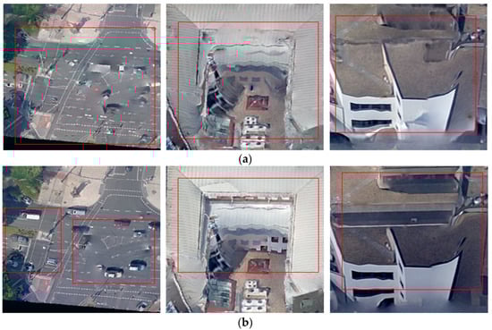
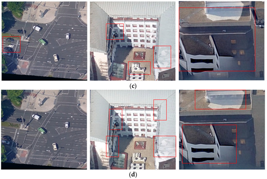
Figure 21.
Textured areas based on the shadow-mapping algorithm with SPC. (a) Textured areas when epsilon = 0.00001. (b) Textured areas when epsilon = 0.0001. (c) Textured areas when epsilon = 0.001. (d) Textured areas when epsilon = 0.01.
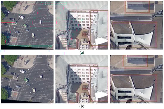
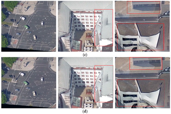
Figure 22.
Textured areas based on the shadow-mapping algorithm with APC. (a) Textured areas when epsilon = 0.00001. (b) Textured areas when epsilon = 0.0001. (c) Textured areas when epsilon = 0.001. (d) Textured areas when epsilon = 0.01.
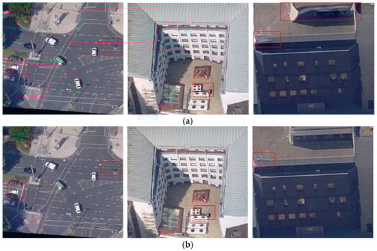
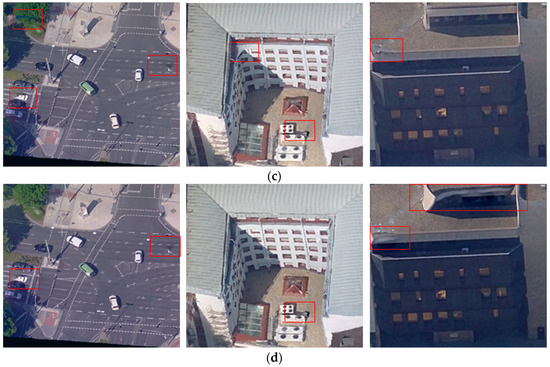
Figure 23.
Textured areas based on the sparse ray-tracing. (a) Textured areas when epsilon = 0.00001. (b) Textured areas when epsilon = 0.0001. (c) Textured areas when epsilon = 0.001. (d) Textured areas when epsilon = 0.01.
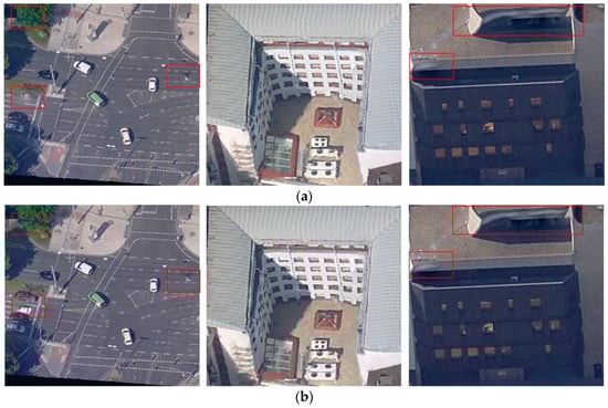
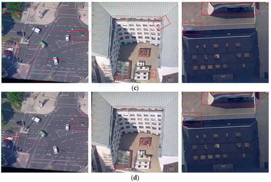
Figure 24.
Textured areas based on the dense ray-tracing. (a) Textured areas when epsilon = 0.00001. (b) Textured areas when epsilon = 0.0001. (c) Textured areas when epsilon = 0.001. (d) Textured areas when epsilon = 0.01.
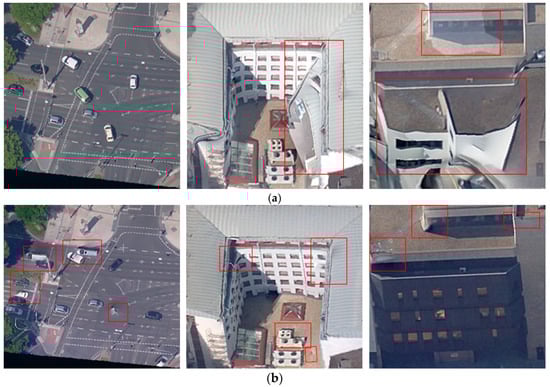
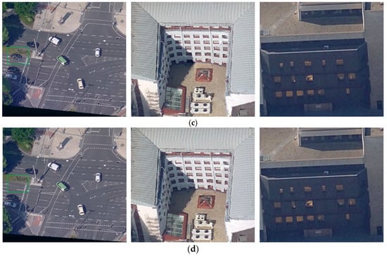
Figure 25.
Textured areas of our method. (a) Textured areas without visibility tests. (b) Textured areas based on GPVC but without projection coverage correction. (c) Textured areas based on GPVC with projection coverage correction (HIVERS). (d) Textured areas based on GPVC with projection coverage correction (VES).
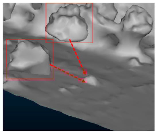
Figure 26.
The nonmanifold structures of the reconstructed mesh.
Figure 27, Figure 28 and Figure 29 presents texturing comparisons between GPVC and other software. It can be seen that the distortions, dislocations, and holes contained in the textured models generated by ContextCapture and MVS-Texturing result from the inaccurate selection of textures. In the textured models based on GPVC, these noises disappear, which proves the superiority of GPVC. GPVC attempts to compute the true visibility of each face on a surface. In other words, the accuracy of GPVC will not be affected by the artifacts of a reconstructed geometry. As shown in Figure 30a (to show the artifacts obviously, we enable each face’s normal during rendering), the reconstructed geometry contains many artifacts such as the distortions, uneven areas and fragments. And these artifacts still occur in the textured model. Some of the serious artifacts have an effect on their neighbors’ visibilities, resulting in the optimal textures being excluded, but the selected textures are still reasonable. Compared with the reconstructed geometry, no artifacts occur in the relatively accurate geometry in Figure 30b (the accurate geometry is extracted from the reconstructed geometry by using the method proposed by Verdie et al. [48]). Thus, fewer artifacts occur in the textured model. But there are still dislocations in the red boxes of Figure 30b. The reason is that the extracted geometry misses some occluders such as trees and roofs, and these occluders’ textures are mapped to the corresponding areas. From the above analysis, visibility tests based on GPVC and texturing are sensitive to the structures of reconstructed geometries.
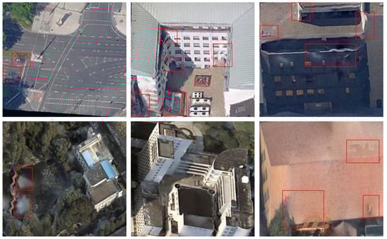
Figure 27.
Textured areas generated by ContextCapture.
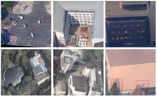
Figure 28.
Textured areas generated by MVS-Texturing [15].
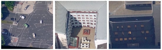
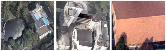
Figure 29.
Textured areas based on GPVC.
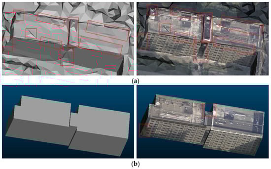
Figure 30.
Textured comparisons between inaccurate geometries and accurate geometries. (a) Left: An inaccurate reconstructed geometry; right: the reconstructed geometry’s texturing. (b) Left: The relatively accurate geometry extracted from the reconstructed geometry; right: the extracted geometry’s texturing.
In terms of efficiency, we present the statistics regarding the number of processed faces, sampling count and time consumption of related methods. As shown in Table 7, Table 8 and Table 9, the number of processed faces in GPVC decreases to nearly 1/3 of those in the shadow-mapping and ray-tracing methods. The reason is that our GPVC only handles the visible faces that are stored in the shader storage buffer object (as shown in Figure 9), while the other two methods must handle the visible and invisible faces. With respect to the sampling count, the sparse ray tracing has the lowest value because it only processes the three vertices of a triangle. The shadow-mapping algorithm with the symmetric projection configuration (epsilon = 0.00001) is second. The reason is that the epsilon in use is too small for the experimental mesh, and many faces are labeled as occluded after sampling a few inner fragments. As discussed above, the performance of the shadow-mapping algorithm with the asymmetric projection configuration is not insensitive to the selected epsilon; thus, this approach’s efficiency remains nearly unchanged. Compared with other methods, the improvement of GPVC with dense sampling is not as obvious. The reason is that many visible faces are identified as occluded by other bias-based methods without sampling all inner fragments. GPVC with dense sampling must sample all inner fragments of visible faces to ensure correct visibility. This situation can be improved by using HIVERS. Compared with dense sampling, the main function of HIVERS is that HIVERS can identify occluded faces with fewer samplings (as shown in Figure 31). Unlike the hierarchical structures used in References [24,25,26,49], in which hierarchy trees are built for a global scene as look-up indexes, the hierarchical structure of HIVERS decomposes a single triangle face into vertices, edges and subregions iteratively (see Figure 13). HIVERS samples the inner fragments corresponding to vertices and edges in each subregion to identify each face’s visibility. According to our Inference 1, HIVERS can be replaced by VES when addressing a manifold scene. VES not only performs well for a partially visible primitive but also avoids sampling all of the inner fragments within a fully visible primitive; thus, the improvement on the sampling count increases by nearly 1/3 (as shown in Table 9). In terms of time consumption, the shadow-mapping algorithm with the symmetric projection configuration requires more time as epsilon increases. The reason is that a larger epsilon produces more visible fragments, requiring more samplings to inspect a visible primitive. In contrast, although the sampling count increases as epsilon increases, the time cost of the ray tracing decreases. The reason is that a larger epsilon used in Reference [36] can reduce the traversal of hierarchy tree nodes and reach leaves with less time. However, the ray-tracing still exhibits the worst performance due to its limitation in finding intersections on a complex surface. Compared with the bias-based methods, GPVC exhibits good performance with respect to efficiency as well as accuracy. When deploying our visibility classification in the compute shader, the task can be performed within 0.2 s.
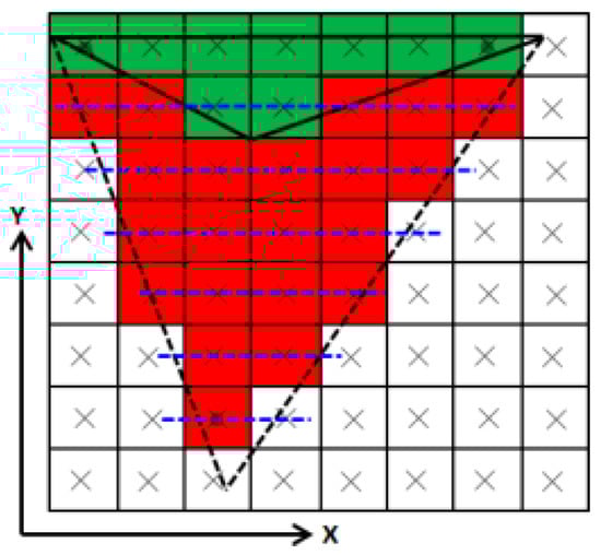
Figure 31.
The improvement of HIVERS. In the worst case, the dense sampling must traverse 20 fragments to identify the occluded primitive, while HIVERS only traverses 2 fragments.
6. Conclusions
Visibility computation is highly important in multiview-based texture reconstruction. However, the bias-based methods used in this field are unable to achieve a good performance for a complex surface. Thus, in this paper, we propose GPVC which does not depend on an uncontrollable bias, to make an improvement. According to our experimental results, GPVC outperforms the bias-based methods and other related libraries and software. Based on GPVC’s framework, certain applications, such as shadow generation, visibility picking, and visibility query, can also be derived.
Author Contributions
X.H. proposed the idea and wrote the manuscript; Q.Z. provided the experimental data; W.J. conceived and designed the experiments; and X.H. performed the experiments and analyzed the data.
Funding
This work was supported by the Key Technology program of China South Power Grid under Grant GDKJQQ20161187.
Acknowledgments
The authors would like to acknowledge the provision of the datasets by ISPRS and EuroSDR, released in conjunction with the ISPRS scientific initiative 2014 and 2015, led by ISPRS ICWG I/Vb.
Conflicts of Interest
The authors declare no conflict of interest.
References
- Jimenezdelgado, J.J.; Segura, R.J.; Feito, F.R. Efficient collision detection between 2d polygons. J. WSCG 2004, 12, 191–198. [Google Scholar]
- Feng, Y.T.; Owen, D.R.J. A 2d polygon/polygon contact model: Algorithmic aspects. Eng. Comput. 2004, 21, 265–277. [Google Scholar] [CrossRef]
- Greminger, M.A.; Nelson, B.J. A deformable object tracking algorithm based on the boundary element method that is robust to occlusions and spurious edges. Int. J. Comput. Vision 2007, 78, 29–45. [Google Scholar] [CrossRef]
- Huang, Y.; Essa, I.A. Tracking multiple objects through occlusions. In Proceedings of the IEEE Computer Society Conference on Computer Vision and Pattern Recognition, San Diego, CA, USA, 20–25 June 2005; pp. 1051–1058. [Google Scholar]
- Han, B.; Paulson, C.; Lu, T.; Wu, D.; Li, J. Tracking of multiple objects under partial occlusion. In Proceedings of the SPIE Defense, Security, and Sensing, Orlando, FL, USA, 5 May 2009. [Google Scholar]
- Yang, Q.; Wang, L.; Yang, R.; Stewenius, H.; Nister, D. Stereo matching with color-weighted correlation, hierarchical belief propagation, and occlusion handling. IEEE Trans. Pattern Anal. Mach. Intell. 2009, 31, 492–504. [Google Scholar] [CrossRef] [PubMed]
- Eisert, P.; Steinbach, E.G.; Girod, B. Multi-hypothesis, volumetric reconstruction of 3-d objects from multiple calibrated camera views. In Proceedings of the IEEE International Conference on Acoustics Apeech and Signal Processing, Phoenix, AZ, USA, 15–19 March 1999; pp. 3509–3512. [Google Scholar]
- Lee, Y.J.; Lee, S.J.; Park, K.R.; Jo, J.; Kim, J. Single view-based 3d face reconstruction robust to self-occlusion. EURASIP J. Adv. Signal Process. 2012, 2012, 176. [Google Scholar] [CrossRef]
- Kuffner, J.J.; Nishiwaki, K.; Kagami, S.; Inaba, M.; Inoue, H. Footstep planning among obstacles for biped robots. In Proceedings of the IEEE/RSJ International Conference on Intelligent Robots and Systems, Maui, HI, USA, 29 October–3 November 2001; pp. 500–505. [Google Scholar]
- Ahuja, N.; Chien, R.T.; Yen, R.; Bridwell, N. Interference detection and collision avoidance among three dimensional objects. In Proceedings of the First Annual National Conference on Artificial Intelligence, Stanford, CA, USA, 18–21 August 1980; pp. 44–48. [Google Scholar]
- Nakamura, T.; Asada, M. Stereo sketch: Stereo vision-based target reaching behavior acquisition with occlusion detection and avoidance. In Proceedings of the IEEE International Conference on Robotics and Automation, Minneapolis, MN, USA, 22–28 April 1996; pp. 1314–1319. [Google Scholar]
- Jiang, S.; Jiang, W. Efficient sfm for oblique uav images: From match pair selection to geometrical verification. Remote Sens. 2018, 10, 1246. [Google Scholar] [CrossRef]
- Pages, R.; Berjon, D.; Moran, F.; Garcia, N.N. Seamless, static multi-texturing of 3d meshes. Comput. Graph. Forum 2015, 34, 228–238. [Google Scholar] [CrossRef]
- Zhang, W.; Li, M.; Guo, B.; Li, D.; Guo, G. Rapid texture optimization of three-dimensional urban model based on oblique images. Sensors 2017, 17, 911. [Google Scholar] [CrossRef] [PubMed]
- Waechter, M.; Moehrle, N.; Goesele, M. Let there be color! Large-scale texturing of 3d reconstructions. In Proceedings of the 13th European Conference on Computer Vision, Zurich, Switzerland, 6–12 September 2014; pp. 836–850. [Google Scholar]
- Pintus, R.; Gobbetti, E.; Callieri, M.; Dellepiane, M. Techniques for seamless color registration and mapping on dense 3d models. In Sensing the Past; Springer: Berlin, Germany, 2017; pp. 355–376. [Google Scholar]
- Symeonidis, A.; Koutsoudis, A.; Ioannakis, G.; Chamzas, C. Inheriting texture maps between different complexity 3d meshes. ISPRS Ann. Photogramm. Remote Sens. Spat. Inf. Sci. 2014, II-5, 355–361. [Google Scholar] [CrossRef]
- Frueh, C.; Sammon, R.; Zakhor, A. Automated texture mapping of 3d city models with oblique aerial imagery. In Proceedings of the 2nd International Symposium on 3D Data Processing, Visualization and Transmission, Thessaloniki, Greece, 6–9 September 2004; pp. 396–403. [Google Scholar]
- Xu, L.; Li, E.; Li, J.; Chen, Y.; Zhang, Y. A general texture mapping framework for image-based 3d modeling. In Proceedings of the 17th IEEE International Conference on Image Processing, Hong Kong, China, 26–29 September 2010; pp. 2713–2716. [Google Scholar]
- Katz, S.; Tal, A.; Basri, R. Direct visibility of point sets. ACM Trans. Graph. 2007, 26, 343–352. [Google Scholar] [CrossRef]
- Cohenor, D.; Chrysanthou, Y.; Silva, C.T.; Durand, F. A survey of visibility for walkthrough applications. IEEE Trans. Vis. Comput. Graph. 2003, 9, 412–431. [Google Scholar] [CrossRef]
- Bittner, J.; Wonka, P. Visibility in computer graphics. Environ. Plan. B Plan. Des. 2003, 30, 729–755. [Google Scholar] [CrossRef]
- Franklin, W.R.; Chandrasekhar, N.; Kankanhalli, M.; Seshan, M.; Akman, V. Efficiency of uniform grids for intersection detection on serial and parallel machines. In New Trends in Computer Graphics-CGI’88; Springer: Geneva, Switzerland, 1988; pp. 288–297. [Google Scholar]
- Yu, B.T.; Yu, W.W. Image space subdivision for fast ray tracing. In Proceedings of the SPIE’s International Symposium on Optical Science, Engineering, and Instrumentation, Denver, CO, USA, 23 September 1999; pp. 149–156. [Google Scholar]
- Weghorst, H.; Hooper, G.; Greenberg, D.P. Improved computational methods for ray tracing. ACM Trans. Graph. 1984, 3, 52–69. [Google Scholar] [CrossRef]
- Glassner, A.S. Space subdivision for fast ray tracing. IEEE Comput. Graph. Appl. 1984, 4, 15–24. [Google Scholar] [CrossRef]
- Grammatikopoulos, L.; Kalisperakis, I.; Karras, G.; Petsa, E. Data fusion from multiple sources for the production of orthographic and perspective views with automatic visibility checking. In Proceedings of the CIPA 2005 XX International Symposium, Torino, Italy, 26 September–1 October 2005. [Google Scholar]
- Grammatikopoulos, L.; Kalisperakis, I.; Karras, G.; Petsa, E. Automatic multi-view texture mapping of 3d surface projections. In Proceedings of the 2nd ISPRS International Workshop 3D-ARCH, ETH Zurich, Switzerland, 12–13 July 2007; pp. 1–6. [Google Scholar]
- Karras, G.; Grammatikopoulos, L.; Kalisperakis, I.; Petsa, E. Generation of orthoimages and perspective views with automatic visibility checking and texture blending. Photogramm. Eng. Remote Sens. 2007, 73, 403–411. [Google Scholar] [CrossRef]
- Chen, Z.; Zhou, J.; Chen, Y.; Wang, G. 3d texture mapping in multi-view reconstruction. In Proceedings of the International Symposium on Visual Computing, Rethymnon, Crete, Greece, 16–18 July 2012; pp. 359–371. [Google Scholar]
- Baumberg, A. Blending images for texturing 3d models. In Proceedings of the British Machine Vision Conference, Cardiff, UK, 2–5 September 2002; pp. 404–413. [Google Scholar]
- Bernardini, F.; Martin, I.M.; Rushmeier, H.E. High-quality texture reconstruction from multiple scans. IEEE Trans. Vis. Comput. Graph. 2001, 7, 318–332. [Google Scholar] [CrossRef]
- Callieri, M.; Cignoni, P.; Corsini, M.; Scopigno, R. Masked photo blending: Mapping dense photographic data set on high-resolution sampled 3d models. Comput. Graph. 2008, 32, 464–473. [Google Scholar] [CrossRef]
- Floriani, L.D.; Magillo, P. Algorithms for visibility computation on terrains: A survey. Environ. Plan. B Plan. Des. 2003, 30, 709–728. [Google Scholar] [CrossRef]
- Rocchini, C.; Cignoni, P.; Montani, C.; Scopigno, R. Multiple textures stitching and blending on 3d objects. In Proceedings of the Eurographics Symposium on Rendering techniques, Granada, Spain, 21–23 June 1999; pp. 119–130. [Google Scholar]
- Geva, A. Coldet 3d Collision Detection. Available online: sourceforge.net/projects/coldet/ (accessed on 19 April 2018).
- Waechter, C.; Keller, A. Quasi-Monte Carlo Light Transport Simulation by Efficient Ray Tracing. Patents US7952583B2, 31 April 2011. [Google Scholar]
- Williams, L. Casting curved shadows on curved surfaces. ACM Siggraph Comput. Graph. 1978, 12, 270–274. [Google Scholar] [CrossRef]
- Annen, T.; Mertens, T.; Seidel, H.P.; Flerackers, E.; Kautz, J. Exponential shadow maps. In Proceedings of the Graphics Interface 2008, Windsor, ON, Canada, 28–30 May 2008; pp. 155–161. [Google Scholar]
- Dou, H.; Kerzner, E.; Kerzner, E.; Wyman, C.; Wyman, C. Adaptive depth bias for shadow maps. In Proceedings of the ACM SIGGRAPH Symposium on Interactive 3d Graphics and Games, San Francisco, CA, USA, 14–16 March 2014; pp. 97–102. [Google Scholar]
- Persson, E.; Studios, A. Creating vast game worlds: Experiences from avalanche studios. In Proceedings of the ACM SIGGRAPH 2012 Talks, Los Angeles, CA, USA, 5–9 August 2012; p. 32. [Google Scholar]
- Vasilakis, A.; Fudos, I. Depth-fighting aware methods for multi-fragment rendering. IEEE Trans. Vis. Comput. Graph. 2013, 19, 967–977. [Google Scholar] [CrossRef] [PubMed]
- Vasilakis, A.A.; Fudos, I. Z-fighting aware depth peeling. In Proceedings of the ACM SIGGRAPH, Vancouver, BC, Canada, 7–11 August 2011. [Google Scholar]
- Pineda, J. A parallel algorithm for polygon rasterization. In Proceedings of the 15th Annual Conference on Computer Graphics and Interactive Techniques, Atlanta, GA, USA, 1–5 August 1988; pp. 17–20. [Google Scholar]
- Segal, M.; Akeley, K. The Opengl Graphics System: A Specication (Version 4.5); Technical Report; Khronos Group Inc.: Beaverton, OR, USA, 2016. [Google Scholar]
- Davidovic, T.; Engelhardt, T.; Georgiev, I.; Slusallek, P.; Dachsbacher, C. 3d rasterization: A bridge between rasterization and ray casting, graphics interface. In Proceedings of the Graphics Interface 2012, Toronto, ON, Canada, 28–30 May 2012; pp. 201–208. [Google Scholar]
- Zhang, Z.; Su, G.; Zhen, S.; Zhang, J. Relation opengl imaging process with exterior and interior parameters of photogrammetry. Geomat. Inf. Sci. Wuhan Univ. 2004, 29, 570–574. [Google Scholar]
- Verdie, Y.; Lafarge, F.; Alliez, P. Lod generation for urban scenes. ACM Trans. Graph. 2015, 34, 1–14. [Google Scholar] [CrossRef]
- Greene, N.; Kass, M.; Miller, G.S.P. Hierarchical z-buffer visibility. In Proceedings of the 20th Annual Conference on Computer Graphics and Interactive Techniques, Anaheim, CA, USA, 2–6 August 1993; pp. 231–238. [Google Scholar]
© 2018 by the authors. Licensee MDPI, Basel, Switzerland. This article is an open access article distributed under the terms and conditions of the Creative Commons Attribution (CC BY) license (http://creativecommons.org/licenses/by/4.0/).