Article

Deep Distillation Recursive Network for Remote Sensing Imagery Super-Resolution

1
National Engineering Research Center for Multimedia Software, School of Computer Science, Wuhan University, Wuhan 430072, China
2
School of Computer Science and Technology, Harbin Institute of Technology, Harbin 150001, China
3
State Key Laboratory of Information Engineering in Surveying, Mapping and Remote Sensing, Wuhan University, Wuhan 430079, China
*
Author to whom correspondence should be addressed.
Remote Sens. 2018, 10(11), 1700; https://doi.org/10.3390/rs10111700
Submission received: 22 September 2018 / Revised: 20 October 2018 / Accepted: 24 October 2018 / Published: 29 October 2018

Abstract

:
Deep convolutional neural networks (CNNs) have been widely used and achieved state-of-the-art performance in many image or video processing and analysis tasks. In particular, for image super-resolution (SR) processing, previous CNN-based methods have led to significant improvements, when compared with shallow learning-based methods. However, previous CNN-based algorithms with simple direct or skip connections are of poor performance when applied to remote sensing satellite images SR. In this study, a simple but effective CNN framework, namely deep distillation recursive network (DDRN), is presented for video satellite image SR. DDRN includes a group of ultra-dense residual blocks (UDB), a multi-scale purification unit (MSPU), and a reconstruction module. In particular, through the addition of rich interactive links in and between multiple-path units in each UDB, features extracted from multiple parallel convolution layers can be shared effectively. Compared with classical dense-connection-based models, DDRN possesses the following main properties. (1) DDRN contains more linking nodes with the same convolution layers. (2) A distillation and compensation mechanism, which performs feature distillation and compensation in different stages of the network, is also constructed. In particular, the high-frequency components lost during information propagation can be compensated in MSPU. (3) The final SR image can benefit from the feature maps extracted from UDB and the compensated components obtained from MSPU. Experiments on Kaggle Open Source Dataset and Jilin-1 video satellite images illustrate that DDRN outperforms the conventional CNN-based baselines and some state-of-the-art feature extraction approaches.

Graphical Abstract

1. Introduction

In recent years, remote sensing imaging technology is developing rapidly and provides extensive applications, such as object matching and detection [1,2,3,4], land cover classification [5,6], assessment of urban economic levels, resource exploration [7], etc. [8,9]. In these applications, high-quality or high-resolution (HR) imageries are usually desired for remote sensing image analysis and processing procedure. The most technologically advanced satellites are able to discern spatial within a squared meter on the Earth surface. However, due to the high cost of launch and maintenance, the spatial resolution of these satellite imageries in ordinary civilian applications is often low-resolution (LR). Therefore, it is very useful to construct HR remote sensing images from existing LR observed images [10].
Compared with the general images, the quality of satellite imageries can be subject to additional factors, such as ultra-distanced imaging, atmospheric disturbance, as well as relative motion. All these factors can impair the spatial resolution or clarity of the satellite images, but video satellite imageries are more severely affected due to the over-compression. More specifically, for the video satellite, since it captures continuous dynamic video, in order to improve the temporal resolution, the optical imaging system has to sacrifice spatial resolution. At present, the original data volume of the video satellite has reached to the G b / s level, but the channel transmission capacity of the spaceborne communication system is only in M b / s level. To adapt to the transmission capacity of the satellite channel, the video acquisition system has to increase the compression ratio or reduce the spatial sampling resolution. For example, taking the video imagery taken by “Jilin No. 1” launched in China in 2015 as an example, although its frame rate reaches 25 fps, the resolution is only in 2048 × 960 pixels (equivalent to 1080P), and hence the imagery looks very blurred. Therefore, the loss of high-frequency details caused by excessive compression is a special concern for video satellite imagery SR.
To address the above mentioned problems, a series of SR techniques for the restoration of HR remote sensing images have been proposed [10,11,12,13,14]. For example, Merino et al. proposed the super-resolution with variable-pixel linear reconstruction algorithm, named SRVPLR [15], which recombines a set of LR images in a linear nonuniform optimum manner. In [16], a hidden Markov tree model is proposed to establish a prior model in the wavelet domain to regularize the ill-conditioned problem for remote sensing image SR restoration. To fully use prior knowledge from a given LR image, Gou et al. [17] presented a non-local pairwise dictionary learning (NPDL) based model. In this model, the photometric, geometric, and feature information of the given LR image can be considered to improve the quality of reconstruction.
However, these shallow learning-based frameworks, show poor reconstruction performance when a high object resolution is required in practical applications. Recently, given the strength of deep CNNs, many CNN-based methods have evolved to deal with complex tasks in various applications [18,19,20], such as medical imaging, satellite imaging and video surveillance [21,22]. In particular, these effective architectures have achieved very good performance in general image SR reconstruction. For example, Dong et al. [23] introduced a three-layer CNN into single image SR (SISR) and achieved considerable improvement. Then, Kim et al. [24] proposed a residual network, called VDSR by using adaptive gradient clipping and skip connection to alleviate training difficulty. More recently, Sheng et al. [25] proposed the deep laplacian pyramid super-resolution network (LapSRN) to reconstruct the sub-band residuals of HR images at multiple pyramid levels. In LapSRN, a weight-sharing mechanism is implemented in the same structure, thus considerably reducing large quantity of parameters. However, the incremental depth in a deep CNN framework causes loss of information, thus weakening the continuity of information propagation. Moreover, these conventional CNN-based or residual-learning-based structures fail to restore fine texture details with simply direct or skip connections under complex imaging conditions. In particular, remote sensing satellite imageries have a complicated degradation process, low ground object resolution, and weak textures, thus posing considerable challenges for SR reconstruction.
Recently, Huang et al. [26] introduced the dense convolutional network (DenseNet) to strengthen feature propagation and encourage feature reuse by connecting each layer to every other layer in a feed-forward manner. Furthermore, in [27], the feature maps of each layer are propagated into all subsequent layers, thus providing an effective method of combining the low- and high-level features to boost reconstruction performance. Tai et al. [28] proposed memory blocks to build MemNet by heavily using long-term dense connections in MemNet to recover more high-frequency information. Although these methods can enforce information propagation by increasing nodes between layers with skip or dense connections, the features are fused in the network with a concatenated manner and will lead to large computational burden and high memory consumption.
Following the idea of sharing weights among recursive nodes, recursive learning networks have been recently used to reduce redundancy parameters of the network. For example, Kim et al. [29] presented to use more layers to increase the receptive field of the network. It proposes a very deep recursive layer to avoid excessive parameters. In addition, a skip-connection manner is used to mitigate the training difficulty. Tai et al. [30] proposed a deep recursive residual network to address the problems of model parameters and accuracy, which recursively learns the residual unit in a multi-path model. More recently, Yang et al. [31] used the LR image and its edge map to infer sharp edge details of an HR image during the recurrent recovery process. However, the simple-connection manner used in these models [29,30] extremely limits the SR reconstruction performance.
In this study, a novel ultra-dense-connection manner is proposed to improve the reconstruction performance along with recursive strategy to mitigate memory consumption. Compared with the conventional skip- and dense-connection-based networks [24,26], the proposed UDB contains approximately twice as many short and long paths as the conventional dense block given the same convolution layers. Therefore, this will greatly enhance the representational power of the network. In addition, parameters sharing strategy between UDBs can extremely release the memory burden. We also find ferture distillation in different stages leads to better accuracy for deep SR networks. Thus, we distill the feature maps by partly choosing output (with a special ratio) in different stages yet retain its integrity. After getting feature maps in different UDBs, we aggregate these components for gaining more abundant and efficient information in a multi-scale purification unit.
The strategy of feature distillation and compensation is obviously different from the knowledge distillation in these studies [32,33]. They compacted deep networks by letting a small simple network learn from a large complex network. In [34], the authors distilled a multi-model complex network by retaining the necessary network knowledge while keeping close performance. In [35], Pintea et al. showed substantially reduced parameters by recasting multiple residual layers in the large network into a single recurrent simple layer. However, our proposed distillation and compensation strategy is mainly used to compensate for the high-frequency details lost during information propagation rather than model compression.
In summary, the main contributions of this work are as follows:
  • We propose a novel deep distillation recursive network DDRN for remote sensing satellite image SR reconstruction in a convenient and effective end-to-end training manner.
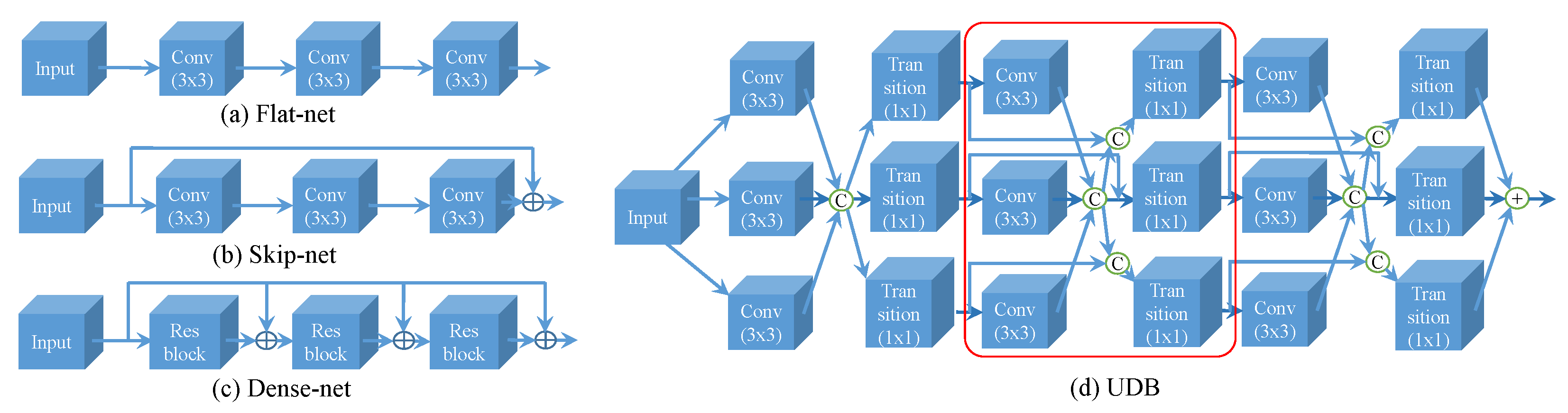
  • We propose a novel multiple-path residual block UDB, which provides additional possibilities for feature extraction through ultra-dense connections, quite agreeing with the uneven complexity of image content.
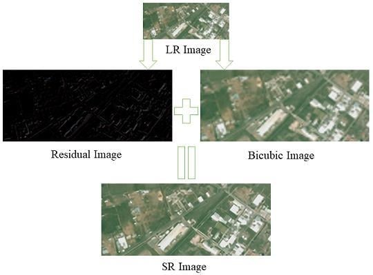
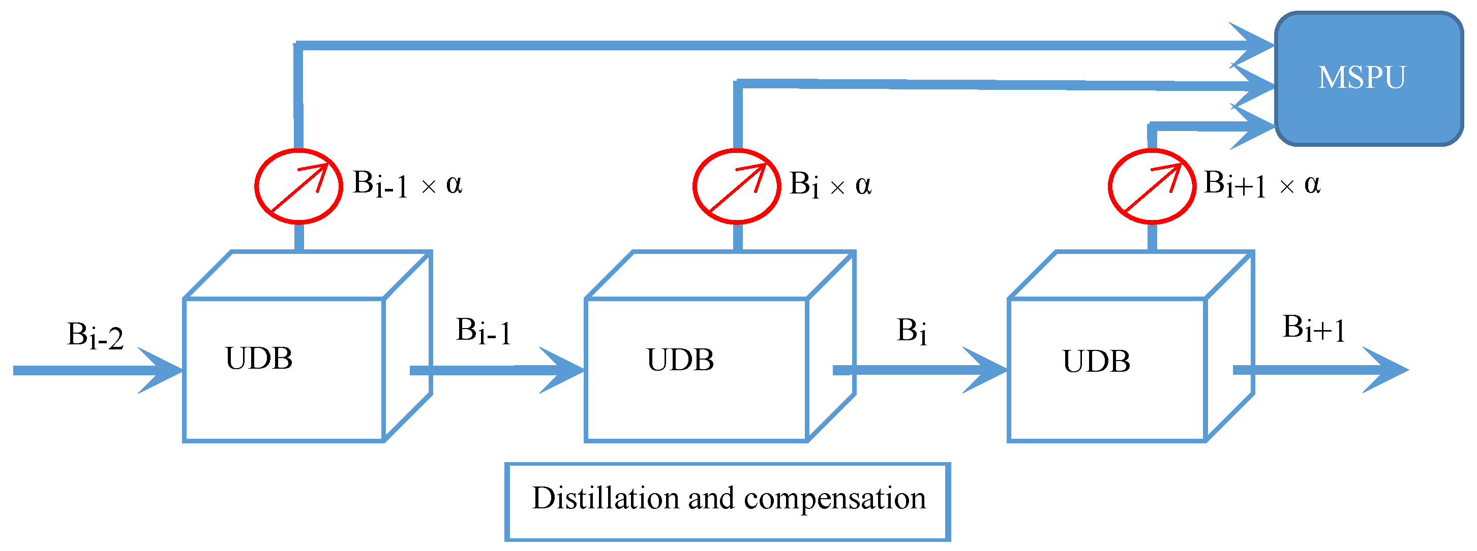
  • We construct a distillation and compensation mechanism to compensate for the high-frequency details lost during information propagation through the network with a special distillation ratio.
The remainder of this paper is organized as follows. In Section 2, we introduce previous works on CNN-based SR reconstruction algorithms, particularly network structures for feature extraction. Section 3 particularly presents the framework of the proposed DDRN. Section 4 individually presents the design of each key module under the proposed DDRN framework in details, including UDB, MSPU, resolution lifting, and loss function. Experimental results are given in Section 5, and the conclusions of this study are given in Section 6.

2. Related Work

We briefly review previously related works on structure-efficient networks [25,29,36,37,38], from which our network draws inspiration. These previous deep networks are committed to learning fine detail textures by designing a sophisticated structure. In this section, we focus on recent skip- and dense-connection-based methods.
Skip connection: A skip connection that directly connects input to output through an identity map, as shown in Figure 1b, was pioneered for SISR by Kim et al. [24]. They proposed a 20-layer CNN model known as VDSR. Instead of learning the actual pixel values, VDSR harnesses the global residual learning paradigm to predict the differences between ground truth and bicubic interpolated image. This learning strategy makes the feature maps very sparse, enabling easy training and convergence. Compared with the traditional methods [39,40,41,42], this learning strategy on the benchmark datasets shows a significant superiority on reconstruction performance in terms of visual and quantitative indicators. In addition, DRCN [29] constructes a recursive-supervision structure to alleviate the difficulty in training a deep residual network further. Recently, Sheng et al. [25] proposed a deep Laplacian pyramid super-resolution network (LapSRN) to reconstruct the sub-band residuals of HR images at multiple pyramid levels with skip connection.
Dense connection: Enlightened by previous works, Huang et al. [26] recently represented an intensive skip connection called dense connection. As shown in Figure 1c, the feature maps of the current layer are connected to every subsequent layer in a feed-forward manner. With rich local dense connections, the current layer can aggregate the information from all of the preceding layers within the dense block for further selection and fusion. These strategies effectively address the vanishing-gradient problem and enhance information propagation, thus strengthening the feature expression and boosting the convergence. Subsequently, Tong et al. [27] proposed an enhancement version called SRDenseNet. In SRDenseNet, the feature maps obtained from each dense block are propagated into the deconvolution layers to reconstruct SR images, providing an effective way to combine the low-level and high-level features, which further boosts the reconstruction performance. In addition, the dense skip connections in the network enable short paths to be built directly linking to the output from each layer, thus mitigating the vanishing-gradient problem. While considering the research on feature extraction and fusion, the earlier work of Gao et al. [38] is also noteworthy. They proposed a technique called multi-scale dense network for resource-efficient image classification. Their main idea is to train multiple classifiers in different stages using a two-dimensional multi-scale architecture, enabling them to preserve the coarse-and-fine level features all throughout the network.
Ultra-dense connection: These above mentioned strategies have been proven effective in addressing vanishing-gradient problem, guaranteeing accurate feature extraction and fusion. However, the directly concatenated operation on all layers in previous works [27,38] have led to high memory consumption and computation burden. In addition, conventional dense-connection-based networks have to construct a deeper network the more the skip paths required. Moreover, the increasing computational burden and memory consumption are unacceptable.
As shown in Figure 1d, on the basis of the dense network [26], we propose a multiple-path residual block called UDB. Compared with conventional skip or dense networks [24,26,27,29], UDB contains richer short and long paths with the same convolution layers. In particular, given the multiple-path units and transition layer, the feature channels becomes shallower, extremely reducing the parameters and decreasing the computational burden and memory consumption.

3. Network Architecture

As shown in Figure 2, the proposed model is a deep recursive neural network that can be roughly partitioned into three substructures, namely, local feature extraction and fusion, feature distillation, and feature compensation and SR reconstruction. Except for the upsampling operation, motivated by previous works on SISR [24,25,27,43], the entire process of local feature extraction and fusion is in the LR space. I L R and I S R are considered the LR input and HR output of the proposed DDRN, respectively. F i and B j refer to the output in the i t h layer and the j t h block, respectively. In this work, the LR RGB images are directly fed into the network and processed with the initial convolutional layers (two layers with 3 × 3 kernel) to extract features as follows:
F 1 = H ( I L R ) ,
F 2 = H ( F 1 ) ,
where H ( · ) denotes the convolution operation. F 1 and F 2 represent the shallow feature maps extracted through the initial convolutional layers, served as the input of the UDB. Moreover, the proposed residual block UDB is used as a basic module for local feature extraction in DDRN. For each UDB, the information cannot only be shared among layers and multiple-path units but also be used as the input for the subsequent residual blocks with ultra-dense connections. These strategies enforce information propagation and lead to fine feature expression by combining the multi-scale coarse-and-fine features in different stages. The operation can be defined as follows:
B i = H b l o c k , i ( B i 1 ) + B i 1 ,
where H b l o c k , i denotes the entire convolution operation in the i t h UDB and B i 1 refers to the extracted feature maps from the ( i 1 ) t h UDB. As shown in Figure 1, compared with the conventional CNN-based modules [24,25,26,29,30], whose commonly used residual block contains the simply direct or skip connections between layers, the proposed UDB module is composed of several interactive multiple-path units and parametric rectified linear units (PReLU). The dedicated architecture for UDB enjoys more linking paths in the same layers and provides more possibilities for feature extraction than do these previous strategies, thus matching the uneven content complexity of remote sensing imagery. Specifically, the simple links are adapted to smooth areas, whereas complex connections are suited for high-frequency texture details.
According to previous SISR algorithms [24,27,29,30], the output of the current stage is directly transmitted to the next stage. Then the final residual maps are obtained at the top layer for SR reconstruction. However, information loss is inevitable during its propagation in the network, thereby weakening the continuity of information propagation. Previous works add a set of nodes to shorten the transmission distance, thus boosting information propagation and reducing information loss during propagation, so-called skip connections [24,29]. However, increasing the nodes between the input and the output cannot only deepen the network but also increase computational burden and memory consumption. Differently, we facilitate information propagation with the multiple-path residual module UDB. Furthermore, we also present a distillation and compensation strategy for fine feature expression by compensating for extra-high-frequency details. As shown in Figure 3, unlike the traditional network, whose output in each block is directly transmitted to the subsequent part, our proposed method can adaptively distill and preserve the feature maps by partly choosing information from the current output yet retain its integrety. Then, these feature maps collected from different stages are aggregated and purified in MSPU to infer and compensate for the high-frequency details before the reconstruction operation.
In this study, we denote the preserved part from B i as the distillation unit ( D U ) with the ratio of α . At the same time, B i is used as the input to the subsequent residual block for further extraction. This process can be formulated as follows:
D U i = S ( B i , α ) ,
where α refers to the distillation ratio, which indicates that the feature maps in each stage with the ratio of α will be distilled and preserved. In our experiments, we set α to {0.0, 0.125, 0.25, 0.5}. S ( · ) represents the distillation operation, and D U i denotes the distilled information from the i t h residual block B i .
In addition, the reserved feature maps D U i in different stages are aggregated through a concatenation operation, and then they are fed into the purified unit MSPU, where the HR components lost in the previous blocks are reactivated as a compensation for SR reconstruction. In Equation (5), H C ( · ) denotes the concatenation operation adopted to collect the distillation information and M ( · ) refers to the MSPU. Through the distillation and compensation mechanism, the high-frequency components compensated from MSPU can further promote reconstruction performance.
P = M ( H C ( D U 0 , , D U i , , D U n ) ) ,
At the end of the network, the feature maps extracted from the top UDB and the compensated high-frequency details purified from MSPU are combined to infer and restore the HR components by a transition layer with 3 × 3 kernel. Then, a sub-pixel upsampling operation is used to project these features into HR space to obtain the residual image. The detailed operation is expressed as follows:
I S R = P S ( H S ( D n , P ) ) + I B ,
where D n and P represent the feature maps extracted from the top UDB and the compensated details from MSPU, respectively. H S denotes a transition function that contains a 3 × 3 convolution layer to fuse features and infer HR components, adaptively. I B refers to the bicubic interpolated image. P S ( · ) represents the reconstruction operation performing a sub-pixel amplification to obtain the HR residual image in the ending part of the network.

4. Feature Extraction and Distillation

In this section, we present the design of each key module under our DDRN framework in details, including UDB, MSPU, and Resolution Lifting.

4.1. Ultra-Dense Residual Block (UDB)

It is acknowledged that rich dense connections can promote feature expression [26,27]. Therefore, we design a dense connection module for feature extraction. In this study, a multiple-path residual block UDB is constructed to enforce the correlation among layers and blocks with rich dense connections. Compared with existing skip- or dense-connection-based methods, UDB considers diverse short and long linking paths (the multiple-path structure) and exhibits effective information-sharing capability among the layers. Therefore, our network provides additional possibilities for feature extraction, quite agreeing with the uneven complexity of image content. More precisely, simple links are adapted to smooth areas, whereas complex connections are suited for high-frequency texture details. As shown in Figure 1d, UDB includes several interactive multiple-path units, which can fuse the feature maps extracted from parallel multiple convolution paths. The information-sharing mechanism aggregates features in different levels to ensure a rich feature representation further. The function of the i t h unit can be formulated as follows:
y i = H C ( [ F i , 0 ( x 0 ) , F i , 1 ( x 1 ) , , F i , n ( x n ) ] ) ,
s i , n = H 1 ( H C ( y i , s i 1 , n ) ) .
Equations (7) and (8) formally show the operation process in a multiple-path unit. In Equation (7), F i , n ( x n ) and H C ( [ F i , 0 ( x 0 ) , F i , 1 ( x 1 ) , , F i , n ( x n ) ] ) refer to the single convolution operation and the feature congregation of multiple convolution layers in each unit, respectively. In Equation (8), y i denotes feature concatenation in the current unit. s i , n indicates the transition output in the n t h path of the i t h unit, and s i 1 , n represents the output from the n t h path of the ( i 1 ) t h unit. Functionally, a group of skip connections is used to enforce the correlation among the input and output feature maps, where the transition layers represented as H 1 are embedded to reduce feature channels with 1 × 1 convolution kernel.
Unlike skip- or dense-connection-based algorithms [26,27,28], the proposed multiple-path ultra-dense connection block can simultaneously explore and infer local and global features. In particular, the feature maps in the multiple-path unit cannot only be shared among the layers in the current unit through aggregation and dense connections but also be used as the input of other units with skip connections. Given the simplicity, effectiveness, and robustness of this strategy, local features can be well expressed through numerous short and long paths. Furthermore, owing to the effective structure for feature extraction in UDB, the network can become shallow in the channels but wide for the convolution paths, which extremely reduces the parameters and simultaneously boosts the reconstruction performance.

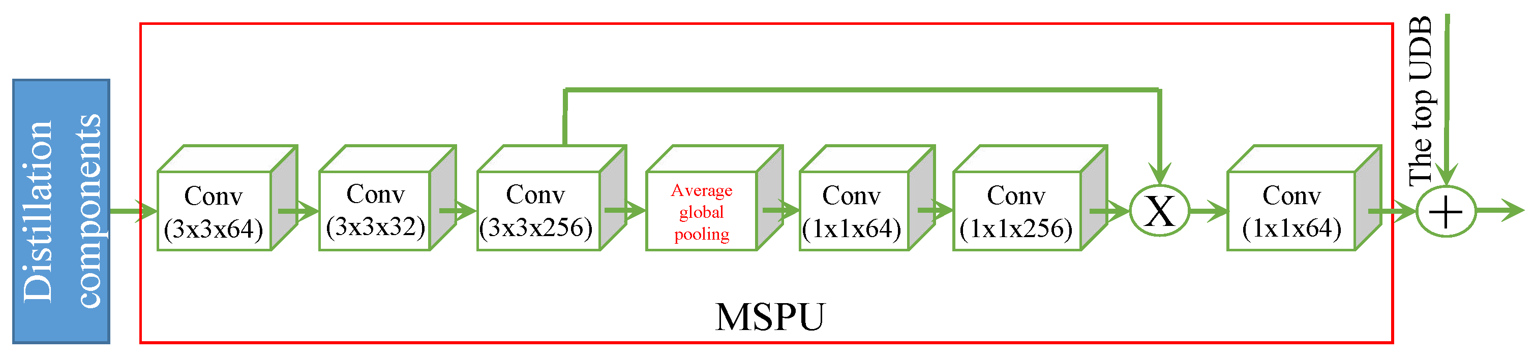
4.2. Multi-Scale Purification Unit (MSPU)

In [44], the authors focused on channels and proposed a novel architectural unit termed “squeeze-and-excitation” (SE) block to recalibrate channel-wise feature responses adaptively by explicitly modeling the interdependencies between channels. The SE block can learn to use global information to emphasise informative features and suppress less useful features selectively. This model won the first place in the classification contest I L S V R C 2017 [45].
In this study, we adopt the SE module because of its promising efficiency and efficacy. On the basis of this finding, we propose an applicable module MSPU for information compensation. The basic structure of MSPU building unit is illustrated in Figure 4. Contrary to the squeeze-and-excitation network (SEN) [44], the redundant residual connections between SE blocks used for features transmission are removed. In addition, given that the full connection layer can destroy the internal structure of the image, we therefore replace it with a 1 × 1 convolution layer. Moreover, we adopt a robust activation function, e.g., parametric rectified linear unit (PReLU), to replace the previous version rectified linear unit (ReLU).
On the basis of MSPU process, we further propose a distillation and compensation strategy to compensate for lost details. By partially distilling the components from B i with the distillation ratio of α , as shown in Figure 3, we can obtain feature maps originating from UDB in different stages. Then, these features are aggregated into MSPU to purify and gain more abundant and efficient information. The extraction functions can be defined as follows:
M S = H ( x ) ,
P = σ ( H 1 ( A P ( M S ) ) ) × M S .
In Equation (9), the input x denotes the concatenation of the distilled components in different satges, equivalent to H C ( D U 0 , , D U i , , D U n ) in Equation (5), and H ( · ) represents a group of convolutional operations (with 3 × 3 kernel) that is adopted to fuse the features distilled from different levels. As expressed in Equation (10), A P denotes the global average pooling, H 1 refers to the group of transition layers that comprises the bottleneck structure, and σ represents the sigmoid function.

4.3. Resolution Lifting

To project a single LR image into HR space, the resolution of LR image must be increased to match that of the HR image at a certain point. Osendorfer et al. [46] presented a computationally efficient architecture for image SR by leveraging the fast approximate inference to increase the image resolution in the middle of the network gradually. Another well-known approach can also achieve spatial resolution enhancement by linear interpolation [23,24]. They obtained the same image resolution by directly using the common bicubic interpolation before loading the dataset into the network.
In addition, the early work of Shi et al. [47] is noteworthy when considering the upsampling operation. Contrary to authors of previous works, the researchers proposed an efficient sub-pixel convolution layer to increase the image resolution only at the final layer, eliminating the need to perform most of the SR operations in the large HR space. Compared with the transposed convolution and bicubic interpolation, sub-pixel magnification [47] is actually a realignment of feature maps without extra parameters, thus quite decreasing memory consumption and computational cost. These reasons enable the network go deeper and be trained easily.
As expressed in Equation (11), P S is a shuffling operator that rearranges the elements of a H × W × C · r 2 tensor acquired in the top layer into a r H × r W × C tensor (where r is the magnification factor of the network, and C refers to the feature channels of the input image). Mathematically, the upsampling function can be expressed as follows:
P S ( T ) x , y , c = T x / r , y / r ( mod ( x , r ) , mod ( y , r ) ) ,
where T indicates the output from the final layer with the size of W × H × C r 2 , ( x , y ) denotes the output pixel coordinate in the HR space, ( x / r , y / r ) represents the pixel area of r × r in the sub-pixel space, and ( mod ( x , r ) , mod ( y , r ) ) refers to the pixel coordinate in LR space. The C r 2 channels of each pixel in the same location in the LR space is rearranged into a region of 1 r × 1 r × C , which corresponds to a subblock in an HR image, and the feature image is rearranged into an HR image of r W × r H × C .
In this work, as in many CNN-based SISR methods [25,47,48], we adopt the sub-pixel upsampling strategy to reconstruct the HR image at the top layer because of its promising efficiency and efficacy.

4.4. Loss Function

It is well known that SISR is an ill-posed problem whose solution from the reconstruction constraint is not unique because of the insufficient number of LR images, ill-conditioned registration, and unknown degradation process. In previous works, the loss function is commonly used to fit the real target image by minimizing the distance between the reconstructed HR image and the ground truth. The commonly used distance measurements include pixel-based l 1 -norm [25] and l 2 -norm [23,24,29], and cosine distance based on feature level.
Most of the previous works [23,27,29] constrain the reconstruction image by minimizing the mean squared error (MSE) or maximizing the peak signal to noise ratio (PSNR), which is a common measure used to evaluate SR algorithms [49]. However, the capability of MSE to capture perceptually relevant components, such as high-frequency texture details, is insufficient because they are defined on basis of pixel-wise image differences [50]. For example, the previous works [23,29,43] use MSE loss as the cost function and produce overly smooth reconstruction results that are inconsistent with human vision. In [25,51], the authors proposed a novel optimal function charbonnier loss based on the l 1 -norm, which can recover a large amount of realistic details, more faithful to the ground truth. In our work, we therefore introduce the charbonnier penalty function to penalize the deviation of the prediction from the residuals of ground truth. The loss function can be expressed as follows:
L o s s ( I S R , I H R , θ ) = arg min θ ρ ( I H R f ( I L R , θ ) ) ,
where θ denotes a set of model parameters to be optimized and ρ ( x ) = x 2 + ε 2 represents the charbonnier penalty function (a differentiable variant of l 1 -norm). We empirically set the compensation parameter ε of 10−3. I S R and I H R refer to the predicted HR image and the ground truth.

5. Experimental Results and Analysis

In this section, first, we describe the experimental settings, including the data collection and model parameters. Then, we assess the effect of the distillation ratio α and the network depth m on the reconstruction performance. Subsequently, we compare our results with these state-of-the-art techniques and provide a thorough analysis. We retrain the comparison algorithms with our training dataset to ensure a fair comparison, including SRCNN [23] and VDSR [24]. Moreover, we directly apply the original models [23,24,25] trained with general image datasets, as the anchors.

5.1. Data Collection

For general image SR, a large quantity of public training and assessing datasets, such as DIV2K [52], BSD500 [53] and Yang291 [39], are used to evaluate the results. However, few available datasets can be used as the training samples for satellite imagery SR because of the special requirements of ground target resolution. We use two available satellite image datasets, namely, Kaggle Open Source Dataset and Jilin-1 video satellite imagery, to train and evaluate the proposed DDRN method.
  • The first imagery dataset is the Kaggle Open Source Dataset (https://www.kaggle.com/c/draper-satellite-image-chronology/data), which contains more than 1000 HR images of aerial photographs captured in southern California. The photographs were taken from a plane and meant as a reasonable facsimile for satellite images. The images are grouped into five sets, each of which having the same setId. Each scenario in a set contains five images captured on different days (not necessarily at the same time each day). The images for each set cover approximately the same area but are not exactly aligned. Images are named according to the convention (setId-day). In this dataset, the scene has 3099 × 2329 pixels and 324 different scenarios. A total of 1720 satellite images cover agriculture, airplane, buildings, golf course, forest, freeway, parking lot, tennis court, storage tanks, and harbor. In this study, 30 different categories are selected for the test and 10 for the evaluation. Meanwhile, a total of 350 images are used for the training. Regarding the training dataset, the entire images are cropped into many batches with 720 × 720 pixels, but only the central area of the testing images with size of 720 × 720 pixels is cropped for testing and evaluation.
  • The second satellite dataset is from Jilin-1 video satellite imagery. In 2015, the Changchun Institute of Optics, Fine Mechanics, and Physics successfully launched the Jilin-1 video satellite which had 1.12 m resolution. To cover the duration of video sequences, we select one for every five frames from each video and crop the central part with the size of 480 × 204 as test samples. We select several areas in different countries with certain typical surface coverage types, including vegetation, harbor, and a variety of buildings as the test images.

5.2. Model Parameters and Experiment Setup

In our experiments, we use an NVIDIA GTX1080Ti GPU and an Intel I7-8700K CPU for training and testing, respectively. Our model is implemented on TensorFlow with Python3 under Windows10, CUDA8.0, and CUDNN5.1 systems. We mainly focus on the up-scaling factor of 4, which is usually the most challenging case in image SR.
The original HR images are downsized by bicubic interpolation to generate LR images for training. We augment the training patches by horizontal or vertical flipping and rotating 90. By following the settings presented in [54], we send one batch consisting of 16 LR RGB patches with the size of 32 × 32 from the training datasets to our network each time. The learning rate is initialized to 10−3 for all layers and halved for every 104 steps up to 10−5. In our model, each convolution layer contains 64 filters, followed by PReLU. We empirically set the distillation ratio α to {0.0, 0.125, 0.25, 0.5} and the number of parallel convolution layers n in each multiple-path unit to 3. For the basic module DDRN, the depth of UDB is 15. In our experiments, training a basic module consumes approximately 20 h under the previously presented experimental settings.

5.3. Quantitative Indicators (QI)

Similar to many previous representative works [23,24,28,29], we also select two commonly used evaluation metrics, i.e., PSNR and structural similarity (SSIM), to evaluate the model performance. These evaluation metrics differ in terms of visual perception but involve reference images for comparison. However, in real SR scenes, we have only LR images to be super-resolved, without the corresponding HR reference image.Therefore, we need to introduce quantitative non-reference image quality assessment methods. Quality with no reference (QNR) [55,56], generalized quality with no reference (GQNR) [57] and average gradient (AG) [58] are commonly used image quality evaluation algorithms without reference, which can reasonably assess the clarity of reconstructed image. Nevertheless, QNR and GQNR are used for multispectral or hyperspectral images rather than ordinary RGB images, which needs to calculate the spectral distortion index and spatial distortion index. Thus, in this study, we propose to alternatively use AG for objective evaluation without reference. This process can be expressed as follows:
G ( x , y ) = d x ( i , j ) + d y ( i , j ) ,
d x ( i , j ) = I ( i + 1 , j ) I ( i , j ) ,
d y ( i , j ) = I ( i , j + 1 ) I ( i , j ) ,
where d x and d y refer to the horizontal and vertical gradients, respectively, and I ( i , j ) denotes the pixel value corresponding to the coordinate of ( i , j ) .
The indicator of the AG can reasonably assess image clarity because it sensitively reflects content sharpness, detail contrast, and texture diversity. Generally, the larger the AG, the richer the details. Thus, the AG can be used to evaluate the reconstruction quality of satellite imagery in real-world scenes, such as Jilin-1 video satellite imageries.

5.4. Validation of the Ultra-Dense Residual Block

We examine the effectiveness of the proposed deep recursive CNN network DDRN and the multiple-path UDB. Given that SRCNN [23] and VDSR [24] are the most representative and most effective deep-learning-based SR methods, in our experiments, we retrain these two models by using the same training datasets and label them as SRCNN* and VDSR*. Figure 5 shows the comparison results according to the iterations of DDRN, SRCNN, and VDSR. Comparatively, our DDRN exhibits faster convergence and higher scores than do direct-connection-based SRCNN and skip-connection-based VDSR. This superiority can be mainly attributed to the proposed multiple-path ultra-dense connections which can readily capture local features. Thus, our framework significantly boosts the SR efficacy of remote sensing imagery.
In Figure 6, we show the evaluation results of the proposed DDRN method and the comparison algorithms on the Kaggle Open Source Dataset to verify the usefulness of the ultra-dense connections strategy further. The test set contains 30 different scenarios, which are labeled 1 to 30 in Figure 6. The figure shows that by using ultra-dense connections, we obtain better reconstruction results than do the conventional CNN-based methods, i.e., SRCNN [23] and VDSR [24]. For the average PSNR, our DDRN shows substantial improvements, surpassing VDSR by 0.92 dB, and SRCNN by 1.94 dB. Similarly, SSIM is also considerably improved.
In summary, the proposed residual block UDB effectively captures realistic detail textures. Although SRCNN and VDSR are effective, the well-designed deep recursive framework DDRN is more suitable for satellite image SR reconstruction.

5.5. Influence of Parameters α and m

On the basis of the basic module DDRN, we implement a distillation and compensation mechanism to compensate for the HR components lost during information propagation to infer and restore more realistic high-frequency details. The improved model with MSPU embedment is called DDRN+. In particular, a couple of comparison simulation experiments are conducted to analyze the influences of (i) the hyperparameter α in Equation (4) for partial feature maps distillation and preservation, (ii) the depth value m of UDB on the reconstruction performance.
We report the training process of the proposed DDRN+ with respect to different distillation ratios to verify the necessity of the proposed distillation and compensation mechanism. When α is set to 0, no components are distilled in the current stage, whereas MSPU does not function. Figure 7 shows the comparison results of the training process under different distillation ratios. From the figure, we learn that the proposed DDRN+ exhibits better training performance than the basic module DDRN. In addition, we observe that, with an increase in the distillation ratio α , the module exhibits robust and fast convergence. This result can be attributed to the increasing compensated high-frequency details from the MSPU by an increased distillation ratio. However, we also observe that the performance starts to decline when α is set to a large value, e.g., 0.5. This result can be mainly attributed to the large distillation rate, which may result in information redundancy. In addition, excessive parameters might lead to overfitting. All of these results indicate that the proposed distillation and compensation mechanism show substantial improvements by compensating for high-frequency details. Therefore, embedding MSPU into the basic module for satellite image SR reconstruction is an effective and reliable choice.
In light of the observations in these previous works [26,27,28], fine features can be well inferred from a deep CNN framework. Thus, we gradually increase the depth of the network by simply adding the number of the UDB (i.e., m is set to 10, 15, 20, 25, 30, and 35). We assess the performance of different values of m. In Figure 8, we show the training details of the proposed DDRN+ method with different depths. When simply increasing the value of m to 30, the improvement gradually increases and surpasses the basic module by approximately 0.22 dB in the scale of 4. By contrast, the performance declines when we continue to increase m to 35 and the network exhibits slow convergence. This result can be mainly attributed to the overfitting, and the convergence of the network becomes more difficult in such a depth.
On the basis of the experiments, we can obtain the optimal distillation ratio α and UDB depth m for satellite image SR reconstruction, which are set to 0.25 and 30, respectively.

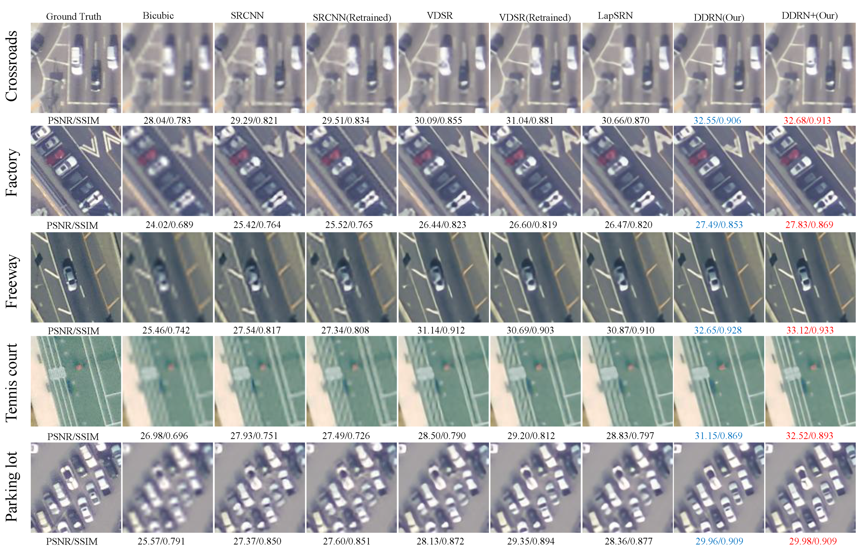
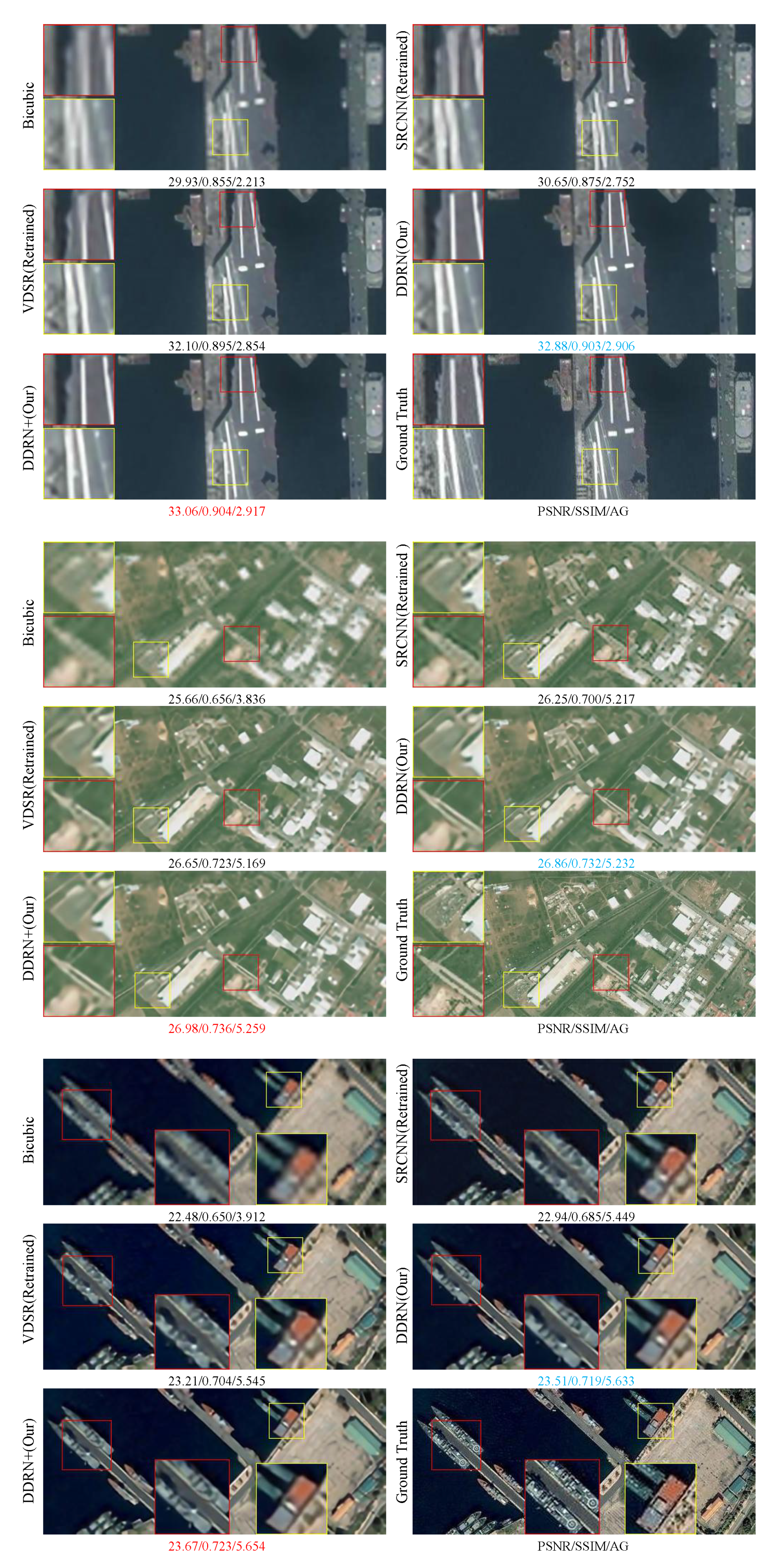
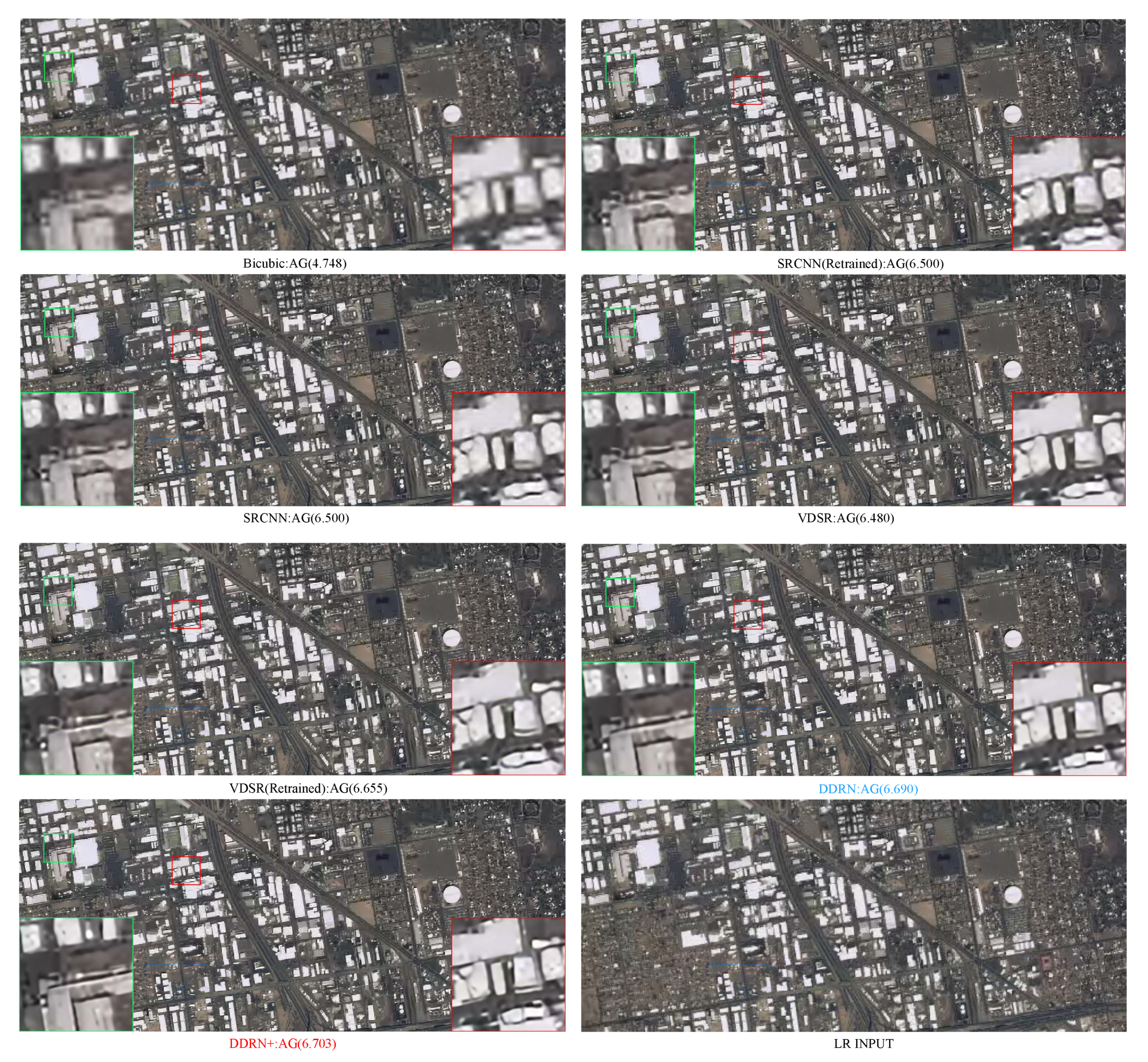
5.6. Comparison Results with the State-of-the-Art

We compare our basic model DDRN and the improved version DDRN+ ( α = 0.25 , m = 30 ) with other SISR algorithms, including Bicubic, SRCNN [23], VDSR [24], and LapSRN [25], by the scaling factors of ×2, ×3, and ×4. The implementations of these anchor methods have been released online and can thus be conducted on the same test datasets.
The reconstruction results obtained with above mentioned Kaggle Open Source Dataset for the proposed approaches and the comparison methods are shown in Figure 9. We select several different but representative scenarios (i.e., crossroads, factory, freeway, tennis court, and parking lot) to produce a visual presentation. Experimentally, we crop these representative scenarios into a sub-batch with the size of 120 × 120 pixels from each reconstructed SR image and compute PSNR and SSIM. Notably, the proposed method DDRN and its improved version DDRN+ surpass these state-of-the-art methods by a large margin. Moreover, the modules that we propose exhibit the most accurate and realistic image details from the visual effect. Most of the comparison methods produce noticeable artifacts and blurred edges, whereas the proposed DDRN+ can recover sharper and clearer edges because of successful feature extraction and fusion, more faithful to the ground truth. For example, as shown in Figure 9, only our proposed modules restore the clear court boundary in the tennis court scenario and the accurate and credible car outline in the four other scenarios. Therefore, all of the proposed models exhibit solid performance improvements compared with the conventional direct- or skip-connection-based algorithms [23,24,25].
Objectively, Table 1, Table 2 and Table 3 tabulate the detailed evaluating results in terms of PSNR, SSIM and AG with the magnification scales of ×2, ×3, and ×4, respectively. From these records, we learn that raw CNN-based or skip connection methods, such as SRCNN [23] and VDSR [24], exhibit lower scores than do DDRN-based methods (i.e., in terms of PSNR, the proposed DDRN+ surpasses SRCNN and VDSR retrained by approximately 2.16 and 1.14 dB with the scale of 4 in the first test dataset, respectively.). Among these comparison methods, the basic module DDRN shows the best performances because of its ultra-dense-connection-based effective framework for local spatial information extraction. In addition, through the compensated high-frequency details obtained from the MSPU, the improved version DDRN+ can produce fine detail textures. With regard to PSNR and SSIM, Figure 6 shows an more intuitive result that the proposed modules outperform these state-of-the-art methods [23,24,25] by a large margin. For the metric AG, the proposed DDRN and DDRN+ are also better than previous works on average. In particular, in the comparison results shown in the three tables, our methods exhibit remarkable advantages when the upsampling factor is large, as reported at the bottom of the three tables. These results indicate the advantages of the proposed ultra-dense-connection manner in modeling the relationship between LR and HR images with lager magnification factors.
Another group of comparison experiments are conducted with the Jilin-1 satellite imagery to illustrate the effectiveness and applicability of the proposed ultra-dense strategy and distillation and compensation mechanism further. Compared with the first dataset Kaggle Open Source Dataset, the test images obtained from Jilin-1 show lower quality (small ground objects and weak textures) but more realistic satellite imagery characteristics. Unlike the images in the training dataset, the test images have completely different imaging conditions, including ultra-high imaging distance, atmospheric scattering, relative motion between satellite and moving ground targets, and compression distortion. These severe imaging conditions pose substantial demands to SR networks.
With an operation similar to the previously presented preprocessing of the testing images, we crop the test images with the size of 480 × 204. The reconstruction results obtained from our proposed approaches and the comparison methods are shown in Figure 10. For the first and second images, most of the comparison methods produce noticeable artifacts and blurred edges. By contrast, the proposed DDRN and DDRN+ can recover sharp and clear edges because of fine feature expression that is faithful to the ground truth. At the bottom of the figure, only our proposed modules can reconstruct a clear outline of the warships and dock, whereas the other conventional methods fail to restore the realistic details. These results further indicate the effectiveness of the proposed method.
Furthermore, we perform a set of realistic SR reconstruction experiments for the unknown real degradation process (i.e., using the observed LR images instead of the downscaled LR images as input). These test images are randomly selected from Jilin-1 satellite imagery using the same preprocessing to acquire the test images with the size of 480 × 204. Then, the processed images used as the LR input are directly transmitted to the network to obtain the reconstructed HR images. The comparison results with other state-of-the-art algorithms are shown in Figure 11 (we show only one example due to space constrains). Evidently, most of compared methods [23,24] produce noticeable artifacts and blurred building outlines, whereas the proposed DDRN and DDRN+ yield better results with fewer jagged lines and ringing artifacts. Instead of the commonly used evaluation metrics PSNR and SSIM (because the original HR images are unavailable), we introduce the AG to measure the sharpness of the SR results. As shown in Figure 11, the proposed modules DDRN and DDRN+ enjoy the second and first highest AG scores, respectively. The results for real video satellite imagery indicate that our model is more robust than the comparison methods in super-resolving the image with unknown degradation process.
In brief, the SR reconstruction experiments on different test datasets and magnification scales show the advantages of feature expression and indicate the robustness of our modules against images of unknown degradation models.

6. Conclusions

In this study, we propose a simple but very effective technique for remote sensing image SR reconstruction. In particular, we present a multiple-path UDB for local feature extraction and fusion. Unlike in the conventional methods, rich dense connections between layers and units promote information interaction and improve reutilization. In addition, we further promote feature expression by advocating a distillation and compensation mechanism. The feature maps distilled from different stages with a special distillation ratio α are aggregated to compensate for the high-frequency details lost during information propagation in MSPU. Extensive experiments on the test datasets indicate that the proposed DDRN and its improved version DDRN+ outperform existing state-of-the-art feature extraction techniques, including conventional direct- and skip-connection-based methods. In particular, when the image degradation model is unknown, the proposed algorithm can still obtain competitive reconstruction results compared with the comparison algorithms.

Author Contributions

Conceptualization, K.J. and Z.W.; Data curation, K.J. and P.Y.; Formal analysis, P.Y. and J.J.; Funding acquisition, Z.W.; Investigation, J.X.; Methodology, K.J. and Z.W.; Project administration, K.J.; Resources, Z.W.; Software, P.Y.; Supervision, Y.Y.; Validation, K.J., Z.W. and J.J.; Visualization, P.Y.; Draft Preparation, K.J.; Writing, review and editing, Z.W. and J.J.

Funding

This research was funded by [National Natural Science Foundation of China] grant number [61671332, 41771452, 41771454, 61501413], [National Key R&D Project] grant number [2016YFE0202300], and [Hubei Province Technological Innovation Major Project] grant number [2017AAA123]. (Corresponding author: Zhongyuan Wang).

Conflicts of Interest

The authors declare no conflict of interest.

Abbreviations

The following abbreviations are used in this manuscript:
CNNsConvolutional neural networks
SRSuper-resolution
SISRSingle image super-resolution
LRLow resolution
HRHigh resolution
DDRNDeep distillation recursive network
UDBUltra-dense residual block
MSPUMulti-scale purification unit

References

  1. Xu, Y.; Zhu, M.; Li, S.; Feng, H.; Ma, S.; Che, J. End-to-end airport detection in remote sensing images combining cascade region proposal networks and multi-threshold detection networks. Remote Sens. 2018, 10, 1516. [Google Scholar] [CrossRef]
  2. Shao, Z.; Wu, W.; Wang, Z.; Du, W.; Li, C. SeaShips: A large-scale precisely annotated dataset for ship detection. IEEE Trans. Multimed. 2018, 20, 2593–2604. [Google Scholar] [CrossRef]
  3. Ma, J.; Zhao, J.; Tian, J.; Yuille, A.L.; Tu, Z. Robust point matching via vector field consensus. IEEE Trans. Image Process. 2014, 23, 1706–1721. [Google Scholar]
  4. Ma, J.; Jiang, J.; Zhou, H.; Zhao, J.; Guo, X. Guided locality preserving feature matching for remote sensing image registration. IEEE Trans. Geosci. Remote Sens. 2018, 56, 4435–4447. [Google Scholar] [CrossRef]
  5. Jiang, J.; Ma, J.; Chen, C.; Wang, Z.; Cai, Z.; Wang, L. SuperPCA: A superpixelwise PCA approach for unsupervised feature extraction of hyperspectral imagery. IEEE Trans. Geosci. Remote Sens. 2018, 56, 4581–4593. [Google Scholar] [CrossRef]
  6. Jiang, J.; Ma, J.; Wang, Z.; Chen, C.; Liu, X. Hyperspectral image classification in the presence of noisy labels. IEEE Trans. Geosci. Remote Sens. 2018. [Google Scholar] [CrossRef]
  7. Li, C.; Ma, Y.; Mei, X.; Liu, C.; Ma, J. Hyperspectral unmixing with robust collaborative sparse regression. Remote Sens. 2016, 8, 588. [Google Scholar] [CrossRef]
  8. Ma, J.; Ma, Y.; Li, C. Infrared and visible image fusion methods and applications: A survey. Inf. Fus. 2019, 45, 153–178. [Google Scholar] [CrossRef]
  9. Ma, J.; Yu, W.; Liang, P.; Li, C.; Jiang, J. FusionGAN: A generative adversarial network for infrared and visible image fusion. Inf. Fus. 2019, 48, 11–26. [Google Scholar] [CrossRef]
  10. Dong, W.; Fu, F.; Shi, G.; Cao, X.; Wu, J.; Li, G.; Li, X. Hyperspectral image super-resolution via non-negative structured sparse representation. IEEE Trans. Image Process. 2016, 25, 2337–2352. [Google Scholar] [CrossRef] [PubMed]
  11. Yang, S.; Sun, F.; Wang, M.; Liu, Z.; Jiao, L. Novel super resolution restoration of remote sensing images based on compressive sensing and example patches-aided dictionary learning. In Proceedings of the International Workshop on Multi-Platform/Multi-Sensor Remote Sensing and Mapping, Xiamen, China, 10–12 January 2011; pp. 1–6. [Google Scholar]
  12. Jiang, K.; Wang, Z.; Yi, P.; Jiang, J. A progressively enhanced network for video satellite imagery superresolution. IEEE Signal Process. Lett. 2018, 25, 1630–1634. [Google Scholar] [CrossRef]
  13. Luo, Y.; Zhou, L.; Wang, S.; Wang, Z. Video satellite imagery super resolution via convolutional neural networks. IEEE Geosci. Remote Sens. Lett. 2017, 14, 2398–2402. [Google Scholar] [CrossRef]
  14. Xiao, A.; Wang, Z.; Wang, L.; Ren, Y. Super-resolution for “Jilin-1” satellite video imagery via a convolutional network. Sensors 2018, 18, 1194. [Google Scholar] [CrossRef] [PubMed]
  15. Merino, M.T.; Nunez, J. Super-resolution of remotely sensed images with variable-pixel linear reconstruction. IEEE Trans. Geosci. Remote Sens. 2007, 45, 1446–1457. [Google Scholar] [CrossRef] [Green Version]
  16. Li, F.; Jia, X.; Fraser, D. Universal HMT based super resolution for remote sensing images. In Proceedings of the 15th IEEE Conference on ICIP, San Diego, CA, USA, 12–15 October 2008; pp. 333–336. [Google Scholar]
  17. Gou, S.; Liu, S.; Yang, S.; Jiao, L. Remote sensing image super-resolution reconstruction based on nonlocal pairwise dictionaries and double regularization. IEEE J. Sel. Top. Appl. Earth Observ. 2014, 7, 4784–4792. [Google Scholar] [CrossRef]
  18. Li, Y.; Zhang, Y.; Huang, X.; Zhu, H.; Ma, J. Large-scale remote sensing image retrieval by deep hashing neural networks. IEEE Trans. Geosci. Remote Sens. 2018, 56, 950–965. [Google Scholar] [CrossRef]
  19. Shao, Z.; Cai, J. Remote sensing image fusion with deep convolutional neural network. IEEE J. Sel. Top. Appl. Earth Observ. 2018, 11, 1656–1669. [Google Scholar] [CrossRef]
  20. Zhou, W.; Newsam, S.; Li, C.; Shao, Z. Learning low dimensional convolutional neural networks for high-resolution remote sensing image retrieval. Remote Sens. 2017, 9, 489. [Google Scholar] [CrossRef]
  21. Lu, T.; Ming, D.; Lin, X.; Hong, Z.; Bai, X.; Fang, J. Detecting building edges from high spatial resolution remote sensing imagery using richer convolution features network. Remote Sens. 2018, 10, 1496. [Google Scholar] [CrossRef]
  22. Zhang, W.; Witharana, C.; Liljedahl, A.K.; Kanevskiy, M. Deep convolutional neural networks for automated characterization of arctic ice-wedge polygons in very high spatial resolution aerial imagery. Remote Sens. 2018, 10, 1487. [Google Scholar] [CrossRef]
  23. Dong, C.; Loy, C.C.; He, K.; Tang, X. Image super-resolution using deep convolutional networks. IEEE Trans. Pattern Anal. Mach. Intell. 2016, 38, 295–307. [Google Scholar] [CrossRef] [PubMed]
  24. Kim, J.; Lee, J.K.; Lee, K.M. Accurate image super-resolution using very deep convolutional networks. In Proceedings of the IEEE Conference on CVPR, Las Vegas, NV, USA, 27–30 June 2016; pp. 1646–1654. [Google Scholar]
  25. Lai, W.S.; Huang, J.B.; Ahuja, N.; Yang, M.H. Deep laplacian pyramid networks for fast and accurate super-resolution. In Proceedings of the IEEE Conference on CVPR, Honolulu, HI, USA, 21–26 July 2017; pp. 5835–5843. [Google Scholar]
  26. Huang, G.; Liu, Z.; van der Maaten, L.; Weinberger, K.Q. Densely connected convolutional networks. In Proceedings of the IEEE Conference on CVPR, Honolulu, HI, USA, 21–26 July 2017; pp. 2261–2269. [Google Scholar]
  27. Tong, T.; Li, G.; Liu, X.; Gao, Q. Image super-resolution using dense skip connections. In Proceedings of the IEEE Conference on ICCV, Venice, Italy, 22–29 October 2017; pp. 4809–4817. [Google Scholar]
  28. Tai, Y.; Yang, J.; Liu, X.; Xu, C. MemNet: A persistent memory network for image restoration. In Proceedings of the IEEE Conference on ICCV, Venice, Italy, 22–29 October 2017; pp. 4549–4557. [Google Scholar]
  29. Kim, J.; Lee, J.K.; Lee, K.M. Deeply-recursive convolutional network for image super-resolution. In Proceedings of the IEEE Conference on CVPR, Las Vegas, NV, USA, 27–30 June 2016; pp. 1637–1645. [Google Scholar]
  30. Tai, Y.; Yang, J.; Liu, X. Image super-resolution via deep recursive residual network. In Proceedings of the IEEE Conference on CVPR, Honolulu, HI, USA, 21–26 July 2017; pp. 2790–2798. [Google Scholar]
  31. Yang, W.; Feng, J.; Yang, J.; Zhao, F.; Liu, J.; Guo, Z.; Yan, S. Deep edge guided recurrent residual learning for image super-resolution. IEEE Trans. Image Process. 2017, 26, 5895–5907. [Google Scholar] [CrossRef] [PubMed]
  32. Yim, J.; Joo, D.; Bae, J.; Kim, J. A gift from knowledge distillation: Fast optimization, network minimization and transfer learning. In Proceedings of the IEEE Conference on CVPR, Honolulu, HI, USA, 21–26 July 2017; pp. 7130–7138. [Google Scholar]
  33. Gupta, S.; Hoffman, J.; Malik, J. Cross modal distillation for supervision transfer. In Proceedings of the IEEE Conference on CVPR, Las Vegas, NV, USA, 27–30 June 2016; pp. 2827–2836. [Google Scholar]
  34. Hinton, G.; Vinyals, O.; Dean, J. Distilling the knowledge in a neural network. Comput. Sci. 2015, 14, 38–39. [Google Scholar]
  35. Pintea, S.L.; Liu, Y.; van Gemert, J.C. Recurrent knowledge distillation. In Proceedings of the 25th IEEE Conference on ICIP, Athens, Greece, 7–10 October 2018; pp. 3393–3397. [Google Scholar]
  36. Zhao, P.; Liu, K.; Zou, H.; Zhen, X. Multi-stream convolutional neural network for SAR automatic target recognition. Remote Sens. 2018, 10, 1473. [Google Scholar] [CrossRef]
  37. Gu, S.; Zuo, W.; Xie, Q.; Meng, D.; Feng, X.; Zhang, L. Convolutional sparse coding for image super-resolution. In Proceedings of the IEEE Conference on ICCV, Santiago, Chile, 7–13 December 2015; pp. 1823–1831. [Google Scholar]
  38. Huang, G.; Chen, D.; Li, T.; Wu, F.; van der Maaten, L.; Weinberger, K.Q. Multi-scale dense networks for resource efficient image classification. arXiv, 2018; arXiv:1703.09844. [Google Scholar]
  39. Yang, J.; Wright, J.; Huang, T.S.; Ma, Y. Image super-resolution via sparse representation. IEEE Trans. Image Process. 2010, 19, 2861–2873. [Google Scholar] [CrossRef] [PubMed]
  40. Timofte, R.; De, V.; Gool, L.V. Anchored neighborhood regression for fast example-based super-resolution. In Proceedings of the IEEE Conference on ICCV, Sydney, Australia, 8 April 2013; pp. 1920–1927. [Google Scholar]
  41. Yang, J.; Wright, J.; Huang, T.; Ma, Y. Image super-resolution as sparse representation of raw image patches. In Proceedings of the IEEE Conference on CVPR, Anchorage, Alaska, 23–28 June 2008; pp. 1–8. [Google Scholar]
  42. Yang, C.Y.; Yang, M.H. Fast direct super-resolution by simple functions. In Proceedings of the IEEE Conference on ICCV, Sydney Australia, 8 April 2013; pp. 561–568. [Google Scholar]
  43. Dong, C.; Chen, C.L.; Tang, X. Accelerating the super-resolution convolutional neural network. In Proceedings of the IEEE Conference on ECCV, Amsterdam, The Netherlands, 8–16 October 2016; pp. 391–407. [Google Scholar]
  44. Hu, J.; Shen, L.; Sun, G. Squeeze-and-excitation networks. arXiv, 2018; arXiv:1709.0150. [Google Scholar]
  45. Russakovsky, O.; Deng, J.; Su, H.; Krause, J.; Satheesh, S.; Ma, S.; Huang, Z.; Karpathy, A.; Khosla, A.; Bernstein, M.; et al. ImageNet large scale visual recognition challenge. Int. J. Comput. Vis. 2015, 115, 211–252. [Google Scholar] [CrossRef]
  46. Osendorfer, C.; Soyer, H.; Smagt, P.V.D. Image super-resolution with fast approximate convolutional sparse coding. In Proceedings of the International Conference on Neural Information Processing, Kuching, Malaysia, 3–6 November 2014; pp. 250–257. [Google Scholar]
  47. Shi, W.; Caballero, J.; Huszár, F.; Totz, J.; Aitken, A.P.; Bishop, R.; Rueckert, D.; Wang, Z. Real-time single image and video super-resolution using an efficient sub-pixel convolutional neural network. In Proceedings of the IEEE Conference on CVPR, Las Vegas, NV, USA, 27–30 June 2016; pp. 1874–1883. [Google Scholar]
  48. Lim, B.; Son, S.; Kim, H.; Nah, S.; Lee, K.M. Enhanced deep residual networks for single image super-resolution. In Proceedings of the IEEE Conference on CVPRW, Honolulu, HI, USA, 21–26 July 2017; pp. 1132–1140. [Google Scholar]
  49. Yang, C.Y.; Ma, C.; Yang, M.H. Single-image super-resolution: A nenchmark. Lect. Notes Comput. Sci. 2014, 8692, 372–386. [Google Scholar]
  50. Wang, Z.; Bovik, A.C.; Sheikh, H.R.; Simoncelli, E.P. Image quality assessment: from error visibility to structural similarity. IEEE Trans. Image Process. 2004, 13, 600–612. [Google Scholar] [CrossRef] [PubMed]
  51. Lai, W.; Huang, J.; Ahuja, N.; Yang, M. Fast and accurate image super-resolution with deep laplacian pyramid networks. IEEE Trans. Pattern Anal. Mach. Intell. 2018, 1. [Google Scholar] [CrossRef] [PubMed]
  52. Timofte, R.; Agustsson, E.; Gool, L.V.; Yang, M.H.; Zhang, L.; Limb, B.; Som, S.; Kim, H.; Nah, S.; Lee, K.M.; et al. NTIRE 2017 challenge on single image super-resolution: Methods and results. In Proceedings of the IEEE Conference on CVPRW, Honolulu, HI, USA, 21–26 July 2017; pp. 1110–1121. [Google Scholar]
  53. Huang, J.B.; Singh, A.; Ahuja, N. Single image super-resolution from transformed self-exemplars. In Proceedings of the IEEE Conference on CVPR, Boston, MA, USA, 7–12 June 2015; pp. 5197–5206. [Google Scholar]
  54. Tao, X.; Gao, H.; Liao, R.; Wang, J.; Jia, J. Detail-revealing deep video super-resolution. In Proceedings of the International Conference on ICCV, Venice, Italy, 22–29 October 2017; pp. 4482–4490. [Google Scholar]
  55. Loncan, L.; de Almeida, L.B.; Bioucas-Dias, J.M.; Briottet, X.; Chanussot, J.; Dobigeon, N.; Fabre, S.; Liao, W.; Licciardi, G.A.; Simoes, M.; et al. Hyperspectral pansharpening: A review. IEEE Geosc. Remote Sens. Mag. 2015, 3, 27–46. [Google Scholar] [CrossRef]
  56. Vivone, G.; Alparone, L.; Chanussot, J.; Mura, M.D.; Garzelli, A.; Licciardi, G.A.; Restaino, R.; Wald, L. A critical comparison among pansharpening algorithms. IEEE Trans. Geosci. Remote Sens. 2015, 53, 2565–2586. [Google Scholar] [CrossRef]
  57. Kwan, C.; Budavari, B.; Bovik, A.C.; Marchisio, G. Blind quality assessment of fused WorldView-3 images by using the combinations of pansharpening and hypersharpening paradigms. IEEE Geosci. Remote Sens. Lett. 2017, 14, 1835–1839. [Google Scholar] [CrossRef]
  58. Chen, A.; Chen, B.; Chai, X.; Bian, R.; Li, H. A novel stochastic stratified average gradient method: Convergence rate and its complexity. arXiv, 2017; arXiv:1710.07783. [Google Scholar]
Figure 1. Frameworks of the CNN-based modules. (a) Flat-net (e.g., SRCNN [23] and FSRCNN [43]): Direct connections are commonly used to learn the features. (b) Skip-net (e.g., VDSR [24]): An identity map with connecting input to the output is pioneered for SISR. (c) Dense-net (e.g., DenseNet [26] and SRDenseNet [27]): The feature maps are directly passed from the preceding layers to the current layers through the identity function with much richer connections. (d) UDB: Interacted multiple-path units are embedded for extracting local feature maps with a richer ultra-dense connections. C and + denote the concatenation and adding operation, respectively.
Remotesensing 10 01700 g001
Figure 2. Outline of the proposed deep distillation recursive network (DDRN). The red distillation symbol followed the UDB represents the distillation operation with a special distilled ratio of α .
Remotesensing 10 01700 g002
Figure 3. The distillation and compensation mechanism. The red components indicate that the distilled feature maps B i × α in current UDB are adaptively preserved. α denotes the distillation ratio for current UDB output B i . MSPU refers to the further purification operation.
Remotesensing 10 01700 g003
Figure 4. The Multi-scale feature purification unit (MSPU). The distillation components preserved from the different stages are fused to obtain compensation information lost during the information delivery. X denotes the matrix multiplication.
Remotesensing 10 01700 g004
Figure 5. Training process for different models with the scale of 4. On the top, the blue line denotes the convergence process of the basic module DDRN with depth of 15 while the green and the red lines at the bottom refer to the VDSR and SRCNN. The competitive algorithms marked by * denote the retrained versions with our dataset.
Remotesensing 10 01700 g005
Figure 6. The SR performance comparisons for 30 different scenarios (denoted by label) from Kaggle Open Source Dataset. The competitive algorithms marked by * denote the retrained versions with our dataset.
Remotesensing 10 01700 g006
Figure 7. Training process for different distillation ratios by the scale of 4. DDRN+ represents the improved module with MSPU embedded at different ratios on the basis of the basic module. In particular, DDRN denotes the improved module with the distillation ratio α of 0, which is actually the basic module.
Remotesensing 10 01700 g007
Figure 8. Training process for different depths of DDRN+ with scale of 4 and the distillation ratio α of 0.25. We set UDB number m to 10, 15, 20, 25, 30 and 35 while keeping other parameters consistent.
Remotesensing 10 01700 g008
Figure 9. The reconstruction results on Kaggle Open Source Dataset and by the scale of 4. We select several different but representative scenarios, i.e., crossroads, factory, freeway, tennis court and parking lot, and then crop them into small image batches in size of 120 × 120 for demonstration. Red and blue indicate the best and the second best performance, respectively.
Remotesensing 10 01700 g009
Figure 10. The reconstruction results on Jilin-1 dataset with the scale of 4. We select several different but representative scenarios, i.e., aircraft carrier, city suburb, and military harbour to make comparisons. Red and blue indicate the best and the second best performance, respectively.
Remotesensing 10 01700 g010
Figure 11. An example for the reconstruction results on Jilin-1 imagery by the scale of 4. The experiment is performed with real low satellite images rather than simulation degradation. Red and blue respectively indicate the first and the second best performance in terms of AG. Note that the enlarged details are shown in the boxes on the bottom left and bottom right in each image.
Remotesensing 10 01700 g011
Table 1. Quantitative evaluation of the proposed DDRN approach and its improved version DDRN+ against some state-of-the-art SISR algorithms on Kaggle Open Source Dataset with 30 different scenarios for the scale factor of ×2. Bold indicates the best performance. Particularly, * refers to the modules retrained by us with Kaggle Open Source Dataset.
LabelsMethodsBicubicSRCNN [23]SRCNN *VDSR [24]VDSR *LapSRN [25]DDRN (Our)DDRN+ (Our)
ScalePSNR/SSIM/AGPSNR/SSIM/AGPSNR/SSIM/AGPSNR/SSIM/AGPSNR/SSIM/AGPSNR/SSIM/AGPSNR/SSIM/AGPSNR/SSIM/AG
(1)236.77/0.960/3.46839.17/0.973/3.87839.49/0.974/3.84940.52/0.978/3.88740.83/0.979/3.88140.65/0.979/3.88141.33/0.980/3.95841.38/0.981/3.958
(2)231.97/0.919/4.72935.27/0.953/5.84835.21/0.951/5.79135.99/0.959/5.90736.58/0.962/5.83835.95/0.959/5.87937.10/0.965/5.91537.23/0.965/5.920
(3)237.42/0.945/2.70039.20/0.959/3.17639.31/0.960/3.10040.20/0.965/3.19740.36/0.966/3.17040.34/0.966/3.17740.77/0.968/3.21640.82/0.968/3.220
(4)236.78/0.953/3.69839.07/0.968/4.17238.97/0.966/4.11939.47/0.969/4.17439.70/0.970/4.14739.61/0.970/4.15839.95/0.971/4.19440.05/0.971/4.201
(5)231.97/0.948/6.14935.63/0.970/6.80835.54/0.969/6.84636.75/0.974/6.82137.23/0.976/6.86036.84/0.975/6.80837.16/0.977/6.92137.66/0.978/6.903
(6)233.81/0.913/3.61435.78/0.936/4.23835.91/0.935/4.19237.16/0.944/4.34637.26/0.945/4.26937.20/0.945/4.31037.57/0.946/4.35737.73/0.947/4.373
(7)235.80/0.924/3.47437.26/0.941/4.02037.10/0.939/3.90837.50/0.943/4.03737.56/0.944/3.98637.59/0.944/4.02237.72/0.945/4.05437.79/0.945/4.061
(8)236.66/0.953/2.53839.05/0.968/3.05038.88/0.966/3.02240.00/0.971/3.06740.02/0.971/3.04839.96/0.971/3.04140.66/0.973/3.09740.74/0.973/3.104
(9)233.39/0.962/5.09037.62/0.982/5.65238.29/0.982/5.78539.77/0.987/5.60440.02/0.988/5.70539.72/0.987/5.57640.81/0.989/5.74841.10/0.990/5.737
(10)232.91/0.922/3.57335.15/0.950/4.47035.35/0.950/4.44036.29/0.957/4.54036.90/0.960/4.52536.25/0.957/4.49937.96/0.964/4.62237.88/0.964/4.608
(11)237.05/0.951/2.86639.42/0.966/3.35239.27/0.964/3.29039.81/0.967/3.35340.07/0.968/3.30439.92/0.968/3.32540.35/0.969/3.35640.38/0.969/3.360
(12)238.34/0.949/2.91640.53/0.967/3.48640.40/0.966/3.42240.91/0.968/3.51041.04/0.970/3.49941.06/0.969/3.49741.24/0.970/3.54341.31/0.971/3.548
(13)236.20/0.941/3.77538.55/0.959/4.35338.51/0.958/4.30638.93/0.960/4.36439.07/0.962/4.36838.99/0.961/4.35539.33/0.963/4.39939.36/0.963/4.405
(14)233.84/0.945/4.74236.50/0.964/5.35536.43/0.963/5.30537.18/0.967/5.34937.64/0.969/5.34837.44/0.968/5.33338.15/0.970/5.42438.17/0.970/5.427
(15)231.83/0.936/6.32735.17/0.966/7.57235.60/0.967/7.55036.46/0.972/7.54837.21/0.975/7.53436.72/0.974/7.53238.02/0.978/7.65238.08/0.978/7.660
(16)231.26/0.920/5.46334.63/0.956/6.62534.61/0.955/6.56936.14/0.964/6.71736.44/0.966/6.64835.99/0.964/6.70137.19/0.969/6.74037.35/0.969/6.747
(17)233.78/0.933/4.43336.88/0.959/5.29436.82/0.958/5.19937.56/0.963/5.30037.86/0.964/5.24737.69/0.964/5.27038.22/0.966/5.35538.35/0.966/5.362
(18)234.00/0.944/4.30437.17/0.967/5.06637.15/0.966/4.98638.28/0.972/5.06538.51/0.973/5.02238.40/0.973/5.02939.04/0.975/5.08539.21/0.975/5.085
(19)231.33/0.924/6.32834.07/0.957/7.55833.80/0.954/7.62034.77/0.963/7.56734.76/0.963/7.61934.72/0.963/7.51835.15/0.966/7.65935.32/0.967/7.664
(20)232.37/0.926/4.94735.42/0.956/5.80035.75/0.959/5.73937.20/0.968/5.86737.56/0.970/5.78637.17/0.968/5.82838.07/0.972/5.89038.19/0.972/5.897
(21)229.57/0.905/5.13732.84/0.945/6.26932.72/0.944/6.18634.62/0.959/6.41235.03/0.961/6.30834.29/0.958/6.32436.10/0.967/6.43436.08/0.967/6.430
(22)235.46/0.931/3.45037.54/0.954/4.09137.45/0.952/3.99038.33/0.959/4.10338.41/0.960/4.06538.34/0.959/4.08238.72/0.962/4.15338.80/0.962/4.157
(23)231.57/0.934/5.46035.06/0.964/6.48534.96/0.963/6.54936.23/0.970/6.48736.63/0.972/6.49936.32/0.971/6.44537.32/0.975/6.55337.47/0.975/6.560
(24)238.26/0.965/3.08540.78/0.976/3.37540.47/0.974/3.36741.25/0.977/3.36241.17/0.977/3.39141.44/0.978/3.35841.63/0.978/3.43741.69/0.979/3.437
(25)234.75/0.948/3.28137.61/0.968/3.95837.70/0.967/3.94639.04/0.974/4.01839.37/0.975/4.01439.12/0.974/3.99140.31/0.978/4.09740.20/0.978/4.098
(26)232.86/0.946/3.69934.87/0.966/4.31234.75/0.964/4.24236.62/0.976/4.48037.29/0.978/4.31036.98/0.977/4.31439.34/0.983/4.51439.86/0.984/4.535
(27)234.43/0.944/3.42537.35/0.965/4.13237.36/0.963/4.09238.35/0.967/4.17638.80/0.969/4.14338.37/0.968/4.13639.14/0.970/4.18839.21/0.970/4.193
(28)233.36/0.930/4.59136.51/0.959/5.42036.25/0.957/5.35937.56/0.965/5.41137.73/0.967/5.36437.57/0.966/5.36738.13/0.968/5.41738.19/0.969/5.422
(29)232.19/0.929/4.88135.30/0.959/5.78235.53/0.959/5.81336.52/0.967/5.81937.07/0.969/5.80436.59/0.967/5.77837.61/0.971/5.88137.70/0.972/5.886
(30)231.26/0.941/5.74934.69/0.964/6.48434.43/0.963/6.52735.69/0.969/6.51336.54/0.971/6.55935.76/0.970/6.48637.10/0.974/6.60537.23/0.974/6.604
Avg234.04/0.938/4.26336.80/0.961/5.00436.80/0.960/4.97037.83/0.966/5.03338.15/0.968/5.00837.90/0.967/5.00038.70/0.970/5.08038.81/0.970/5.085
Table 2. Quantitative evaluation of the proposed DDRN approach and its improved version DDRN+ against some state-of-the-art SISR algorithms on Kaggle Open Source Dataset with 30 different scenarios for the scale factor of ×3. Bold indicates the best performance. Particularly, * refers to the modules retrained by us with Kaggle Open Source Dataset.
LabelsMethodsBicubicSRCNN [23]SRCNN *VDSR [24]VDSR *DDRN (Our)DDRN+ (Our)
ScalePSNR/SSIM/AGPSNR/SSIM/AGPSNR/SSIM/AGPSNR/SSIM/AGPSNR/SSIM/AGPSNR/SSIM/AGPSNR/SSIM/AG
(1)333.06/0.915/3.02134.58/0.935/3.57935.07/0.940/3.58636.22/0.953/3.61636.65/0.955/3.59937.63/0.961/3.65337.70/0.962/3.663
(2)328.25/0.821/3.71730.10/0.871/4.91130.12/0.870/4.94131.68/0.903/5.27431.86/0.903/5.04732.97/0.919/5.33333.12/0.920/5.346
(3)334.30/0.897/2.25635.38/0.913/2.79635.76/0.918/2.73736.56/0.930/2.81236.57/0.930/2.79837.51/0.938/2.86837.68/0.939/2.864
(4)332.88/0.901/3.19734.68/0.926/3.82534.89/0.925/3.78035.58/0.934/3.79635.71/0.935/3.76636.40/0.940/3.88136.49/0.941/3.884
(5)327.86/0.885/5.30930.35/0.921/6.43930.87/0.923/6.40332.11/0.940/6.34533.31/0.945/6.53134.68/0.953/6.50234.43/0.953/6.452
(6)331.17/0.852/3.03132.44/0.880/3.68632.38/0.879/3.72833.72/0.901/3.80334.03/0.902/3.73135.13/0.912/3.84335.27/0.914/3.870
(7)332.92/0.870/2.97934.18/0.893/3.54834.15/0.891/3.47434.83/0.902/3.54634.67/0.900/3.51935.11/0.905/3.58935.25/0.906/3.609
(8)333.32/0.907/2.07034.90/0.930/2.59334.93/0.929/2.56635.89/0.939/2.61135.74/0.938/2.57336.48/0.943/2.66836.70/0.944/2.680
(9)329.16/0.897/4.53732.80/0.945/5.66632.79/0.943/5.64334.18/0.964/5.50834.90/0.966/5.43236.07/0.974/5.56336.29/0.974/5.578
(10)329.89/0.843/2.76631.04/0.878/3.59431.04/0.877/3.57931.79/0.894/3.74332.21/0.897/3.71033.06/0.906/3.80333.05/0.907/3.793
(11)333.43/0.903/2.38435.52/0.930/2.97135.44/0.928/2.96136.16/0.937/2.98836.23/0.937/2.92736.87/0.942/3.05037.01/0.943/3.062
(12)334.62/0.888/2.31135.95/0.913/2.99135.97/0.912/2.93736.47/0.919/3.00736.50/0.919/2.97236.86/0.923/3.07036.93/0.923/3.078
(13)332.70/0.881/3.18934.14/0.908/3.83734.22/0.908/3.80435.17/0.916/3.87135.35/0.917/3.86035.81/0.920/3.92735.88/0.921/3.940
(14)330.20/0.888/4.09932.03/0.919/4.96132.24/0.919/4.88833.07/0.931/4.89833.50/0.933/4.90034.37/0.940/4.94734.58/0.942/4.966
(15)327.84/0.844/5.08129.70/0.893/7.09830.40/0.907/6.93431.27/0.924/7.05931.69/0.927/7.01032.46/0.942/7.13833.49/0.948/7.104
(16)327.70/0.822/4.47229.21/0.872/5.54829.29/0.872/5.60530.99/0.902/5.90131.20/0.904/5.74432.33/0.916/5.94732.60/0.918/5.969
(17)329.95/0.854/3.68431.87/0.896/4.68332.18/0.897/4.62033.26/0.916/4.72233.22/0.915/4.64433.98/0.924/4.79334.13/0.925/4.807
(18)330.15/0.875/3.61532.14/0.913/4.62232.36/0.913/4.54033.61/0.933/4.62533.66/0.931/4.55034.52/0.940/4.69934.68/0.941/4.703
(19)327.82/0.829/5.06329.49/0.886/6.71729.46/0.884/6.93430.36/0.907/6.70530.07/0.901/6.72730.79/0.915/6.95130.97/0.918/6.957
(20)328.97/0.842/4.18630.99/0.891/5.17731.20/0.895/5.13232.50/0.921/5.32432.68/0.923/5.27633.62/0.934/5.39233.85/0.936/5.397
(21)326.45/0.808/4.16928.29/0.865/5.25328.30/0.863/5.20429.87/0.900/5.55530.04/0.901/5.44931.57/0.920/5.62331.59/0.921/5.637
(22)332.43/0.866/2.89833.84/0.895/3.52233.77/0.893/3.45334.45/0.905/3.52434.38/0.904/3.48834.81/0.909/3.57234.91/0.911/3.586
(23)327.88/0.852/4.52930.12/0.900/5.79930.11/0.898/5.76331.24/0.919/5.78531.40/0.920/5.73132.41/0.932/5.82932.53/0.932/5.833
(24)334.58/0.927/2.70236.80/0.948/3.21536.72/0.947/3.18537.82/0.956/3.16437.66/0.955/3.19138.46/0.960/3.19938.64/0.961/3.210
(25)331.05/0.891/2.64032.75/0.921/3.44033.19/0.923/3.44834.36/0.938/3.54934.60/0.938/3.46735.75/0.947/3.57535.97/0.949/3.592
(26)329.70/0.884/3.07530.66/0.912/3.84330.90/0.913/3.72431.01/0.923/3.96731.55/0.928/3.74732.31/0.940/3.99133.16/0.948/4.009
(27)330.89/0.880/2.74732.44/0.909/3.49932.70/0.909/3.45233.80/0.922/3.58434.07/0.923/3.53834.83/0.929/3.62334.92/0.929/3.632
(28)330.14/0.862/3.95832.37/0.905/4.85032.09/0.900/4.83833.41/0.923/4.87733.21/0.920/4.80134.02/0.930/4.73134.18/0.932/4.747
(29)328.67/0.851/4.07230.74/0.899/5.10430.92/0.900/5.13032.09/0.924/5.20732.33/0.926/5.16233.23/0.936/5.27733.41/0.938/5.294
(30)327.62/0.876/4.91329.80/0.916/5.97129.86/0.915/5.92731.03/0.933/5.96931.91/0.937/6.01833.74/0.949/6.09733.49/0.948/6.065
Avg330.52/0.870/3.55532.31/0.906/4.45732.44/0.906/4.43033.48/0.923/4.51133.69/0.924/4.46334.59/0.933/4.57134.76/0.935/4.577
Table 3. Comparison results of the proposed DDRN approach and its improved version DDRN+ with some state-of-the-art algorithms on Kaggle Open Source Dataset for the scale factor of 4. Bold indicates the best performance. Particularly, * refers to the modules retrained by us with Kaggle Open Source Dataset.
LabelsMethodsBicubicSRCNN [23]SRCNN *VDSR [24]VDSR *LapSRN [25]DDRN (Our)DDRN+ (Our)
ScalePSNR/SSIM/AGPSNR/SSIM/AGPSNR/SSIM/AGPSNR/SSIM/AGPSNR/SSIM/AGPSNR/SSIM/AGPSNR/SSIM/AGPSNR/SSIM/AG
(1)430.84/0.867/2.66432.15/0.892/3.23432.41/0.897/3.15033.29/0.917/3.28133.69/0.922/3.31133.50/0.920/3.26334.60/0.934/3.34334.74/0.936/3.354
(2)426.41/0.739/2.99727.80/0.792/4.12927.77/0.788/3.92428.92/0.834/4.43829.27/0.839/4.29028.96/0.835/4.32830.51/0.868/4.54730.67/0.872/4.680
(3)432.35/0.852/1.92933.31/0.873/2.47533.81/0.878/2.34934.49/0.895/2.50234.58/0.898/2.47434.72/0.899/2.46935.33/0.907/2.46735.67/0.910/2.551
(4)430.52/0.847/2.80932.19/0.880/3.43232.13/0.875/3.38532.94/0.893/3.45233.11/0.894/3.38733.06/0.895/3.40433.72/0.904/3.36233.95/0.906/3.365
(5)425.31/0.816/4.52227.18/0.861/5.81427.75/0.867/5.65528.30/0.888/5.73530.92/0.909/6.07928.39/0.890/5.73832.32/0.926/6.25831.94/0.924/6.364
(6)429.57/0.799/2.61030.85/0.836/3.25830.51/0.825/3.16931.41/0.856/3.44032.04/0.865/3.39332.03/0.865/3.33133.33/0.886/3.40133.55/0.888/3.485
(7)431.03/0.822/2.63532.32/0.849/3.17132.20/0.845/3.10532.95/0.864/3.20532.89/0.862/3.17733.07/0.865/3.17333.30/0.870/3.13733.45/0.873/3.276
(8)431.58/0.871/1.77132.81/0.895/2.19632.84/0.894/2.13833.66/0.908/2.20833.63/0.908/2.17733.76/0.909/2.18834.22/0.916/2.18734.45/0.918/2.189
(9)426.90/0.831/4.09730.23/0.904/5.25629.94/0.898/5.05931.51/0.935/4.98631.42/0.933/4.86431.69/0.938/4.95732.81/0.950/5.09433.18/0.954/5.228
(10)428.47/0.783/2.24629.26/0.816/2.94729.37/0.817/2.86429.77/0.835/3.06130.09/0.839/3.00429.71/0.834/3.01330.86/0.856/3.15330.88/0.856/3.182
(11)431.32/0.858/2.04133.19/0.891/2.58633.03/0.887/2.51833.81/0.903/2.63733.87/0.904/2.54933.94/0.905/2.60534.49/0.913/2.55434.71/0.915/2.552
(12)432.49/0.830/1.86733.53/0.856/2.47933.53/0.854/2.36033.99/0.866/2.52934.05/0.865/2.55434.01/0.867/2.48134.31/0.870/2.40834.52/0.873/2.394
(13)430.75/0.822/2.74531.95/0.853/3.40432.04/0.853/3.32032.59/0.865/3.41232.68/0.865/3.34432.62/0.866/3.35833.32/0.874/3.34033.55/0.876/3.333
(14)427.94/0.830/3.57029.52/0.868/4.50929.60/0.865/4.34030.29/0.884/4.41330.72/0.889/4.43730.51/0.888/4.41431.49/0.903/4.55531.79/0.907/4.601
(15)425.70/0.744/4.12027.11/0.805/6.07127.29/0.808/5.72128.16/0.842/6.11428.27/0.845/6.14028.33/0.850/6.03229.11/0.872/6.27129.37/0.875/6.326
(16)425.98/0.738/3.80927.29/0.797/4.80927.29/0.796/4.71228.00/0.827/4.96428.15/0.830/4.89028.02/0.828/4.89429.33/0.857/5.08929.84/0.863/5.152
(17)427.91/0.784/3.13929.49/0.832/4.06929.51/0.930/3.90430.56/0.862/4.13030.60/0.862/3.99730.63/0.864/4.10131.37/0.878/4.08331.61/0.881/4.100
(18)428.10/0.810/3.09129.65/0.855/4.08229.72/0.853/3.91030.81/0.884/4.11730.93/0.885/4.17230.90/0.886/4.07231.73/0.899/4.08331.89/0.902/4.108
(19)425.79/0.734/4.06427.01/0.802/5.73827.00/0.796/5.49727.55/0.827/5.67727.48/0.823/5.55227.57/0.829/5.68427.96/0.846/5.91028.17/0.852/5.999
(20)427.06/0.766/3.61228.50/0.818/4.57528.69/0.821/4.41129.57/0.854/4.64329.90/0.864/4.60629.64/0.858/4.62130.77/0.886/4.75331.18/0.893/4.787
(21)424.87/0.733/3.48726.18/0.792/4.51726.32/0.794/4.42927.12/0.831/4.73727.70/0.841/4.79827.07/0.832/4.68429.20/0.875/4.94328.96/0.873/5.042
(22)430.72/0.811/2.54131.96/0.844/0.05031.91/0.840/2.94132.37/0.855/3.06632.42/0.854/3.00332.41/0.855/3.02532.77/0.862/2.94532.87/0.864/2.935
(23)425.85/0.779/3.83427.52/0.832/5.10427.73/0.833/4.95028.47/0.860/5.03728.62/0.862/4.98828.60/0.862/4.99129.42/0.879/5.04929.67/0.882/5.120
(24)432.16/0.883/2.38234.09/0.912/2.92933.91/0.906/2.80035.09/0.926/2.90234.82/0.922/2.87235.18/0.927/2.87735.16/0.927/2.90435.86/0.934/2.909
(25)429.08/0.839/2.17430.34/0.872/2.89830.38/0.871/2.81931.50/0.898/3.09131.97/0.901/3.14031.59/0.901/3.07533.09/0.917/3.14933.39/0.919/3.173
(26)427.96/0.824/2.58628.89/0.864/3.43329.01/0.861/3.19428.89/0.877/3.78729.78/0.888/3.62929.13/0.879/3.48930.20/0.901/3.62630.82/0.910/3.629
(27)429.06/0.824/2.27530.30/0.855/2.94330.25/0.854/2.88531.15/0.873/3.05431.45/0.875/2.98731.23/0.874/2.99532.17/0.885/3.01232.35/0.887/3.001
(28)428.33/0.800/3.51730.02/0.850/4.33329.87/0.844/4.23730.93/0.874/4.34030.74/0.871/4.31031.02/0.876/4.28931.47/0.887/4.35231.72/0.891/4.357
(29)426.80/0.783/3.48328.46/0.837/4.48928.56/0.836/4.43929.41/0.868/4.53729.61/0.872/4.44029.47/0.870/4.50930.38/0.891/4.61030.65/0.895/4.709
(30)425.46/0.810/4.21327.40/0.863/5.41227.34/0.862/5.31328.18/0.888/5.40630.00/0.904/5.59928.26/0.891/5.42831.39/0.922/5.75631.26/0.920/5.729
Avg428.54/0.808/3.02830.01/0.850/3.91130.06/0.848/3.78330.86/0.873/3.96331.08/0.875/3.6030.97/0.875/3.91632.00/0.892/4.01832.22/0.895/4.064

