Multi-Spectral Water Index (MuWI): A Native 10-m Multi-Spectral Water Index for Accurate Water Mapping on Sentinel-2

Abstract

Accurate water mapping depends largely on the water index. However, most previously widely-adopted water index methods are developed from 30-m resolution Landsat imagery, with low-albedo commission error (e.g., shadow misclassified as water) and threshold instability being identified as the primary issues. Besides, since the shortwave-infrared (SWIR) spectral band (band 11) on Sentinel-2 is 20 m spatial resolution, current SWIR-included water index methods usually produce water maps at 20 m resolution instead of the highest 10 m resolution of Sentinel-2 bands, which limits the ability of Sentinel-2 to detect surface water at finer scales. This study aims to develop a water index from Sentinel-2 that improves native resolution and accuracy of water mapping at the same time. Support Vector Machine (SVM) is used to exploit the 10-m spectral bands among Sentinel-2 bands of three resolutions (10-m; 20-m; 60-m). The new Multi-Spectral Water Index (MuWI), consisting of the complete version and the revised version (MuWI-C and MuWI-R), is designed as the combination of normalized differences for threshold stability. The proposed method is assessed on coincident Sentinel-2 and sub-meter images covering a variety of water types. When compared to previous water indexes, results show that both versions of MuWI enable to produce native 10-m resolution water maps with higher classification accuracies (p-value < 0.01). Commission and omission errors are also significantly reduced particularly in terms of shadow and sunglint. Consistent accuracy over complex water mapping scenarios is obtained by MuWI due to high threshold stability. Overall, the proposed MuWI method is applicable to accurate water mapping with improved spatial resolution and accuracy, which possibly facilitates water mapping and its related studies and applications on growing Sentinel-2 images.

1. Introduction

Sentinel-2 mission, which was launched by European Space Agency (ESA) in 2015, provides an alternative source of globally covered, openly accessible optical remote sensing. Compared to similar Landsat series, Sentinel-2 delivers images with higher spatial resolutions, more spectral bands, less revisit time, and wider swath, thereby has shown great potentials in a broad range of fields, such as land cover and land use, aquatic science, agricultural applications, and soil research [1,2,3,4,5,6,7].

Land surface water detection has been one of the most basic yet important remote sensing applications. The water detection enables the analysis of human alterations to the environment in a more quantitative and visible way, such as the linkage between river engineering and permanent lake loss in Central Asia, and the coupling of water loss with long-term droughts in the United States [8]. Such applications identify the transition of Earth’s surface as one of the four situations, including land into water, water into land, permanent land, or permanent water [9], which supports studies and assessments on flood inundation, land reclamation, and sea-level rise, particularly in environmental and social hotspots [10]. Water detection is also often one of the first steps in mapping land-use and land-cover [11,12], predicting waterborne epidemic disease [13], managing flood hazard, estimating water scarcity, and assessing water quality [14,15,16,17]. Therefore, land surface water detection significantly contributes to remote sensing studies and applications.

Since being firstly launched in 1972, the freely available Landsat has gradually become one of the most popular remote sensing sources for surface water detection. The optical sensor onboard Landsat has a typical 30 m spatial resolution for mapping water among many other freely available but coarser sensors, for example, MODIS (250–1000 m), NOAA/AVHRR (1100 m), MERIS (300 m), and etc. Despite that higher-resolution sensors, such as WorldView (0.31–2.4 m) and GF-2 (3.24 m), have been used for water detection purpose, the difficulty in accessing those data hinders pervasive applications when compared to Landsat. As a result, current major global water maps are usually based on Landsat, namely Global Surface Water Dataset [8], Global Inland Water Body (GIW) Dataset [18], and Global Water Bodies Database (GLOWABO) [19]. Likewise, a number of natural and societal impacts assessments based on water detection were built upon Landsat images [9,10,20].

In such context, water indexes as the mostly used surface water detection method were usually developed on Landsat. McFeeters (1996) firstly developed a specified index for water mapping, i.e., Normalized Difference Water Index (NDWI) [21], using a near-infrared (NIR) and a green band from Landsat TM to delineate open water features. Xu (2006) modified NDWI and named after MNDWI by replacing origin NIR band with shortwave-infrared (SWIR) band to reduce commission errors from built-up, vegetation and soil [22]. Feyisa (2014) devised the Automated Water Extraction Index (AWEI) to highlight the shadow confusion, i.e., misclassification of shadow as water, by taking multiple spectral bands into account [23]. Fisher (2016) revised the Water Index (WI) using five Landsat surface reflectance (SR) bands, and made a comprehensive comparison of water index methods on Landsat imagery [24]. Other indexes, such as Tasseled Cap Wetness (TCW) [25] and Normalized Difference Vegetation Index (NDVI) [26], have also been proved effective in surface water detection but less adopted than aforementioned water indexes. Since Sentinel-2 is similar to Landsat series in terms of spectral and spatial characteristics, water indexes that were developed on Landsat are presumably transferred to Sentinel-2 easily. Actually, a few studies [27,28] have confirmed the usage of Sentinel-2 for detecting surface water by using NDWI and MNDWI.

However, except for the swath width and revisit time, one notable difference between Sentinel-2 and Landsat is the spatial resolution that will affect the transferable use of Landsat-developed water indexes. From the development of major water indexes, one substantial improvement after NDWI was by introducing SWIR spectral band. MNDWI only substituted NIR band in NDWI with SWIR band and was proved to be more robust. Later, AWEI and WI also included SWIR band. But SWIR bands on Sentinel-2 are in 20 m spatial resolution, not as fine as other four Sentinel-2 bands in 10 m resolution. Though some other bands in existing water indexes on Sentinel-2 are 10 m bands (e.g., Band 3 used in NDWI and MNDWI), the combination of those bands (i.e., water index) that consists of both 10 m and 20 m resolutions usually eventually present water mapping results in 20 m resolution rather than in 10 m resolution [27,28]. This issue of inconsistent bands resolutions is not existent for Landsat because all bands (except for panchromatic band that is rarely used in water index) have the same spatial resolution. Using NDWI on Sentinel-2 could avoid the issue as the two associated bands both are 10 m bands, but NDWI usually generate higher errors thus less used.

To tackle the issue and produce 10 m water maps from Sentinel-2, the only proposed approach in current studies is band sharpening [27,28]. Band sharpening downscales the SWIR bands to 10 m resolution while using various image processing algorithms, such as Principle Component Analysis and the Gram-Schmidt algorithm. But, band sharpening is a particularly computationally intensive process and it requires additional algorithms selection and implementation. Meanwhile, by reducing weight of SWIR in a water index, the issue from different bands resolutions could possibly be resolved without introducing additional processes.

Another issue in applying existing water indices on Sentinel-2 is the omission errors that could be affected by sunglint, a phenomenon that water surfaces show extremely high reflectance at a particular solar incident angle and satellite viewing angle. It has been intensively modeled at kilometer-resolution in ocean remote sensing domain [29,30], or at meter-resolution in inland-water remote sensing [31]. Both of the studied settings have the relatively fine scale of water, which means kilometer water pixel is relatively fine to the scale of the ocean, the same as meter-pixel to the scale of the river. With the increasing spatial resolution, the sunglint over inland water on Sentinel-2 may account for some omission errors in surface water detection. Sunglint removal algorithm is often contained in the procedures of converting top-of-atmosphere (TOA) image to surface reflectance (SR) image (e.g., for MODIS), but the currently highest level-2A product of Sentinel-2 has no consideration of sunglint removal [32]. The sunglint over inland waters is firstly focused on Sentinel-2 until recently [33]. The recent paper proposed an algorithm to correct sunglint on Sentinel-2, but it needs atmospheric properties data as the input and it involves complicated procedures, which is time-consuming and not friendly to users. Therefore, the potential omission errors from sunglint at Sentinel-2 scale in inland water mapping should be brought to attention to water index.

Apart from issues in applying existing water indices on Sentinel-2, other possible limitations of those water indices have also been identified. The first long-lasting limitation is to discriminate water and low-albedo pixels, such as shadow and asphalt [23]. MNDWI ameliorate this error. AWEI significantly improved the surface water detection in such situations, but it actually has two indices: AWEI_sh for areas where there are dominant shadow contaminations and AWEI_nsh for area where there are not. The second limitation is that MNDWI often misclassified snow as water [34], because the differences of the two used bands values for water and snow are close, even though individual band values vary a lot. So existing water indices could probably be further improved for more universal applications, notwithstanding relatively high overall accuracy of surface water detection that has been achieved in many cases.

Water index methods vary in three aspects, including bands selection, bands combination, and thresholding. NDWI and MNDWI select two spectral bands while the later multi-spectral indexes (e.g., AWEI, WI), as the name self-explained, select more bands. The dual-band indexes compose the bands by the normalized difference form while multi-spectral index usually follows the linear form. More complex functions for bands combination are not common, perhaps because they are somewhat time-consuming. More importantly, multi-spectral index involves the determination of coefficients, which directly affects the performance of the index. In the phase of development, AWEI identifies coefficients by an iterative process [23]. The coefficients in WI are determined by canonical variate analysis [24]. Water indexes often assume or suppress the threshold as zero, meaning that index value greater than zero indicates water and index value less than zero indicates non-water. Yet, threshold still needs to be tuned, empirically or heuristically, in the application of water classification [35]. For example, the threshold of NDWI is set to −0.2 to 0.3 in many studies (e.g., Du et al., 2016; Fisher et al., 2016). Therefore, the coefficients and threshold seem of high importance, and in a way they could be related to each other collectively in the multi-spectral water index development.

In light of the recent trend of introducing machine learning (ML) into remote sensing, water classification has borrowed many algorithms from the machine learning field [36,37,38]. Among ML (including deep learning), support vector machine (SVM) is a commonly used one with possible explicitly mathematical structure of outputs. SVM is essentially a binary classifier and thus particularly suitable for water classification (which is a typical binary classification of water and non-water pixels). However, those usages only treat it as a black-box by classifying water using trained SVM model, with no study exploiting the internal structure of SVM for the more general use. Therefore, the objectives of the study are to: (1) develop the Sentinel-2 inherent multi-spectral water index (MuWI) with the ability of producing 10 m water mapping without band sharpening, (2) compare the accuracy of various water indexes in classifying different types of water on Sentinel-2 through the validation of a sample consisting of typical low- and high-albedo confusions, and (3) demonstrate an objective, process-explicit development of index method for binary classification while using OSH (optimal support hyperplane) in SVM.

2. Materials and Methods

2.1. Derivation of MuWI from OSH

The general equation of multi-spectral water index (MuWI) is expressed as:

$$\mathrm{MuWI}=\sum a_{i{\rho }_i}-b$$

(1)

where subscript i corresponds to the ith band used in the index, a represents the coefficients and b is the constant term suppressing threshold to be zero, meaning that MuWI > 0 indicates the water pixel and vice versa. Here, we link MuWI to the concept of optimal separating hyperplane (OSH) in SVM. The linkage is used to develop MuWI from the trained SVM model.

2.1.1. SVM and OSH

Support vector machine (SVM) is one of the most recognized machine learning algorithms created by Vapnik [39]. It has been shown to be efficient and robust for small-sample, non-linear, and high-dimensional pattern recognition tasks [40,41], including classifications on remote sensing imagery [42,43]. The binary-oriented nature makes SVM particularly suitable for water classification that distinguishes land cover into two groups, water and non-water. When comparing to many derivations of neural networks and other machine learning algorithms, SVM with linear kernel can train the classifier with explicit mathematical representation [44], thus it was selected in this study.

In essence, SVM solves the following problem: finding the optimal separating hyperplane (OSH) to separate two sets, which is mathematically expressed as:

$$Find f\left(\mathit{x}\right)={\mathit{w}}^T\mathit{x}-b s.t. f\left(\mathit{x}\right)\{\begin{array}{c}<0, y=-1\\ >0, y=+1\end{array}$$

(2)

where the topological space $\left\{x_i, y_{i\}}\right\}, i=1\dots n, x_i\in {ℝ}^d, y_i\in \left\{+1, -1\right\}$ denotes the pair of features vector x and binary label y. In the case of MuWI water classification, x represents the reflectance values of Sentinel-2 spectral bands, while y = +1 is the label for water pixel and y = −1 is the label for the non-water pixel. w and b are coefficients and constant of the hyperplane. Many hyperplanes could possibly meet the constrains in equation (2), so SVM finds the optimal separating hyperplane (OSH) that maximizes the margins between two support hyperplanes. Two support hyperplanes are expressed as:

$${\mathit{w}}^T\mathit{x}-b=\delta$$

$${\mathit{w}}^T\mathit{x}-b=-\delta$$

(3)

The support hyperplanes in Equation (3) represent the boundary of two groups of points. Accordingly, finding the OSH is equivalent to finding the support hyperplanes with largest margin (distance).

2.1.2. Linking MuWI to OSH

Water and non-water are often not entirely separable in the given topological space, meaning that there is no hyperplane that is able to ideally distinguish all pixels. In this case, referred as soft-margin situation (or non-separable case) in classification, penalty term ξ is introduced into support hyperplanes:

$$w^T{x}_i-b=\delta +{\xi }_i \forall y_i=+1$$

$$w^T{x}_i-b=-\delta +{\xi }_i \forall y_i=-1$$

(4)

$${\xi }_i\ge 0 \forall i$$

Based on penalty term ξ, a cost parameter C is defined to determine the weight of penalty (Equation (4)), concerning the tolerance of misclassification. Higher cost leads to less tolerance of misclassification.

$$cost=C\sum {\xi }_i$$

(5)

Finding OSH equals to determining a pair of support hyperplanes with the largest distance d (margin). Besides, the margin d between two support hyperplanes is inversely proportional to ‖$w$‖, thus the maximization of d is equivalent to minimization of ‖$w$‖. So, combining with the cost parameter, the task is achieved by quadratic programming as:

$$\mathrm{minimize}\frac{1}{2}{||w||}^2+\mathrm{cost}$$

$$\mathrm{subject}\mathrm{to} y_i\left(w^T{x}_i-b\right)-1+{\xi }_i\ge 0, \forall i,$$

(6)

$${\xi }_i\ge 0, \forall i$$

OSH’s normal vector w is determined by discrete points on the hyperplanes, which is called support vectors s in SVM:

$$\begin{gathered} f\left(\mathit{x}\right)= {\mathit{w}}^T\phi \left(\mathit{x}\right) +\rho \\ ={\displaystyle \sum }_{i\in SV}{y}_i{\alpha }_i \kappa \left({\mathit{s}}_i,\mathit{x}\right) +\rho \end{gathered}$$

(7)

where α is the values of support vector, $\rho$ is model’s bias term, $\kappa (\cdot )$ is the kernel function that maps origin points from origin topological space into feature space for improved separability. The linear kernel function is used here to avoid mapping back from feature space and to further to obtain explicit expression of OSH. Overall, MuWI is linked to OSH by the following steps:

• training the SVM model using labeled water and non-water pixels consisting of reflectance values of Sentinel-2 spectral bands;
• constructing OSH based on the Equation (4) with parameters from the trained SVM model; and,
• linking MuWI to OSH by letting the coefficients of MuWI equivalent to normal vector w, and threshold equivalent to model’s bias term $\rho$.

Therefore, MuWI expression in Equation (1) turns into:

$$\mathrm{MuWI}={\displaystyle \sum }_{\mathrm{i}\in \mathrm{SV}}{y}_i{\alpha }_i \kappa \left({\mathit{s}}_i,\mathit{x}\right) +\rho$$

(8)

2.2. Training Schemes and Index Formations

According to the theoretical steps, MuWI is derived from OSH of the trained SVM model. As a result, different trained models derive different forms of MuWI. The trained SVM model is determined by the input features and training parameters. Specifically, band combinations as input features determine the terms in MuWI; the cost parameter C (Equation (5)) of SVM training mainly determines the coefficients in MuWI.

In order to select the input features, three factors are taken into considerations: (1) inclusion of native 10-m spectral bands, (2) inclusion of SWIR bands for sunglint resistance, and (3) adoption of normalized difference form. The first factor aims to produce water maps of 10-m spatial resolution by extensively exploiting native 10-m bands on Sentinel-2. SWIR bands (band 11 and band 12) are in 20-m resolution but they are included since they are useful for sunglint correction [33]. Rather than using band value as the input feature directly, the normalized difference of two bands is adopted in light of usefulness of previously normalized difference water indexes (NDWI and MNDWI) and advantages in thresholding stability. Overall, six Sentinel-2 bands, including four 10-m bands and two SWIR bands, are selected and then computed to produce 15 normalized differences as the input features of SVM.

The cost parameter of SVM is set from 2⁻³ to 2⁵ by the exponential gradient. To avoid over-fitting, halved reference data are used for training and the other half for validation. The cost parameter that presents the best separability in validation dataset is selected for deriving MuWI. Libsvm code package [45] implemented in MATLAB is used for computing OSH in this study.

From the machine-learned model, MuWI is formed and refined. The complete version of MuWI (MuWI-C) derived from OSH in trained SVM model is expressed as:

$$\begin{array}{ll}\text{MuWI-C}=& -16.4ND\left(2,3\right)-6.9ND\left(2,4\right)-8.2ND\left(2,8\right)-8.8ND\left(2,11\right)\\ & \hspace{1em}+9.6ND\left(2,12\right)+10.8ND\left(3,8\right)+6.1ND\left(3,11\right)+13.6ND\left(3,12\right)\\ & \hspace{1em}-0.28ND\left(4,8\right)-3.9ND\left(4,11\right)-2.1ND\left(4,12\right)-5.3ND\left(8,11\right)\\ & \hspace{1em}-5.3ND\left(8,12\right)-5.3ND\left(11,12\right)-0.33\end{array}$$

(9)

where ND(i,j) denotes the normalized difference of Sentinel-2 band i and band j.

However, MuWI-C consists of too many terms that may be redundant in common water mapping. So, MuWI-C is further refined by using four highly weighted terms with integer coefficients, referred to as the revised version of MuWI (MuWI-R):

$$\text{MuWI-R}=-4ND\left(2,3\right)+2ND\left(3,8\right)+2ND\left(3,12\right)-ND\left(3,11\right)$$

(10)

where ND(2,3), ND(3,8), and ND(3,12) are the three most weighted terms in MuWI-C. ND(3,11) is reserved to keep both two SWIR bands for the suitability to high-albedo water pixels. The constant term for MuWI-R cannot be trained by SVM, thus it is omitted, also for brevity.

2.3. Production of Validation Dataset

MuWI and other water indexes calculated on the Sentinel-2 image are validated by coincident high resolution (sub-meter) images captured within 0 to 6 days (

Table 1. Descriptions of Sentinel-2 and reference images.

Location	Sentinel-2 MSI Images		Reference Images			Reference Sites (300 m × 300 m)
	Tile	Sensing Date	Source	Sensing Date	Resolution	Number of Sites	Dominant Types of Water Body
Northern India	T44RQQ	1 May 2017	DigitalGlobe® Open Data—Monsoon in Nepal, India, Bangladesh—Pre Event	25 April 2017	0.46 m	33	Lake and river
Venice	T32TQR	4 January 2017	Pléiades 1B	6 January 2017	0.5 m	20	Canal, harbor, moat and wetland
Gulf of Mexico	T14RQS, T14RQR	28 March 2017	DigitalGlobe® Open Data—Hurricane Harvey—Pre Event	31 March 2017	0.46 m	2	Deep-clear water
Mocoa, Colombia	T18NUF	16 October 2016	DigitalGlobe® Open Data—Mocoa Landslide—Pre Event	16 October 2016	0.46 m	4	Flood river

). Validation dataset production primarily considers: (a) the variety of types of water bodies and (b) the variety of potential confusion sources of water mapping. Two sub-meter sensors, WorldView and Pléiades, provide high-resolution reference images. WorldView reference images are from DigitalGlobe© Open Data (https://www.digitalglobe.com/opendata), a program that makes commercial imagery of sudden onset major natural disaster events freely accessible. Despite dozens of disaster events included, events that are less likely to affect water area significantly are preferred, so that hurricane events are less considered. For the same purpose, pre-event images instead of post-event images are selected. Then, the candidate reference images are filtered while considering: (a) the sufficient existence of water body in the images, (b) the overall cloud coverage <20% or the cloud coverage over water area approximately <10%, and (c) the temporal and spatial consistency with the available Sentinel-2 tiles. Eventually, WorldView imagery from three locations is selected (Table 1). It is noted that a large number of reference sites (the 300 m-by-300 m samples) are from one location (Northern India) where typical and various inland water bodies can be found, whilst only several sites are selected from Gulf of Mexico (2 sites) and Colombia (4 sites) to represent deep-clear ocean water and brown flooded river water, respectively. Since most of the selected images from DigitalGlobe© Open Data are over natural land covers, one set of urban land covers (Venice) is added from 0.6-m Pléiades satellite (Airbus© Pléiades Satellite Sample Data, https://www.intelligence-airbusds.com/en/23-sample-imagery) to include significant shadow sources that contribute to commission errors. All of the reference images have been processed by the providers (DigitalGlobe© and Airbus©) with orthorectification, atmospheric correction, dynamic range adjustment and pan-sharpening.

Associated Sentinel-2 images involve quality control and resampling in the pre-processing. Sentinel-2 images are from L1C TOA reflectance product available by ESA (https://sentinel.esa.int), the highest level of Sentinel-2 MSI global product at the time of the study. Although surface reflectance (or Bottom-Of-Atmosphere reflectance) generally distinguish land covers more accurately, several recent studies revealed that TOA reflectance can produce water mapping results with negligible accuracy difference [9,24,46]. So, the TOA reflectance is used as per previous Sentinel-2 water index studies [27,28]. Owing to 12-bit radiometric resolution, Sentinel-2 images provide high dynamic range. Full dynamic range is reserved in the study for both high and low albedos. It is noted that some Sentinel-2 images that are spatially and temporally consistent with the reference resolution images yet show high cloud coverage (>20%) are omitted. As four bands on Sentinel-2 are in native 10-m resolution, while six bands in 20-m and three bands in 60-m, all 20-m and 60-m bands are resampled to 10-m resolution using GDAL software for consistent processing.

Reference sites of 300 m-by-300 m size are first randomly sampled on paired reference and Sentinel-2 images. The site size (300 m) is determined as the least common multiple of resolutions of all Sentinel-2 and Landsat bands (10 m, 20 m, 30 m, 60 m, 100 m) which ensures an integer number of pixels over reference site of all those bands. The random sampling of sites is processed using ArcPy software with empirical density 3.2 sites/km². However, many randomly sampled sites contain none or little water coverage. So, a total of 59 reference sites are then visually identified from randomly sampled sites for the following training and testing.

Next, sub-meter images over reference sites, neither from WorldView or Pléiades, are used for delineating reference water boundaries by cluster analysis and visual interpretation. Two unsupervised classification schemes (ISODATA algorithm on two classes, ISODATA algorithm on three classes) are applied on the sub-meter reference images. Results from two unsupervised classifications are visually interpreted and compared to revise the unfitted boundaries. Water boundary polygons are then rasterized into exact 0.5-m resolution (by a factor of 1/20, comparing to Sentinel-2 10-m resolution).

By overlapping the rasterized water boundary from reference images and the Sentinel-2 images over the same reference site, the water percentage of every Sentinel-2 pixel is computed. Each 10-m Sentinel-2 pixel corresponds to 400 (20 × 20) 0.5-m reference pixels. The high-resolution reference pixel is either water or non-water, so that water percentage of one Sentinel-2 pixel is calculated as the ratio of the number of reference water pixels in all 400 reference pixels. The water percentage of Sentinel-2 pixel is further used to identify the pixel as water pixel, or non-water pixel. The threshold is 50% following Feyisa et al. (2014). The identified classes also act as input training label in the SVM model.

2.4. Performance Assessments of Water Index

Four commonly used water indexes are compared on Sentinel-2, i.e., NDWI, MNDWI, AWEInsh, and AWEIsh. Notably, these water indexes are all originally developed on Landsat images [21,22,23], but have been used on Sentinel-2 images by replacing the origin Landsat bands with similar Sentinel-2 bands [27,28]. The calculations of those water indexes on Sentinel-2 are listed in

Table 2. Calculations of water indexes using Sentinel-2 data.

Water Index	Equation
NDWI	$\frac{{\mathit{\rho }}_{\mathit{b}\mathit{a}\mathit{n}\mathit{d}\mathbf{3}}-{\mathit{\rho }}_{\mathit{b}\mathit{a}\mathit{n}\mathit{d}\mathbf{8}}}{{\mathit{\rho }}_{\mathit{b}\mathit{a}\mathit{n}\mathit{d}\mathbf{3}}+{\mathit{\rho }}_{\mathit{b}\mathit{a}\mathit{n}\mathit{d}\mathbf{8}}}$
MNDWI	$\frac{{\mathit{\rho }}_{\mathit{b}\mathit{a}\mathit{n}\mathit{d}\mathbf{3}}-{\mathit{\rho }}_{\mathit{b}\mathit{a}\mathit{n}\mathit{d}\mathbf{11}}}{{\mathit{\rho }}_{\mathit{b}\mathit{a}\mathit{n}\mathit{d}\mathbf{3}}+{\mathit{\rho }}_{\mathit{b}\mathit{a}\mathit{n}\mathit{d}\mathbf{11}}}$
AWEInsh	$\mathbf{4}\times \left({\mathit{\rho }}_{\mathit{b}\mathit{a}\mathit{n}\mathit{d}\mathbf{3}}-{\mathit{\rho }}_{\mathit{b}\mathit{a}\mathit{n}\mathit{d}\mathbf{11}}\right)-\left(\mathbf{0.25}\times {\mathit{\rho }}_{\mathit{b}\mathit{a}\mathit{n}\mathit{d}\mathbf{8}}+\mathbf{2.75}\times {\mathit{\rho }}_{\mathit{b}\mathit{a}\mathit{n}\mathit{d}\mathbf{12}}\right)$
AWEIsh	${\mathit{\rho }}_{\mathit{b}\mathit{a}\mathit{n}\mathit{d}\mathbf{2}}+\mathbf{2.5}\times {\mathit{\rho }}_{\mathit{b}\mathit{a}\mathit{n}\mathit{d}\mathbf{3}}-\mathbf{1.5}\times \left({\mathit{\rho }}_{\mathit{b}\mathit{a}\mathit{n}\mathit{d}\mathbf{8}}+{\mathit{\rho }}_{\mathit{b}\mathit{a}\mathit{n}\mathit{d}\mathbf{11}}\right)-\mathbf{0.25}\times {\mathit{\rho }}_{\mathit{b}\mathit{a}\mathit{n}\mathit{d}\mathbf{12}}$

.

The accuracy of water mapping is measured by confusion matrix, as well as OA (overall accuracy), commission error, omission error, and Cohen’s kappa coefficient. In order to compare two water indexes, McNemar test [47] is introduced to identify whether or not the water mapping results by one water index is statistically superior to those by another water index.

3. Results

The MuWI method is applied to Sentinel-2 L1C images over six locations across the world. Among them, two locations are borrowed from [33], where the original purpose is to show sunglint removal. In addition to showing water mapping under sunglint impact, the applications in these two locations (Australia and France) provide visual overview of MuWI mapping as the qualitative results. Other four locations are from the validation dataset. Quantitative accuracy assessment is made by comparing the standardized reference sites.

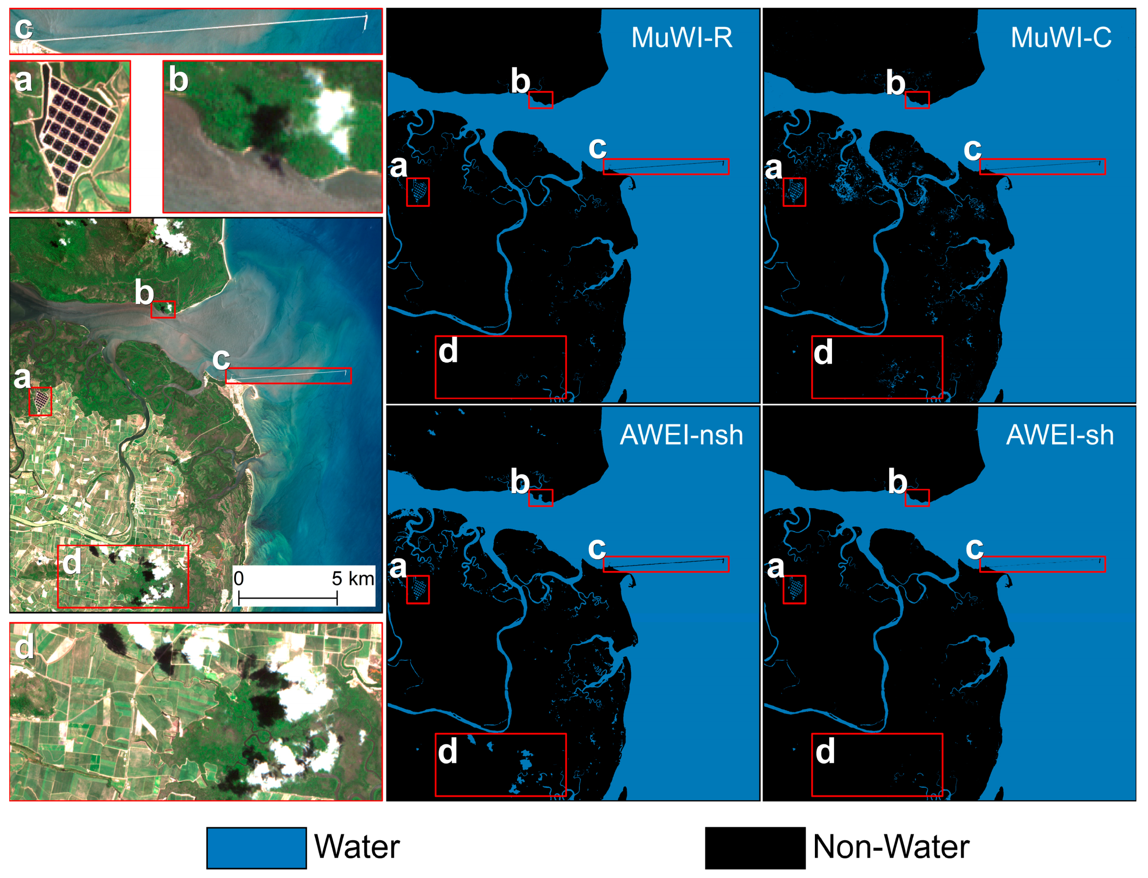
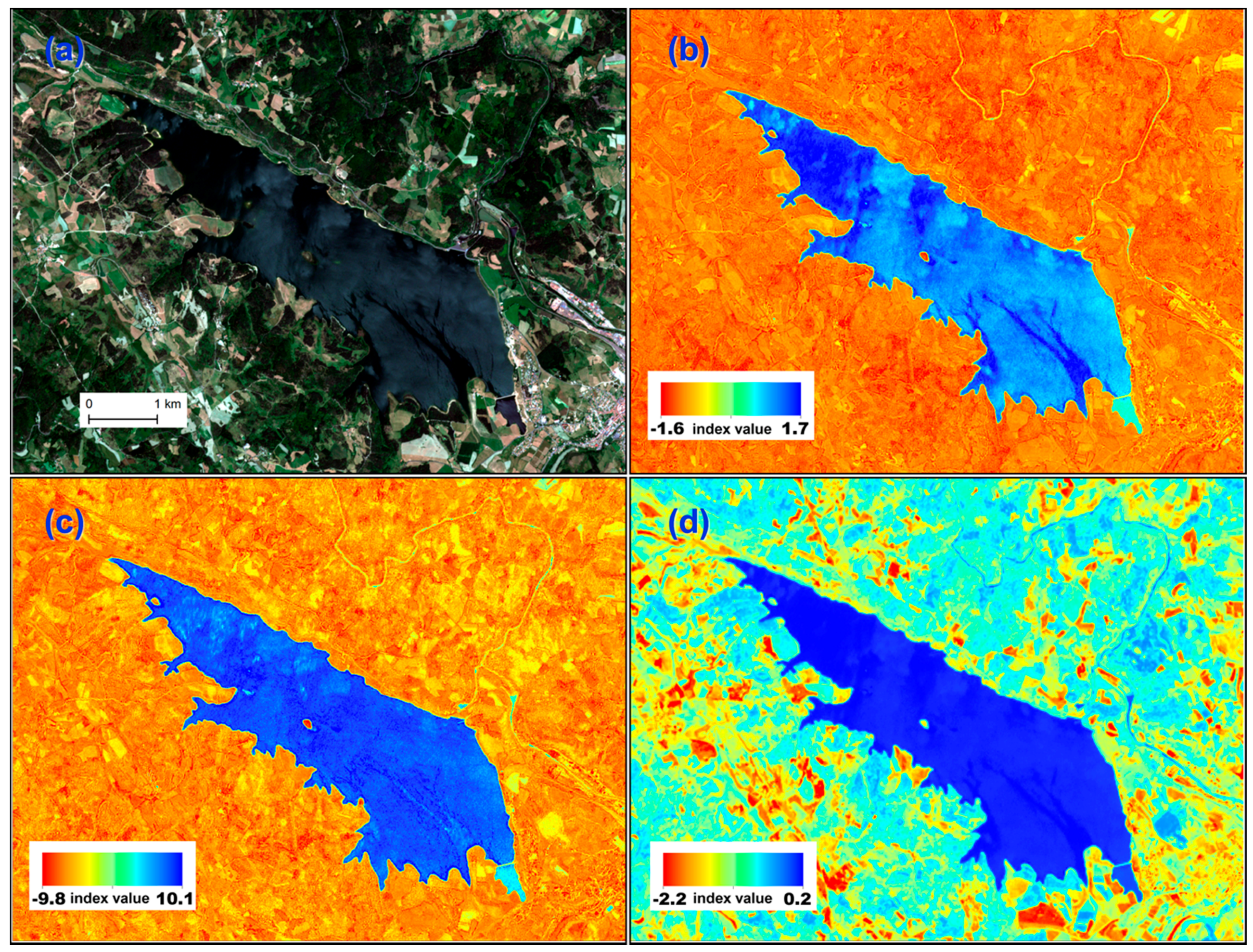
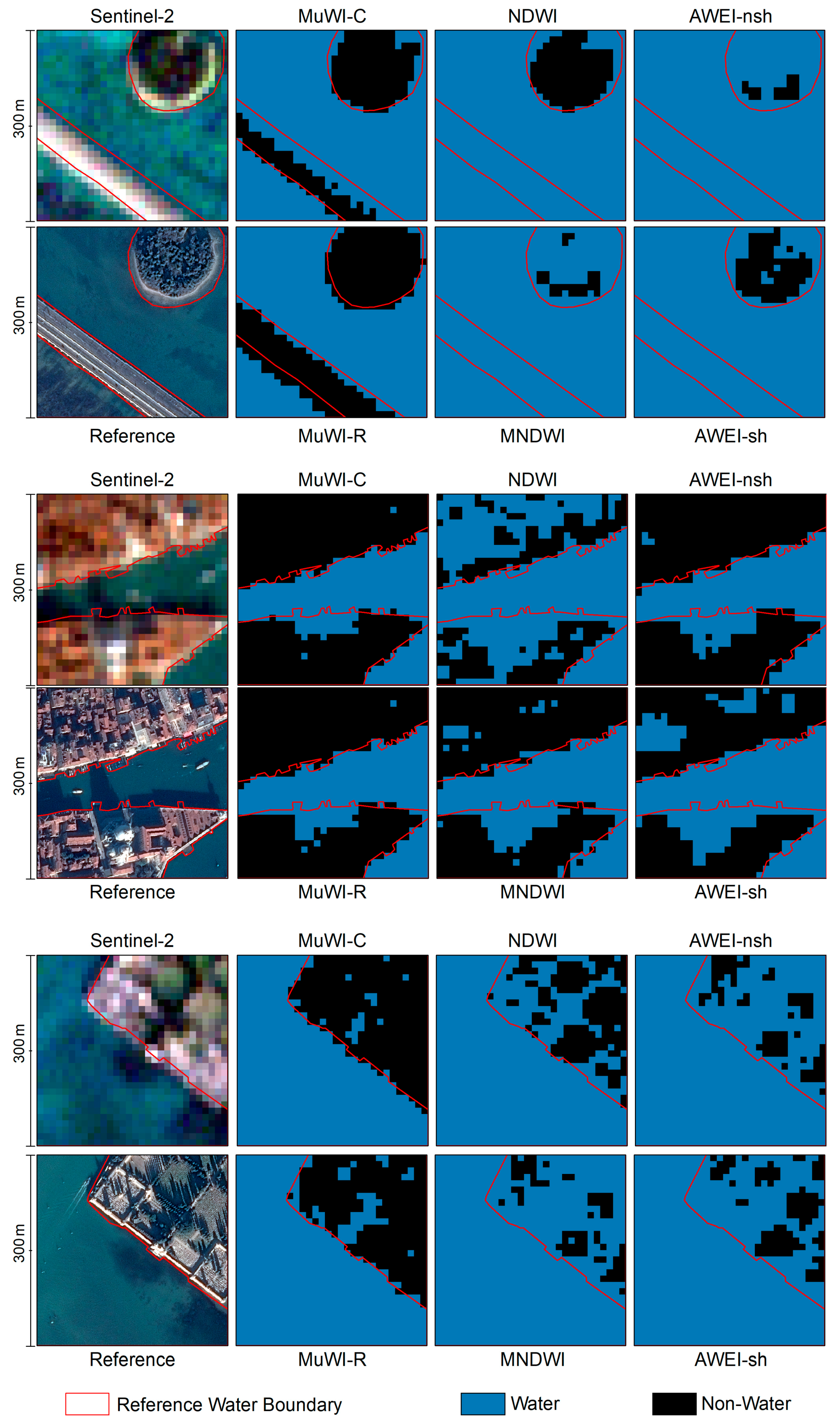
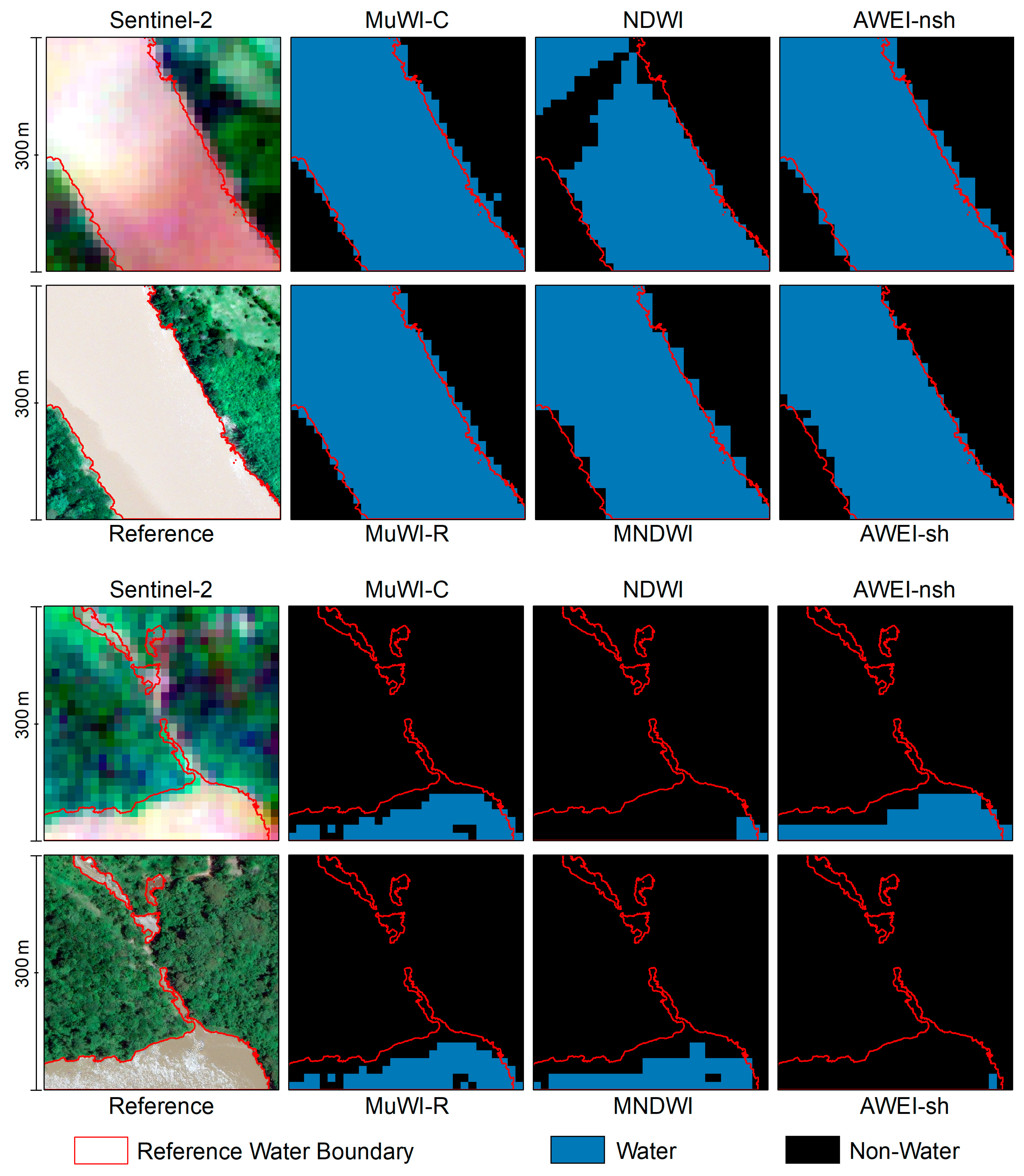
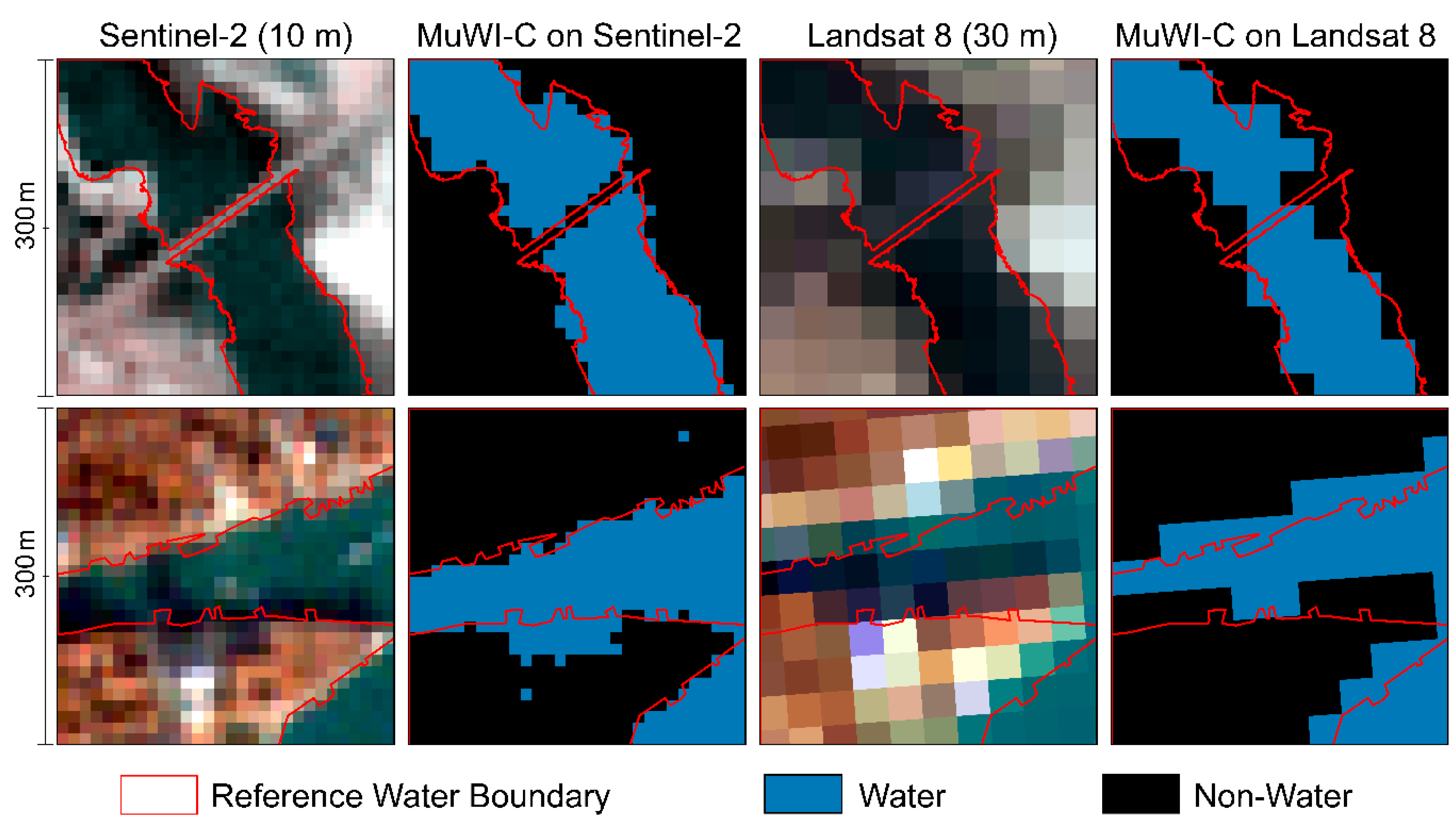
3.1. Qualitative Analysis

Figure 1 illustrates the water maps that are classified by two multi-spectral water index methods, MuWI and AWEI, on an estuary Sentinel-2 image (in eastern Australian: 146.39 E, −18.52 N, 19 February 2016). The image refers to an example in Harmel et al. (2018), where sunglint phenomenon is significant. Besides, various water bodies, as well as several patches of cloud shadow, are observed on the image. Thresholds are visually optimized to (1) accurately map the water pool grid (left red box), (2) make the dam (right red box) visible, and (3) minimize shadow misclassification (top and bottom red boxes). All water indexes can distinguish major river channel and ocean water. Both versions of MuWI correctly recognize shadow as non-water, whereas AWEI_nsh fails to classify most cloud shadows (the top and bottom red-box areas). The shadow-specified version of AWEI (AWEI_sh) can eliminate shadow errors, but it also omits some dark or vegetation-affected water bodies, as shown at peripheries of the tributary. The wetland areas, though, are well-detected by MuWI-R and MuWI-C, indicating that each single of MuWI can handle shadow issues and complex water bodies classification at the same time.

Figure 2 shows the values of three water indexes computed from a Sentinel-2 image over Naussac reservoir in France (3.81 E, 44.74 N, 7 July 2016, another example in Harmel et al. (2018)). The MuWI-R and MuWI-C maps show finer delineations for the boundary of the reservoir and other land covers, suggesting the potential of more accurate mapping. The ranges of MuWI-R and MuWI-C are [−1.6, 1.7] and [−9.8, 10.1], respectively, which is more asymmetric to zero in comparison to that of AWEI [−2.2, 0.2]. This implies that stable thresholding probably achieved using MuWI across different environmental settings. Although the sunglint contamination seems more apparent in MuWI-R map (b), it does not affect the classification, since the MuWI-R values of such areas are greater than the threshold.

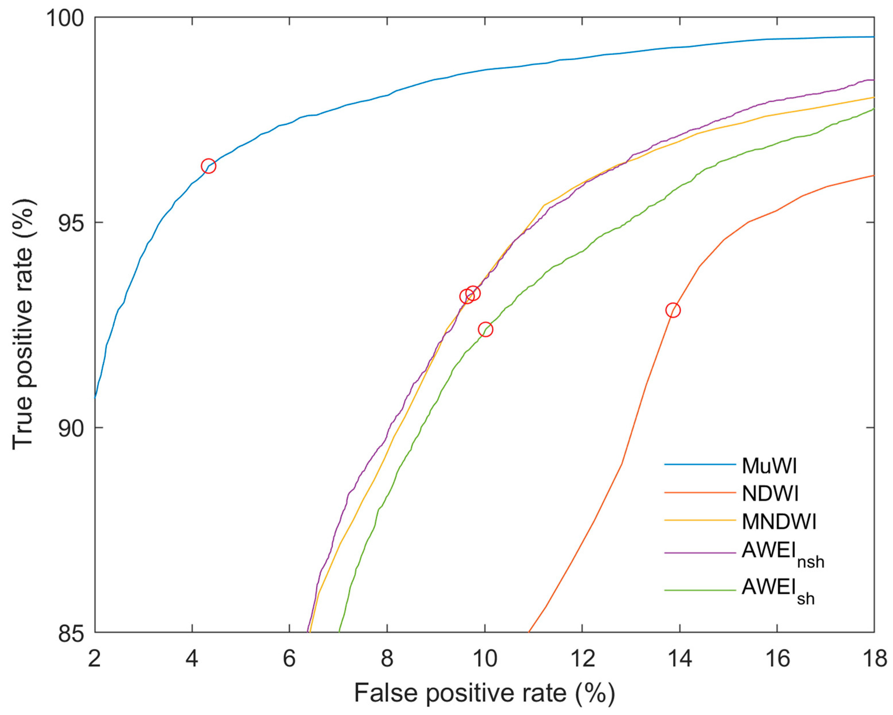
3.2. Quantitative Assessment

3.2.1. Statistical Accuracy Assessment

Table 3. Confusion matrixes of MuWI mapping results on (a) entire testing sites, (b) Venice testing sites, and (c) India testing sites.

(a) All Sites		Reference Classification
		Water	Non-Water	Accuracy
MuWI Classification	Water	18,715	1275	93.62%
	Non-Water	706	28,125	97.55%
	Accuracy	96.36%	95.66%	95.94%
(b) Venice Sites		Reference Classification
		Water	Non-Water	Accuracy
MuWI Classification	Water	9339	1000	90.33%
	Non-Water	116	5857	98.06%
	Accuracy	98.77%	85.42%	93.16%
(c) India Sites		Reference Classification
		Water	Non-Water	Accuracy
MuWI Classification	Water	6705	211	96.95%
	Non-Water	291	20,218	98.58%
	Accuracy	95.84%	98.97%	98.17%

lists confusion matrixes of MuWI-R on (a) entire testing sites, (b) Venice testing sites, and (c) India testing sites. Venice sites and India sites account for 90% of the all sites in total, with specific purposes of general inland-water testing and shadow confusion testing. A total of 48,821 pixels are tested, of which 40% are water pixels and 60% are non-water pixels. The OA of the classification for all sites, Venice sites, India sites are 96%, 93%, and 98%, respectively.

For all testing sites, commission error (non-water classified as water) is more prominent than omission error (water classified as non-water), reflected by the higher PA (96.36%, 1-omission error) and lower UA (93.62%, 1-commission error). Venice testing sites account for most of the commission error (1000 out of 1275 misclassified pixels) as most low-albedo settings, such as shadow and asphalt exist in this part of the dataset (like Figure S1). This high commission error leads to the relatively lowest accuracy for Venice sub-dataset. The India sub-dataset is close to the moderate water classification setting, where different water bodies (e.g., river, lake, pool, irrigation channel, reservoir) lie on varied underlying (e.g., forest, cropland, urban, bare-land). In the India sub-dataset, MuWI achieves high OA (98.17%), with balanced PA (95.84%) and UA (96.95%).

It is noted that the optimum thresholds for MuWI-R and other comparing water indexes are determined by the Receiver Operator Characteristics (ROC) curves (Figure 3). The red circles in Figure 3 denote where the optimum thresholds are found. The optimum position of MuWI-R among those of five water indexes is the closest to the top-left point, indicating the best tradeoff between the high true positive rate (TPR) and low false positive rate (FPR). However, the accuracy improvement of MuWI-R is rather evident: the TPR for MuWI-R is always greatest at the same FPR level, while the FPR lowest at the same TPR level. Because a constant term can be derived from OSH of SVM, the threshold for MuWI-C is directly determined as the negative constant term from OSH rather than determined by ROC curve. The optimum thresholds are used for water classification on all testing sites.

Table 4. Summary of the accuracy of MuWI and four water index methods.

	MuWI-C	MuWI-R	NDWI	MNDWI	AWEI-nsh	AWEI-sh
Overall Accuracy	96.42%	95.94%	88.81%	91.44%	91.30%	90.94%
Commission Error	4.85%	6.38%	18.44%	13.68%	12.44%	14.10%
Omission Error	4.11%	3.64%	7.15%	6.73%	8.93%	7.62%
Kappa Coefficient	92.54%	91.57%	77.17%	82.38%	81.97%	81.32%

compares accuracy of MuWI with that of NDWI, MNDWI, AWEI_nsh, and AWEI_sh by four measurements. MuWI-C, the completed version of MuWI, shows the highest OA (96.42%), followed by revised version MuWI-R (95.94%). Both versions of MuWI produce statistically better classification performance than the other four water indexes (p < 0.001). Commission errors of both MuWI are significantly reduced from greater than 10% to around 5% (4.85% and 6.38%). Lower omission errors of MuWI-C and MuWI-R are also observed. According to kappa coefficient, MuWI-C and MuWI-R present the highest consistency with the reference dataset. Overall, MuWI-C achieves the best performance of water classification, slightly exceeding MuWI-R, whilst both MuWI significantly improve the results when comparing to NDWI, MNDWI, AWEI-nsh and AWEI-sh.

However, given that the difference in accuracy and kappa coefficient of MuWI-C and MuWI-R are merely 0.48% and 0.96%, respectively, the McNemar test shows a high significance (p < 0.001) that MuWI-C performs better than MuWI-R. But, MuWI-R ignores less reference water pixels than MuWI-C as MuWI-R has a 0.48% lower omission error.

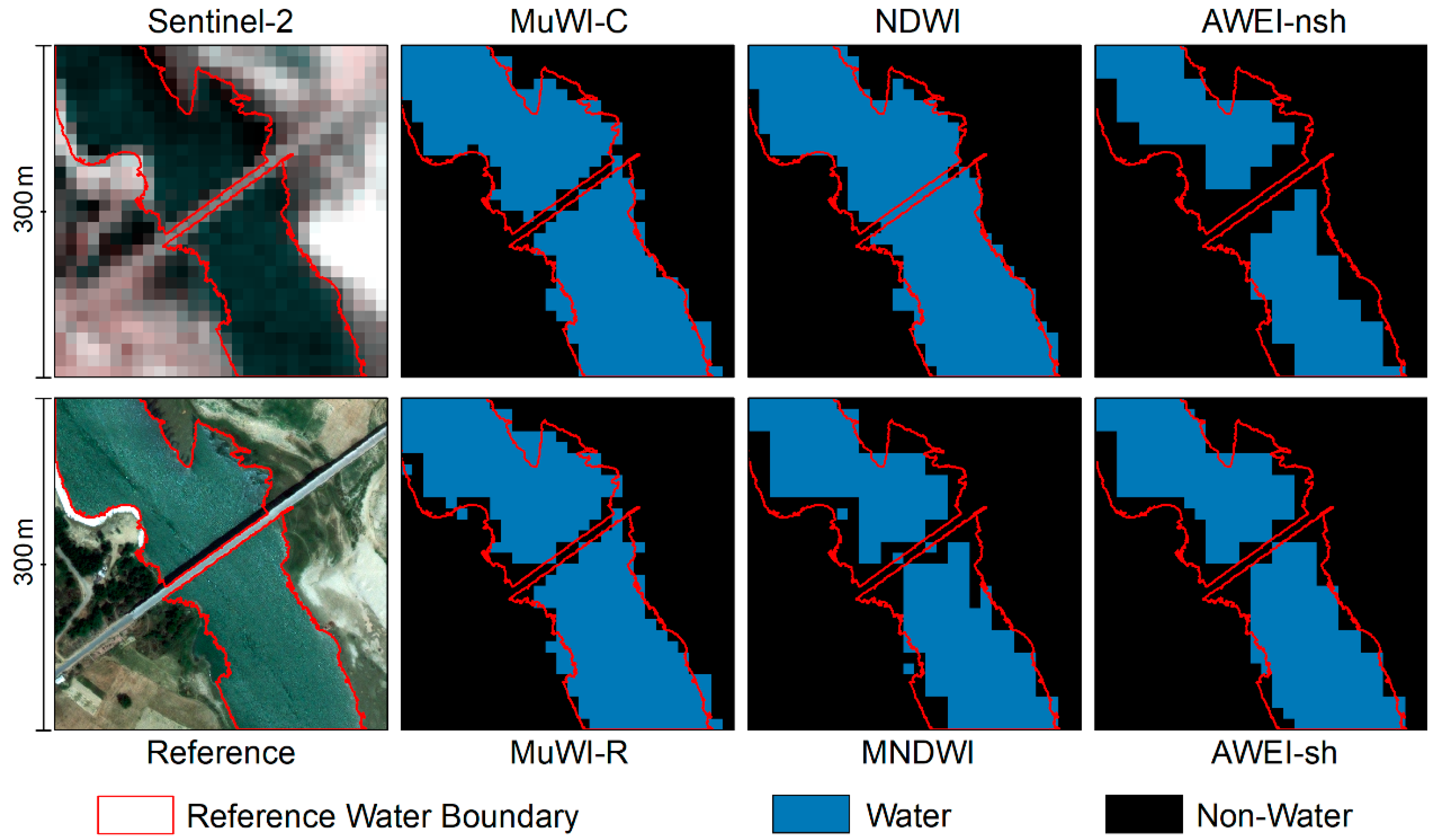
3.2.2. Comparison at Reference Site Level

In order to identify the specific differences of water classification results from different water indexes, the water maps of six 300 m-by-300 m reference sites are illustrated in terms of pixel size (Figure 4), low-albedo confusion (Figure 5), and sunglint contamination (Figure 6), respectively. For Figure 4, Figure 5 and Figure 6, 10-m Sentinel-2 RGB images and 0.5-m reference RGB images are also provided for visual inspections.

Figure 4 shows a testing site in northern India (top-left UTM coordinate: 722102, 2976724) where a highway bridge stands on the river with various vegetation, bare-land underlying. MuWI-C, MuWI-R and NDWI produce 10-m resolution outlines whilst MNDWI, AWEI-nsh and AWEI-sh produce 20-m resolution outlines. The resolution difference is related to different Sentinel-2 bands used by each water index. For example, NDWI adopts band 3 (10-m) and band 8 (10-m), but MNDWI corresponds to band 3 (10-m) and band 11 (20-m) so that MNDWI map present coarser outline of water bodies. Both MuWIs do utilize 20-m band (band 11 and band 12), yet the generated maps are in 10-m resolution, probably implying information of the selected 10-m band of MuWIs is sufficiently exploited and highly weighted for water classification. It may also be notable that the bridge can be detected by MuWI-C and MuWI-R but not by NDWI among three 10-m presentations. In this context, accuracies for 10-m indexes (MuWI-C: 94.2%, MuWI-R: 92.6%, NDWI: 95.3%) is higher than those for 20-m indexes (MNDWI: 88.7%, AWEI_nsh: 84.7%, AWEI_sh: 90.0%).

Figure 5 illustrates a wide asphalt road that connects mainland and lagoon area of Venice, which is one typical low-albedo underlying that is often misclassified as water. The water classification results are obvious that only MuWI-C and MuWI-R classify the asphalt road as non-water. Furthermore, a highly vegetated island surrounded by green ocean water is properly mapped by MuWI-C, MuWI-R and NDWI, yet poorly mapped by the rest of three water indexes. Regarding another low-albedo confusion, shadows are observed in the dense urban area (Figure 5 middle) and the sparsely vegetated garden (Figure 5 bottom). MuWI-C performs best for both shadow sites, having distinguished most of the shadow-affected area. MuWI-R presents more errors around the deep-dark non-water pixels for both sites, but the errors are relatively acceptable. AWEI_nsh presents similar maps of the middle urban-shadow site in Figure 5. However, the commission errors of other maps in both sites are significantly greater where large areas of shadow are misclassified as water.

Figure 6 contains sites where water bodies are observed with a partial area of abnormally high reflectance, which very likely results from the sunglint phenomenon. The Sentinel-2 image of top sites in Figure 6 shows a nearly-white triangular area on the flooded river. NDWI map fails to classify such a bright area correctly. The silvery water area on bottom site in Figure 6 is falsely little illustrated by NDWI and AWEI_sh classifications. MuWI-C and MuWI-R are able to detect water pixels in two sites under sunglint contamination.

4. Discussion

Spatial resolution is critical to accurate water mapping, thus likely to be an important source of accuracy improvements for MuWI. The native discrepancy of spatial resolution of Sentinel-2 bands often leads to the 20-m resolution in water mapping when using current water indexes, whereas the finest 10-m resolution of Sentinel-2 is not well-exploited. Previous studies [27,28] adopted band sharpening techniques to produce 10-m water map. But, band sharpening requires additional processing that is computationally intensive, thus time-consuming particularly for water mapping at large scale. NDWI coincidently uses two native 10-m bands on Sentinel-2, but its disadvantages have been long reported [22,23], particularly regarding commission errors. In the MuWI development, all four 10-m bands of Sentinel-2 were selected as input features. Meanwhile, the weights of 10-m bands were substantially enhanced in SVM training even though 20-m bands were also introduced. Consequently, the band selection and machine learning process ensure MuWI to adequately exploit information in the 10-m band for water mapping, so that MuWI produces inherent 10-m water maps without additional band sharpening.

Higher spatial resolution brings issues to water mapping, among which sunglint is one of the most notable. Sunglint is a special water-sensing issue that is becoming more apparent with the increased spatial resolution [48]. Few studies have focused on such a phenomenon on the widely-used Landsat series imagery with 30-m resolution. Atmospheric correction algorithms that aim to generate surface reflectance (SR) or bottom-of-atmosphere (BOA) products that were adopted by NASA or ESA do not include sunglint removal for Landsat [49] or Sentinel-2 imagery [32], respectively. This rather common phenomenon explained by Fresnel’s equation has been extensively studied in the ocean field [30], but has not been raised in water mapping prior to this study. On the other hand, water mapping essentially assumes water as a low-albedo feature yet sunglint increases reflectance from water area, which potentially contributes to omission error. Harmel et al. (2018) firstly introduces a sunglint correction method for Sentinel-2 imagery, but it cannot directly apply to index-based water mapping method because ancillary data (atmospheric parameters, climate data) are required. However, the idea of using SWIR bands (band 11, band 12 of Sentinel-2) from Harmel et al. (2018) for sunglint correction agrees with the band selection of MuWI that consists of the SWIR bands. It is observed that sunglint tends to occur at confluences, oxbows (Figure 6), in addition to the estuary (Figure 1) and windy water surface (Figure 2). MuWI manages to reduce the impacts from sunglint by deliberately introducing SWIR bands to the index formation and achieves the satisfactory mapping results over sunglint contamination areas. Depending on whether or not the SWIR bands are included, MNDWI and AWEI maps are less contaminated, but NDWI has more obvious sunglint issue. That is why the 20 m SWIR bands need to be retained in water indexes. In the situations that image-level sunglint reflectance correction as Harmel et al. (2018) is not easily implemented by users, the inclusion of SWIR bands for water mapping is necessary and effective.

Other than the new sunglint issue, shadow confusion—the misclassification of shadow as water—has long been identified as the most significant source of commission error in water mapping [8,22,23]. Shadows are mostly cast from built-up, vegetation at a fine scale, and terrain and cloud at both fine and coarse scale. In water mapping by 10-m Sentinel-2 imagery, the fine-scale shadows would be more confused and coarse-scale shadows still exist. Results of this study demonstrate the accuracy improvement of MuWI on shadow commission error (Table 2 and Figure 5). Shadow reflects low radiance across all visible and infrared wavelengths, but the reflective patterns over different spectral bands differ [23]. As a result, more bands combined by adequate formations could theoretically improve the detection of shadow, and further reduce shadow commission errors in water mapping. Previous multi-band indexes have also shown lower commission error when compared to dual-band indexes in different testing scenarios. The low commission error of MuWI, consequently, could attributed to multi-bands used and associated coefficients specified by machine learning.

Extremes conditions, like high-albedo water (e.g., sunglint) and low-albedo non-water (e.g., shadow), originate errors, while the thresholding process directly affects the classification accuracy [35]. Thresholding is related to water index forms. For example, the indexes with a form of normalized difference (e.g., NDWI and MNDWI) are constrained within [−1, 1], where their thresholds are close to zero. In contrast, thresholds of arithmetic forms (e.g., AWEI) have larger ranges. Many optimization algorithms have been conjunct with water index to determine thresholds [50]. However, the inherent issue of water index regarding thresholding should be the lack of threshold stability [23], meaning that the threshold for a particular type of water body under a particular environmental condition is not suitable for other types of water bodies under different environmental conditions. Threshold stability is especially important when conducting water mapping across large areas because complex land cover settings are more likely to exist. In this study, higher accuracy could be achieved if adjusting thresholds locally (e.g., all indexes across one of testing sites in Figure 4, Figure 5 and Figure 6), but the locally optimized thresholds lead to global accuracy reduction, since the used thresholds are optimized globally (by ROC curve in Figure 3). MuWI shows highest threshold stability perhaps because (1) the multi-band design makes MuWI more endogenously compatible with various types of water bodies under complex environments, (2) the basic normalized difference form reduces outlier interruptions. The former is also reflected by the evolvement of water index methods using increasing number of spectral bands [8]. The latter is supported by not only water index like NDWI and MNDWI, but also normalized difference index for other uses, like NDVI (Normalized Difference Vegetation Index).

In regard to methodology, this study, in a broader context, demonstrates a pathway to transfer machine-learned outcomes into simple index method that has been massively adopted in remote sensing. Machine learning algorithms train the model by supervised learning. The trained model is usually either a black-box, or too high-dimensional to know the mechanism inside [51]. The trained model may perform well but what the model has learned is little known to human users, which limits further usages. On the other hand, the index-based methods can be regarded as dimension reductions, which reduces multiple dimensions (of spectral bands) into one dimension (of the index). In development, the internal optimal separating hyperplane (OSH) in SVM was found among many machine learning algorithms, and was used for deriving water index where an explicit equation is obtained from sophiscated training process. Such a pathway between SVM and MuWI demonstrated in this study explores how to utilize effective machine learning algorithms for developing a simple index-based method in remote sensing classification. Potential uses are not only in water mapping but other binary classifications, such as urban area identification.

MuWI is discussed collectively aforementioned, but two versions of MuWI, MuWI-C and MuWI-R differ in expression, performance, and application. In general, the more complex MuWI-C performs better than simpler MuWI-R according to our test results. Notwithstanding, MuWI-R and MuWI-C achieve the two highest accuracies in the testing. Due to brevity and more significant reduction in certain omission errors, MuWI-R is recommended for the general water mapping usages, while MuWI-C is recommended if the water mapping application pursues the highest possible OA.

MuWI is developed on Sentinel-2 imagery, and could be arguably applied on Landsat imagery. All six Sentinel-2 bands involved in MuWI (band 2, 3, 4, 8, 11, 12) could map to bands on Landsat 5, 7 and 8 (

Table 5. The mapping relationships between Sentinel-2 bands and Landsat bands.

Sentinel-2 Band	Landsat 8 OLI Band	Landsat 7/5 ETM+/TM Band
1	1	none
2	2	1
3	3	2
4	4	3
5	none	none
6	none	none
7	none	4
8	5	4
8A	5	4
9	none	none
10	9	none
11	6	5
12	7	7

). Based on the bands mapping, Figure 7 demonstrate the easily transferable use of MuWI on Landsat sensors. Similar water patterns can be found across two reference sites in Venice when applying MuWI on Landsat 8 OLI image, but coarser results are obvious due to Landsat 8 30 m resolution. However, similar to [24], more systematic examinations of using MuWI on other sensors (such as Landsat, SPOT-5, Gaofen-2, MODIS) with quantitative analysis over large samples remain necessary. Applying MuWI on multi-sensor image fusion would increase the temporal resolution of water mapping, but that work (MuWI on fusion) may be beyond the scope of this paper (MuWI development), and will hopefully present in another paper.

Uncertainties that are involved in this study are mainly attributable to the processing of Sentinel-2 spectral reflectance, and the temporal differences of water extents in validation images. Surface reflectance (or BOA reflectance) rather than TOA reflectance theoretically delineates surface water more accurately. The atmospheric impacts, such as cirrus, may significantly degrade the water mapping results when using TOA reflectance. However, those impacts could be hedged by cloud-cover filtering, and heavily-used normalized difference forms in this study. One comparative study on the impact of Landsat TOA and surface reflectance found no outstanding differences in water mapping results in many cases [24]. But, surface reflectance would reduce the uncertainty from atmospheric disturbances. Although the validation images were selected to best ensure capture time closeness to that of Sentinel-2 images (0 to 5 days in the study), temporal variations of water bodies could introduce uncertainty to the validation, particularly of coastal areas.

Though the testing sites are selected with considerations to represent different water bodies under different settings, more sites from different regions of the world need to be tested. It is particular for the water bodies with high vegetation impacts, such as wetlands and areas that are concentrated with high chlorophyll or covered with alga. The difficulties to eliminate vegetated confusions in water mapping have long been identified [52,53,54], and have also been observed in this study (e.g., wetlands in Venice). Impacts of vegetations are not specially tested in this study, yet they may considerably affect water mapping, which deserve further studies in future. The bands of 10-m resolution and SWIR bands are adopted in MuWI, but an exhaustive study on water reflective patterns of every Sentinel-2 bands will probably provide more details for revising the water index. Furthermore, the feature selection process in machine learning in this study is subjective to prior knowledge, a combined automated feature selection [55] may shed lights on further enhancement of developing remote sensing index method in the future.

5. Conclusions

This study proposed a new automated water index method MuWI with the ability to natively produce 10 m water maps on Sentinel-2 MSI imagery. The methodological strength of the study is mainly the use of a machine learning algorithm SVM for objective, explicit index development. Accuracy comparisons among Landsat-developed water index methods showed that the proposed MuWI method produced water maps with increased spatial resolution (10-m) and lowered commission and omission errors. This could be owed to the adequate exploitation of native 10-m Sentinel-2 spectral bands as well as significant reductions in shadow and sunglint misclassifications. But, aquatic enclaves that mix with masses of algae or macrophytes still show significant confusions for all indexes. Complete version index MuWI-C was proposed for achieving the highest overall accuracy, while revised version MuWI-R was proposed as an improved trade-off between accuracy and simplicity. The proposed method will possibly facilitate accurate water mapping on growing Sentinel-2 images and further broad applications.

References

1. Sadeghi, M.; Babaeian, E.; Tuller, M.; Jones, S.B. The optical trapezoid model: A novel approach to remote sensing of soil moisture applied to Sentinel-2 and Landsat-8 observations. Remote Sens. Environ. 2017, 198, 52–68. [Google Scholar] [CrossRef] [Green Version]
2. Veloso, A.; Mermoz, S.; Bouvet, A.; Le Toan, T.; Planells, M.; Dejoux, J.F.; Ceschia, E. Understanding the temporal behavior of crops using Sentinel-1 and Sentinel-2-like data for agricultural applications. Remote Sens. Environ. 2017, 199, 415–426. [Google Scholar] [CrossRef]
3. Pahlevan, N.; Sarkar, S.; Franz, B.A.; Balasubramanian, S.V.; He, J. Sentinel-2 MultiSpectral Instrument (MSI) data processing for aquatic science applications: Demonstrations and validations. Remote Sens. Environ. 2017, 201, 47–56. [Google Scholar] [CrossRef]
4. Puliti, S.; Saarela, S.; Gobakken, T.; Ståhl, G.; Næsset, E. Combining UAV and Sentinel-2 auxiliary data for forest growing stock volume estimation through hierarchical model-based inference. Remote Sens. Environ. 2018, 204, 485–497. [Google Scholar] [CrossRef]
5. Jakimow, B.; Griffiths, P.; van der Linden, S.; Hostert, P. Mapping pasture management in the Brazilian Amazon from dense Landsat time series. Remote Sens. Environ. 2018, 205, 453–468. [Google Scholar] [CrossRef]
6. Gómez, C.; White, J.C.; Wulder, M.A. Optical remotely sensed time series data for land cover classification: A review. ISPRS J. Photogramm. Remote Sens. 2016, 116, 55–72. [Google Scholar] [CrossRef]
7. Brezonik, P.L.; Olmanson, L.G.; Finlay, J.C.; Bauer, M.E. Factors affecting the measurement of CDOM by remote sensing of optically complex inland waters. Remote Sens. Environ. 2015, 157, 199–215. [Google Scholar] [CrossRef]
8. Pekel, J.-F.; Cottam, A.; Gorelick, N.; Belward, A.S. High-resolution mapping of global surface water and its long-term changes. Nature 2016, 540, 418–422. [Google Scholar] [CrossRef] [PubMed]
9. Donchyts, G.; Baart, F.; Winsemius, H.; Gorelick, N.; Kwadijk, J.; Van De Giesen, N. Earth’s surface water change over the past 30 years. Nat. Clim. Chang. 2016, 6, 810–813. [Google Scholar] [CrossRef]
10. Müller, M.F.; Yoon, J.; Gorelick, S.M.; Avisse, N.; Tilmant, A. Impact of the Syrian refugee crisis on land use and transboundary freshwater resources. Proc. Natl. Acad. Sci. USA 2016, 113, 14932–14937. [Google Scholar] [CrossRef] [PubMed]
11. Arino, O.; Ramos Perez, J.J.; Kalogirou, V.; Bontemps, S.; Defourny, P.; Van Bogaert, E. Global Land Cover Map for 2009 (GlobCover 2009); European Space Agency (ESA): Paris, France; Université Catholique de Louvain (UCL) PANGAEA: Louvain-la-Neuve, Belgium, 2012. [Google Scholar] [CrossRef]
12. Chen, J.; Chen, J.; Liao, A.; Cao, X.; Chen, L.; Chen, X.; He, C.; Han, G.; Peng, S.; Lu, M.; et al. Global land cover mapping at 30 m resolution: A POK-based operational approach. ISPRS J. Photogramm. Remote Sens. 2014, 103, 7–27. [Google Scholar] [CrossRef]
13. Smith, M.W.; Macklin, M.G.; Thomas, C.J. Hydrological and geomorphological controls of malaria transmission. Earth Sci. Rev. 2013, 116, 109–127. [Google Scholar] [CrossRef]
14. Dottori, F.; Salamon, P.; Bianchi, A.; Alfieri, L.; Hirpa, F.A.; Feyen, L. Development and evaluation of a framework for global flood hazard mapping. Adv. Water Resour. 2016, 94, 87–102. [Google Scholar] [CrossRef] [Green Version]
15. Liu, J.; Shi, Z.; Wang, D. Measuring and mapping the flood vulnerability based on land-use patterns: A case study of Beijing, China. Nat. Hazards 2016, 83, 1545–1565. [Google Scholar] [CrossRef]
16. Vanham, D.; Hoekstra, A.Y.; Wada, Y.; Bouraoui, F.; de Roo, A.; Mekonnen, M.M.; van de Bund, W.J.; Batelaan, O.; Pavelic, P.; Bastiaanssen, W.G.M.; et al. Physical water scarcity metrics for monitoring progress towards SDG target 6.4: An evaluation of indicator 6.4.2 “Level of water stress”. Sci. Total Environ. 2018, 613–614, 218–232. [Google Scholar] [CrossRef] [PubMed]
17. Olmanson, L.G.; Brezonik, P.L.; Finlay, J.C.; Bauer, M.E. Comparison of Landsat 8 and Landsat 7 for regional measurements of CDOM and water clarity in lakes. Remote Sens. Environ. 2016, 185, 119–128. [Google Scholar] [CrossRef]
18. Feng, M.; Sexton, J.O.; Channan, S.; Townshend, J.R. A global, high-resolution (30-m) inland water body dataset for 2000: First results of a topographic–spectral classification algorithm. Int. J. Digit. Earth 2016, 9, 113–133. [Google Scholar] [CrossRef]
19. Verpoorter, C.; Kutser, T.; Seekell, D.A.; Tranvik, L.J. A global inventory of lakes based on high-resolution satellite imagery. Geophys. Res. Lett. 2014, 41, 6396–6402. [Google Scholar] [CrossRef] [Green Version]
20. Zou, Z.; Xiao, X.; Dong, J.; Qin, Y.; Doughty, R.B.; Menarguez, M.A.; Zhang, G.; Wang, J. Divergent trends of open-surface water body area in the contiguous United States from 1984 to 2016. Proc. Natl. Acad. Sci. USA 2018, 201719275. [Google Scholar] [CrossRef] [PubMed]
21. McFeeters, S.K. The use of the Normalized Difference Water Index (NDWI) in the delineation of open water features. Int. J. Remote Sens. 1996, 17, 1425–1432. [Google Scholar] [CrossRef]
22. Xu, H. Modification of normalised difference water index (NDWI) to enhance open water features in remotely sensed imagery. Int. J. Remote Sens. 2006. [Google Scholar] [CrossRef]
23. Feyisa, G.L.; Meilby, H.; Fensholt, R.; Proud, S.R. Automated Water Extraction Index: A new technique for surface water mapping using Landsat imagery. Remote Sens. Environ. 2014, 140, 23–35. [Google Scholar] [CrossRef]
24. Fisher, A.; Flood, N.; Danaher, T. Comparing Landsat water index methods for automated water classification in eastern Australia. Remote Sens. Environ. 2016, 175, 167–182. [Google Scholar] [CrossRef]
25. Crist, E.P. A TM Tasseled Cap equivalent transformation for reflectance factor data. Remote Sens. Environ. 1985. [Google Scholar] [CrossRef]
26. Domenikiotis, C. The use of NOAA/AVHRR satellite data for monitoring and assessment of forest fires and floods. Nat. Hazards Earth Syst. Sci. 2003. [Google Scholar] [CrossRef]
27. Yang, X.; Zhao, S.; Qin, X.; Zhao, N.; Liang, L. Mapping of urban surface water bodies from sentinel-2 MSI imagery at 10 m resolution via NDWI-based image sharpening. Remote Sens. 2017, 9, 596. [Google Scholar] [CrossRef]
28. Du, Y.; Zhang, Y.; Ling, F.; Wang, Q.; Li, W.; Li, X. Water bodies’ mapping from Sentinel-2 imagery with Modified Normalized Difference Water Index at 10-m spatial resolution produced by sharpening the swir band. Remote Sens. 2016, 8, 354. [Google Scholar] [CrossRef] [Green Version]
29. Cox, C.; Munk, W. Measurement of the Roughness of the Sea Surface from Photographs of the Sun’s Glitter. J. Opt. Soc. Am. 1954, 44, 838. [Google Scholar] [CrossRef]
30. Jackson, C. Internal wave detection using the Moderate Resolution Imaging Spectroradiometer (MODIS). J. Geophys. Res. 2007, 112, C11012. [Google Scholar] [CrossRef]
31. Overstreet, B.T.; Legleiter, C.J. Removing sun glint from optical remote sensing images of shallow rivers. Earth Surf. Process. Landf. 2017, 42, 318–333. [Google Scholar] [CrossRef]
32. Gascon, F.; Bouzinac, C.; Thépaut, O.; Jung, M.; Francesconi, B.; Louis, J.; Lonjou, V.; Lafrance, B.; Massera, S.; Gaudel-Vacaresse, A.; et al. Copernicus Sentinel-2A calibration and products validation status. Remote Sens. 2017, 9, 584. [Google Scholar] [CrossRef]
33. Harmel, T.; Chami, M.; Tormos, T.; Reynaud, N.; Danis, P.A. Sunglint correction of the Multi-Spectral Instrument (MSI)-SENTINEL-2 imagery over inland and sea waters from SWIR bands. Remote Sens. Environ. 2018, 204, 308–321. [Google Scholar] [CrossRef] [Green Version]
34. Huang, C.; Chen, Y.; Zhang, S.; Wu, J. Detecting, Extracting, and Monitoring Surface Water From Space Using Optical Sensors: A Review. Rev. Geophys. 2018. [Google Scholar] [CrossRef]
35. Ji, L.; Zhang, L.; Wylie, B. Analysis of Dynamic Thresholds for the Normalized Difference Water Index. Photogramm. Eng. Remote Sens. 2009, 75, 1307–1317. [Google Scholar] [CrossRef]
36. Huang, X.; Xie, C.; Fang, X.; Zhang, L. Combining Pixel-and Object-Based Machine Learning for Identification of Water-Body Types from Urban High-Resolution Remote-Sensing Imagery. IEEE J. Sel. Top. Appl. Earth Obs. Remote Sens. 2015, 8, 2097–2110. [Google Scholar] [CrossRef]
37. Isikdogan, F.; Bovik, A.C.; Passalacqua, P. Surface water mapping by deep learning. IEEE J. Sel. Top. Appl. Earth Obs. Remote Sens. 2017, 10, 4909–4918. [Google Scholar] [CrossRef]
38. Whyte, A.; Ferentinos, K.P.; Petropoulos, G.P. A new synergistic approach for monitoring wetlands using Sentinels-1 and 2 data with object-based machine learning algorithms. Environ. Model. Softw. 2018, 104, 40–54. [Google Scholar] [CrossRef]
39. Cortes, C.; Vapnik, V. Support Vector Networks. Mach. Learn. 1995, 20, 273–297. [Google Scholar] [CrossRef]
40. Felzenszwalb, P.F.; Girshick, R.B.; Mcallester, D.; Ramanan, D. Object Detection with Discriminatively Trained Part Based Models. IEEE Trans. Pattern Anal. Mach. Intell. 2009, 32, 1–20. [Google Scholar] [CrossRef] [PubMed]
41. Foody, G.M.; Mathur, A. The use of small training sets containing mixed pixels for accurate hard image classification: Training on mixed spectral responses for classification by a SVM. Remote Sens. Environ. 2006, 103, 179–189. [Google Scholar] [CrossRef]
42. Mountrakis, G.; Im, J.; Ogole, C. Support vector machines in remote sensing: A review. ISPRS J. Photogramm. Remote Sens. 2011, 66, 247–259. [Google Scholar] [CrossRef]
43. Nogueira, K.; Penatti, O.A.B.; dos Santos, J.A. Towards better exploiting convolutional neural networks for remote sensing scene classification. Pattern Recognit. 2017, 61, 539–556. [Google Scholar] [CrossRef] [Green Version]
44. Bennett, K.P.; Campbell, C. Support vector machines: Hype or Hallelujah? ACM SIGKDD Explor. Newsl. 2000. [Google Scholar] [CrossRef]
45. Chang, C.-C.; Lin, C.-J. A Library for Support Vector Machines. ACM Trans. Intell. Syst. Technol. 2011, 2, 39. [Google Scholar] [CrossRef]
46. Ko, B.C.; Kim, H.H.; Nam, J.Y. Classification of Potential Water Bodies Using Landsat 8 OLI and a Combination of Two Boosted Random Forest Classifiers. Sensors 2015, 15, 13763–13777. [Google Scholar] [CrossRef] [PubMed] [Green Version]
47. de Leeuw, J.; Jia, H.; Yang, L.; Liu, X.; Schmidt, K.; Skidmore, A.K. Comparing accuracy assessments to infer superiority of image classification methods. Int. J. Remote Sens. 2006. [Google Scholar] [CrossRef]
48. Kay, S.; Hedley, J.D.; Lavender, S. Sun glint correction of high and low spatial resolution images of aquatic scenes: A review of methods for visible and near-infrared wavelengths. Remote Sens. 2009, 1, 697–730. [Google Scholar] [CrossRef]
49. Roy, D.P.; Kovalskyy, V.; Zhang, H.K.; Vermote, E.F.; Yan, L.; Kumar, S.S.; Egorov, A. Characterization of Landsat-7 to Landsat-8 reflective wavelength and normalized difference vegetation index continuity. Remote Sens. Environ. 2016, 185, 57–70. [Google Scholar] [CrossRef]
50. Gamshadzaei, M.H.; Rahimzadegan, M. Stable and accurate methods for identification of water bodies from Landsat series imagery using meta-heuristic algorithms. J. Appl. Remote Sens. 2017, 11, 045005. [Google Scholar] [CrossRef]
51. Rodriguez-Galiano, V.F.; Ghimire, B.; Rogan, J.; Chica-Olmo, M.; Rigol-Sanchez, J.P. An assessment of the effectiveness of a random forest classifier for land-cover classification. ISPRS J. Photogramm. Remote Sens. 2012, 67, 93–104. [Google Scholar] [CrossRef]
52. Mertes, L.A.K.; Daniel, D.L.; Melack, J.M.; Nelson, B.; Martinelli, L.A.; Forsberg, B.R. Spatial patterns of hydrology, geomorphology, and vegetation on the floodplain of the Amazon river in Brazil from a remote sensing perspective. Geomorphology 1995. [Google Scholar] [CrossRef]
53. Mayaux, P.; De Grandi, G.F.; Rauste, Y.; Simard, M.; Saatchi, S. Large-scale vegetation maps derived from the combined L-band GRFM and C-band CAMP wide area radar mosaics of Central Africa. Int. J. Remote Sens. 2002. [Google Scholar] [CrossRef]
54. Alsdorf, D.E.; Rodríguez, E.; Lettenmaier, D.P. Measuring surface water from space. Rev. Geophys. 2007, 45, RG2002. [Google Scholar] [CrossRef]
55. Nguyen, M.H.; de la Torre, F. Optimal feature selection for support vector machines. Pattern Recognit. 2010, 43, 584–591. [Google Scholar] [CrossRef] [Green Version]
Figure 1. Sentinel-2 RGB image and corresponding water maps classified by spectral water index (MuWI) and Automated Water Extraction Index (AWEI) over an estuary in eastern Australia. Red boxes indicate typical areas that are difficult for water mapping: cloud shadows (red boxes b & d), small water bodies (red box a), small objects on the water surface (red box c).
Remotesensing 10 01643 g001
Figure 2. Sentinel-2 RGB image (a) over Naussac reservoir (altitude: 940 m) in France and maps of index values of MuWI-R (b), MuWI-C (c), and AWEInsh (d) with minimum and maximum index values.
Remotesensing 10 01643 g002
Figure 3. Receiver Operator Characteristic (ROC) curves of water indexes. Red circles indicate the optimum index thresholds.
Remotesensing 10 01643 g003
Figure 4. A reference site with a bridge of approximate 10-m width. The first column shows 10-m Sentinel-2 RGB image and 0.5-m reference RGB image. Column 2, 3, and 4 shows the water mapping results by six water index (MuWI-C, MuWI-R, NDWI, MNDWI, AWEI-nsh, AWEI-sh).
Remotesensing 10 01643 g004
Figure 5. Three reference sites that are profoundly impacted by low-albedo confusions from asphalt (top), built-up shadow (middle) and vegetation shadow (bottom). The first column shows 10-m Sentinel-2 RGB image and 0.5-m reference RGB image. Column 2, 3, and 4 shows the water mapping results by six water index (MuWI-C, MuWI-R, NDWI, MNDWI, AWEI-nsh, AWEI-sh).
Remotesensing 10 01643 g005
Figure 6. Two reference sites with suspected sunglint contaminations at a confluence (top) and an oxbow (bottom) of the inland river. The first column shows 10-m Sentinel-2 RGB image and 0.5-m reference RGB image. Column 2, 3, and 4 shows the water mapping results by six water index (MuWI-C, MuWI-R, NDWI, MNDWI, AWEI-nsh, AWEI-sh).
Remotesensing 10 01643 g006
Figure 7. Visual comparisons of MuWI applications on Sentinel-2 and Landsat 8. Two rows indicate two 300 m × 300 m reference sites that are the same as in Figure 4 and Figure 5. Four columns represent (from left to right): Sentinel-2 MSI RGB (4, 3, 2) 10 m natural color image, MuWI-C classified result on Sentinel-2, Landsat 8 OLI RGB(4, 3, 2) 30 m natural color image, and MuWI-C classified result on Landsat 8.
Remotesensing 10 01643 g007