Article

Using Time Series of High-Resolution Planet Satellite Images to Monitor Grapevine Stem Water Potential in Commercial Vineyards

1
Institute of Agricultural Engineering, Agricultural Research Organization (Volcani Center), P.O. Box 15159, Rishon LeZion 7505101, Israel
2
Department of Geography and the Environment, Bar-Ilan University, Ramat Gan 5290002, Israel
3
Institute of Plant Sciences and Genetics in Agriculture, The Robert H. Smith Faculty of Agriculture, Food & Environment, The Hebrew University of Jerusalem, Rehovot 76100, Israel
4
Department of Agriculture and Oenology, Eastern R&D Center, Ariel 40700, Israel
5
Department of Chemistry & Biotech Engineering, Ariel University, Ariel 40700, Israel
6
Department of Soil, Water and Environmental Sciences, Agricultural Research Organization Gilat Research Center, Mobile post Negev, Gilat 8531100, Israel
7
TerraVision Lab, Midreshet Ben-Gurion 8499000, Israel
*
Author to whom correspondence should be addressed.
Remote Sens. 2018, 10(10), 1615; https://doi.org/10.3390/rs10101615
Submission received: 1 August 2018 / Revised: 20 September 2018 / Accepted: 9 October 2018 / Published: 11 October 2018
(This article belongs to the Special Issue High Resolution Image Time Series for Novel Agricultural Applications)

Abstract

:
Spectral-based vegetation indices (VI) have been shown to be good proxies of grapevine stem water potential (Ψstem), assisting in irrigation decision-making for commercial vineyards. However, VI-Ψstem correlations are mostly reported at the leaf or canopy scales, using proximal canopy-based sensors or very-high-spatial resolution images derived from sensors mounted on small airplanes or drones. Here, for the first time, we take advantage of high-spatial resolution (3-m) near-daily images acquired from Planet’s nano-satellite constellation to derive VI-Ψstem correlations at the vineyard scale. Weekly Ψstem was measured along the growing season of 2017 in six vines each in 81 commercial vineyards and in 60 pairs of grapevines in a 2.4 ha experimental vineyard in Israel. The Clip application programming interface (API), provided by Planet, and the Google Earth Engine platform were used to derive spatially continuous time series of four VIs—GNDVI, NDVI, EVI and SAVI—in the 82 vineyards. Results show that per-week multivariable linear models using variables extracted from VI time series successfully tracked spatial variations in Ψstem across the experimental vineyard (Pearson’s-r = 0.45–0.84; N = 60). A simple linear regression model enabled monitoring seasonal changes in Ψstem along the growing season in the vineyard (r = 0.80–0.82). Planet VIs and seasonal Ψstem data from the 82 vineyards were used to derive a ‘global’ model for in-season monitoring of Ψstem at the vineyard-level (r = 0.78; RMSE = 18.5%; N = 970). The ‘global’ model, which requires only a few VI variables extracted from Planet images, may be used for real-time weekly assessment of Ψstem in Mediterranean vineyards, substantially improving the efficiency of conventional in-field monitoring efforts.

Graphical Abstract

1. Introduction

Deficit irrigation is a commonly used irrigation strategy in vineyards aiming to achieve high-quality berries for premium wine production [1]. However, to optimize grape quality and production deficit, irrigation should be properly controlled. Proper irrigation management is also compulsory to achieve uniform quality of berries across the vineyard area. An effective method to guide irrigation management of wine grapes is continuous spatial (across the vineyard) and temporal (along the season) monitoring of grapevine water status [2]. Water status is typically quantified by measuring vine stem water potential (Ψstem), which provides an indication of the impact of soil water content on grapevine water status [3]. To achieve an accurate picture of the water status variability across the entire vineyard area, continuous Ψstem measurements are required from as many vines as possible. This task requires substantial human resources, making it time consuming.
Emerging precision agriculture tools such as proximal and remote sensing offer possible replacement, or at least support, of conventional in-field monitoring techniques [4,5]. Proximal and remote sensing tools may be used to provide the required information for irrigation management control [6], as well as to allow spatial consideration of irrigation needs across the crop field [7]. Remote and proximal sensing have been used for monitoring vegetation dynamics [8] and processes including water status [9,10,11], plant nutrient content [12,13], plant diseases [14,15] and crop phenotyping [16]. The information received from sensors mounted on drones or small airplanes can be applied to develop site-specific irrigation and other management decisions [17]. Thermal sensors mounted on airplanes or drones may provide information on plant water status through the use of the crop water stress index [18,19,20]. Crop water stress index (CWSI), which is based on crop canopy temperature [21], has been recognized as a reliable index for monitoring in-field water status variability within a vineyard area [22,23,24,25]. CWSI has been shown to correlate with Ψstem, though typically displaying different correlations for different dates along the season [26,27].
Another approach is to use vegetation indices (VIs) derived from spectral bands as proxies for water status parameters and/or yield production. For example, Espinoza et al. [28], found that the normalized difference vegetation index (NDVI) and the green normalized difference vegetation index (GNDVI) derived from very-high-spatial resolution images (2.6 cm) were both correlated with pre-harvest leaf stomatal conductance (gs; r = 0.56 and 0.65, respectively) and yield production (r = 0.68 and 0.73, respectively) in a cabernet sauvignon vineyard near Benton City, Washington. Baluja et al. [22] found strong correlations of spectral-based vegetation indices such as, GNDVI, NDVI and the modified simple ratio (MSR) with gs (r = 0.84, 0.87 and 0.88, respectively) and Ψstem (r = 0.76, 0.82 and 0.81, respectively) using images acquired from an unmanned aerial vehicle in a commercial rain-fed tempranillo vineyard in Spain. Their results imply that VIs can serve as good water stress indicators in vineyards when using very-high-spatial resolution images (10 cm) that allow the extraction of pure canopy pixels. As expected, they also found high correlations of thermal data with gs and Ψstem; however, the correlation changed along the season [22], meaning that a per-date calibration should be derived in order to provide recommendations for irrigation scheduling throughout the season.
Zarco-Tejada et al. [29] proposed a normalized photochemical reflectance index (PRInorm) using a combination of the re-normalized difference vegetation index (RDVI), which is sensitive to canopy structure, and a red edge index, sensitive to chlorophyll content (R700/R670), to detect xanthophyll pigment changes and normalize for leaf area and chlorophyll content level reduction induced by water stress. They found that PRInorm was highly correlated with midday gs (r = 0.89) and leaf water potential (ΨLeaf; r = 0.88) in an experimental pinot noir vineyard in California. Lower correlations were also obtained with original PRI (r = 0.72 and 0.7, respectively) and NDVI (r = 0.57 and 0.62, respectively) [29]. Using leaf-level spectroradiometer measurements, Rodríguez et al. [30] and Maimaitiyiming et al. [31] showed that water status parameters such as equivalent water thickness (EWT), ΨLeaf, Ψstem and gs can be derived from spectral-based VIs in vineyards.
Though promising, most of these studies (including some not mentioned here) are conducted at the leaf-level or make use of sensors mounted on small airplanes or drones, offering a limited monitoring technique in terms of coverage area. The financial cost of ground or aerial sensing can hardly allow their application on a daily basis. Also, historically, the satellite spatial and/or temporal resolution has been too coarse for in-field water status monitoring [32].
A constellation of nano-satellites (using a large number of small compact satellites at the same time) was recently suggested to overcome this spatio-temporal limitation [33]. Planet [34] is an example of such a company operating a large number of CubeSat 3U form (10 × 10 × 30 cm) nano-satellites, providing daily images with 4 wavebands (RGB + NIR) at a high spatial resolution of 3 m since early 2016.
In this study, we make use of the high spatio-temporal resolution images provided by Planet to compare four different VIs with midday Ψstem measured weekly along the growing season of 2017 in 81 commercial vineyards and in one experimental vineyard (Mevo Beitar) in Israel. We examine the use of simple regression and multivariable linear models, with several VI-based metrics extracted from the VI time series, to predict spatio-temporal variability in Ψstem along the growing season. The main goal is to provide a high-resolution satellite remote sensing tool to support real-time deficit irrigation management in high-quality commercial vineyards.

2. Materials and Methods

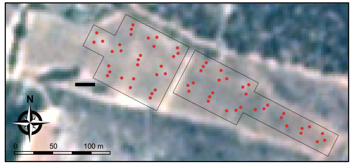
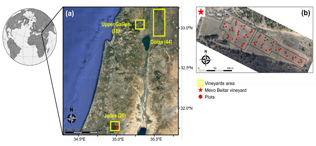
2.1. The Study Region

Our study was undertaken over 81 commercial vineyards and one experimental vineyard in Israel during the 2017 growing season. The study targeted three regions, Judea, Upper Galilee, and Golan Heights, located in hilly areas in the central and northern parts of Israel (approximately 110 km apart; Figure 1a) in which grapevines are grown in small commercial vineyards for premium high-quality wine production. All of the vineyards were subjected to a Mediterranean climate, characterized by rainfall limited to the mild winter months and hot dry summers.
In the Golan Heights region, vineyards typically consisted of cabernet sauvignon (32%), merlot (16%) and other red and white species (Table A1). Located at elevations of 600–1120 m above sea level (m.a.s.l.), these vineyards receive a mean annual rainfall amount of c. 800 mm y−1. The minimum and maximum mean air temperatures in this region during 2017 were −5.6 °C and 34.3 °C for January and August, respectively.
In the Upper Galilee, vineyards consisted of cabernet sauvignon (22%), chardonnay (17%) and other red and white species (Table A1), which were grown at elevations of 710–830 m.a.s.l. The mean annual rainfall amount in the Upper Galilee region is 670 mm y−1, with minimum and maximum mean air temperatures of −0.6 °C and 33.8 °C for January and August 2017, respectively.
In the Judea region, vineyards mainly consisted of merlot (40%), cabernet sauvignon (22%) and other red species (Table A1). Vineyards are typically located at elevation of 600–740 m.a.s.l., receiving a mean annual rainfall amount of c. 535 mm y−1. Minimum and maximum mean air temperatures in this region were 2 °C and 38.2 °C for January and August 2017, respectively.

2.2. Characteristics of the Vineyards and Irrigation Strategy

Vine spacing in the 82 vineyards was at most 1.5 m × 3 m. Soils are quite homogenous in the Golan vineyards, consisting mainly of brown alluvial soils in the northern vineyards and peat soils in the southern vineyards. In Galilee and Judea vineyards, soils are much more heterogeneous, consisting mainly of basaltic and brown terra rossa soils.
The Mevo Beitar experimental vineyard, located within the Judea region (31°43′ N; 35°06′ E; red star in Figure 1a), covers a total area of 2.4 hectares. The average elevation of the vineyard area is 700 m.a.s.l. Grapevines (Vitis vinifera L. cv. Cabernet Sauvignon) were planted in 2011 in a northwest-to-southeast direction with a vine and row spacing of 1.5 m and 3.0 m, respectively (Figure 1b). The height of the canopy typically varies between 2.0 m and 2.5 m.
Irrigation in the 82 vineyards was through a surface drip irrigation system using unilateral cordons trained to vertical shoot positioning (VSP) on a 2-m-high two-wire trellis system. The irrigation control unit was set manually to be as close as possible to the agricultural standard practice [2,35]. The irrigation strategy used in the vineyards is of deficit irrigation based on ETo (reference evapotranspiration) information provided by the Israel Meteorological Service (IMS) from a nearest IMS station to the vineyard. In practice, irrigation was applied approximately once a week, with a daily amount that ranged between 0.8 and 1.43 mm per day in Mevo Beitar. Deficit irrigation started on DOY 131 (DI start; Figure 2) and was applied throughout the season until EOS. DI ranged along the season between 14% and 25% of the vine evapotranspiration (ETc) [2], while ETc was calculated from a modified leaf area index to crop coefficient ratio for vines [36,37].
Other specific characteristics of the 81 commercial vineyards are summarized in Table A1.

2.3. Measurements of Midday Stem Water Potential in Vineyards

Measurements of Ψstem were conducted periodically by a team of agronomists hired by the growers, approximately once a week in six grapevines per vineyard in each of the 81 commercial vineyards throughout the 2017 growing season. Ψstem was measured prior to irrigation at solar noon (from 12:00 to 14:30), using a portable pressure chamber (model Arimad 2, Kfar Charuv, Israel and Arimad 3000, MRC, Hulon, Israel) according to the procedures described in [38]. Six sunlit, mature, fully expanded leaves from each vineyard were double bagged (plastic bags covered with aluminum foil) 1.5 h prior to measurement. The leaves were disconnected from the vines by sharp cutting of the leaf petiole and quickly placed in the pressure chamber. The time elapsing between leaf excision and chamber pressurization was less than 25 s. The six grapevines were selected by visual observation as representative of the entire vineyard.
At the experimental vineyard in Mevo Beitar (Figure 1a, Figure A1), we measured Ψstem in 60 plots (c. 5 m2 each) approximately every week during the 2017 growing season in order to monitor the spatial variability in Ψstem across the vineyard area. Each plot contained two grapevines (total N = 120 vines), from which 4 leaves were taken for Ψstem measurements. The Ψstem measurements in Mevo Beitar were conducted using a portable pressure chamber (Arimad 3000, MRC, Hulon, Israel), as described above.

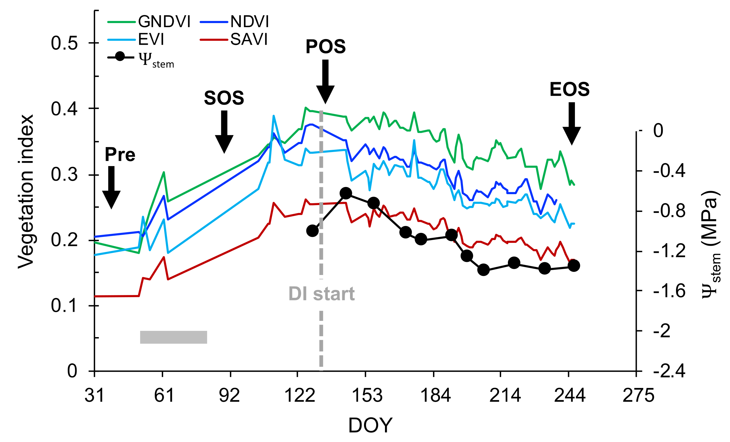
2.4. Vegetation Indices

We used four VIs in this study: the enhanced vegetation index (EVI), the soil-adjusted vegetation index (SAVI), and the abovementioned GNDVI and NDVI. These four VIs, as many others, are based on the ratio of solar reflection at the visible bands (RGB) to that at the near infrared (NIR) waveband (Table 1). The four VIs used here are regularly used in studies for tracking changes in plant-related traits, such as leaf growth (e.g., leaf area index), transpiration and evapotranspiration, as well as CO2 uptake and aboveground biomass from optical sensors mounted on unmanned aerial vehicles and/or satellites [9,17,39,40,41,42] (see also Box 1 in [32]).
Of the four VIs, NDVI is the most widely used [32]. Although NDVI has some saturation issues over dense vegetation [43], it was shown to be very reliable in monitoring vegetation dynamics, particularly in natural [8] and agricultural [16] Mediterranean vegetation systems. GNDVI, which is quite similar to NDVI, with the difference being that it uses the green instead of the red band (Table 1), is considered to be more sensitive to changes in chlorophyll-a concentrations compared to NDVI [44,45]. EVI and SAVI were both designed to overcome the saturation drawbacks in NDVI and GNDVI [43,46]. With a canopy background adjustment factor, both indices are considered to be efficient in terms of reducing soil background effects, with SAVI apparently being the most effective in that sense [43].
The four VIs were derived using the four spectral bands provided by Planet’s images following the formulations given in Table 1.

2.5. Phenological Stages

We defined here three main phenological stages, which may be observed through changes in the VI time series (Figure 2). The three stages are: start of season (SOS), which corresponds to the time when the vines started their growth around DOY 80–90 (budburst stage), approximately one month prior to the start of the irrigation; peak of season (POS), when the canopy of the vines reached their full capacity (around DOY 120–140; full bloom stage); and end of season (EOS), around DOY 240–250, the harvest stage.
Expansive understory presence in the form of volunteer weeds and grasses occurs in Israeli vineyards around DOY 50–85 prior to SOS (see in Mevo Beitar vineyard; Figure 2). This understory vegetation was treated with herbicide in most of the Galilee vineyards and mechanically removed at the end of the spring in the Golan vineyards and in most of the vineyards in the Judea region.
Finally, pre-growth season (Pre) was defined here as the time when green vegetation (including understory weeds and grasses) is absent or dry in the vineyard, at approximately DOY 30 (Figure 2).

2.6. Satellite Data

2.6.1. Planet Satellites

Planet [34] is a commercial company running a constellation of small, standardized CubeSat 3U form factor (10 × 10 × 30 cm) nano-satellites of approximately 4 kg in mass. Planet currently operates more than 175 of the so-called ‘Doves’ PlanetScope (PS) nano-satellites, providing unprecedented daily nadir-pointing high-resolution land surface imaging of the entire earth. Planet’s PS satellites provide images at a spatial resolution of 3 m (nadir ground sampling distance) in four spectral bands (RGB and NIR), with an equatorial overpass time of 9:30–11:30 a.m. (local time) [33], sometimes even three times a day (i.e., from different Doves). Planet Team currently provides a series of application programming interface (API) tools, such as Clips API [49].
In this study, a total of 3015 clipped PlanetScope Ortho Tiles were downloaded for 2017 using the Clips API for the vineyard areas within the three regions of interest (Figure 1a). Tiles were downloaded as TIFFs, often including several files for a specific date with also missing images in some dates due to cloudy conditions (<10% missing data). Figure A1 shows a true RGB color Planet image of Mevo Beitar vineyard alongside the plots where Ψstem were measured (see Section 2.3), for comparison of scales.

2.6.2. Building Time Series of Planet’s Vegetation Indices in Google Earth Engine

We used Google Earth Engine (GEE; https://earthengine.google.com/), which is a freely available cloud-based geospatial processing platform that combines a large catalog of satellite imagery and geospatial datasets with planetary-scale analysis capabilities [50]. All downloaded PS-clipped TIFFs, as well as the shapefile vector layers of the 82 vineyards (i.e., polygons), were uploaded as image- and feature collections to GEE. Then, GEE JavaScript API was used to: (1) calculate the four vegetation indices (VIs) for all images; (2) merge the number of images to a single image per date using a maximum value criteria (i.e., creating an image mosaic by selecting the maximum value for each pixel from all available images for that day) [43]. In this way, noisy data caused by cloud contamination and/or sensor view uncertainties were eliminated from the image; (3) generate time series of the four VIs; (4) calculate the time series of the averaged VI over the entire area of the vineyard (i.e., over all pixels within the vineyard area), for the 82 vineyards, and for the 60 plots within the vineyard area of Mevo Beitar (Figure 1b).

2.6.3. Time Series Analysis

To further eliminate noisy data in the time series, smoothing techniques are usually applied [32]. However, these techniques need the time series to be complete or at least have a predefined seasonal signal [51]. Because we aim at predicting Ψstem from VIs without having prior information on the seasonal behavior of the vineyard, conventional smoothing techniques could not be used. Instead, we adopted a simple weekly average approach similar to a moving average on a complete time series to eliminate noisy data. We calculated the weekly average VI value (VI avg) for each vineyard. In addition, for the time series analysis the maximum and minimum VI values in each week were extracted (VI max and VI min, respectively). To further eliminate noise of background signal related to soil and/or understory vegetation, the VI avg was scaled by dividing it by the VI avg value at POS.
Another important variable used in the time series analysis is ΔVI, which is defined as the difference between the VI avg at POS and that at Pre, when green vegetation is absent in the vineyard. This ΔVI represents the difference in fractional vegetation cover between the two periods due to leaf expansion and canopy development of the vines. This means that vineyards with vines of less developed canopies will display a small ΔVI compared to those with more developed canopies. Because Ψstem is from the vines and VI is a mixed signal from vines and background signal, we would expect a negative correlation between ΔVI and the slope of the VI–Ψstem relationship, meaning a weak VI response (steeper slope) to seasonal variations in Ψstem, in vineyards with small ΔVI (less developed canopies).

2.7. Statistical Analysis

Three models were tested in this study:
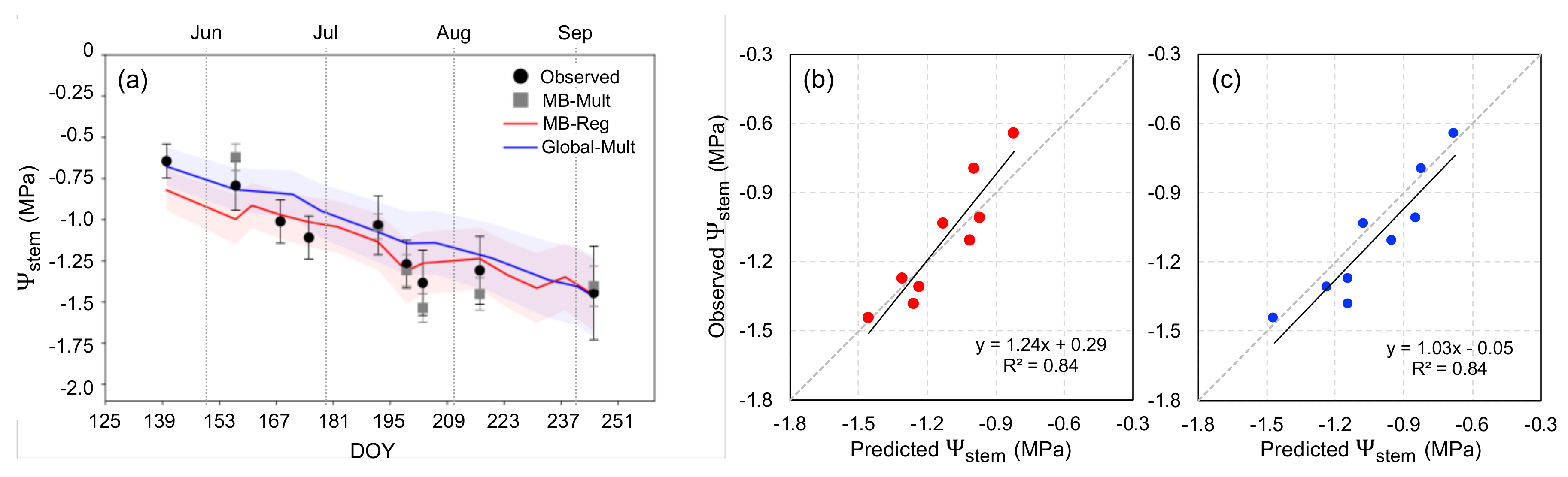
  • A multivariable linear model with five variables (VI avg, VI max, VI min, ΔVI and day of year) was used to predict weekly Ψstem (one model per week) in Mevo Beitar vineyard (hereafter, MB-Mult model).
  • A single linear regression model was used in Mevo Beitar to predict Ψstem from VIs for the entire season using the VI time series (hereafter, MB-Reg model).
  • A single ‘global’ multivariable linear model with the same variables as in MB-Mult was used to predict seasonal Ψstem from VI time series of the 81 commercial vineyards (hereafter, Global-Mult).
In Global-Mult, variables from all four VIs were first used in a single multivariable model with a total of 20 variables, five variables per VI. Then, to avoid multicollinearity issues in the model only the statistically significant variables (p < 0.05) with the highest size effect in the model were maintained, one VI per variable (total of five variables). The Global-Mult with the five variables was then used to predict Ψstem in the experimental vineyard of Mevo Beitar, comparing it with MB-Mult and MB-Reg. It should be noted that in MB-Mult and Global-Mult, the values of the variables change along the season, while the value of ΔVI remains the same.
Pearson’s r of the correlation, coefficient of determination (R2), and root square mean error (RMSE) were used as measures of model performance and to compare between the models. The size effect of each variable in Global-Mult, which is the effectiveness of the variable in predicting Ψstem, is presented as LogWorth, defined as −log10(p-value). The larger the LogWorth, the stronger is the effect of the variable in the model. All statistical analyses were carried out using JMP® software version 14.0 (SAS Institute Inc., Cary, NC, USA).

3. Results

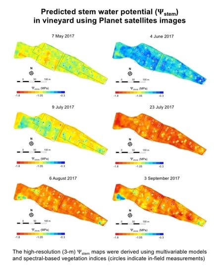
3.1. Deriving Midday Stem Water Potential for Mevo Beitar Vineyard

Figure 2 shows daily time series of the four vegetation indices alongside the Ψstem, while both VI and Ψstem were averaged over the entire vineyard area at Mevo Beitar. In general, all four VIs showed a decreasing trend similar to that of the Ψstem consequential to soil water depletion and increasing atmospheric demand for evapotranspiration. The inherent soil-background reduction capacity of SAVI is well noted in Figure 2, displaying the lowest values in comparison to the other three VIs (GNDVI, NDVI and EVI).
Low VIs values in DOYs 30–50 (Pre stage) are related mainly to soil background and dry understory vegetation. Peak VI at POS is from the fully developed canopies of the vines at this time of the season, at the start of the irrigation.
MB-Reg was significant for all four VIs (p < 0.01), with r = 0.80–0.82 (Figure 3). High VI values were generally associated with less negative Ψstem at the time when DI started, while low VI values were associated with more negative Ψstem, reflecting the water stress condition of the vines towards EOS (DOY 245).
Table 2 summarizes the statistics of MB-Mult for the four VIs. Here, again, SAVI showed a better performance than the other three indices, likely due to its higher capacity in reducing soil background effects. GNDVI, NDVI and EVI show quite similar r scores, with NDVI showing a slightly better performance than GNDVI and EVI (Table 2). The highest r scores were mostly obtained from DOY 189 towards EOS (DOY 245), although with a generally higher RMSE as well.
With the exception of one week (DOY 168), models were generally statistically significant along the season with an average r score > 0.64 (Table 2). It should be noted, though, that the week corresponding to DOY 168 was particularly cloudy, which likely affected Planet-derived VI and consequently the MB-Mult models in this particular week.
Figure 4 shows high-resolution maps of Ψstem in Mevo Beitar vineyard from MB-Mult using SAVI for selected dates. The spatial pattern of Ψstem varies throughout the growing season (Figure 4). Ψstem in DOY 154 was relatively high across the vineyard compared to other dates because of the DI start in DOY 131 (Figure 2) and the relatively lower atmospheric demand compared to the following weeks.
Figure 5 shows the difference (ΔΨ) between the Ψstem derived from MB-Reg and MB-Mult (both using SAVI). ΔΨ in Figure 5 was calculated as the absolute Ψstem value from MB-Reg minus the absolute Ψstem value from MB-Mult. Thus, blue colors indicate lower values of Ψstem (more stressed) in MB-Reg than in MB-Mult, while red colors mean that Ψstem was higher (less stressed) in MB-Reg than in MB-Mult. Most of the maps in Figure 5 show a uniform distribution of ∆Ψ across the vineyard, which means that MB-Reg was able to reproduce the spatial variability in Ψstem close to that predicted by MB-Mult, though with some differences in magnitude. Yet, at both ends of the growing season, before and after the DI start (DOY 126 and 245), ∆Ψ across the vineyard shows a significant spatial variability.
These results indicate that the measures from both models are consistent with one another for much of the season. Thus, for irrigation management, either approach could be used to monitor relative difference (spatial variability) within the field at Mevo Beitar, to the extent that such information could be used to improve the efficiency of ground operations.

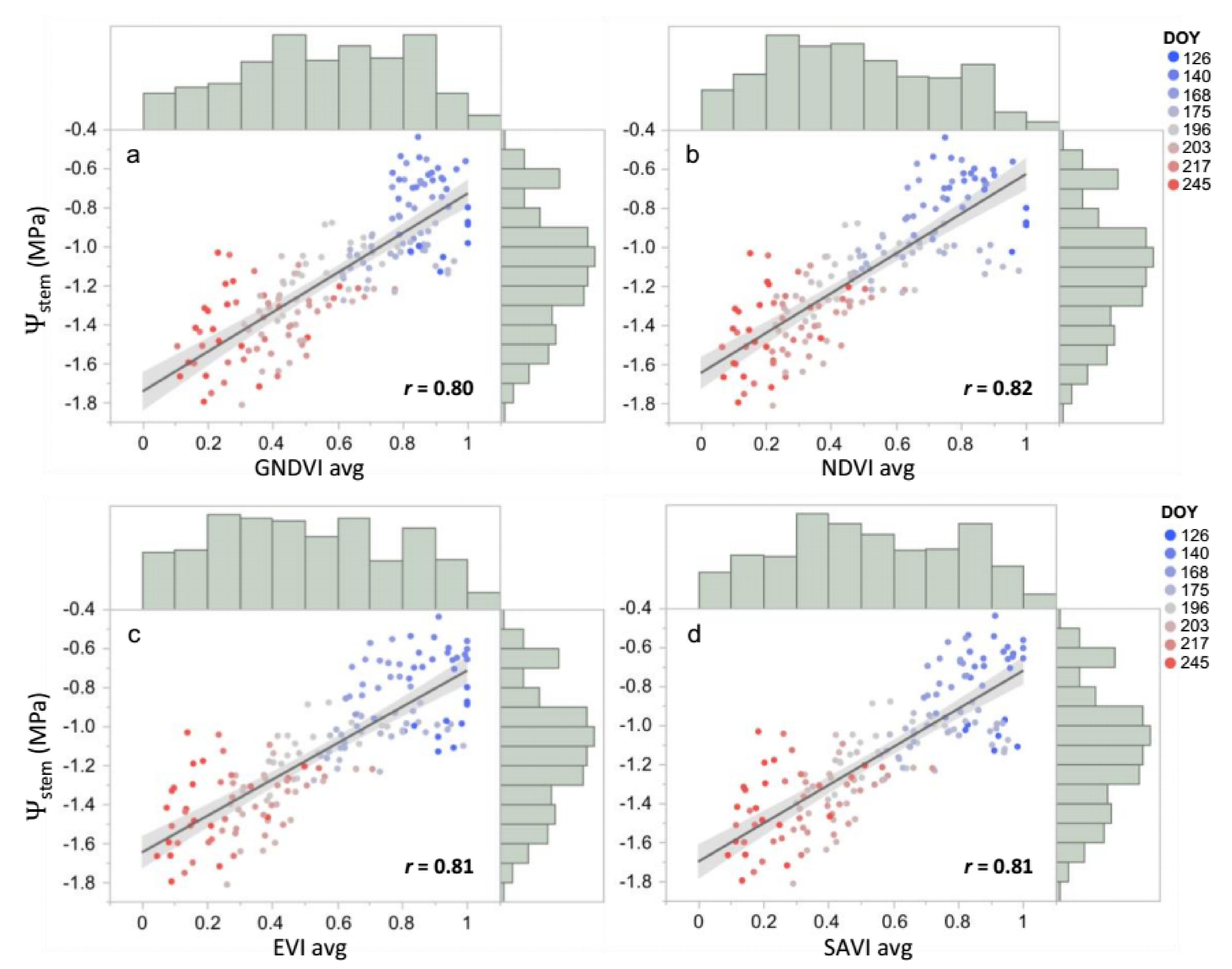
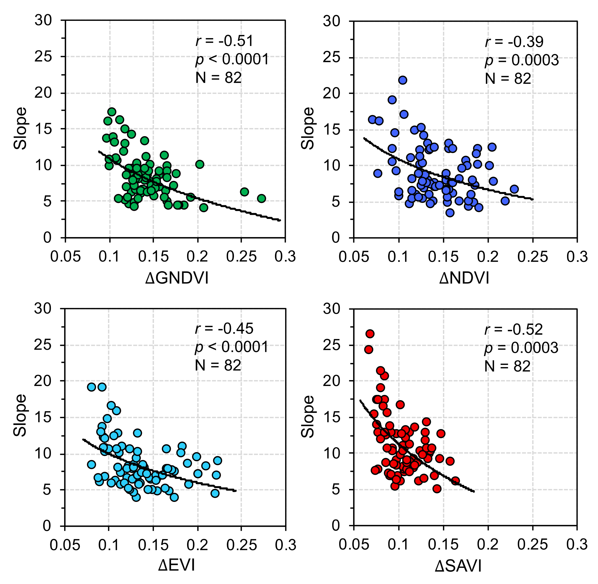
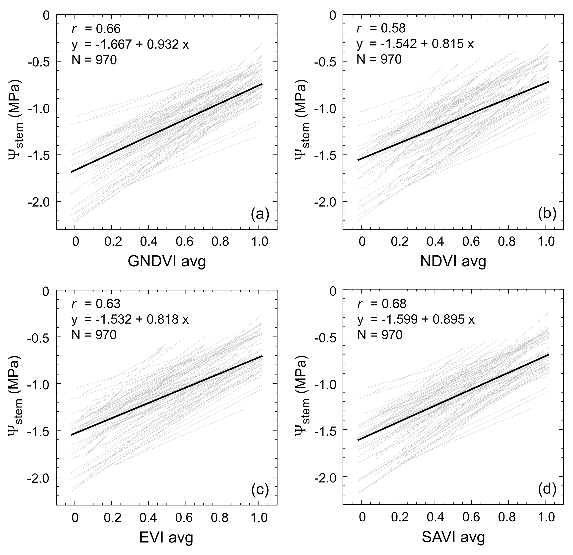
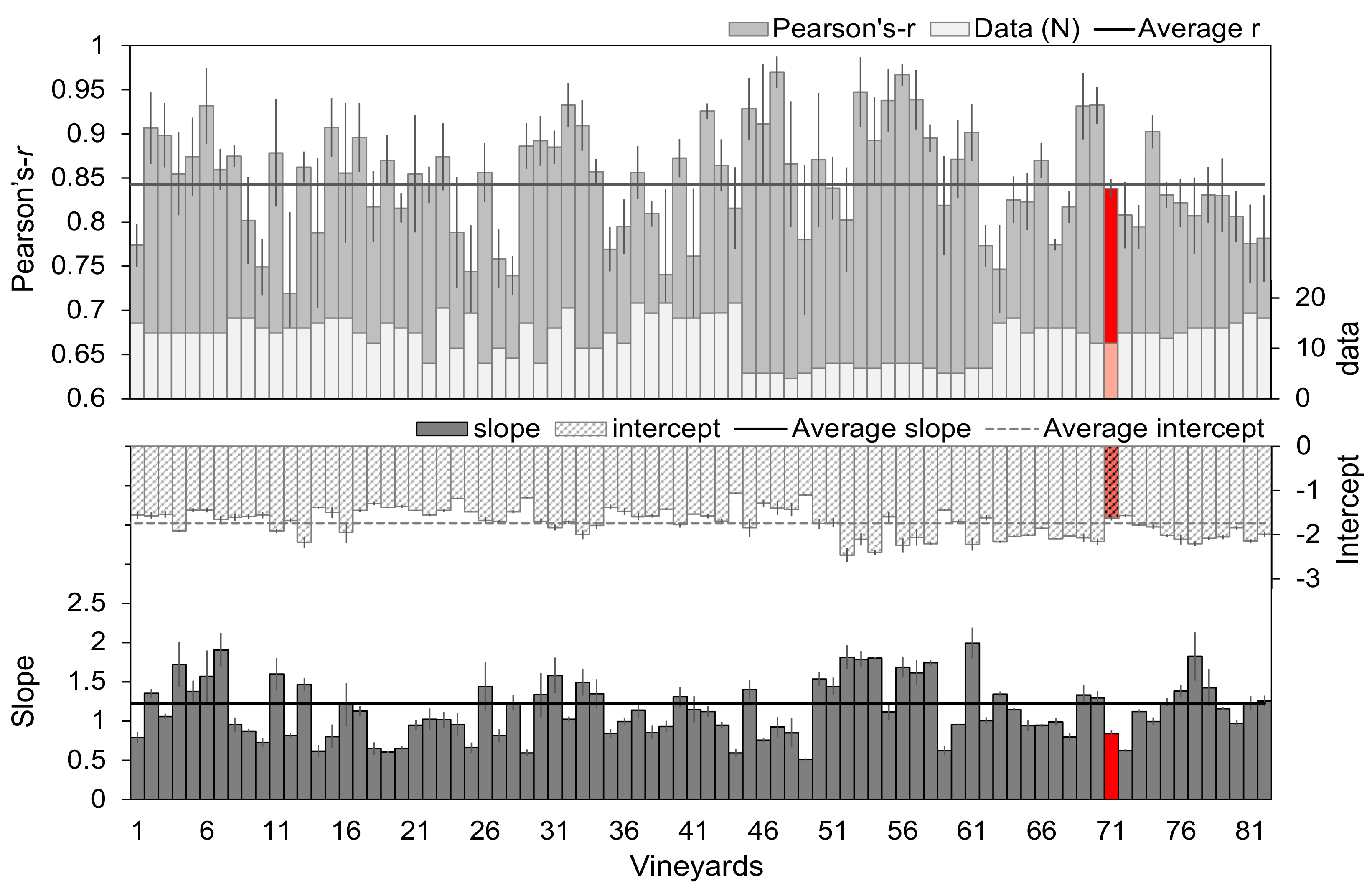
3.2. Vegetation Indices and Stem Water Potential in Vineyards across Rainfall Gradient

The Pearson’s r of the VI-Ψstem linear fit using all data from the 82 vineyards together was positive and significant (p < 0.001), with 0.58 < r < 0.68 for the four VIs (Figure 6). Once again, SAVI was demonstrated to be the most successful index in tracking seasonal changes in Ψstem in the 82 vineyards (Figure 6d).
The per-vineyard Pearson’s r of the VI-Ψstem linear fits ranged between 0.72 and 0.97, with an average r of 0.85 ± 0.06 (Figure 7). Linear fits, though, differed between vineyards in terms of intercept and particularly in slope (Figure 6 and Figure 7).
Background effects of soil and/or understory vegetation were likely responsible for the different slopes of the linear fits (Figure 6 and Figure 7). Vineyards with a large background effect had more pronounced slopes, meaning weak VI response to seasonal changes in Ψstem. This background effect may be noted as a negative correlation between ΔVI and the slope of the VIs-Ψstem linear fit in Figure 8.
Figure 8 shows that for vineyards with a small ΔVI (weak VI response to Ψstem change), or, in other words, with grapevines of less developed canopies and thus a larger background effect, the slope of the VIs-Ψstem linear fit was steeper than for vineyards with a large ΔVI. This suggests that ΔVI is an important variable in predicting Ψstem and may assist in distinguishing between vineyards with different levels of background effect.
The performance of each of the four VIs in a multivariable regression model (one model per VI) was quite similar (r = 0.76, for the four VIs), with a slight improvement (r = 0.78; RMSE = 18.5%; Figure 9) when using variables from different VIs in Global-Mult (Table 3). Global-Mult, though, was a significant improvement over the simple linear regression model used with the VI time series (0.58 < r < 0.68, Figure 6).
As for the size effect (LogWorth) of each variable in the model, DOY was the one with the strongest effect (Table 3). The variable with the next-strongest effect was ΔNDVI, meaning a strong background effect in the vineyards, as already suggested by the relationship shown in Figure 8. The SAVI avg had also a significant effect, comparable to the size effect of ΔNDVI (Table 3).

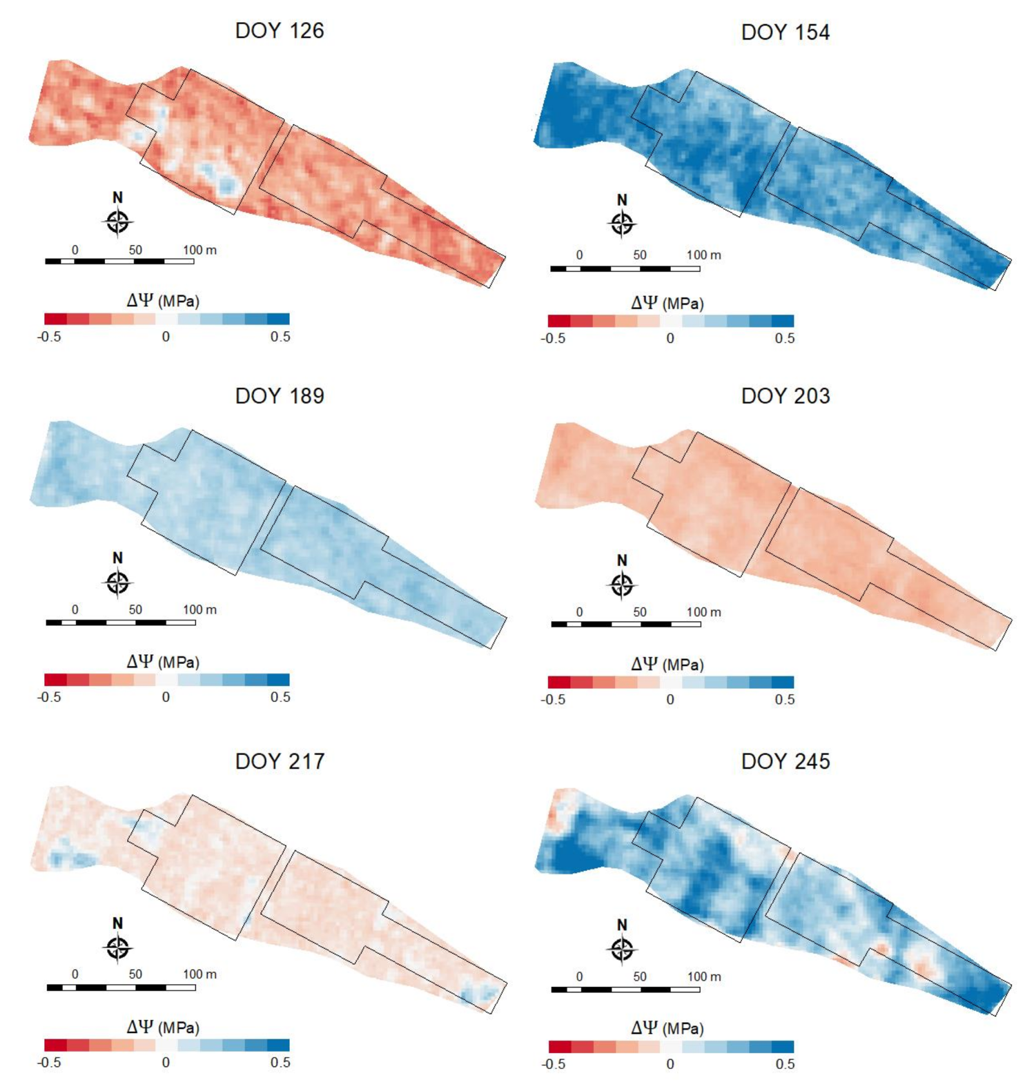
3.3. Predicting Stem Water Potential at Mevo Beitar Vineyard Using Single ‘Global’ Model

Figure 10 shows the comparison between measured Ψstem averaged over the 60 plots at Mevo Beitar vineyard during the season of 2017 and predicted Ψstem using MB-Reg, MB-Mult and Global-Mult.
Global-Mult is shown to reproduce seasonal changes in observed Ψstem at Mevo Beitar with a fairly high accuracy (R2 = 0.84; RMSE = 0.12; bias = 0.07, Figure 10a,c), at least as good as the site-specific models of MB-Reg (R2 = 0.84; RMSE = 0.11; bias = −0.02, Figure 10a,b) and MB-Mult (Figure 10a). Thus, Global-Mult appears to present a useful tool for seasonal (weekly) predictions of Ψstem in Mediterranean vineyards.

4. Discussion

Management of spatial variability within a vineyard can increase profits significantly by allowing optimization of yield quantity and quality [52,53]. Technologies and methodologies are currently being developed to allow variable-rate irrigation in drip irrigated vineyards and orchards [54,55]. Since the current state of the art for irrigation decision-making uses time- and labor-consuming measurement of Ψstem [2,35,36,56], remote sensing methodologies successfully acting as stem water potential proxies have particular appeal. That said, there remains a challenge in finding remotely acquired data that: (a) has sufficiently reliable correlation with Ψstem, (b) is affordable and accessible, and (c) has both high spatial and temporal resolution, each of which are necessary in order for the method to be useful for high frequency irrigation scheduling.
This study showed a significant correlation between vegetation indices derived from high-resolution Planet images (3-m) and Ψstem in Mediterranean (Israel) vineyards. Previous studies have shown that CWSI and NIR-based indices, like GNDVI and NDVI, may be good indicators of water status in grapevines through correlations with leaf stomatal conductance (gs) and water potential (ΨLeaf and Ψstem). However, these relationships were mostly observed at the canopy- [22,28,29] or leaf [30,31] levels using manual spectroradiometers or sensors mounted on small airplanes and drones. As far as the authors are aware, this is the first study that shows such a relationship using images of coarser spatial resolution acquired from satellites, and more specifically from Planet nano-satellites.
One of the main challenges when using satellite information is the spatial resolution of the images, which is often coarser than the targeted object and may induce a mixed-pixel signal effect. For example, understory vegetation was shown to affect satellite spectral signals in complex vegetation systems comprised of multi-canopy layers [32]. The multi-canopy layer, vertical mixed-pixel effect was further corroborated in a simulation model by Chen et al. [57], implying that understory vegetation may significantly affect satellite signals. In our case, understory expansion reaches its maximum at ~DOY 60, while vines budburst occurs later at DOY 80–90. Background effect in the vineyards, which may include the signal from soil and/or understory vegetation, was observed through a different VI-Ψstem linear fit in terms of magnitude of slope (slope ranged between 0.5 and 2), meaning that some vineyards experienced weak VI response to seasonal changes in Ψstem, while others experienced a stronger response to Ψstem changes. This differential response is due to the fact that in vineyards with grapevines of more developed canopies, and consequently less exposed understory cover seen from the satellite, the VI signal is mostly coming from the vines while in vineyards with less developed vines much of the VI signal comes from the ground.
To overcome this mixed-pixel effect, we used the difference between the VI signal at the POS, which corresponded mainly to the grapevines, and that of the understory derived at the Pre (ΔVI). That way, background effects were eliminated allowing vineyards with diverse soil and understory vegetation characteristics to be compared and used in a single ‘global’ model. Results from the Global-Mult model showed that ΔNDVI had a significant size effect, being a key factor in predicting Ψstem, with only day of year having a stronger size effect and SAVI avg a similar effect (Table 3).
In Mevo Beitar, a highly variable vineyard, weekly based correlations (Pearson’s r) of GNDVI, NDVI, EVI and SAVI vs. Ψstem were within the range of 0.28–0.84, with an average value of 0.65 for all indices (Table 2). These results were quite similar to previously reported VI-Ψstem correlations found by others using very-high-resolution images [22,29]. When time series were used in the regression instead of date-specific data, correlations were even higher (0.80 < r < 0.82). A simple linear regression model (MB-Reg) was sufficient to reproduce temporal, as well as spatial variations in Ψstem in the experimental vineyard.
In general, correlations from simple specific-date regressions between vegetation indices and Ψstem were also high for the 81 commercial vineyards (r = 0.72–0.97; Figure 7), implying that Planet-derived time series of vegetation indices like, GNDVI, NDVI, EVI and SAVI may be good indicators of water status at the vineyard-scale level.
Finally, the Global-Mult model with spectral-based indices derived from Planet satellites was proposed to predict Ψstem in Mediterranean vineyards. After deriving ΔNDVI, SAVI avg, NDVI max and NDVI min of a specific vineyard a real-time Ψstem estimation may be provided for that vineyard at a weekly basis. The Global-Mult shows promise in improving the efficiency of in-field conventional monitoring efforts.

5. Conclusions

The relationship between stem water potential and vegetation indices was evaluated in Mediterranean vineyards through the use of high spatial resolution Planet nano-satellite imaging on the freely available GEE cloud computing system for the first time. Using JavaScript API in GEE allowed fast computation of the derivation of time series of vegetation indices for the area of the 82 vineyards, showing potentials for real-time monitoring in small-size agricultural fields.
The four vegetation indices tested in this study (GNDVI, NDVI, EVI and SAVI) showed significant correlation with stem water potential, with SAVI displaying a slightly better performance, likely due to its capacity for reducing soil effects. Correlations using of the four vegetation indices were high for measurements across the vineyard area (0.89 < r < 0.82 for MB-Reg and 0.64 < r < 0.67 for MB-Mult) and along the season (r = 0.92 for both MB-Reg and Global-Mult), allowing predictions of stem water potential variability in space and time.
A method to reduce the background effect of understory vegetation and soil, which accounts for the fractional cover of the vines, was also presented. The fractional cover of the vines was retrieved as the difference in the value of the vegetation index at the peak of season and prior to the appearance of green vegetation in the vineyard (ΔVI). This ΔVI, was negatively correlated with the slope of the vegetation index to stem water potential relationship, meaning that vineyards with a low fractional cover have weak VI response to changes in measured stem water potential. Using the ΔVI allowed the development of a ‘global’ multivariable model for predicting stem water potential in vineyards with different background (soil and understory presence) characteristics.
Overall, the approach presented here shows promise in exploiting these technologies, which include resolving the mixed-pixel problem in agricultural as well as in the ecological monitoring of natural vegetation systems from satellites. The tools developed here, i.e., the combination of Planet images and GEE platform, with the aforementioned mixed-pixel separation approach, may be also used for water status monitoring of agricultural fields other than vineyards.
Finally, pending further verification and validation, the proposed ‘global’ model presented here may be used for real-time irrigation management along the season from the abovementioned weekly values extracted using daily Planet images. Using the ‘global’ model could substantially improve sampling efficiency of conventional water status monitoring. The methodology developed in this study should be further examined with supporting information on soil texture, LAI/fractional cover and understory vegetation. Moreover, a comparison with freely available satellite images like those from Sentinel-2, which have coarser spatial (10–20 m) and temporal (5 day) resolution than Planet, should be conducted.

Author Contributions

Conceptualization, D.H. and Y.C.; Data curation, A.P.; Formal analysis, D.H.; Funding acquisition, A.B.-G., V.A. and Y.C.; Investigation, D.H., I.B., Y.N., A.B.-G., A.P. and Y.C.; Methodology, D.H.; Project administration, V.A. and Y.C.; Resources, I.B., A.B.-G., V.A. and Y.C.; Software, D.H.; Supervision, Y.C.; Validation, D.H., I.B. and Y.N.; Visualization, D.H.; Writing—original draft, D.H.; Review & editing, D.H., Y.C., Y.N., I.B., A.B.-G., A.P. and V.A.

Funding

This research was funded by the Chief Scientist Fund of the Ministry of Agriculture and Rural Development in Israel, grant number [20-12-0030].

Acknowledgments

The authors thank Itamar Lensky for fruitful discussions, Yaron Michael and Shilo Shif for assisting with GEE Java script and Planet’s Clip API, and Planet Labs for providing API tools and images, as part of Planet’s Education and Research Program. We also thank Ben Hazut, for assistance in the field and laboratory, Yair Hayat from Barken Winery, Shlomo Zsadok and Tamar Sokolsky from Golan Heights Winery, David Twito and Dror Dotan from Carmel wineries for agro-technical assistance. This research was supported by the Chief Scientist Fund of the Ministry of Agriculture and Rural Development in Israel (Grant No. 20-12-0030).

Conflicts of Interest

The authors declare no conflict of interest. The funders had no role in the design of the study; in the collection, analyses, or interpretation of data; in the writing of the manuscript, and in the decision to publish the results.

Appendix A

Figure A1. A true RGB color Planet image (from 3 June 2016) of Mevo Beitar vineyard with location of the 60 Ψstem measurement plots.
Remotesensing 10 01615 g0a1
Table A1. General characteristics of the 82 vineyards used in this study. The region, size of the vineyard (in hectares) and species are shown alongside the minimum (most negative) seasonal Ψstem (MPa) in the vineyard and the DI start and EOS dates. In bold is Mevo Beitar vineyard.
#RegionSize (ha)SpeciesRed/WhiteΨstem (MPa)DI StartEOS
1Golan1.74Cabernet Francred−1.37614-May27-Aug
2Golan1.34Chardonnaywhite−1.72128-May10-Sep
3Golan0.95Chardonnaywhite−1.51828-May10-Sep
4Golan1.30Cabernet Sauvignonred−1.80628-May10-Sep
5Golan0.85Cabernet Sauvignonred−1.50028-May10-Sep
6Golan0.70Cabernet Sauvignonred−1.42728-May10-Sep
7Golan1.16Cabernet Sauvignonred−1.74328-May10-Sep
8Golan1.00Cabernet Sauvignonred−1.54314-May05-Sep
9Golan1.42Cabernet Sauvignonred−1.53314-May05-Sep
10Golan2.07Merlotred−1.43214-May14-Aug
11Golan1.30Petit Verdotred−1.72928-May10-Sep
12Golan1.81Syrared−1.58314-May13-Aug
13Golan1.13Syrared−1.44514-May14-Aug
14Golan1.30Chardonnaywhite−1.34029-May11-Sep
15Golan1.21Chardonnaywhite−1.33829-May11-Sep
16Golan2.13Chardonnaywhite−1.55629-May11-Sep
17Golan3.13Chardonnaywhite−1.48529-May11-Sep
18Golan0.84Cabernet Sauvignonred−1.50405-Jun03-Sep
19Golan1.47Cabernet Sauvignonred−1.36629-May11-Sep
20Golan1.77Cabernet Sauvignonred−1.55029-May11-Sep
21Golan1.36Pinot Griswhite−1.46329-May04-Sep
22Golan1.98Cabernet Sauvignonred−1.48622-May07-Sep
23Golan2.42Cabernet Sauvignonred−1.54523-May18-Sep
24Golan2.11Cabernet Sauvignonred−1.16105-Jun07-Sep
25Golan2.05Merlotred−1.63829-May18-Sep
26Golan1.58Merlotred−1.41025-Jun10-Sep
27Golan0.96Merlotred−1.56825-Jun07-Sep
28Golan3.88Merlotred−1.62112-Jun10-Sep
29Golan1.17Petit Verdotred−1.25813-Jun18-Sep
30Golan2.39Sauvignon Blancwhite−1.51119-Jun23-Aug
31Golan0.87Syrared−1.80706-Jun05-Sep
32Golan0.96Syrared−1.76523-May18-Sep
33Golan1.22Syrared−1.80705-Jun31-Aug
34Golan3.60Syrared−1.55412-Jun16-Aug
35Golan2.51Viognierwhite−1.36815-May31-Aug
36Golan2.36Viognierwhite−1.52015-May07-Sep
37Golan0.76Cabernet Sauvignonred−1.47908-May11-Sep
38Golan2.60Cabernet Sauvignonred−1.54019-May11-Sep
39Golan1.56Malbecred−1.46908-May11-Sep
40Golan1.98Merlotred−1.60119-May11-Sep
41Golan2.77Merlotred−1.41919-May11-Sep
42Golan3.98Sangiovesered−1.58119-May11-Sep
43Golan1.52Syrared−1.71219-May11-Sep
44Golan1.00Tinta Caored−1.10408-May11-Sep
45Galilee2.97Cabernet Francred−1.27010-May18-Jul
46Galilee1.35Petit Syrared−1.00910-May18-Jul
47Galilee2.95Viognierwhite−1.07310-May18-Jul
48Galilee1.81Malbecred−1.15110-May18-Jul
49Galilee2.99Chardonnaywhite−0.86910-May18-Jul
50Galilee2.54Chardonnaywhite−1.19502-May29-Aug
51Galilee2.64Muscat Caneliwhite−1.48602-May29-Aug
52Galilee3.84Merlotred−1.43102-May29-Aug
53Galilee2.87Viognierwhite−1.35602-May15-Aug
54Galilee3.59Chardonnaywhite−1.44102-May15-Aug
55Galilee4.81Roussannewhite−1.19606-Jun29-Aug
56Galilee3.67Cabernet Sauvignonred−1.59406-Jun29-Aug
57Galilee4.26Cabernet Sauvignonred−1.53606-Jun29-Aug
58Galilee3.35Gewurztraminerwhite−1.24602-Jun15-Aug
59Galilee3.65Pinot Noirred−1.24324-May16-Aug
60Galilee3.06Tannatred−1.52824-May16-Aug
61Galilee5.46Cabernet Sauvignonred−1.77024-May30-Aug
62Galilee2.43Cabernet Sauvignonred−1.61124-May30-Aug
63Judea1.43Merlotred−1.98915-May11-Sep
64Judea1.28Cabernet Sauvignonred−1.96129-May11-Sep
65Judea1.83Cabernet Sauvignonred−1.75814-May20-Aug
66Judea1.08Petit Verdotred−1.62414-May20-Aug
67Judea1.23Syrared−1.82614-May20-Aug
68Judea1.13Syrared−1.79914-May20-Aug
69Judea0.49Merlotred−1.92815-May28-Aug
70Judea0.73Merlotred−1.92815-May28-Aug
71Judea2.40Cabernet Sauvignonred−1.40010-May05-Sep
72Judea1.27Cabernet Sauvignonred−1.51414-May27-Aug
73Judea1.27Cabernet Sauvignonred−1.56614-May27-Aug
74Judea1.18Cabernet Sauvignonred−1.59314-May27-Aug
75Judea0.73Merlotred−1.67514-May13-Aug
76Judea0.55Malbecred−1.77321-May27-Aug
77Judea0.63Merlotred−2.23215-May28-Aug
78Judea0.89Merlotred−1.84015-May28-Aug
79Judea1.55Merlotred−1.92615-May28-Aug
80Judea2.01Cabernet Sauvignonred−1.79215-May11-Sep
81Judea1.26Cabernet Sauvignonred−2.02122-May11-Sep
82Judea1.39Cabernet Sauvignonred−1.92815-May11-Sep

References

  1. Ruiz-Sanchez, M.C.; Domingo, R.; Castel, J.R. Deficit irrigation in fruit trees and vines in Spain. Span. J. Agric. Res. 2010, 8, 5–20. [Google Scholar] [CrossRef]
  2. Munitz, S.; Netzer, Y.; Schwartz, A. Sustained and regulated deficit irrigation of field-grown Merlot grapevines. Aust. J. Grape Wine Res. 2017, 23, 87–94. [Google Scholar] [CrossRef]
  3. Myburgh, P.; Cornelissen, M.; Southey, T. Interpretation of Stem Water Potential Measurements. WineLand. 2016, pp. 78–80. Available online: http://www.wineland.co.za/interpretation-of-stem-water-potential-measurements/ (accessed on 15 July 2018).
  4. Mulla, D.J. Twenty five years of remote sensing in precision agriculture: Key advances and remaining knowledge gaps. Biosyst. Eng. 2013, 114, 358–371. [Google Scholar] [CrossRef]
  5. Gebbers, R.; Adamchuk, V.I. Precision Agriculture and Food Security. Science 2010, 327, 828–831. [Google Scholar] [CrossRef] [PubMed]
  6. Matese, A.; Baraldi, R.; Berton, A.; Cesaraccio, C.; Di Gennaro, F.S.; Duce, P.; Facini, O.; Mameli, G.M.; Piga, A.; Zaldei, A. Estimation of Water Stress in Grapevines Using Proximal and Remote Sensing Methods. Remote Sens. 2018, 10, 114. [Google Scholar] [CrossRef]
  7. Meron, M.; Tsipris, J.; Orlov, V.; Alchanatis, V.; Cohen, Y. Crop water stress mapping for site-specific irrigation by thermal imagery and artificial reference surfaces. Precis. Agric. 2010, 11, 148–162. [Google Scholar] [CrossRef]
  8. Helman, D.; Lensky, I.M.; Tessler, N.; Osem, Y. A phenology-based method for monitoring woody and herbaceous vegetation in mediterranean forests from NDVI time series. Remote Sens. 2015, 7, 12314–12335. [Google Scholar] [CrossRef]
  9. Helman, D.; Lensky, I.M.; Osem, Y.; Rohatyn, S.; Rotenberg, E.; Yakir, D. A biophysical approach using water deficit factor for daily estimations of evapotranspiration and CO2 uptake in Mediterranean environments. Biogeosciences 2017, 14, 3909–3926. [Google Scholar] [CrossRef]
  10. Helman, D.; Osem, Y.; Yakir, D.; Lensky, I.M. Relationships between climate, topography, water use and productivity in two key Mediterranean forest types with different water-use strategies. Agric. For. Meteorol. 2017, 232, 319–330. [Google Scholar] [CrossRef]
  11. Helman, D.; Lensky, I.M.; Yakir, D.; Osem, Y. Forests growing under dry conditions have higher hydrological resilience to drought than do more humid forests. Glob. Chang. Biol. 2017, 23, 2801–2817. [Google Scholar] [CrossRef] [PubMed]
  12. Rotbart, N.; Schmilovitch, Z.; Cohen, Y.; Alchanatis, V.; Erel, R.; Ignat, T.; Shenderey, C.; Dag, A.; Yermiyahu, U. Estimating olive leaf nitrogen concentration using visible and near-infrared spectral reflectance. Biosyst. Eng. 2013, 114, 426–434. [Google Scholar] [CrossRef]
  13. Nigon, T.J.; Mulla, D.J.; Rosen, C.J.; Cohen, Y.; Alchanatis, V.; Knight, J.; Rud, R. Hyperspectral aerial imagery for detecting nitrogen stress in two potato cultivars. Comput. Electron. Agric. 2015, 112, 36–46. [Google Scholar] [CrossRef]
  14. Di Gennaro, S.F.; Battiston, E.; Di Marco, S.; Facini, O.; Matese, A.; Nocentini, M.; Palliotti, A.; Mugnai, L. Unmanned Aerial Vehicle (UAV)-based remote sensing to monitor grapevine leaf stripe disease within a vineyard affected by esca complex. Phytopathol. Mediterr. 2016, 55, 262–275. [Google Scholar]
  15. Mahlein, A.-K. Plant Disease Detection by Imaging Sensors—Parallels and Specific Demands for Precision Agriculture and Plant Phenotyping. Plant Dis. 2015, 100, 241–251. [Google Scholar] [CrossRef]
  16. Bonfil, D.J. Wheat phenomics in the field by RapidScan: NDVI vs. NDRE. Isr. J. Plant Sci. 2017, 9978, 1–14. [Google Scholar] [CrossRef]
  17. Manfreda, S.; McCabe, M.; Miller, P.; Lucas, R.; Madrigal, V.P.; Mallinis, G.; Dor, E.B.; Helman, D.; Estes, L.; Ciraolo, G.; et al. On the use of Unmanned Aerial Systems for environmental monitoring. Remote Sens. 2018, 10, 641. [Google Scholar] [CrossRef]
  18. Khanal, S.; Fulton, J.; Shearer, S. An overview of current and potential applications of thermal remote sensing in precision agriculture. Comput. Electron. Agric. 2017, 139, 22–32. [Google Scholar] [CrossRef]
  19. Cohen, Y.; Alchanatis, V.; Saranga, Y.; Rosenberg, O.; Sela, E.; Bosak, A. Mapping water status based on aerial thermal imagery: Comparison of methodologies for upscaling from a single leaf to commercial fields. Precis. Agric. 2017, 18, 801–822. [Google Scholar] [CrossRef]
  20. Rud, R.; Cohen, Y.; Alchanatis, V.; Levi, A.; Brikman, R.; Shenderey, C.; Heuer, B.; Markovitch, T.; Dar, Z.; Rosen, C.; et al. Crop water stress index derived from multi-year ground and aerial thermal images as an indicator of potato water status. Precis. Agric. 2014, 15, 273–289. [Google Scholar] [CrossRef]
  21. Jackson, R.D.; Idso, S.B.; Reginato, J.R.; Pinter, J.P. Canopy temperature as a crop water stress indicator. Water Resour. Res. 1981, 17, 1133–1138. [Google Scholar] [CrossRef]
  22. Baluja, J.; Diago, M.P.; Balda, P.; Zorer, R.; Meggio, F.; Morales, F.; Tardaguila, J. Assessment of vineyard water status variability by thermal and multispectral imagery using an unmanned aerial vehicle (UAV). Irrig. Sci. 2012, 30, 511–522. [Google Scholar] [CrossRef] [Green Version]
  23. Bellvert, J.; Zarco-Tejada, P.J.; Girona, J.; Fereres, E. Mapping crop water stress index in a ‘Pinot-noir’ vineyard: Comparing ground measurements with thermal remote sensing imagery from an unmanned aerial vehicle. Precis. Agric. 2014, 15, 361–376. [Google Scholar] [CrossRef]
  24. Santesteban, L.G.; Di Gennaro, S.F.; Herrero-Langreo, A.; Miranda, C.; Royo, J.B.; Matese, A. High-resolution UAV-based thermal imaging to estimate the instantaneous and seasonal variability of plant water status within a vineyard. Agric. Water Manag. 2017, 183, 49–59. [Google Scholar] [CrossRef]
  25. Gutiérrez, S.; Diago, M.P.; Fernández-Novales, J.; Tardaguila, J. Vineyard water status assessment using on-the-go thermal imaging and machine learning. PLoS ONE 2018, 13, e0192037. [Google Scholar] [CrossRef] [PubMed]
  26. Möller, M.; Alchanatis, V.; Cohen, Y.; Meron, M.; Tsipris, J.; Naor, A.; Ostrovsky, V.; Sprintsin, M.; Cohen, S. Use of thermal and visible imagery for estimating crop water status of irrigated grapevine. J. Exp. Bot. 2007, 58, 827–838. [Google Scholar] [CrossRef] [PubMed]
  27. Gonzalez-Dugo, V.; Zarco-Tejada, P.; Nicolás, E.; Nortes, P. A.; Alarcón, J. J.; Intrigliolo, D. S.; Fereres, E. Using high resolution UAV thermal imagery to assess the variability in the water status of five fruit tree species within a commercial orchard. Precis. Agric. 2013, 14, 660–678. [Google Scholar] [CrossRef]
  28. Espinoza, C.Z.; Khot, L.R.; Sankaran, S.; Jacoby, P.W. High Resolution Multispectral and Thermal Remote Sensing-Based Water Stress Assessment in Subsurface Irrigated Grapevines. Remote Sens. 2017, 9, 961. [Google Scholar] [CrossRef]
  29. Zarco-Tejada, P.J.; González-Dugo, V.; Williams, L.E.; Suárez, L.; Berni, J.A.J.; Goldhamer, D.; Fereres, E. A PRI-based water stress index combining structural and chlorophyll effects: Assessment using diurnal narrow-band airborne imagery and the CWSI thermal index. Remote Sens. Environ. 2013, 138, 38–50. [Google Scholar] [CrossRef] [Green Version]
  30. Rodríguez-Pérez, J.R.; Riaño, D.; Carlisle, E.; Ustin, S.; Smart, D.R. Evaluation of hyperspectral reflectance indexes to detect grapevine water status in vineyards. Am. J. Enol. Vitic. 2007, 58, 302–317. [Google Scholar]
  31. Maimaitiyiming, M.; Ghulam, A.; Bozzolo, A.; Wilkins, J.L.; Kwasniewski, M.T. Early Detection of Plant Physiological Responses to Different Levels of Water Stress Using Reflectance Spectroscopy. Remote Sens. 2017, 9, 745. [Google Scholar] [CrossRef]
  32. Helman, D. Land surface phenology: What do we really ‘see’ from space? Sci. Total Environ. 2018, 618, 665–673. [Google Scholar] [CrossRef] [PubMed]
  33. Houborg, R.; McCabe, F.M. High-Resolution NDVI from Planet’s Constellation of Earth Observing Nano-Satellites: A New Data Source for Precision Agriculture. Remote Sens. 2016, 8, 768. [Google Scholar] [CrossRef]
  34. Planet. Planet Satellite Imagery Products. 2018. Available online: https://www.planet.com/docs/spec-sheets/sat-imagery/ (accessed on 15 July 2018).
  35. Munitz, S.; Netzer, Y.; Shetin, I.; Schwartz, A. Water availability dynamics have long-term effects on mature stem structure in Vitis vinifera. Am. J. Bot. 2018, 105. [Google Scholar] [CrossRef] [PubMed]
  36. Netzer, Y.; Yao, C.; Shenker, M.; Bravdo, B.-A.; Schwartz, A. Water use and the development of seasonal crop coefficients for Superior Seedless grapevines trained to an open-gable trellis system. Irrig. Sci. 2009, 27, 109–120. [Google Scholar] [CrossRef]
  37. Munitz, S.; Schwartz, A.; Netzer, Y. Evaluation of Seasonal Water Use and Crop Coefficients for Cabernet Sauvignon Grapevines as the Base for Skilled regulated irrigation. Acta Hortic. 2016, IV, 33–40. [Google Scholar] [CrossRef]
  38. Boyer, J.S. Measuring the Water Status of Plants and Soils; Academic Press, Inc.: San Diego, CA, USA, 1995. [Google Scholar]
  39. Helman, D.; Givati, A.; Lensky, I.M. Annual evapotranspiration retrieved from satellite vegetation indices for the eastern Mediterranean at 250 m spatial resolution. Atmos. Chem. Phys. 2015, 15, 12567–12579. [Google Scholar] [CrossRef]
  40. Candiago, S.; Remondino, F.; De Giglio, M.; Dubbini, M.; Gattelli, M. Evaluating Multispectral Images and Vegetation Indices for Precision Farming Applications from UAV Images. Remote Sens. 2015, 7, 4026–4047. [Google Scholar] [CrossRef] [Green Version]
  41. Gnyp, M.L.; Miao, Y.; Yuan, F.; Ustin, S.L.; Yu, K.; Yao, Y.; Huang, S.; Bareth, G. Hyperspectral canopy sensing of paddy rice aboveground biomass at different growth stages. Field Crops Res. 2014, 155, 42–55. [Google Scholar] [CrossRef]
  42. Odi-Lara, M.; Campos, I.; Neale, M.C.; Ortega-Farías, S.; Poblete-Echeverría, C.; Balbontín, C.; Calera, A. Estimating Evapotranspiration of an Apple Orchard Using a Remote Sensing-Based Soil Water Balance. Remote Sens. 2016, 8, 253. [Google Scholar] [CrossRef]
  43. Huete, A.; Didan, K.; Miura, T.; Rodriguez, E.P.; Gao, X.; Ferreira, L.G. Overview of the radiometric and biophysical performance of the MODIS vegetation indices. Remote Sens. Environ. 2002, 83, 195–213. [Google Scholar] [CrossRef]
  44. Gitelson, A.A.; Buschmann, C.; Lichtenthaler, H.K. Leaf chlorophyll fluorescence corrected for re-absorption by means of absorption and reflectance measurements. J. Plant Physiol. 1998, 152, 283–296. [Google Scholar] [CrossRef]
  45. Gitelson, A.A.; Merzlyak, M.N. Remote estimation of chlorophyll content in higher plant leaves. Int. J. Remote Sens. 1997, 18, 2691–2697. [Google Scholar] [CrossRef]
  46. Huete, A.R. A soil-adjusted vegetation index (SAVI). Remote Sens. Environ. 1988, 25, 295–309. [Google Scholar] [CrossRef]
  47. Rouse, J.W.; Haas, R.W.; Schell, J.A.; Deering, D.H.; Harlan, J.C. Monitoring the Vernal Advancement and Retrogradation (Greenwave Effect) of Natural Vegetation; NASA/GSFC: Greenbelt, MD, USA, 1974.
  48. Huete, A.R.; Jackson, R.D. Soil and atmosphere influences on the spectra of partial canopies. Remote Sens. Environ. 1988, 25, 89–105. [Google Scholar] [CrossRef]
  49. Planet Team. Planet Application Program Interface: In Space for Life on Earth; Planet Team: San Francisco, CA, USA, 2018; Available online: https://api.planet.com (accessed on 10 September 2018).
  50. Gorelick, N.; Hancher, M.; Dixon, M.; Ilyushchenko, S.; Thau, D.; Moore, R. Google Earth Engine: Planetary-scale geospatial analysis for everyone. Remote Sens. Environ. 2017, 202, 18–27. [Google Scholar] [CrossRef]
  51. Verbesselt, J.; Zeileis, A.; Herold, M. Near real-time disturbance detection using satellite image time series. Remote Sens. Environ. 2012, 123, 98–108. [Google Scholar] [CrossRef]
  52. Arnó, J.; Martínez Casasnovas, J.A.; Ribes Dasi, M.; Rosell, J.R. Research topics, challenges and opportunities in site-specific vineyard management. Span. J. Agric. Res. 2009, 7, 779–790. [Google Scholar] [CrossRef]
  53. Monaghan, J.M.; Daccache, A.; Vickers, L.H.; Hess, T.M.; Weatherhead, K.E.; Grove, I.G.; Knox, J.W. More ‘crop per drop’: Constraints and opportunities for precision irrigation in European agriculture. J. Sci. Food Agric. 2013, 93, 977–980. [Google Scholar] [CrossRef] [PubMed]
  54. Gealy, D.V.; McKinley, S.; Guo, M.; Miller, L.; Vougioukas, S.; Viers, J.; Carpin, S.; Goldberg, K. DATE: A handheld co-robotic device for automated tuning of emitters to enable precision irrigation. In Proceedings of the 2016 IEEE International Conference on Automation Science and Engineering (CASE), Fort Worth, TX, USA, 21–25 August 2016; pp. 922–927. [Google Scholar]
  55. Agam, N.; Segal, E.; Peeters, A.; Levi, A.; Dag, A.; Yermiyahu, U.; Ben-Gal, A. Spatial distribution of water status in irrigated olive orchards by thermal imaging. Precis. Agric. 2014, 15, 346–359. [Google Scholar] [CrossRef]
  56. Netzer, Y.; Yao, C.; Shenker, M.; Cohen, S.; Bravdo, B.; Schwartz, A. Water consumtion of “superior” grapevines grown in a semiarid region. Acta Hortic. 2005, 689, 399–406. [Google Scholar] [CrossRef]
  57. Chen, X.; Wang, D.; Chen, J.; Wang, C.; Shen, M. The mixed pixel effect in land surface phenology: A simulation study. Remote Sens. Environ. 2018, 211, 338–344. [Google Scholar] [CrossRef]
Figure 1. (a) Location of the three regions with the 82 vineyards used in this study shown on a Google Earth map, and (b) aerial photograph of the experimental vineyard at Mevo Beitar in the Judea region (location marked with a red star in (a). The 60 plots at Mevo Beitar vineyard in which stem water potential (Ψstem) was measured in two grapevines per-plot along the 2017 growing season is shown in (b).
Remotesensing 10 01615 g001
Figure 2. Daily time series of the four vegetation indices and weekly measured midday stem water potential (Ψstem) along the grapevine growing season at Mevo Beitar (VIs are averaged values over all pixels within the vineyard area). Important phenological stages are shown (Pre—the pre-season period when vines are leafless and understory vegetation is absent or dry; SOS—start of season, coincident with budburst stage; POS—peak of season, corresponding to full bloom stage; EOS—end of season, the harvest stage). DI start is the date when deficit irrigation started (DOY 131). Horizontal grey bar indicates the period of expansive presence of understory weeds and grasses in the vineyard.
Remotesensing 10 01615 g002
Figure 3. The correlation between the time series of VI avg and the measured Ψstem in Mevo Beitar vineyard. Regressions presented are for the four VIs: (a) GNDVI, (b) NDVI, (c) EVI and (d) SAVI. Shaded band indicates 99% confidence intervals for the regression line.
Remotesensing 10 01615 g003
Figure 4. High-resolution Ψstem maps of Mevo Beitar vineyard derived from MB-Mult (the multivariable regression model) using SAVI for selected weeks along the season. Plots Ψstem measured values are also shown in circles. Note that all figures in this panel use the same legend and scale.
Remotesensing 10 01615 g004
Figure 5. The difference between the Ψstem maps retrieved from MB-Mult and MB-Reg, both using SAVI (ΔΨ). ΔΨ is the absolute Ψstem value from MB-Reg minus the absolute Ψstem value from MB-Mult; therefore, blue color indicates a lower Ψstem value (more stressed) in MB-Reg compared to MB-Mult, while red color indicates a higher Ψstem value (less stressed) in MB-Reg compared to MB-Mult.
Remotesensing 10 01615 g005
Figure 6. Linear relationships between Planet-derived VI avg: (a) GNDVI, (b) NDVI, (c) EVI and (d) SAVI, and Ψstem in 82 vineyards (grey lines). The general linear fit using all data is also shown (black bold line).
Remotesensing 10 01615 g006
Figure 7. Pearson’s-r, number of data-dates available along the season (N), slope and intercept of the linear fit of VI avg vs. Ψstem in single vineyards (see 82 vineyards in Table A1). The r, N, slope and intercept were averaged over the four VIs. Error bars denote ± 1 σ . Mevo Beitar vineyard is indicated in red.
Remotesensing 10 01615 g007
Figure 8. The relationship between the ΔVI and the slope of the VI-Ψstem linear fit in the 82 vineyards. Notice that a larger slope signifies weaker response of VI to increasing stress (i.e., to decreasing Ψstem).
Remotesensing 10 01615 g008
Figure 9. Results of predicted (using the ‘global’ multivariable regression model) vs. observed Ψstem in the 82 vineyards along the 2017 growing (dashed line indicates 1:1 slope).
Remotesensing 10 01615 g009
Figure 10. (a) Observed and predicted Ψstem at Mevo Beitar vineyard for the 2017 growing season. Predicted Ψstem was derived using the site-specific per-week multivariable MB-Mult model, the site-specific MB-Reg model, and the Global-Mult model. Red and blue shaded bands in (a) indicate model uncertainties in MB-Reg and Global-Mult, respectively, while error bars in MB-Mult and observations denote ±1 σ . Scatterplot of observed vs. predicted Ψstem for (b) MB-Reg and (c) Global-Mult.
Remotesensing 10 01615 g010
Table 1. Formulation and source of the four vegetation indices used in this study.
IndexFormulation 1Reference
GNDVI GNDVI   =   ρ ( λ NIR )     ρ ( λ Green ) ρ ( λ NIR )   +   ρ ( λ Green ) [45]
NDVI NDVI   =   ρ ( λ NIR )     ρ ( λ Red ) ρ ( λ NIR )   +   ρ ( λ Red ) [47]
EVI 2 EVI   =   G   ·   ρ ( λ NIR )   +   ρ ( λ Red ) ρ ( λ NIR )   +   C 1 · ρ ( λ Red )     C 2 · ρ ( λ Blue )   +   L 1 [43]
SAVI 3 SAVI   =   ( 1 + L 2 ) · ρ ( λ NIR )     ρ ( λ Red ) ρ ( λ NIR )   +   ρ ( λ Red )   +   L 2 [48]
1 ρ is the surface reflectance and λ # is the wavelength of a spectral band #. 2 The gain factor G = 2.5; coefficients C1 = 6.0 and C2 = 7.5; and the canopy background adjustment factor L1 = 1.0 are the standard values used for EVI. 3 A standard canopy background adjustment factor L2 = 0.5 for SAVI.
Table 2. Statistics of the per-week multivariable linear models (MB-Mult) using the four Planet-derived VIs (GNDVI, NDVI, EVI and SAVI). The model with the highest Pearson’s-r and lowest RMSE (in MPa) scores is indicated in bold for each date. Low/high r and RMSE scores along the season are denoted with blue/red colors per VI.
DOYrRMSE (MPa)Ψstem (MPa)
GNDVINDVIEVISAVIGNDVINDVIEVISAVIAverageStd
1260.450.56 20.56 20.6030.0910.0840.0840.081−1.0080.126
1400.51 10.48 10.470.5310.0490.0500.0500.048−0.6330.103
1540.72 30.76 30.76 30.7830.0940.0880.0880.086−0.7280.149
1680.320.320.300.280.1290.1290.1290.130−0.9900.226
1750.460.5610.56 10.55 10.0650.0610.0610.061−1.0890.130
1890.7830.76 30.76 30.7830.0860.0900.0900.086−1.0560.178
1960.76 20.77 20.77 20.7930.0870.0850.0850.082−1.2500.145
2030.7630.74 30.73 30.75 30.1240.1280.1280.125−1.4080.198
2170.8430.81 30.81 30.82 30.1080.1160.1160.115−1.1960.447
2450.8430.79 30.79 30.81 30.1470.1660.1660.160−1.3640.285
Average0.640.650.650.670.0980.0990.1000.097−1.0720.199
Statistically significant models are marked: 1 p < 0.05; 2 p < 0.01; 3 p < 0.001.
Table 3. Size effects (LogWorth) and estimates of the variables used in the ‘global’ multivariable regression model (i.e., the coefficients of the variables used in the linear model). The table was arranged from the variable with the highest to the lowest effect in the model.
VariableEstimate 1σ 2t-Ratio 3LogWorthp-Value 4
DOY−0.00620.00045−13.5937.906<0.0001
ΔNDVI2.51640.372766.7510.596<0.0001
SAVI avg0.65700.099276.6210.219<0.0001
NDVI max−2.45090.43914−5.587.508<0.0001
NDVI min−1.03440.37159−2.782.2610.0055
Intercept−0.38850.13803−2.81 0.0050
1 The estimated coefficient value of the variable in the model. 2 The standard deviation on estimated coefficient value. 3 The t-Ratio of the estimated variable in the model. 4 The significance of the variable in the model.

