1. Introduction
Global Navigation Satellite System (GNSS) techniques play an important role in the discovery and validation of Earth geodynamic phenomena. Using the GNSS position time series of stations distributed in global or regional networks, many studies were carried out in wide fields, such as tectonic motion, sea level uplift, co-seismic and post-seismic deformations, postglacial rebound, Earth surface mass redistribution, and so on. It is well known that the deterministic function model and stochastic model jointly affect the interpretation and conclusion of the same geodynamic phenomenon based on the parameters estimates and uncertainty derived from the post-processing of GNSS precise positioning [
1,
2].
In order to obtain reliable estimates of station velocity, it is crucial to model the characteristics of stochastic processes in the GNSS position time series [
3]. With the contributions of many researchers, it has been generally accepted that the error in the position time series cannot be described by purely white noise. Langbein and Johnson analyzed the two-color electronic distance measurements in California and demonstrated that power law noise dominates at lower frequencies in the geodetic time series [
4]. Zhang et al. estimated the slope of power spectra of the daily position time series of 10 continuously monitoring Global Positioning System (GPS) sites in southern California with a 19-month time span, and suggested that fractal white noise processes (i.e., power law noise) with spectral indexes around 0.4 are suitable for the stochastic errors [
5]. Wang et al. studied the noise properties of continuous GPS time series for the Crustal Movement Observation Network of China (CMONOC) and demonstrated that the white-plus-flicker noise model is preferred for 98.7% of stations with the unfiltered solutions. Without a common mode error, about 74% of the position time series are characterized by white-plus-flicker noise and the rest by the combination of white noise and a random walk noise model [
6]. The colored noise influences the error properties in the position time series of stations from both regional networks and global network. Mao et al. assessed the noise characteristics of the daily GPS position series of 23 global stations [
7]. The results from both power spectral analyses (PCA) and maximum likelihood estimation (MLE) indicated that a combination of a white and flicker noise models was able to best describe the noise characteristics of all three components. Using the homogeneously reprocessed solutions of 275 globally distributed stations, Santamaría-Gómez et al. found that the best noise model describing the correlated errors in the position time series was a combination of variable white noise and power law noise models [
8]. Williams et al. confirmed the colored noise exists both in the position time series of global and regional solutions, and the white noise plus flicker noise is clearly the dominant noise model. Meanwhile, they demonstrated that the white and flicker noise amplitudes show latitude dependence [
9].
The presence of temporally-correlated stochastic error (i.e., colored noise) in the noise analyses can be caused by many factors. In order to avoid the misinterpretation of time correlation noise caused by unmodeled periodic signals in position time series, Amiri-Simkooei adopted the least squares harmonic estimation (LS-HE) method to capture the periodic signals and took the significant periodic signals as the deterministic part in the functional model [
10]. Bogusz and Klos indicated that the amplitudes of power law noise decrease and the spectral indexes are closer to zero when all periodicities from the first to ninth harmonics of the residual Chandler, tropical, and GPS draconitic were considered in the deterministic model compared to the traditional function model [
11]. Moreover, the unmodeled bedrock thermal and environmental loading deformation, or inadequacies in the models of solar radiation pressure, mapping functions, and a priori zenith hydrostatic delays could introduce significant periodic signals and time-correlated noise in the position time series [
12,
13,
14].
Williams pointed out that the undetected offsets could mimic random walk noise and the effect of offsets estimation in the position time series on velocity uncertainty depends on the noise properties [
15]. The presence of unmodeled transient events (e.g., post-seismic deformation and slow slip events) will exhibit a significant component of time correlated noise, and the noise can be reduced after subtracting the transient deformations from the time series [
16]. Liao et al. validated that the spectral indexes of the power law noise before and after the 2008 Wenchuan M8.0 earthquake have significant differences, which demonstrated that processing the data of the pre- and post-seismic together is not acceptable [
17].
Santamaría-Gómez et al. tested some sources of the time-correlated noise and indicated that the amplitude of temporal noise depends on the data period rather than the increasing ambiguity fixed rate or the increasing number of observed satellites [
8]. The improved temporal stability of receivers and satellites contributes to the noise evolution. Moreover, monument noise in the GNSS position time series is always believed to be a random walk process and the deep-drilled braced monument seems to have the least amplitude of random walk noise [
9]. Jiang et al. indicated that, with the higher-order ionospheric (HOI) correction considered, white noise amplitude in the up direction decreased by 81.8%, while flicker noise amplitudes in the north direction decreased by 67.5% [
18].
Using the same data source, the authors assessed the effects of the Helmert transformation parameters and weight matrix on the seasonal signals in the GNSS position time series, and the contribution of environmental loading displacements to the seasonal signals was also assessed [
19]. It is well known that the combination of deterministic and stochastic models jointly dominates the estimates. The authors are to assess the impacts of the seasonal signal and weight matrix, as well as the offset and Helmert transformation parameters on noise properties in the GNSS position time series. The noise analysis results may be used to refine the a priori stochastic model for the parameters adjustment. Many researchers focus on the noise characteristics of time series, but the possible systematic errors for the estimation of colored noise properties caused by the above factors are neglected.
Previous studies focused on the noise analyses for position time series in each direction and the spatial correlations between any two stations in the regional or global network were neglected when generating a cumulative solution. In this study, to investigate the effect of the spatial correlations on the noise analyses and parameters estimation in the deterministic model, the full covariance information representing the correlations between different stations, are taken into account. During the analyses of colored noise, the annual and semiannual signals in the position time series were always modeled. However, the results of mutual effects between the seasonal signals and the noise analyses results were not available. Moreover, most studies focused on the effects on the velocity bias and uncertainty of offsets in the position time series [
15,
20,
21]. The authors in this study provide a different view by assessing the effect of offsets on colored noise; meanwhile, the mutual impacts on each other between seasonal signals and noise process are also demonstrated. Previous studies always aligned the precise coordinates of stations to the International Terrestrial Reference Frame (ITRF) using similarity transformation method before noise analyses [
6,
17,
22], and no transformation parameters are considered in the stacking of position time series. It is unclear to what extent the transformation parameters (three translation, three rotation, and one scale parameters) affected noise analyses.
In order to assess the effects of the weight matrix, seasonal signals, offsets, and transformation parameters on the noise analyses results, this study is organized as follows. The practical position the data source is introduced and collected in
Section 2. Afterward, the processing strategies of the position time series are described, and simulated data are also generated in this section for further analyses. Based on the simulated and real GNSS position time series, the results of colored noise analyses in GNSS position time series are demonstrated in
Section 3 and discussed in
Section 4. Finally, the study is concluded in
Section 5.
3. Results
The results of the noise analyses are given in this section for both the simulated GNSS position time series and the practical data. The effect of the weight matrix, offsets, seasonal signals, and transformation parameters on the noise properties are analyzed in detail.
3.1. Effect of Seasonal Signal on Noise Analyses
It is widely known that the seasonal signals in the GNSS position time series are mostly related to the Earth surface mass redistribution including atmospheric, non-tidal oceanic, and hydrological loading deformations. In order to assess the effects of seasonal signals on noise properties in the position time series,
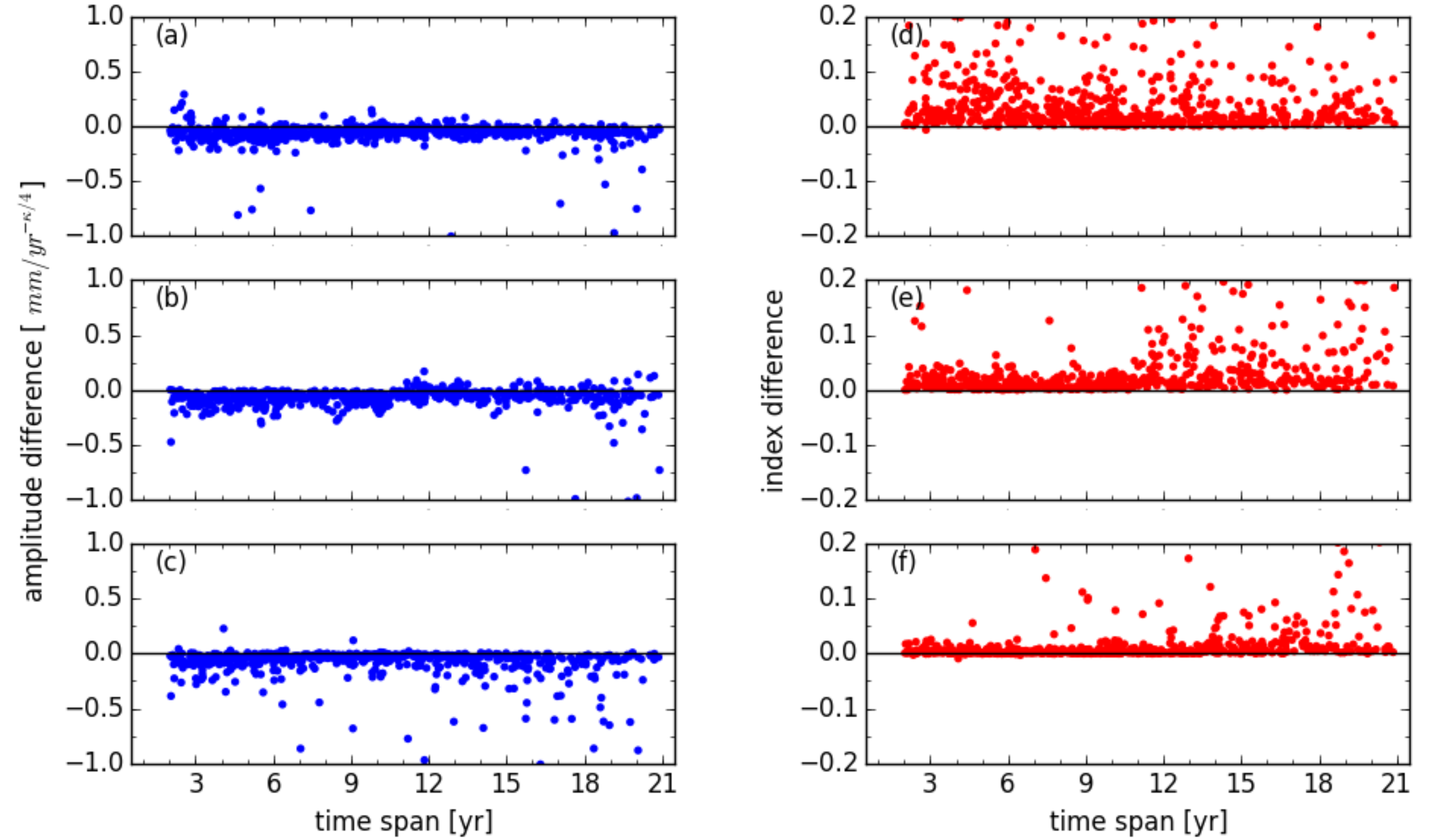
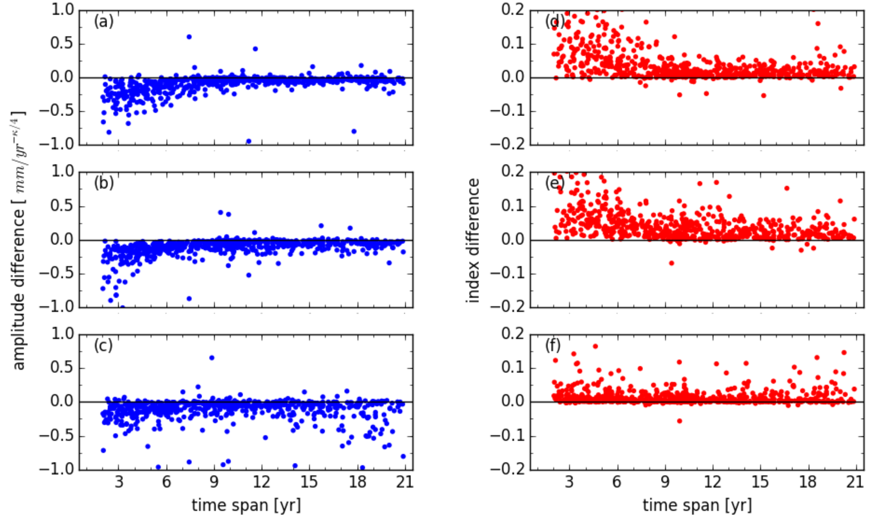
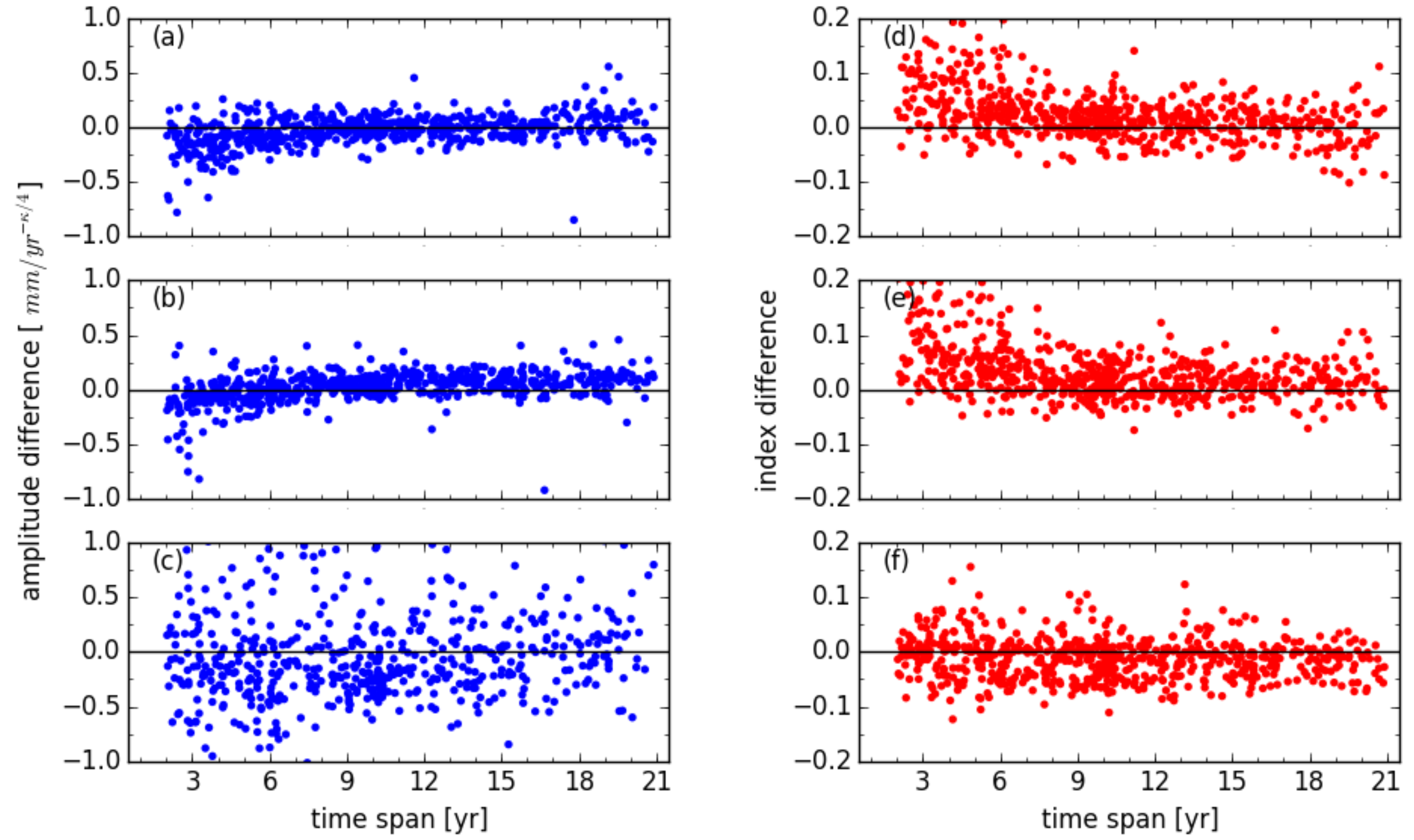
Figure 2 demonstrates the difference of power law noise between the estimation of simulated noise and the results from sim_unit_none.
There were 597 (91.2%), 597 (92.3%), and 632 (97.7%) of 647 stations with a smaller amplitude for sim_unit_none for the east, north, and up component, respectively. The median values of amplitude differences between the estimation of simulated noise and sim_unit_none were 0.05, 0.03 and 0.08 mm−k/4. There were also 73, 24, and 93 stations with amplitude differences larger than 0.2 mm−k/4 for the three components. With the increasing observation time span, the differences of amplitudes and spectral indexes are decreased and become stable.
Compared with the simulated noise, there were only 3 (0.5%), 8 (1.2%), and 6 (0.9%) stations with lower spectral indexes for sim_unit_none. For the spectral indexes, the median values of differences between estimated noise simulation and sim_unit_none were −0.02, −0.01, and −0.01 for east, north, and up components, respectively. There were also 59, 5, and 5 stations with spectral indexes differences larger than 0.1 for the three components. For the east component, more stations with a large spectral indexes difference may be related to the smaller amplitude of the annual signal. There were 164 stations with an observation time span of less than 6 years, and the median amplitudes of the annual signal were 0.6, 1.1, and 3.1 mm for the east, north, and up components, respectively. Compared with the amplitudes of north and up components, there were 75% and 92% stations with a smaller annual amplitude for east component, respectively. Considering the amplitudes of the simulated power law noise in the simulated observations, the results of the noise analyses of the east component seems to be more easily affected by seasonal signals, which needs further validation in the future.
Since no colored noise model was assumed in the generation of cumulative solutions, the systematic bias for the amplitudes and spectral indexes shown in
Figure 2 should be induced by the existence and estimation of seasonal signals in the deterministic model. Bosugz et al. also validated that the power law amplitudes decreased, and the spectral indexes were much “whiter” when all periodicities are subtracted from the position time series [
11].
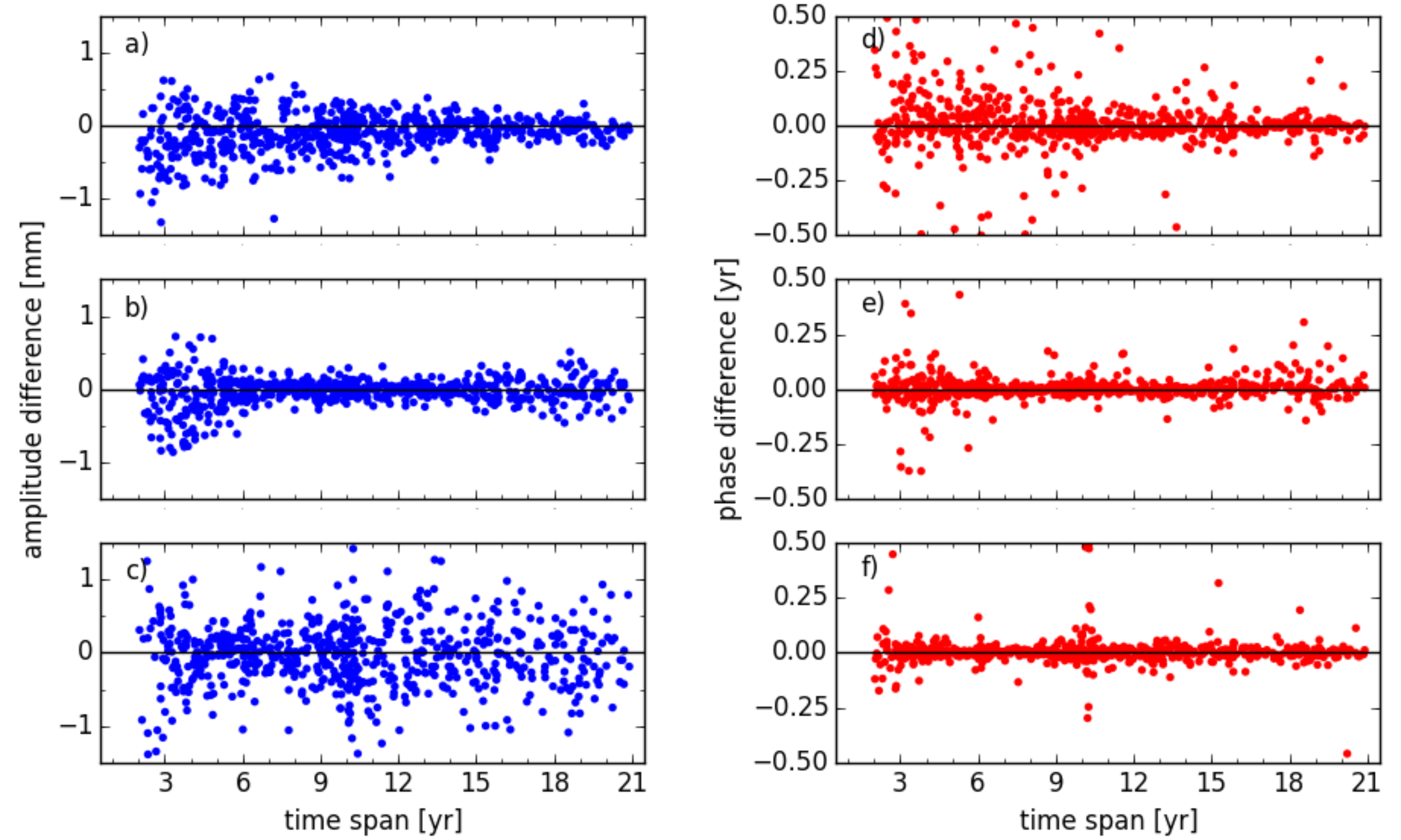
The differences of the annual amplitude and phase, between the raw simulated annual signal and estimation of solution sim_unit_none, are shown in
Figure 3. The amplitude difference of the up component was more scattered than the horizontal components, which is consistent with the larger amplitude difference of power law noise. The median values of the annual amplitude absolute difference were 0.15 ± 0.20, 0.09 ± 0.15, and 0.26 ± 0.37 mm for the east, north, and up components, respectively. Meanwhile, the median values for annual phase absolute difference were 11.52 ± 32.65, 5.40 ± 18.20, and 4.68 ± 18.80 degrees for the corresponding components. It is also noticed that the amplitude and phase differences of annual signal decreased with the increasing observation time span for the horizontal components.
3.2. Effect of the Weight Matrix on Noise Analyses
Both the simulated and real position time series were used to assess the effect of weight on the noise analyses of residuals.
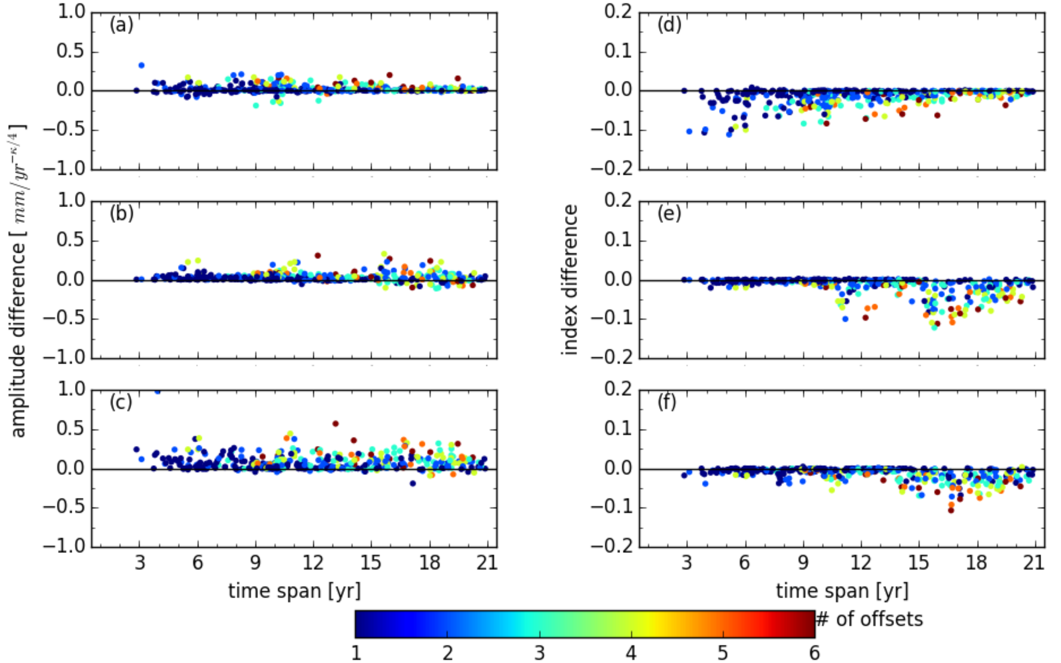
Figure 4 shows the comparison of the noise analyses between sim_unit_none and sim_cova_none. Since no offsets were simulated in the position time series and no Helmert transformation parameters modeled in the deterministic model, the differences of noise properties could be attributed to the weight matrix used for the observations. Compared to the solution without considering the spatial correlation (i.e., sim_unit_none), the noise of sim_cova_none with a full weight matrix seemed to more “colored”. There were 643 (99.4%), 646 (99.8%), and 630 (98.4%) stations for sim_cova_none with lower spectral indexes for east, north, and up components, respectively. The median values of the spectral indexes difference were 0.02, 0.01, and 0.01 for the three components. Moreover, there were 64, 57, and 35 stations with a spectral indexes difference larger than 0.1 for the east, north, and up components, respectively.
For the amplitude of the power law noise, there were 598 (92.4%), 602 (93%), and 616 (95.2%) stations for sim_cova_none with a larger amplitude than sim_unit_none for the east, north, and up components, respectively. The median values of amplitude difference were −0.05, −0.06, and −0.04 mm−k/4 for the three components. From the comparison of the noise analyses between sim_unit_none and sim_cova_none, it indicated that the spatial correlation derived from the covariance information could induce the shift toward flicker noise and enhance the amplitudes of colored noise.
Table 2 lists the statistical results of the annual amplitude and phase differences between the simulated annual signal and the estimation from different solutions. Compared with the simulated annual signal, both the amplitude and phase difference of the annual signal derived from sim_cova_none were more scattered than sim_unit_none. The absolute biases of the annual amplitude of sim_unit_none were 0.15, 0.09, and 0.26 mm for the east, north, and up components, respectively. While the median values of sim_cova_none were 1.5 times larger than the ones of sim_unit_none for each component. This indicates that both the noise characteristics and annual signal could be changed when the spatial correlation between different stations in the stacking solution was considered using the covariance information. Since the position time series of different stations could be affected by each other when the correlations were considered, the abnormal observations, such as the offsets and outliers in the position time series, should be checked carefully.
Using the practical IGS reprocessed daily solutions, the effect of different weight matrices could be assessed further.
Figure 5 shows the difference in power law noise between igs_unit_none and igs_cova_none. Considering the full weight matrix from the covariance information, a shift towards more “colored” noise was also found, which is similar to the simulation case. There were 621 (96%), 632 (97.7%), and 491 (91.3%) stations with lower spectral indexes for igs_cova_none for the east, north, and up components, respectively. The median values of the spectral indexes difference between igs_unit_none and igs_cova_none were 0.02, 0.03, and 0.01 for the three components.
It was also noticed that the spectral indexes difference decreased with the increasing observation time span, especially for the horizontal components, which was not similar to the results of simulation. For the stations with a time span of less than 8 years, the difference could even reach 0.2 or more. There were 74, 67, and 15 stations with spectral indexes difference larger than 0.1 for the east, north, and up components, respectively. For the amplitude of the power law noise, there were 605 (93.5%), 627 (96.9%), and 583 (90.1%) stations of igs_cova_none with larger amplitudes for the east, north, and up components, respectively. The median values of the amplitude difference were −0.05, −0.08, and −0.06 mm−k/4 for the three components.
3.3. Effect of Offset on Noise Analyses
In order to assess the effects of offsets in the position time series on noise characteristics, sim_unit_real was obtained by adding offset parameters in the functional model with the discontinuity information from the IGS for the 403 stations. It was clear that the additional offsets parameterized in the deterministic model could reduce the colored noise (
Figure 6), where the numbers of stations with spectral indexes closer to zero were 379 (94.0%), 378 (93.8%), and 382 (94.8%) for the east, north, and up components, respectively. Meanwhile, 295 (73.2%), 319 (79.2%), and 343 (85.1%) stations of sim_unit_real had a smaller amplitude of power law noise than sim_unit_none for the three components. It was also found that the more offsets in the position time series, the lower the spectral indexes difference that were obtained. However, this does not mean that more offsets were encouraged to be parameterized in the deterministic model to have much “whiter” noise. Instead of over-parameterization for the offsets in the position time series, it was much wiser to check the consistency of noise characteristics between the pieces before and after the offsets happening and decide whether to process the pieces together [
16,
17,
21].
Although the noise properties in the position time series could be changed by the intermittent offsets, the annual signal differences induced by the offsets were not significant. The median values of the annual amplitude absolute difference between sim_unit_none and sim_unit_real were 0.01 ± 0.03, 0.01 ± 0.02, and 0.03 ± 0.06 mm for the east, north, and up components, respectively. For the annual phase, the median values of the absolute difference between sim_unit_none and sim_unit_real were 0.72 ± 3.60, 0.72 ± 2.94, and 0.36 ± 2.76 degrees for the three components.
3.4. Effect of Helmert Transformation Parameters on Noise Analyses
The solutions with and without Helmert transformation parameters (three translation, three rotation, and one scale parameters) considered in the functional model were obtained and compared.
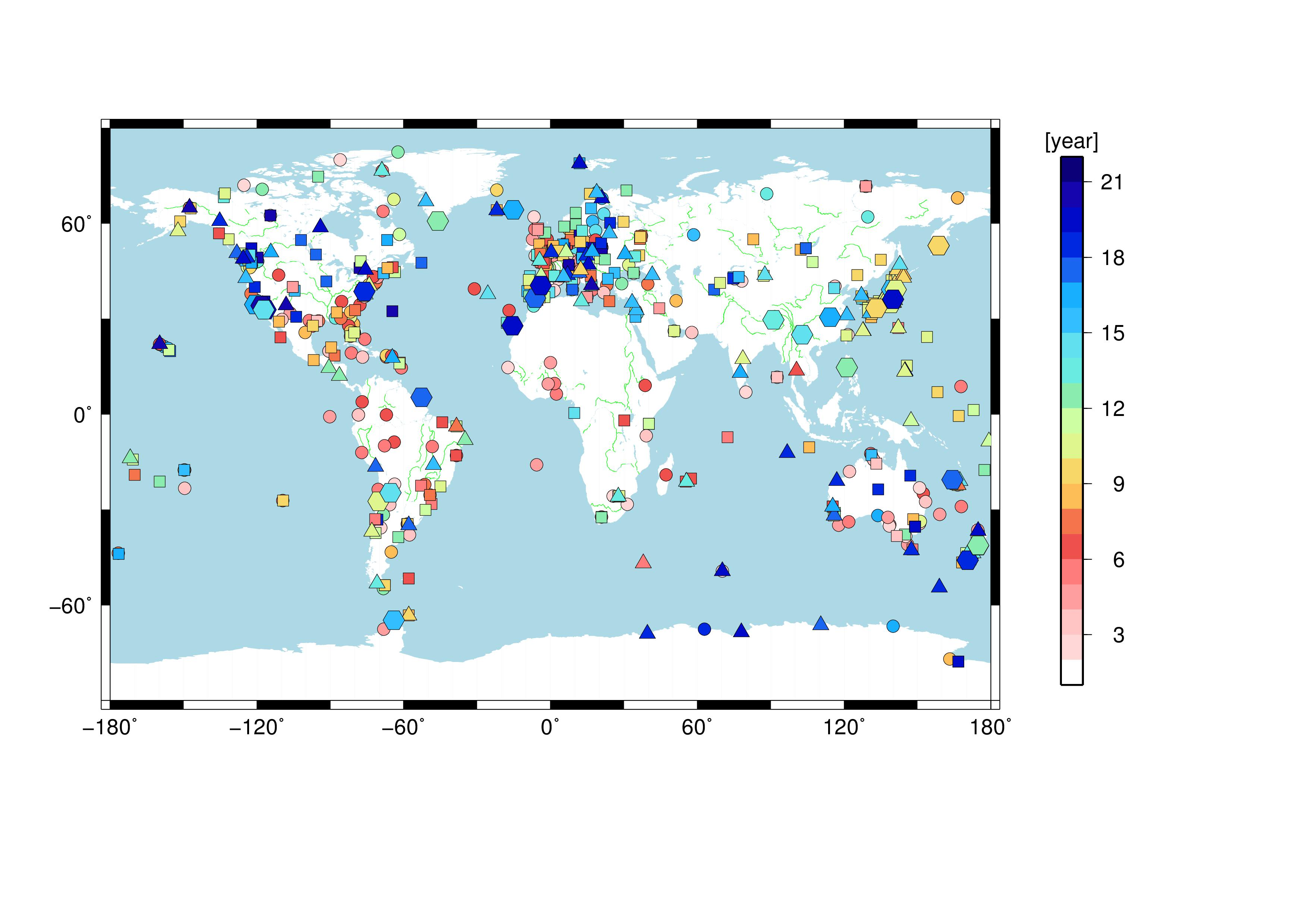
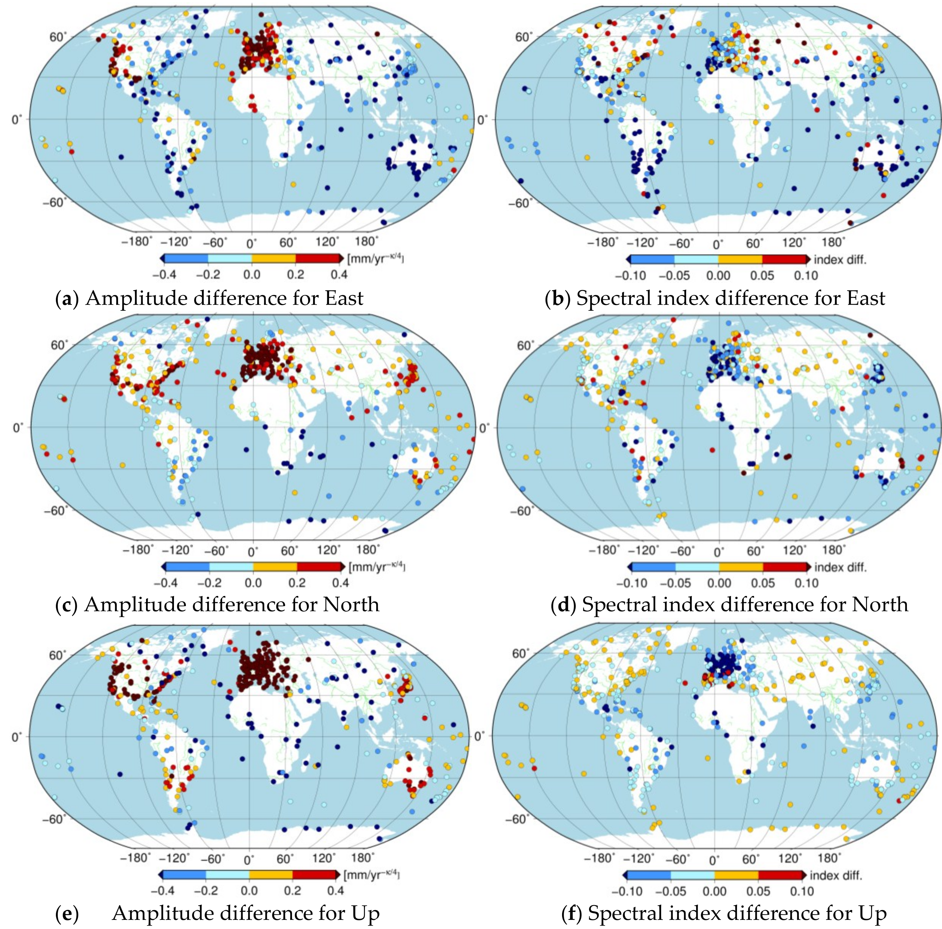
Figure 7 demonstrates the difference of power law noise between igs_unit_none and igs_unit_trs for the selected stations. For the spectral indexes, igs_unit_none had 474 (73.3%), 451 (69.7%), and 426 (65.8%) stations with lower spectral indexes for the east, north, and up component, respectively. A clear spatial dependence was noticed for the stations with more “colored” noise (i.e., lower spectral indexes) for igs_unit_trs, especially for the north and up components. For the north component, the inner continental stations in Asian areas for igs_unit_trs mostly have lower spectral indexes than igs_unit_none. For the up component, besides the stations in this inner continental region in Asia, the stations along the Antarctic and Baffin Bay coastline also showed lower spectral indexes for igs_unit_trs.
For the amplitude difference of power law noise between igs_unit_none and igs_unit_trs, there were 287 (45.4%), 458 (70.8%), and 431 (66.6%) stations with a larger amplitude for igs_unit_none for the east, north, and up components, respectively. Moreover, the stations with an amplitude difference larger than 0.4 mm
−k/4 were mainly situated within the Europe area. Collilieux et al. indicated that estimating the transformation parameters over the whole network could aliase the loading signals into the position time series [
40]. Here the authors validated that these additional parameters in the deterministic model could also induce systematic biases for the colored noise with different regional patterns and should be considered carefully [
19,
31].
3.5. Combined Effect of Helmert Transformation Parameters and Weight Matrix on Noise Analyses
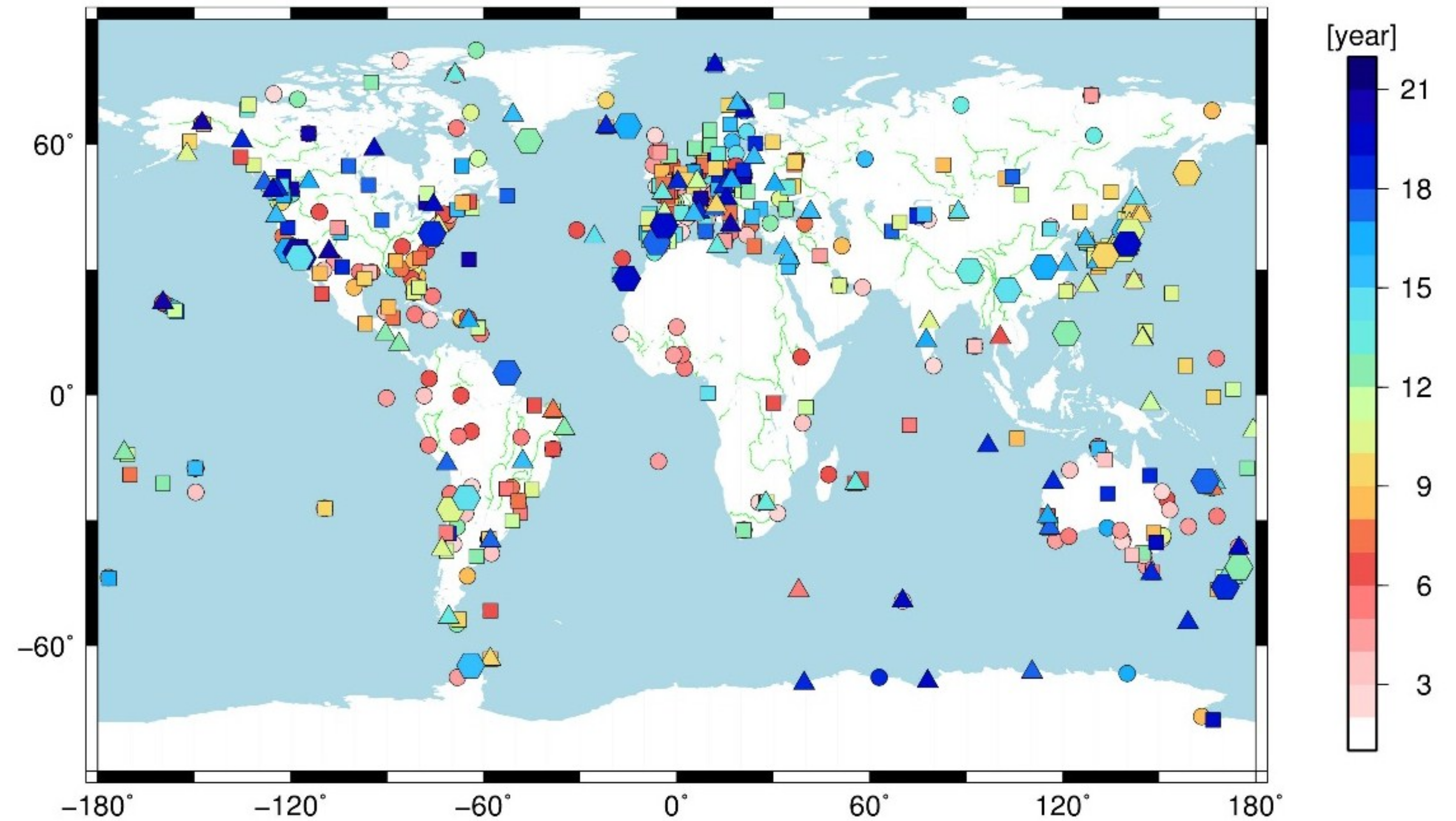
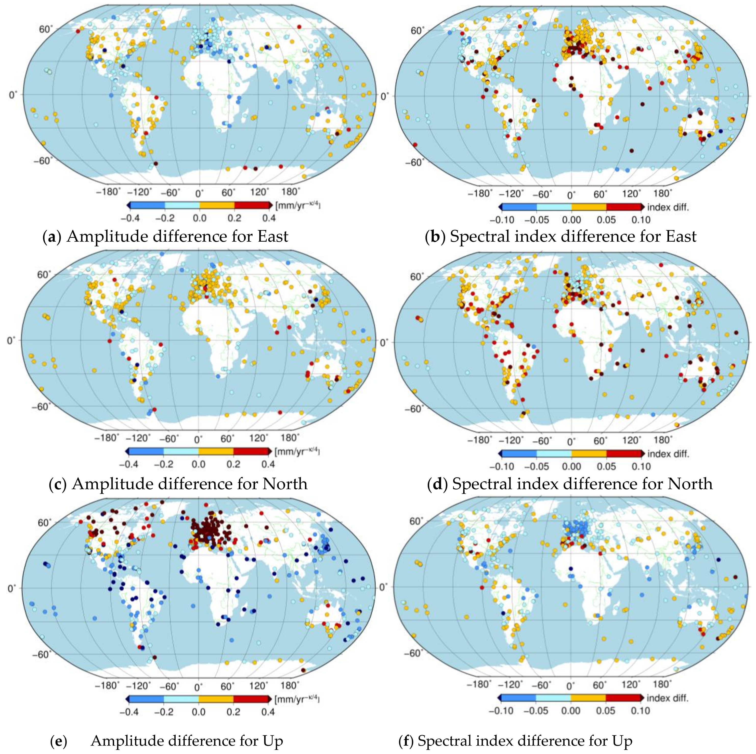
It was possible to assess the combined effect of Helmert transformation parameters and weight matrix on the noise analyses of the practical position time series through the comparison between igs_unit_none and igs_cova_trs. Considering the transformation parameters and full weight matrix derived from the covariance information, the noise of the solution igs_cova_trs showed different characteristics for the horizontal and up components. There were 471 (72.8%) and 499 (77.1%) stations for igs_cova_trs with lower spectral indexes for the east and north components, respectively. For the up component, there were only 249 (38.6%) stations with more “colored” noise (i.e., lower spectral indexes) for this solution. The stations with a different performance in the noise analyses for up component were mainly situated in the Europe area (
Figure 8). Klos et al. found a strong impact of the Baltic Sea on the position residuals of stations located in the Europe area and lower spectral indexes of the up component for stations in this area were obtained [
41]. Since the dense stations were located in the Europe area, this may result in colored noise that can be reduced significantly by the transformation parameters (especially the scale parameter) for the stations located in this area. The median values of spectral indexes between igs_unit_none and igs_cova_trs were 0.02, 0.02 and −0.01 for the east, north, and up components, respectively. Meanwhile, there were also 76, 63, and 117 stations with absolute spectral indexes larger than 0.1 for the three components.
For the amplitude difference of the power law noise, there was no systematic bias between igs_unit_none and igs_cova_trs, and there were 382 (59.0%), 235 (36.3%), and 337 (52.1%) stations for the solution igs_cova_trs with a larger amplitude for the east, north and up components, respectively. However, significant amplitude differences were found for stations located in the Europe area and near the equator. Moreover, there were 14, 15, and 249 stations with absolute amplitude differences larger than 0.4 mm−k/4 for the three components.
Figure 9 demonstrates the difference of the power law noise between igs_unit_none and igs_cova_trs over the observation time span. The spectral indexes differences for the stations with a time span of less than 8 years seemed to be more scattered than the other stations, especially for the horizontal components. A similar phenomenon was also noticed for the amplitude difference between igs_unit_none and igs_cova_trs.
Comparing the results of the noise analyses in
Section 3.2,
Section 3.4 and this section, it was found that the effects of the weight matrix and Helmert transformation parameters on the noise analyses showed different patterns. For most stations selected in this study, the weight matrix could enhance the colored noise, while the estimated transformaiton parameters were able to reduce the colored noise. When the two factors were considered together to obtain the stacking solution igs_cova_trs, a new pattern was again shown for the noise analyses, which could be contributed to the combined effects of the weight matrix and transformation parameters. For the horizontal components of the solution igs_cova_trs, the power law noises of global stations were mainly affected by the weight matrix, which had lower spectral indexes for most stations. However, the transformation parameters estimated in the functional model had more of an impact than the weight matrix on the power law noise for the up component. As a result, the transformation parameters, especially for the scale parameter, shifted the noise of the solution igs_unit_none toward much “whiter”.
4. Discussions
It is critical to have good knowledge about the noise characteristics in the GNSS position time series to obtain reliable velocity uncertainty, and assuming the only white noise in the position time series always overestimates the uncertainty of rate. Using the simulated and real GNSS position time series in this study, cumulative solutions with a least squares method and different strategies were obtained. The parameters of the power law noise plus white noise were then estimated for the residuals from different stacking strategies. The authors then assessed the effects of seasonal signals, the weight matrix used for observation, offsets in GNSS time series, and Helmert transformation parameters on the noise analyses of the residuals.
Table 3 summarizes the effects of variable factors on the noise of the residuals.
From the comparison of effects on noise analyses related to different variable factors (
Table 3), the largest impact on the power law noise was induced by the Helmert transformation parameters, which could reach 0.5 mm
−k/4 and 0.1 for the medians of amplitude and spectral index, respectively. For simplicity, a flicker noise with an amplitude of 1 mm
1/4 was assumed for the position time series with a 10-year time span, then the bias of the noise characteristics related to transformation parameters could cause an error of velocity of about 0.05 mm/yr, which should be taken into account for the increasing demand of high-precision velocity of 0.1 mm/yr [
42]. Moreover, the impact could be enlarged for stations with a shorter time span. For other factors, the effects on velocity uncertainty may be about 0.01 mm/yr when the noise estimation from the post residuals were used as a priori information. Further study is also needed to assess the effects on velocity estimations in detail but is out of the scope of this paper. Blewitt indicated that there is an equivalence between the deterministic model and stochastic model in the parameter adjustment, the unmodeled functional part could be shown in the stochastic and vice versa [
43]. Any inconsistencies between the deterministic and stochastic model can cause overestimation or underestimation for the parameters in both models. However, the accurate deterministic model was used for the simulated time series, but the power law noise of post residuals could still be biased from the a priori known noise information.
Fritsche et al. indicated that the contribution of GLONASS becomes considerable starting with the year 2008 for GNSS-related parameters (e.g., stations coordinates, Earth rotation pole parameters) [
44]. Distinct peaks were found at periods of 7.8 and 8.2 days in the position time series for analysis centers with GLONASS data processed in the second reprocess, which was close to the nominal ground period of the GLONASS satellite (8 days) [
29,
45]. When all significant periodic signals in position time series were considered, Bogusz and Klos indicated that the noise should be closer to white noise [
11]. Further comparison would be done for noise analysis of station position time series using GPS and GPS/GLONASS data.
5. Conclusions
Previous studies estimated the noise properties in the GNSS position time series and always took the annual and semi-annual signal into account in the functional model. However, they had seldom assessed the effect of the seasonal signal on the noise analyses. Compared with the simulated annual signal and noise, the mutual effects of seasonal signals and noise properties on each other were assessed in this study. Estimating the seasonal signals in the deterministic model resulted in much “whiter” noise for more than 98% of stations. For stations with an observation time span of less than 6 years, the spectral indexes difference could even reach 0.2. Meanwhile, the noise in the simulated position time series could also induce a median bias of 0.26 mm for the annual signal of the up component.
Using the current discontinuity information for GNSS position time series contributing to the ITRF2014, the effects of position/velocity offsets in simulated time series on the power law noise were assessed. The parameterization of the irregular offsets could induce spectral indexes closer to zero and smaller amplitudes for power law noise.
The effect of the weight matrix on noise analyses was assessed using the simulation as well as IGS second reprocessed solutions. The comparison indicated that the weight matrix derived from the covariance information could enhance the colored noise for more than 90% of stations. Moreover, using the simulated data, the median biases of the annual amplitude caused by different weight matrices could reach 0.2 and 0.4 mm for the horizontal and up components, respectively. When the additional Helmert transformation parameters were considered in the deterministic model, the colored noise of about 70% of stations were weakened for the three components, and a regional characteristic was also noticed for the spectral indexes difference. Finally, the transformation parameters and full weight matrix could result in 75% of stations with lower spectral indexes for the horizontal components. However, the percentage was only 40% for the up component, which indicated that weight matrix was the dominant factor for horizontal components while the transformation parameters were the dominant ones for vertical component. In order to obtain a velocity precision of 0.1 mm/yr for high-precision and long-term Earth science applications, the authors suggested that the Helmert transformation parameters should be considered carefully in the stacking model of position time series. Although the systematic bias could be caused by offsets and the weight matrix for the colored noise, the impacts of these systematic errors on velocity could be neglected.


