The Effects of Higher-Order Ionospheric Terms on GPS Tropospheric Delay and Gradient Estimates

Abstract

Atmospheric delays, e.g., ionospheric delay and tropospheric delay, are the dominant error sources for the Global Navigation Satellite System (GNSS), especially for Precise Point Positioning (PPP). The common method for eliminating ionospheric delay is to form an ionosphere-free (IF) observable, which is a linear combination of observables on two frequencies such as GPS L1 and L2. As for the tropospheric delay, the dry component can be precisely corrected by empirical models, while the wet component is usually estimated as unknowns. However, the higher-order ionospheric (HOI) terms are not totally cancelled out in the (first-order) IF observable and as such, when not accounted for, they degrade the accuracy of other parameters. The impact of HOI corrections is well documented in the literature. This paper investigates the temporal effects of HOI terms on estimated tropospheric parameters, i.e., zenith tropospheric wet delay (ZWD) and north and east gradients. For this purpose, observations from over 100 stations with good global coverage were used considering various geographic and geophysical conditions. The results of numerical experiments show that HOI effects have a significant impact on the estimated tropospheric parameters, and the influence is dependent on location and time. The maximum differences of ZWD estimates reach over 20 mm during periods of activity such as solar storms and geomagnetic storms. Additionally, the north gradients are more likely to be affected by HOI effects compared with east gradients. In particular, the tropospheric gradient component is most affected for low latitude station during daytime. Additionally, the effects of bending errors and HOI terms on slant tropospheric delay at low elevation angles are much larger than those at high elevation angles.

1. Introduction

Global Navigation Satellite System (GNSS) signals are delayed and refracted by the neutral atmosphere and ionosphere individually when propagating through the atmosphere, phenomena that are usually referred to as the “tropospheric delay” and “ionospheric delay.” The former is one of the major error sources in GPS positioning, which contributes a bias of several decimeters in humid regions in the vertical direction even when recorded meteorological data are simultaneously exploited in tropospheric models [1,2]. Based on physical properties, the zenith tropospheric delay (ZTD) can be divided into zenith hydrostatic delay (ZHD) and zenith wet delay (ZWD) components. ZHD is aroused by the dry gas content in the troposphere, which can be precisely determined from meteorological data using empirical models [3,4], while ZWD is caused by water vapor in the troposphere and is difficult to model accurately. The ionospheric delay, which arises from the interaction between the ionosphere and the geomagnetic field, also accounts for inferior GNSS positioning [5]. Due to the dispersive nature of the ionosphere, the first-order ionospheric delay can be mitigated by forming an ionosphere-free (IF) observable on two frequencies [6]. The IF observable can eliminate about 99.9% of the total ionospheric effect yielding an accuracy sufficient for most GNSS applications [7]. For GNSS applications which demand high accuracy, such as precise point positioning (PPP) and real time kinematic positioning (RTK), especially during the peaks of the solar cycle, higher-order ionospheric (HOI) terms, i.e., the second- and third-order delays, need to be considered, as they can cause range errors of a few centimeters to tens of centimeters [8].

HOI delays and their effects on GNSS positioning have been investigated in numerous studies. Brunner and Gu [9] developed correction models based on geomagnetic field and ionospheric parameters for HOI terms, especially to correct the second order term and ray-path bending errors. Bassiri and Hajj [10] proposed simplifications to the modelling, such that the terms could be modelled practically, and limited their consideration to second- and third-order effects, with no bending effects. Although HOI terms are much less than 1% the strength of the first-order term at GPS frequencies, they may deteriorate the estimation accuracy of geodetic parameters. Petrie et al. [11] showed that ignoring HOI delays results in spurious southward shifts in GPS-derived origin of the terrestrial reference frame along the Earth’s spin axis. In terms of PPP, studies have shown that when satellite orbits and clocks are held fixed, the HOI delay leads to a northward shift of stations [12,13]. With HOI delay accounted for, the estimated station coordinates in PPP can differ at the millimeter to centimeter level, and the convergence time can be shortened by about 15% [7,14,15]. Deng et al. [16] investigated the effects of HOI delay on GPS coordinate time series in regional networks and found that HOI corrections can effectively reduce the semi-annual signals in the northern and vertical components. Recently, increasing attention has been paid to the effects of HOI delay on satellite-related products, i.e., orbits and clocks, which captured most of the impact of HOI corrections, with a magnitude of up to 2 cm for clock corrections, 1 cm for the along-track and cross-track components, and below 5 mm for the radial component [17,18].

As a by-product of PPP, the tropospheric delay will also be affected by the HOI terms. However, little attention has been paid to the impact of HOI effects on the estimated tropospheric parameters. Zus et al. [19] investigated the impacts of HOI terms on estimated tropospheric parameters by comparing the tropospheric estimations of different ionospheric processing strategies (ionospheric corrections applied or not applied). Additionally, investigation has shown that HOI corrections must be applied in the field of high-precision GPS geodesy. Even though several authors have considered the effects of HOI terms on tropospheric parameters, previous works have mainly focused on the effects of HOI terms on monthly or seasonal averages in high or medium solar activity. There are relatively few studies devoted to revealing the temporal effects of HOI terms. However, the temporal errors of tropospheric estimated parameters caused by HOI terms are more valuable to GPS real-time meteorological studies.

Tropospheric parameters, while considered as nuisance parameters in geodesy, are in fact regarded as a useful data source for meteorological studies [20]. Therefore, we aim to investigate the impacts of HOI effects on tropospheric parameters in this paper. Both the ZWD and gradient estimates are analyzed with different ionospheric activity characteristics.

The structure of this paper is as follows. After the introduction in Section 1, the datasets and processing strategies for HOI correction and tropospheric delay estimation are described in Section 2. The results and analyses are presented in Section 3. Finally, the conclusions are given in Section 4.

2. Materials and Methods

2.1. Datasets and Processing Strategies

The observational data used in our study were collected from over 100 GPS stations of the International GNSS Service (IGS) Network (Figure 1), aiming for a reasonably latitudinal and longitudinal coverage around the world. These evenly distributed stations are located in different environments including prairie, forest, desert, island and coastline, and can thus represent diverse climatic conditions.

Datasets from day of year (DOY) 237 to 257 in 2017 were processed to investigate the impact of HOI effects on tropospheric estimation under different ionospheric conditions. As shown in Figure 2, a strong solar storm occurred on DOY 248 in 2017, as confirmed by the solar index F10.7 obtained from the GODDARD space flight center (https://omniweb.gsfc.nasa.gov/form/dx1.html). Subsequently, a geomagnetic storm affected by the strong solar storm was detected in the following 2–3 days. It started at about 3:00 UT on DOY 250 in 2017 and reached a maximum Kp value of 8 at about 1:00 UT on DOY 251 in 2017, accompanied by a Dst value as low as –142 nT and one peak AE value of 2677 nT. The geomagnetic index series can be obtained from the World Data Center in Kyoto (http://wdc.kugi.kyoto-u.ac.jp/wdc/Sec3.html). Herein, we define the period in which solar storms or ionospheric storms occurred as “active period” (DOY 247–252 in 2017) and the period with low geomagnetic index and solar index as “quiet period” (DOY 237–243 in 2017).

Table 1. Processing strategies of precise point positioning (PPP) for tropospheric parameters retrieval.

Item	Processing Strategies
Observation	Ionosphere-free (IF) combination
Signal selection	L1 and L2
Sampling rate	30 s
Elevation mask	10°
Weight for observations	Elevation-dependent weighting scheme
Estimator	Kalman filter
Ionosphere	with and without HOI corrections [21]
Tropospheric mapping function	GMF [2]
Satellite orbit	IGS final precise ephemeris products
Satellite clock	IGS final precise clock products
Coordinates of stations	Fixed with SINEX product
Phase center offset and variation	IGS Convention [22]
Phase windup effect	Corrected [23]
Receiver clock	Estimated as white noise
Tropospheric wet delay	Estimated as random-walk model. RWPN*: $5\times {10}^{-4}{\mathrm{m}\mathrm{s}}^{-1/2}$
Tropospheric gradients	Estimated as random-walk model. RWPN: $5\times {10}^{-5}{\mathrm{m}\mathrm{s}}^{-1/2}$

* RWPN: random walk process noise.

summarizes the detailed processing strategies of PPP. GPS L1 and L2 observations with 30-s samples were used to form IF combinations. The satellite elevation mask was set at 10°, and the elevation-dependent weighting scheme was adopted in a Kalman filter:

$$\sigma =a^2/{\sin }^{2}E$$

(1)

where $\sigma$ denotes the variance of observation, a is a constant which is generally set to be 0.003 m for carrier phase and 0.3 m for code observations, and $E$ is the elevation angle (unit: rad).

Since the coordinates of IGS stations are precisely known, they were held fixed in the Kalman filter. The IGS final precise ephemeris and clock products with an accuracy of 2–3 cm were used to mitigate the satellite orbits and clock errors. Satellite and receiver phase center offsets and variations, as well as phase wind-up effect, were precisely corrected by empirical models. Global Mapping Function (GMF) was employed for the estimation of tropospheric delay [2]. The zenith tropospheric wet delay (ZWD) and gradients were estimated as a random-walk model, while the receiver clock bias was estimated as white noise. The program RINEX_HO was employed to correct GPS observables for HOI terms. In this program, the geomagnetic field is computed by the IGRG12 model, and the total electron content (TEC) can be interpolated from global ionospheric maps (GIM). For more details please refer to reference [21].

2.2. Methodology

When a GPS signal propagates through the ionosphere, phase advance and code delay occur, and the raypath bends [24,25,26]. Only the phase advance caused by HOI terms will be considered in our study, because the effects of HOI terms in pseudorange measurements are distorted by noise and multipath error.

2.2.1. Ionospheric Delay Expression

The refractive index n for a radio wave at a given frequency $f$ is approximately given by reference [9]:

$$n=1+K_1\frac{Ne}{f^2}-K_2\frac{Ne}{f^3}-K_3\frac{Ne}{f^4}$$

(2)

where $Ne$ stands for the electron density, $K_j$ (j = 1,2,3), which can be written as:

$$\{\begin{array}{l}{K}_1=\frac{e^2}{8{\pi }^2\cdot {\epsilon }_0\cdot m}\\ K_2=\frac{{\mu }_0\cdot e^3\cdot B_0\cdot \cos \theta }{16{\pi }^3\cdot {\epsilon }_0\cdot m^2}\\ K_3=\frac{e^2}{128{\pi }^4{\epsilon }_0^3{m}^2}\end{array}$$

(3)

where $e\approx 1.6022\times {10}^{-19}$ is the electron charge, ${\epsilon }_0=8.854187817\times {10}^{-12}\mathrm{F}/\mathrm{m}$ is the free space permittivity, ${\mu }_0=12.57\times {10}^{-7}\mathrm{H}/\mathrm{m}$ denotes the permeability in the vacuum, $m\approx 9.10939\times {10}^{-31}\mathrm{kg}$ denotes the electron mass, $B_0$ is the magnitude of the geomagnetic induction vector $B$, and $\theta$ is the angle between the geomagnetic field vector and the radio wave propagation direction.

The propagation of a GPS signal through the ionosphere follows Fermat’s principle, and the signal path length can be recognized as the line integral along the raypath $l$ [27]:

$$L={\displaystyle \underset{l}{\int }nds}$$

(4)

The raypath bending error $\Delta s_{b(\mathrm{length})}$ is defined as the residual error due to excess path length, which is subtractive in the ionospheric phase advance:

$$\Delta s_{b(\mathrm{length})}={\displaystyle \underset{l}{\int }ds}-\rho$$

(5)

where $\rho$ denotes the geometric distance between the satellite and receiver:

$$\rho =L+{\displaystyle \underset{l}{\int }(1-n)ds}-\Delta s_{b(\mathrm{length})}$$

(6)

where ${\displaystyle \underset{l}{\int }(1-n)ds}$ refers to the ionospheric phase delay of frequency $f_j$, denoted as $I_j$:

$$I_j={\displaystyle \underset{l}{\int }(1-n)ds}$$

(7)

Compared with the phase delay error, the ray path bending error is smaller by about three orders of magnitude, however at low elevation angles the bending effects can be more significant than the third-order effect [27,28].

Assuming a right-hand circularly polarized signal, the ionospheric delay error can be formulated as:

$$I_j=\frac{p}{f^2}+\frac{q}{f^3}+\frac{t}{f^4}$$

(8)

in which,

$$\{\begin{array}{l}p=\frac{e^2}{8{\pi }^2\cdot {\epsilon }_0\cdot m}{\displaystyle \underset{l}{\int }Neds}\\ q=-\frac{{\mu }_0\cdot e^3\cdot B_0\cdot \cos \theta }{16{\pi }^3\cdot {\epsilon }_0\cdot m^2}{\displaystyle \underset{l}{\int }Neds}\\ t=-\frac{e^2}{128{\pi }^4{\epsilon }_0^3{m}^2}{\displaystyle \underset{l}{\int }Neds}\end{array}$$

(9)

where $\frac{p}{f^2}$ is the first-order ionospheric term and $\frac{q}{f^3}$ and $\frac{t}{f^4}$ denote the second- and third-order ionospheric terms, respectively, which are commonly defined as HOI terms, $B_0$ and $\theta$ will be estimated at the ionospheric pierce point (IPP) [10,21].

2.2.2. GPS Observation Equation

For GPS, the carrier phase ${\Phi }_j$ and code pseudorange $P_j$ of a specific frequency $j$ can be expressed as:

$$\{\begin{array}{l}{\Phi }_j=\rho +c\cdot (t_r-t^s)+N_j\cdot {\lambda }_j+B_j+T_{rop}+{\epsilon }_j-I_j\\ P_j=\rho +c\cdot (t_r-t^s)+b_j+T_{rop}+I_j+e_j\end{array}$$

(10)

where $t_r$ and $t^s$ denote the receiver clock bias and satellite clock bias, respectively, c is the speed of light in a vacuum, $N_j$ is the integer ambiguity of carrier phase, $B_j$ stands for the uncalibrated phase delays (UPD), ${\lambda }_j$ is the wavelength of carrier phase, $b_j$ denotes the code biases caused by hardware delays, $T_{rop}$ denotes the slant tropospheric delay and ${\epsilon }_j$ and $e_j$ are the sum of remained errors, such as multipath error and observation noise, for the carrier phase and pseudorange observation, respectively.

Traditionally, the IF combinations shown in Equation (9) are widely used to eliminate the first-order ionospheric delay, leaving the HOI terms uncorrected.

$$\{\begin{array}{l}{\Phi }_{IF}=\frac{1}{f_1^2-f_2^2}(f_1^2{\Phi }_1-f_2^2{\Phi }_2)=\rho +c\cdot dt+T_{rop}+B_{IF}+N_{IF}+{\epsilon }_{IF}+HOI\\ P_{IF}=\frac{1}{f_1^2-f_2^2}(f_1^2{P}_1-f_2^2{P}_2)=\rho +c\cdot dt+T_{rop}+b_{IF}+e_{IF}\end{array}$$

(11)

$$\{\begin{array}{l}{N}_{IF}=\frac{1}{f_1^2-f_2^2}(f_1^2{\lambda }_1{N}_1-f_2^2{\lambda }_2{N}_2)\\ B_{IF}=\frac{1}{f_1^2-f_2^2}(f_1^2{B}_1-f_2^2{B}_2)\\ HOI=\frac{q}{f_1^2{f}_2+f_2^2{f}_1}+\frac{t}{f_1^2{f}_2^2}\\ b_{IF}=\frac{1}{f_1^2-f_2^2}(f_1^2{b}_1-f_2^2{b}_2)\\ dt=(t_r-t^s)\end{array}$$

(12)

where $N_{IF}$ is the ambiguity of the IF combination and is no longer integer, $B_{IF}$ and $b_{IF}$ refer to the uncalibrated phase delay and code delay of IF combination, respectively, and ${\epsilon }_{IF}$ and $e_{IF}$ denote the sum of multipath error and noise for the IF observation. HOI is the combined effect of the higher-order ionospheric delays. $dt$ is the clock difference between receiver and satellite.

2.2.3. HOI Correction and Tropospheric Delay Estimation

An HOI term can be described as a function of the TEC and geomagnetic induction [10,29,30]. In general, the geomagnetic induction can be calculated from a geomagnetic reference system by using a dipolar model with an accuracy of approximately 75%, and the approximation obtained from the more realistic geomagnetic field has a higher accuracy, within millimeter level [21]. In this study, the International Geomagnetic Reference Field (IGRF 12) was employed to obtain the geomagnetic induction. To compute the TEC from pseudoranges, differential code bias (DCB) data were obtained from the center for orbit determination in Europe (CODE).

$${\displaystyle \int Neds}=TEC$$

(13)

$$\{\begin{array}{l}HOI=\frac{q}{f_1^2{f}_2+f_2^2{f}_1}+\frac{t}{f_1^2{f}_2^2}\\ q=-\frac{{\mu }_0\cdot e^3\cdot B_0\cdot \cos \theta \cdot TEC}{16{\pi }^3\cdot {\epsilon }_0\cdot m^2}\\ t=-\frac{e^2\cdot TEC}{128{\pi }^4{\epsilon }_0^3{m}^2}\end{array}$$

(14)

The precise point positioning (PPP) method was used extensively for tropospheric delay retrieval in this study. For more information about PPP implementation, refer to references [31,32]. The tropospheric delay consists of hydrostatic and wet components, and can be obtained through a mapping function related to the elevation angle $e$ and azimuth angle $a$:

$$T_{rop}(e,a)=m_h(e)\cdot Z_h+m_w(e)\cdot Z_w+m_g(e)\cdot [\cos (a)\cdot G_n+\sin (a)\cdot G_e]$$

(15)

where $m_h$, $m_w$ and $m_g$ denote the hydrostatic, wet and gradient mapping functions, respectively, $Z_h$ and $Z_w$ refer to ZHD and ZWD, and Gn and Ge denote the north gradient and east gradient, respectively. The ZHD can be precisely calculated using meteorological model [2,3], while the ZWD and the two gradient components $G_n$ and $G_e$ are usually estimated as unknowns. Thus, the parameters vector X for PPP can be expressed as follows:

$$X=(t_r,Z_w,G_n,G_e,{\overline{N}}_{IF})$$

(16)

$${\overline{N}}_{IF}=N_{IF}+B_{IF}$$

(17)

where $t_r$ is the receiver clock bias and ${\overline{N}}_{IF}$ is the estimable carrier phase ambiguity coupled with integer ambiguity and uncalibrated phase delays. Since the station coordinates are held fixed, the HOI terms will only be absorbed by the tropospheric parameters, ambiguities and clocks.

3. Results and Discussion

Considering that an HOI term is a function of TEC and geomagnetic field, three experiments were designed to investigate the relationship between HOI terms and tropospheric parameter estimation in different situations. The first two experiments showed the impact of HOI effects on ZWD estimation in different TEC and geomagnetic conditions, using both daytime and night-time data, as well as data collected from active and quiet ionospheric periods. The last one reflected the way the HOI terms affect tropospheric horizontal gradient estimation and slant tropospheric delay retrieval with different ray location in 3D space.

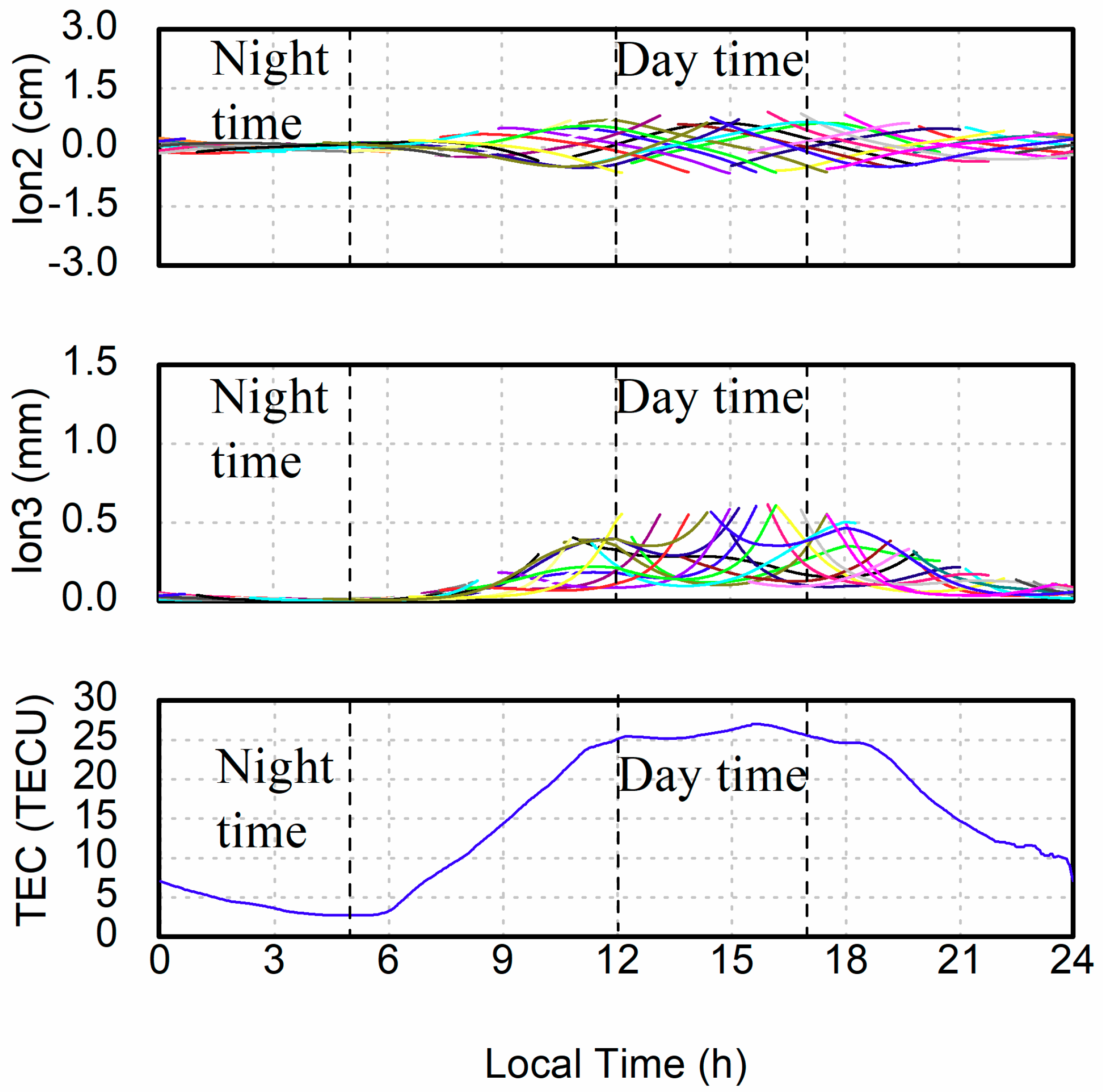
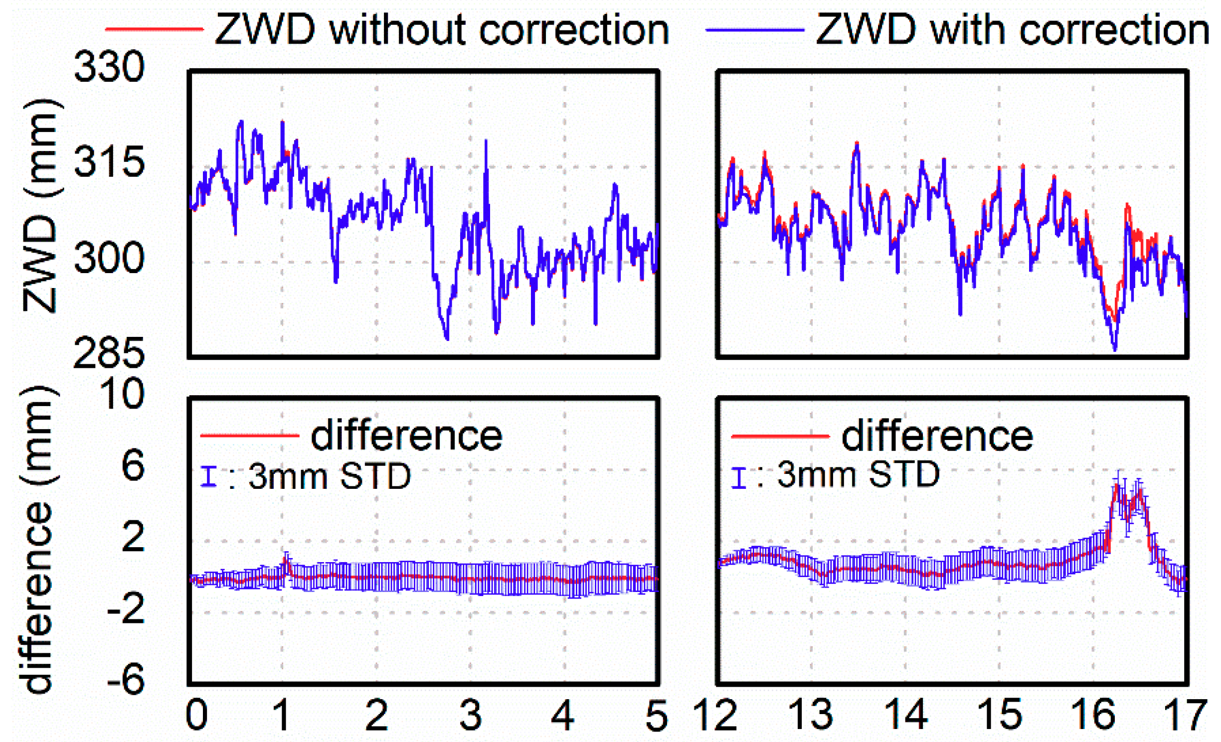
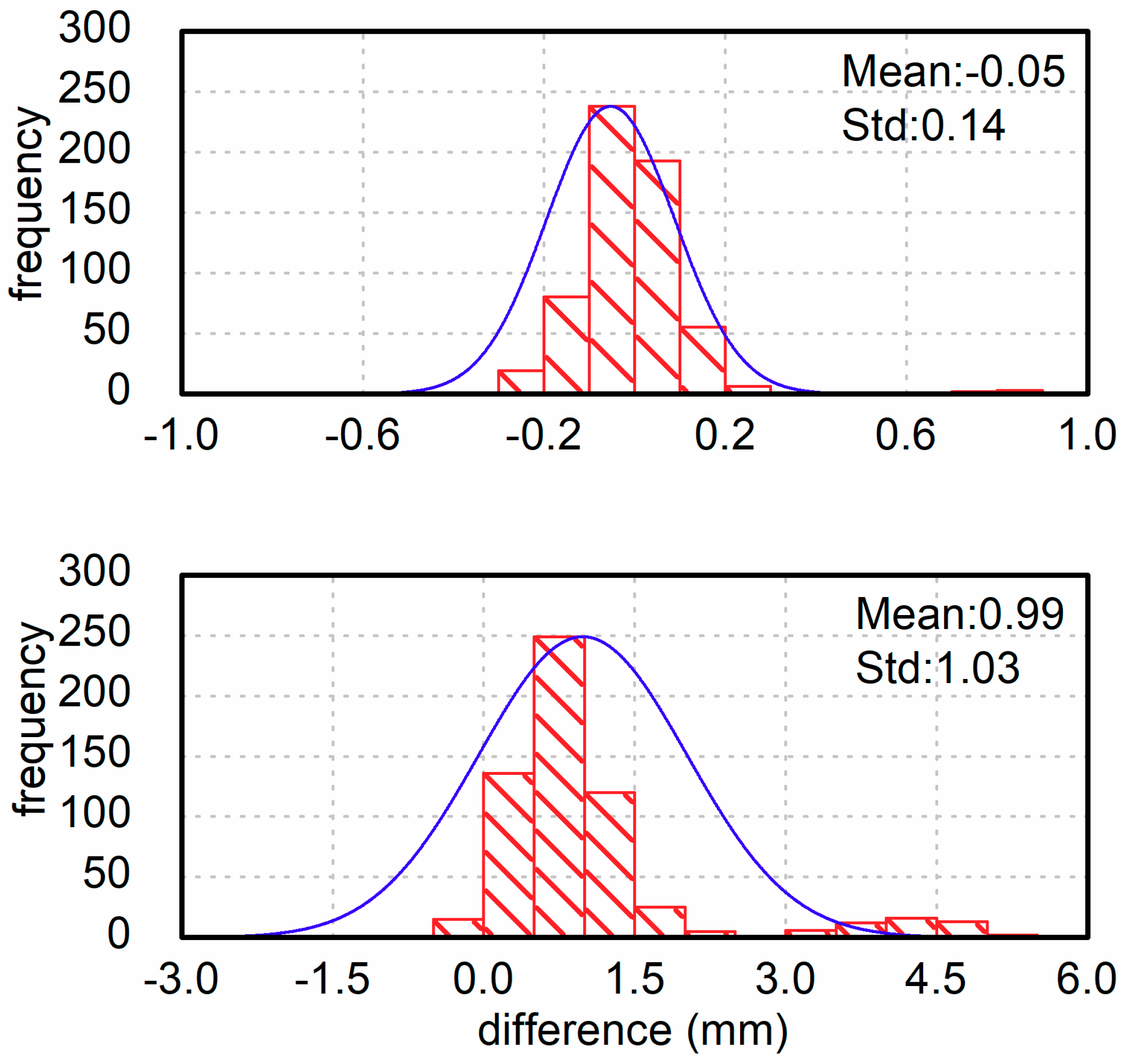
3.1. HOI Effects in Different TEC Conditions

The second- and third-order ionospheric delay (i.e., Ion2 and Ion3) and the vertical TEC (vTEC) value of station YKRO observed on DOY 239 are shown in Figure 3. The period of 0–5 LT was selected to represent night-time, and the period of 12–17 LT was selected to represent daytime. vTEC values can be seen to vary from a few TECU at night-time to tens of TECU in the daytime. Since the effects of vTEC variations are much larger than those of changes in geomagnetic induction, the HOI delays during the daytime are clearly larger than those at night.

Figure 4 shows the ZWD estimates with and without HOI corrections. The differences of the ZWD estimates and the error bars are also shown in Figure 4. During the night-time, the ZWDs agree well with each other, and the differences are mostly smaller than 1 mm, meaning that the impacts of the HOI effect on ZWD are marginal. However, as expected, the influences of the HOI effect on ZWD estimation are more profound during the day. The ZWD estimates can differ by up to 5 mm, particularly during the period of 16–17 LT, when the vTEC reaches approximately 25 TECU.

The distributions of ZWD differences are presented in Figure 5. The ZWD differences are almost normally distributed at night, while the distribution of ZWD differences is significantly tailed in the daytime. The mean values and standard deviations of ZWD differences are also shown in Figure 5 for comparison. The mean difference of HOI effect on ZWD estimation is –0.05 mm with a standard deviation of 0.14 mm at night, while the mean difference reaches 0.99 mm with a standard deviation of 1.03 mm in the daytime.

ZWD differences may be even greater when the vTEC values are larger during active periods. To verify this, we analyzed the relationship between the influences of HOI terms and vTEC values. Figure 6 shows the HOI terms of GPS L1 for station COCO in the active and quiet period. The values of HOI terms during the active period are clearly significantly larger than those during the quiet period. The vTEC values during the active and quiet period are presented in Figure 7. For both active and quiet periods, the night-time vTEC values are nearly identical, with a few TECU. However, the situation is different in the day-time, when the value of vTEC reaches a maximum of 35 TECU at noon for the active period, and is within 15 TECU for the quiet period.

The ZWD estimates with and without HOI corrections and their differences for COCO during the quiet and active period are shown in Figure 8. At night, the ZWD estimates with and without HOI corrections agree well, within 0.1 mm for both periods. However, the ZWD estimates differ by a maximum of 4 mm and 12.9 mm in the day-time for the quiet and active periods, respectively. The differences may be even larger for stations located at low latitude in special circumstances, such as during solar storms and geomagnetic storms. For example, at station MKEA the ZWD differences reach a maximum of 21.3 mm on DOY 248 in 2017, which must be corrected for precise atmospheric applications. Due to space limitation, the results are not shown in this paper.

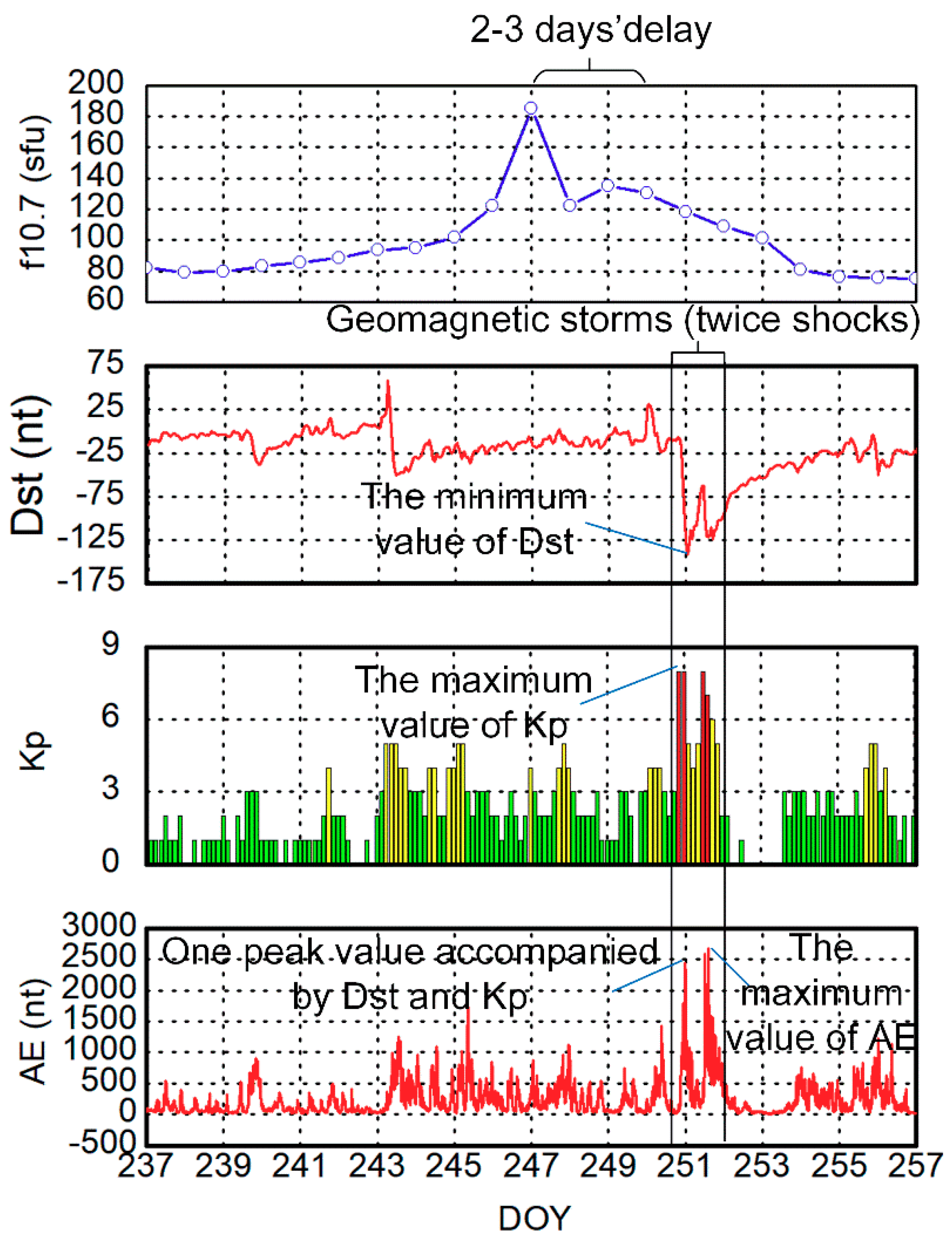
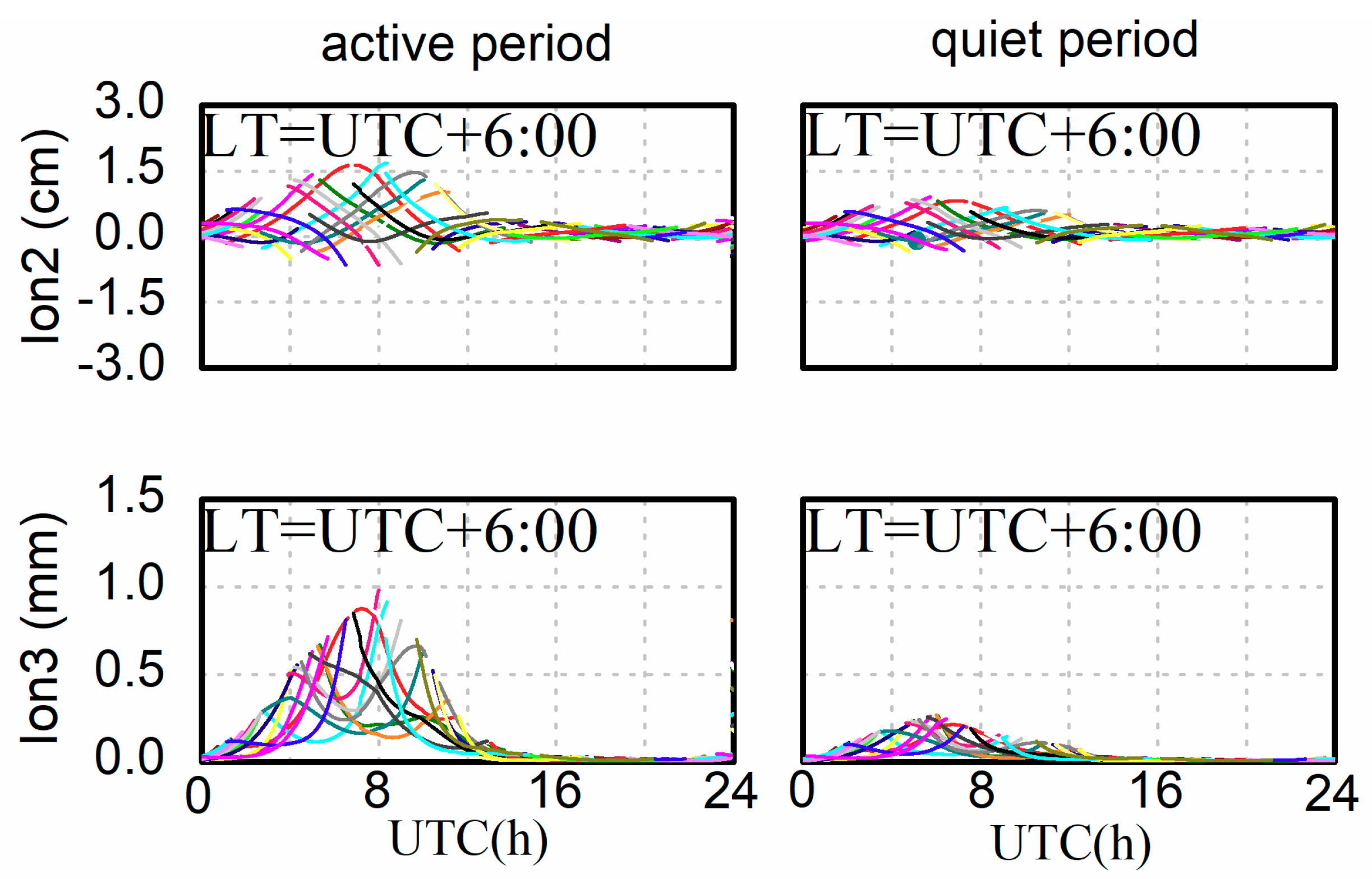
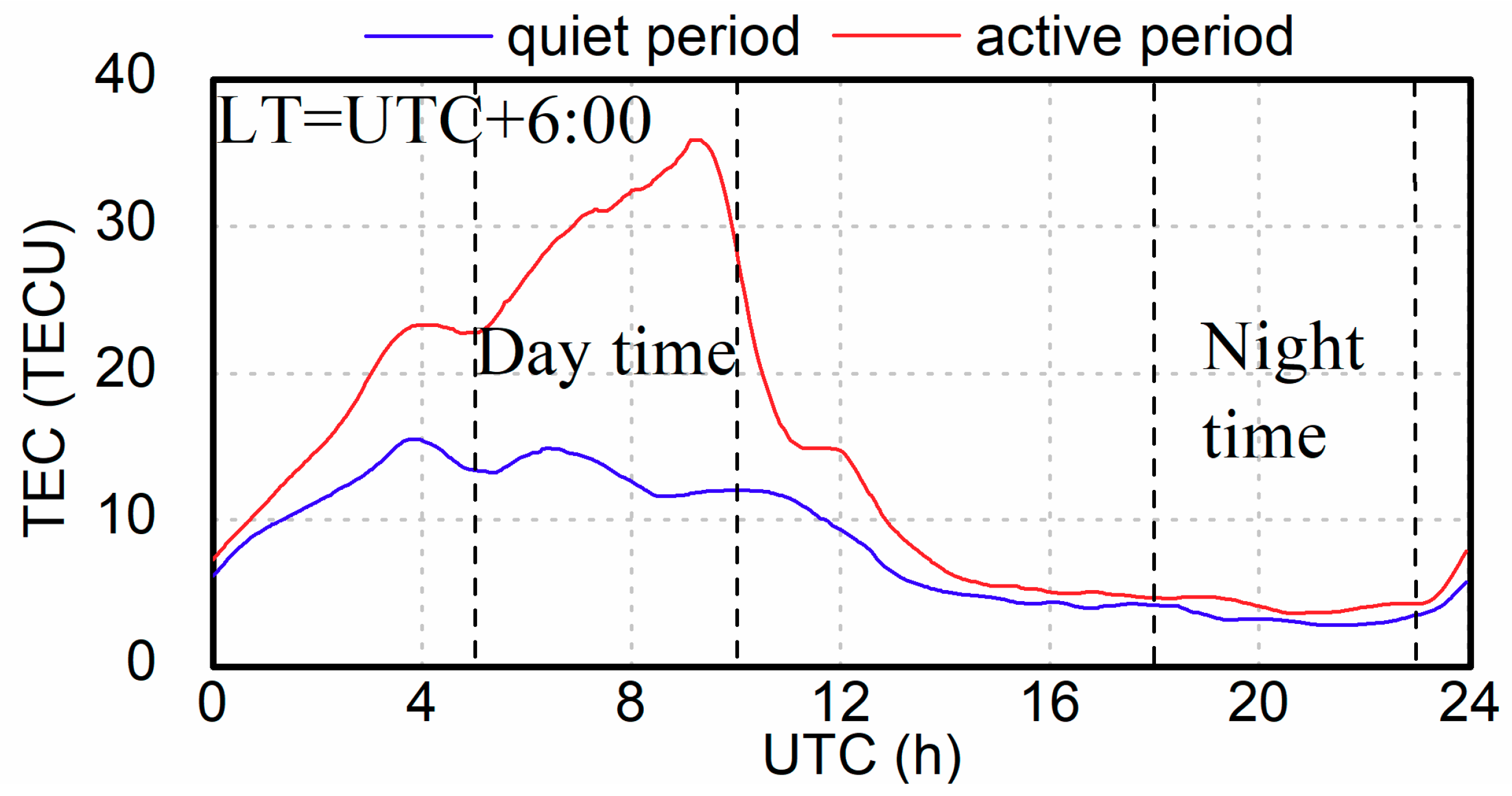
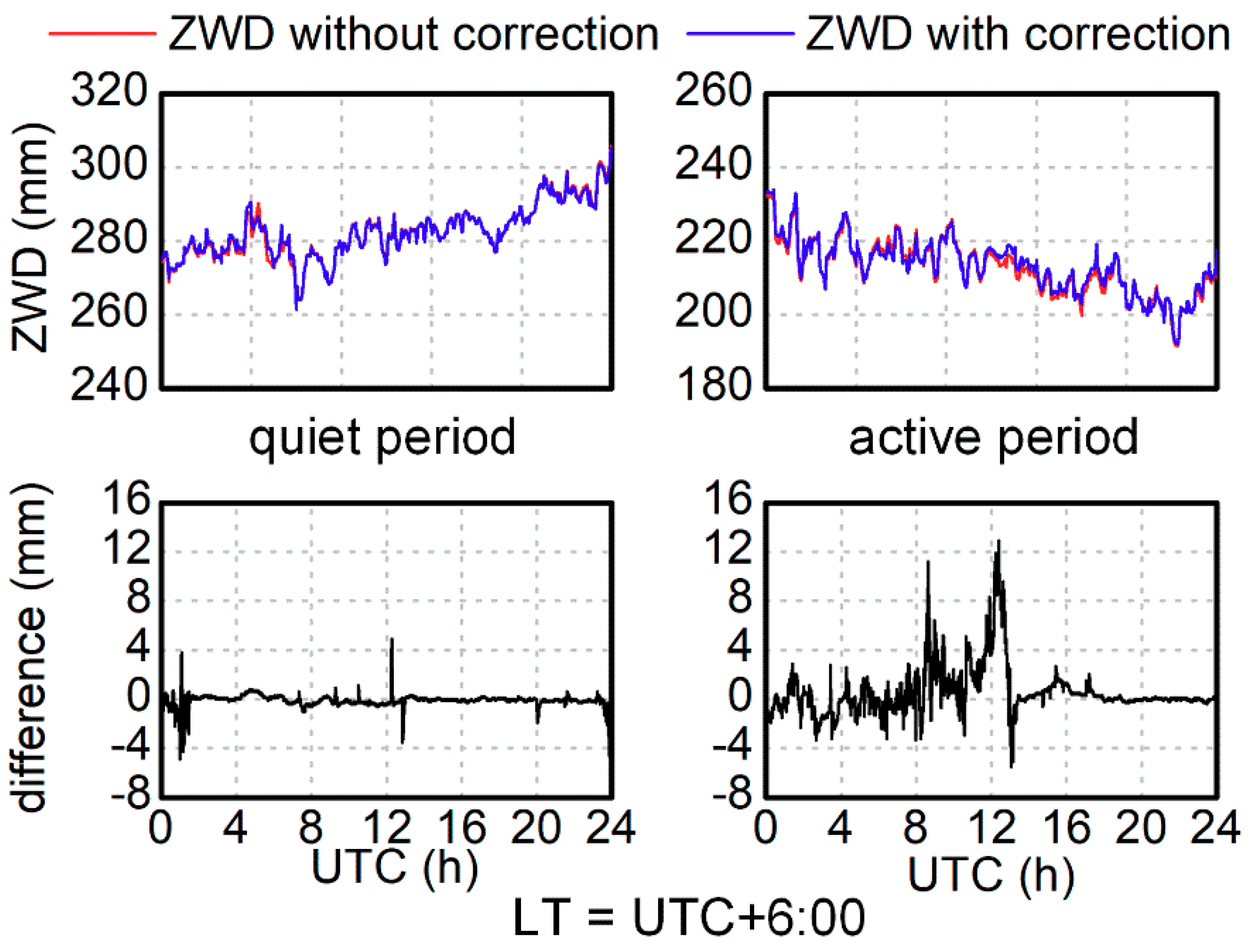
3.2. HOI Effects in Different Geomagnetic Conditions

To investigate the HOI effects on tropospheric delay estimation in different geomagnetic conditions, we obtained the ZWD estimates for stations located at different geomagnetic latitudes during active (geomagnetic storms, when Dst values reach up to –150 nT) and quiet periods (when Dst values fluctuate around 0 nT). The maximum influences of HOI on ZWD estimates during active and quiet periods, as well as their differences, are shown in Figure 9.

It can be seen that the effects of HOI terms on ZWD are highly correlated with geomagnetic latitude. The maximum ZWD differences are relatively small at high latitudes, and tend to become larger with decreasing latitude, reaching over 10 mm around the geomagnetic equator. Although energetic particles precipitate to the Earth through the poles, the effects of HOI is tiny at high geomagnetic latitudes for negligible changes in TEC values. Consequently, there is no statistically significant improvement in the estimation of tropospheric delays for stations at high latitude in a ZWD residual maximum sense. However, for stations located at low latitudes, the effects of HOI terms on ZWD estimation should be considered for precise atmospheric applications. Moreover, the different effects between the active and quiet periods shown in the bottom of Figure 9 further confirm that TEC is an important impact factor for ZWD estimation.

To allow a clearer comparison, the statistics of the effect of HOI on ZWD in different geomagnetic situations are shown in Figure 10. Absolute latitudes between 0 and 30° are defined as low latitudes, those between 30 and 65° degrees are defined as middle latitudes and those over 65° are defined as high latitudes. The statistical results show distinct differences between these three regions. The mean differences of ZWD estimation are about 7, 4, and 2 mm for the low, middle, and high latitudes, respectively. Additionally, the influences of HOI for the active period are slightly larger than those for the quiet period.

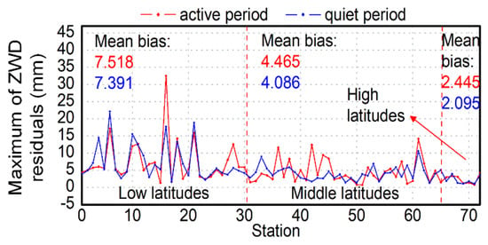
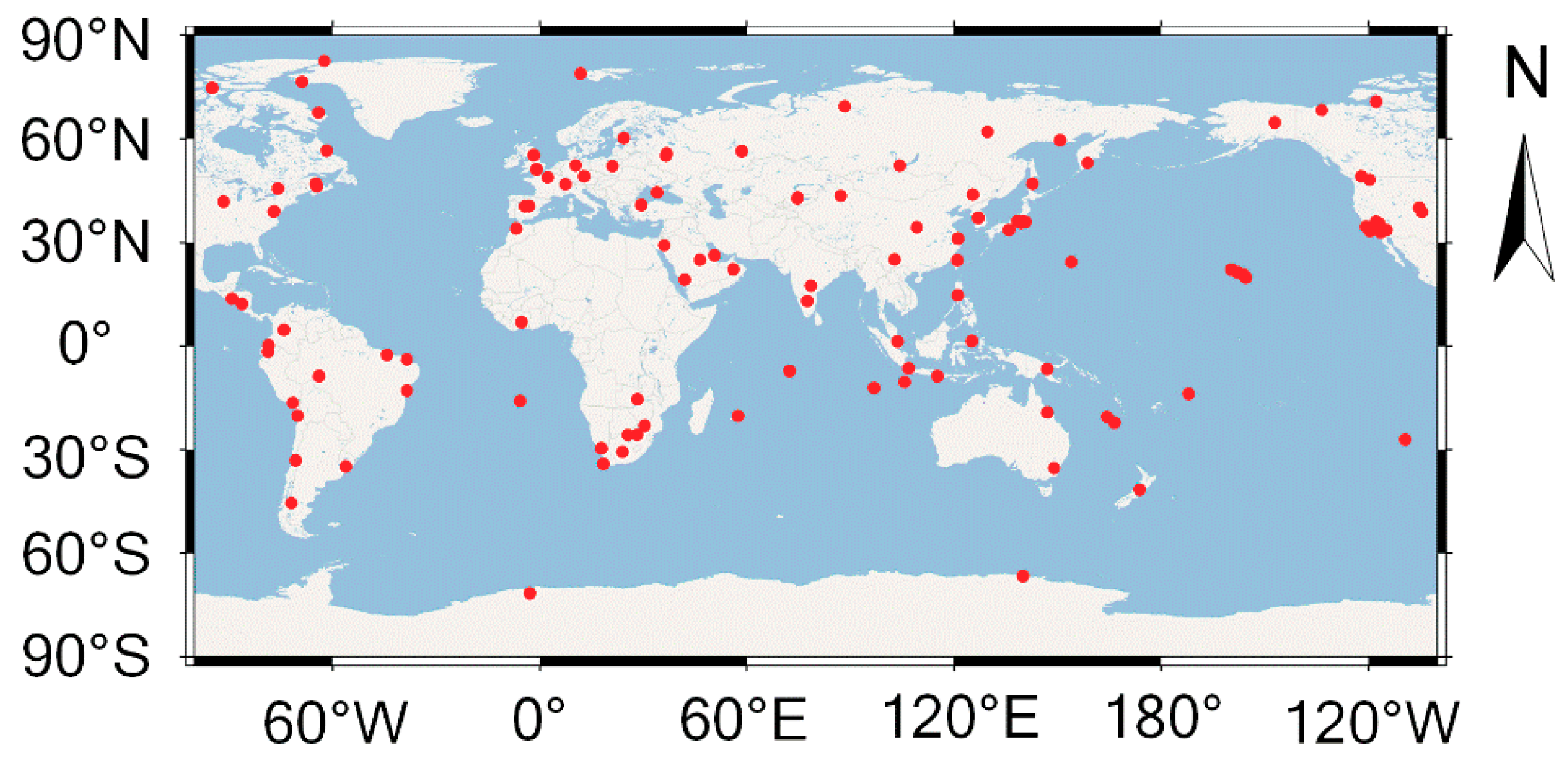
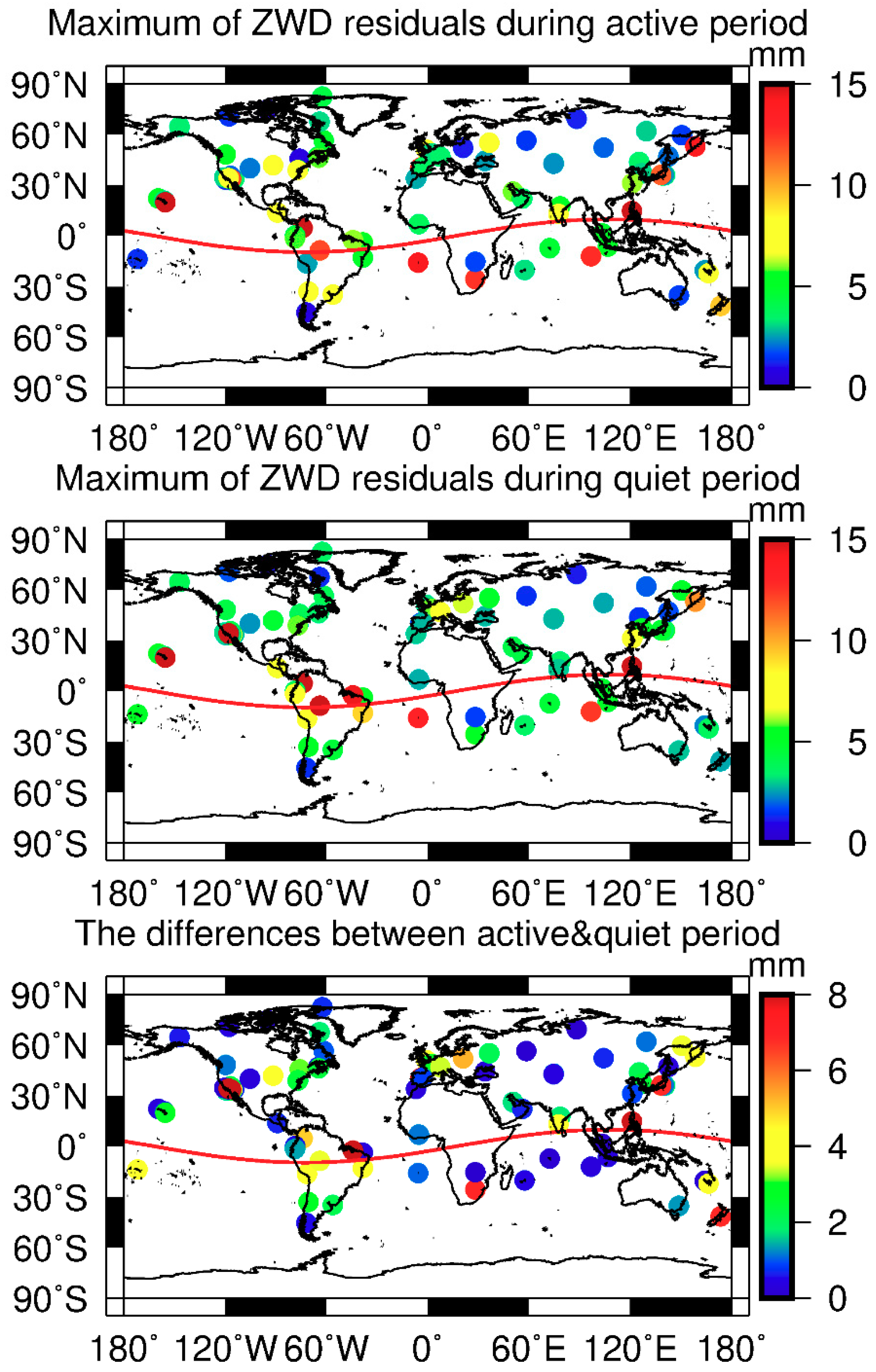
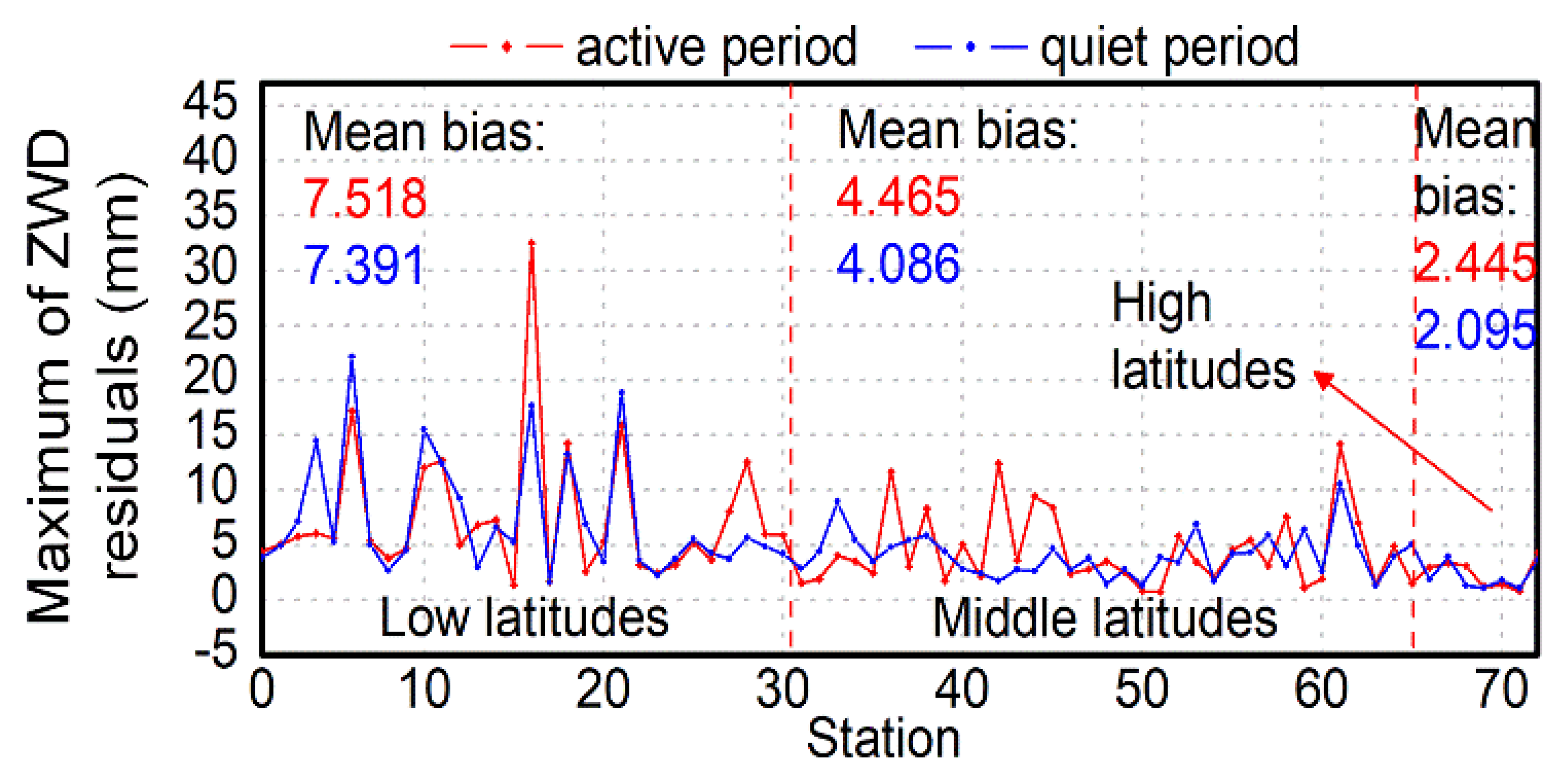
3.3. HOI Effects in Different Spatial Locations

The value of a HOI term depends on the interaction of the Earth’s magnetic field with electron density distribution along the raypath. Therefore, it varies with user position, elevation and azimuth angles, and it is difficult to assess the influence of HOI term on tropospheric delay estimation in a generalized way. In this section, we investigated the HOI effects of raypath in three-dimensional space with different azimuth and elevation angles. Tropospheric gradients were analyzed to describe the total effects of HOI terms for the raypath with different azimuth angles. Additionally, the correlation between slant tropospheric delay and elevation angle for a specific satellite–station link was investigated.

Figure 11 and Figure 12 show the estimated tropospheric horizontal gradients with and without HOI corrections, and their differences on MAUI station, which is located in the south of the geomagnetic equator, for quiet and active periods, respectively. As shown in Figure 11, almost no difference was noticed for the east–west (EW) gradients with and without HOI corrections during the quiet period, while the estimates of tropospheric north–south (NS) gradients were overestimated by 2–4 mm when the HOI terms were ignored. Figure 12 shows similar results, and it can be noticed that both the EW and NS gradients were slightly underestimated without HOI corrections. It should be noted that the unsmoothed differences which appeared in both directions during the active period may be caused by ionospheric disturbances. In general, the NS gradients are more likely to be affected by the HOI delays.

For almost all experimental data obtained from the equatorial anomaly area in our study, a similar effect to the one above can be observed. This effect can be explained by the raypath bending: When GPS signals traverse the equatorial anomaly area, significant raypath bending occurred, whereas the bending of signals travelling from other directions will be much lesser. For a station located around the geomagnetic equator, signals travelling along the direction of the geomagnetic field cause phase delays, while signals travelling in the opposite direction to the geomagnetic field lead to phase advances [29].

Figure 13 shows the impacts of HOI effect on slant tropospheric delay (STD), which can be derived from the ZWD estimates and mapping function. The sky plot, which clearly describes the change of satellite azimuth and elevation angle for the specific satellite (PRN 28), is shown as well.

As shown in Figure 13, the zero line divided the results into two separate parts, which represent the effects of phase advance and phase delay due to different ray locations in 3D space. Such differences arise from the variation of the angle between the raypath and the geomagnetic field. The changing of elevation angle not only affects the second-order ionospheric terms by influencing the angle $\theta$, but is also related to bending errors caused by the curved optical path. The combined effect of HOI term and signal bending on STD gradually changes with the elevation angle, and reaches up to 6 mm when the elevation angle is lower than 8°. Since the effects of bending errors are dominant over the HOI terms at low elevation angles, the major component of the combined effect is the bending errors.

4. Conclusions

This paper aimed to reveal the potential impact of HOI effects on GPS-estimated tropospheric parameters. For this purpose, a set of globally distributed stations was used for one month (from the day of year 237 to 257, 2017) for analysis, considering different ionospheric and geomagnetic conditions. HOI terms calculated from the correction model varied depending on the TEC level. The estimated ZWD with and without HOI corrections agrees well within 0.1 mm at night-time for both the ionospheric quiet and active periods, suggesting that the impacts of HOI effect on ZWD are marginal at night. However, in the daytime, the ZWD estimates differ by up to 4–5 mm and 12.9–21.3 mm for the ionospheric quiet and active periods, respectively, which should be carefully considered for precise atmospheric applications.

The influence of HOI terms on ZWD is highly correlated with the geomagnetic latitude and is approximately symmetrically distributed along the geomagnetic equator. On average, the maximum differences of ZWD estimation are about 7, 4, and 2 mm for the low, middle and high latitudes, respectively. As for the tropospheric horizontal gradients, no significant difference was noticed for the east–west (EW) gradients during quiet periods, while a difference of 1–2 mm was observed during active periods. Compared with the EW gradients, the north–south (NS) gradients are more likely to be affected by HOI delays. In general, the NS gradients were overestimated by 2–4 mm for both periods when the HOI terms were ignored.

References

1. Tregoning, P.; Boers, R.; O’Brien, D.; Hendy, M. Accuracy of absolute precipitable water vapor estimates from GPS observations. J. Geophys. Res. Atmos. 1998, 103, 28701–28710. [Google Scholar] [CrossRef] [Green Version]
2. Böhm, J.; Niell, A.; Tregoning, P.; Schuh, H. Global Mapping Function (GMF): A new empirical mapping function based on numerical weather model data. Geophys. Res. Lett. 2006, 33, L07304. [Google Scholar] [CrossRef]
3. Saastamoinen, J. Contributions to the theory of atmospheric refraction. Bull. Géod. (1946–1975) 1973, 107, 13–34. [Google Scholar] [CrossRef]
4. Hopfield, H.S. Tropospheric effect on electromagnetically measured range: Prediction from surface weather data. Radio Sci. 1971, 6, 357–367. [Google Scholar] [CrossRef]
5. Klobuchar, J.A. Ionospheric effects on GPS. Glob. Position. Syst. Theory Appl. 1996, 1, 485–515. [Google Scholar]
6. Hoque, M.M.; Jakowski, N. Estimate of higher order ionospheric errors in GNSS positioning. Radio Sci. 2008, 43, 1–15. [Google Scholar] [CrossRef]
7. Elmas, Z.G.; Aquino, M.; Marques, H.; Monico, J.F. Higher order ionospheric effects in GNSS positioning in the European region. Proc. Ann. Geophys. 2011, 29, 1383–1399. [Google Scholar] [CrossRef] [Green Version]
8. Wang, Z.; Wu, Y.; Zhang, K.; Meng, Y. Triple-frequency method for high-order ionospheric refractive error modelling in GPS modernization. J. Glob. Position. Syst. 2005, 4, 291–295. [Google Scholar] [CrossRef]
9. Brunner, F.K.; Gu, M. An improved model for the dual frequency ionospheric correction of GPS observations. Manuscr. Geod. 1991, 16, 205–214. [Google Scholar]
10. Bassiri, S.; Hajj, G.A. Higher-order ionospheric effects on the global positioning system observables and means of modeling them. Manuscr. Geod. 1993, 18, 280. [Google Scholar]
11. Petrie, E.J.; King, M.A.; Moore, P.; Lavallée, D.A. Higher-order ionospheric effects on the GPS reference frame and velocities. J. Geophys. Res. Solid Earth 2010, 115, B03417. [Google Scholar] [CrossRef]
12. Fritsche, M.; Dietrich, R.; Knöfel, C.; Rülke, A.; Vey, S.; Rothacher, M.; Steigenberger, P. Impact of higher-order ionospheric terms on GPS estimates. Geophys. Res. Lett. 2005, 32, L23311. [Google Scholar] [CrossRef]
13. Garcia-Fernandez, M.; Desai, S.; Butala, M.; Komjathy, A. Evaluation of different approaches to modeling the second-order ionospheric delay on GPS measurements. J. Geophys. Res. Space Phys. 2013, 118, 7864–7873. [Google Scholar] [CrossRef] [Green Version]
14. Elsobeiey, M.; El-Rabbany, A. Impact of second-order ionospheric delay on GPS precise point positioning. J. Appl. Geophys. 2011, 5, 37–45. [Google Scholar] [CrossRef]
15. Hernandez-Pajares, M.; Juan, J.; Sanz, J.; Orús, R. Second-order ionospheric term in GPS: Implementation and impact on geodetic estimates. J. Geophys. Res. Solid Earth 2007, 112, B08417. [Google Scholar] [CrossRef]
16. Deng, L.; Jiang, W.; Li, Z.; Chen, H.; Wang, K.; Ma, Y. Assessment of second-and third-order ionospheric effects on regional networks: Case study in China with longer CMONOC GPS coordinate time series. J. Geod. 2017, 91, 207–227. [Google Scholar] [CrossRef]
17. Hadas, T.; Krypiak-Gregorczyk, A.; Hernández-Pajares, M.; Kaplon, J.; Paziewski, J.; Wielgosz, P.; Garcia-Rigo, A.; Kazmierski, K.; Sosnica, K.; Kwasniak, D. Impact and Implementation of Higher-Order Ionospheric Effects on Precise GNSS Applications. J. Geophys. Res. Solid Earth 2017, 122, 9420–9436. [Google Scholar] [CrossRef]
18. Liu, Z.; Li, Y.; Guo, J.; Li, F. Influence of higher-order ionospheric delay correction on GPS precise orbit determination and precise positioning. Geod. Geodyn. 2016, 7, 369–376. [Google Scholar] [CrossRef]
19. Zus, F.; Deng, Z.; Wickert, J. The impact of higher-order ionospheric effects on estimated tropospheric parameters in Precise Point Positioning. Radio Sci. 2017, 52, 963–971. [Google Scholar] [CrossRef] [Green Version]
20. Douša, J.; Dick, G.; Kačmařík, M.; Brožková, R.; Zus, F.; Brenot, H.; Stoycheva, A.; Möller, G.; Kaplon, J. Benchmark campaign and case study episode in central Europe for development and assessment of advanced GNSS tropospheric models and products. Atmos. Meas. Tech. 2016, 9, 2989–3008. [Google Scholar] [CrossRef] [Green Version]
21. Marques, H.A.; Monico, J.F.; Aquino, M. RINEX_HO: Second-and third-order ionospheric corrections for RINEX observation files. GPS Solut. 2011, 15, 305–314. [Google Scholar] [CrossRef]
22. Schmid, R.; Steigenberger, P.; Gendt, G.; Ge, M.; Rothacher, M. Generation of a consistent absolute phase-center correction model for GPS receiver and satellite antennas. J. Geod. 2007, 81, 781–798. [Google Scholar] [CrossRef]
23. Wu, J.-T.; Wu, S.C.; Hajj, G.A.; Bertiger, W.I.; Lichten, S.M. Effects of antenna orientation on GPS carrier phase. Adv. Astronaut. Sci. 1992, 76, 1647–1660. [Google Scholar]
24. Budden, K.G. The Propagation of Radio Waves: The Theory of Radio Waves of Low Power in the Ionosphere and Magnetosphere, 1st ed.; Cambridge University Press: Cambridge, UK, 1988; pp. 328–356. ISBN 978-0521369527. [Google Scholar]
25. Davies, K. Ionospheric Radio, 1st ed.; IET: Stevenage, UK, 1990; pp. 89–124. ISBN 978-0863411861. [Google Scholar]
26. Rawer, K. Wave Propagation in the Ionosphere, 1st ed.; Springer Science & Business Media: Berlin, Germany, 2013; pp. 109–139. ISBN 978-9401736657. [Google Scholar]
27. Hoque, M.M.; Jakowski, N. Higher order ionospheric effects in precise GNSS positioning. J. Geod. 2007, 81, 259–268. [Google Scholar] [CrossRef]
28. Zus, F.; Deng, Z.; Heise, S.; Wickert, J. Ionospheric mapping functions based on electron density fields. GPS Solut. 2017, 21, 873–885. [Google Scholar] [CrossRef]
29. Kedar, S.; Hajj, G.A.; Wilson, B.D.; Heflin, M.B. The effect of the second order GPS ionospheric correction on receiver positions. Geophys. Res. Lett. 2003, 30, 1829. [Google Scholar] [CrossRef]
30. Odijk, D. Fast Precise GPS Positioning in the Presence of Ionospheric Delays. Ph.D. Thesis, Faculty of Civil Engineering and Geosciences, Delft University of Technology, Delft, The Netherlands, 2002. [Google Scholar]
31. Zumberge, J.; Heflin, M.; Jefferson, D.; Watkins, M.; Webb, F.H. Precise point positioning for the efficient and robust analysis of GPS data from large networks. J. Geophys. Res. Solid Earth 1997, 102, 5005–5017. [Google Scholar] [CrossRef] [Green Version]
32. Kouba, J.; Héroux, P. Precise point positioning using IGS orbit and clock products. GPS Solut. 2001, 5, 12–28. [Google Scholar] [CrossRef]
Figure 1. The distribution of International GNSS Service (IGS) stations used for analysis.
Remotesensing 10 01561 g001
Figure 2. The solar and geomagnetic index series from day of year (DOY) 237 to 257 in 2017. The solar storms occurred on DOY 247–249 and the geomagnetic storms occurred on DOY 250–252.
Remotesensing 10 01561 g002
Figure 3. Time series of Ion2 terms (top), Ion3 terms (middle) and vertical TEC (vTEC) (bottom) observed at station YKRO on DOY 239, 2017. The daytime (LT 12–17) and night-time (LT 0–5) are separated by a dashed line.
Remotesensing 10 01561 g003
Figure 4. The zenith wet delay (ZWD) estimates (top) with and without higher-order ionospheric (HOI) corrections and their differences with error bars (bottom) for station YKRO on DOY 239 in 2017 during the daytime and night-time.
Remotesensing 10 01561 g004
Figure 5. The distributions of ZWD differences for station YKRO during daytime (top) and night-time (bottom) on DOY 239 in 2017. The y-label “frequency” signifies the number of collected differences. The mean values and standard deviations of ZWD differences are shown in the top right corner of each figure.
Remotesensing 10 01561 g005
Figure 6. Time series of Ion2 terms (top) and Ion3 terms (bottom) of GPS L1 for station COCO on DOY 238 (quiet period, right) and 249 (active period, left) in 2017.
Remotesensing 10 01561 g006
Figure 7. The vTEC values for station COCO on DOY 249 in 2017 (active period) and DOY 238 in 2017 (quiet period). The daytime (LT 12–17) and night-time (LT 0–5) are separated by dashed lines.
Remotesensing 10 01561 g007
Figure 8. The ZWD estimates (top) with and without HOI corrections and their differences (bottom) for station COCO during the quiet and active period.
Remotesensing 10 01561 g008
Figure 9. The maximum influences of HOI on ZWD estimates during active (top) and quiet (middle) periods as well as their differences (bottom) for stations located in different areas. (Active period: DOY 250–252 in 2017, quiet period: DOY 241–243 in 2017).
Remotesensing 10 01561 g009
Figure 10. The statistics of the effect of HOI on ZWD in different geomagnetic situations (active period: DOY 250–252 in 2017; quiet period: DOY 241–243 in 2017). The mean biases of ZWD estimation differences in different ionospheric conditions are shown in the figure. Stations at different latitudes are separated by red dashed lines.
Remotesensing 10 01561 g010
Figure 11. The estimated tropospheric horizontal gradients (top) with and without HOI corrections and their differences (bottom) on station MAUI during the quiet period.
Remotesensing 10 01561 g011
Figure 12. The estimated tropospheric horizontal gradients (top) with and without HOI corrections and their differences (bottom) on station MAUI during the active period.
Remotesensing 10 01561 g012
Figure 13. The impacts of HOI effect on slant tropospheric delay (STD) (left) and the sky plot of PRN 28 (right) for station MAUI on DOY 249 in 2017. The phase advance and phase delay are separated by a black line.
Remotesensing 10 01561 g013