Article

Status of Aquarius and Salinity Continuity

1
NASA/Goddard Space Flight Center, Greenbelt, MD 20771, USA
2
Chapman University, Orange, CA 92866, USA
3
Remote Sensing Systems, 444 Tenth Street, Suite 200, Santa Rosa, CA 95401, USA
4
Earth and Space Research, 2101 Fourth Ave, Suite 1310, Seattle, WA 98121, USA
5
Jet Propulsion Laboratory, 4800 Oak Grove Drive, Pasadena, CA 91109, USA
*
Author to whom correspondence should be addressed.
Remote Sens. 2018, 10(10), 1585; https://doi.org/10.3390/rs10101585
Submission received: 5 September 2018 / Revised: 17 September 2018 / Accepted: 18 September 2018 / Published: 2 October 2018
(This article belongs to the Special Issue Sea Surface Salinity Remote Sensing)

Abstract

:
Aquarius is an L-band radar/radiometer instrument combination that has been designed to measure ocean salinity. It was launched on 10 June 2011 as part of the Aquarius/SAC-D observatory. The observatory is a partnership between the United States National Aeronautics and Space Agency (NASA), which provided Aquarius, and the Argentinian space agency, Comisiόn Nacional de Actividades Espaciales (CONAE), which provided the spacecraft bus, Satelite de Aplicaciones Cientificas (SAC-D). The observatory was lost four years later on 7 June 2015 when a failure in the power distribution network resulted in the loss of control of the spacecraft. The Aquarius Mission formally ended on 31 December 2017. The last major milestone was the release of the final version of the salinity retrieval (Version 5). Version 5 meets the mission requirements for accuracy, and reflects the continuing progress and understanding developed by the science team over the lifetime of the mission. Further progress is possible, and several issues remained unresolved at the end of the mission that are relevant to future salinity retrievals. The understanding developed with Aquarius is being transferred to radiometer observations over the ocean from NASA’s Soil Moisture Active Passive (SMAP) satellite, and salinity from SMAP with accuracy approaching that of Aquarius are already being produced.

1. Introduction

Aquarius is an L-band radar/radiometer instrument combination that has been designed to measure ocean salinity. It was launched 10 June 2011 and lost on 7 June 2015, almost four years to the day later when a failure in the power distribution network resulted in loss of control of the spacecraft. Mission operations ended soon afterward, and scientific operations (e.g., final algorithm) ended 31 December 2017. Aquarius was unique in that it was the only satellite dedicated solely to remote sensing of sea surface salinity (SSS). This manuscript reports an overview of the status of the Aquarius research on mapping the global surface salinity field as of the end of the scientific part of the mission on 31 December 2017. This overview begins with a short history and description of the mission (Section 2: Background). This is followed by a brief description of the salinity retrieval algorithm, Version 5.0, as it existed at the end of the mission (Section 3). A more detailed description of the algorithm can be found in Meissner, Wentz and Le Vine [1], and in this special issue [2]. Section 4 describes several of the important research issues that remain at end of the mission. This includes small residual changes in the temporal signal, a dependence on sea surface temperature (SST), and tuning of the calibration to improve the performance at the cold and warm ends. These “features” are hidden in Version 5 because they are either corrected empirically (temporal variations and SST-dependence) or are not manifested over the ocean (e.g., warm end occurs over land/ice). These features are pointed out here because further progress in improving the remote sensing algorithm requires a more fundamental understanding of the root cause of these issues. Finally (Section 5), the paper concludes with an introduction to the work that is continuing on the remote sensing of salinity from space using the observations of the SMAP L-band radiometer over the ocean.

2. Background

The Aquarius instrument is an L-band active/passive (radar/radiometer) combination designed to map surface salinity over the ocean [3]. It was part of the Aquarius/SAC-D observatory, which was a partnership between the United States National Aeronautics and Space Agency (NASA) and the Argentine space agency, Comisiόn Nacional de Actividades Espaciales (CONAE). Figure 1 is an artist drawing of the observatory. Aquarius consisted of three radiometers (the feed horns can be seen in the figure) arranged to image in pushbroom fashion looking toward the left with the spacecraft oriented as shown and flying perpendicular to the page (e.g., see Figure 3 in Le Vine et al. [3]). A NASA team from the Goddard Space Flight Center (radiometer) and the Jet Propulsion Laboratory (radar) built Aquarius. CONAE provided the spacecraft bus, SAC-D, and CONAE and its partners (Italy, France, and Canada) provided several other instruments [3,4] that are indicated on the Earth-viewing side of the bus.
Aquarius was unique among the recent L-band missions, (i.e., also the European Space Agency Soil Moisture and Ocean Salinity mission, SMOS, and the NASA Soil Moisture Active Passive, SMAP, mission) in that it focused exclusively on the measurement of sea surface salinity. For example, the radar was included to help correct for the effect of ocean surface roughness (waves), which is a major source of uncertainty in the salinity retrieval algorithm [5]. The radiometers were polarimetric (measured the third Stokes parameter) to provide an in situ measurement of Faraday rotation [6,7] that can be significant at L-band [8]. Even the orbit was chosen to optimize the retrieval of salinity. The orbit was sun-synchronous with a ground track close to the day–night terminator (18:00 equatorial crossing, ascending) so that the radiometer beams could look to the nighttime side to avoid the reflection of L-band radiation from the Sun into the antenna main beam (sun glint). In addition, the orbit was an exact repeat with a seven-day cycle that enabled Aquarius to view the same footprints each cycle to facilitate averaging to reduce noise in the measurement. The three radiometers provided sufficient coverage so that Aquarius mapped the globe completely in each seven-day cycle with overlap at higher latitude, again to facilitate averaging to meet the accuracy goal of 0.2 psu (global root mean square (RMS), monthly, and at 150-km spatial resolution [3]). The radar used the same feeds as the radiometer, but there was only one radar that was cycled among three feeds. The goal was to have almost simultaneous passive/active looks at the same spot on the surface.
Significant attention was paid to the thermal control of the instrument and included both active and passive elements. As part of the passive control, Aquarius carried a large thermal shield (the large umbrella-like shade separating Aquarius from the SAC/D spacecraft bus seen in Figure 1) to mitigate the effects of the Sun. There also was active thermal control to keep the critical parts of the radiometer at a stable temperature [3]. The requirement was for a variation of the radiometer front end of less than 0.1 °C per orbit, and the performance achieved on orbit was better than this [9].
Two other features new on Aquarius were the internal calibration and provisions for detection/mitigation of radio frequency interference (RFI). The internal calibration included reference diodes, and was the product of several years of research [10,11]. RFI was known to be a potential problem based on experience with airborne instruments [12,13], and provisions were made to address this problem. In particular, rapid sampling (10 ms per sample) and an algorithm to detect and remove pulses were implemented, because RFI at L-band from air traffic control radar was known to be a problem [3,14].
Aquarius released its first salinity map in September 2011 almost one month after it was turned on (Figure 5 in Le Vine et al. [9]), and functioned almost flawlessly and within specification until the observatory was lost on 7 June 2015. The problem was a failure in the power distribution network in the spacecraft. A component used in the power switches began to fail early in the mission. Since the switches were redundant, there was no early impact. Available information suggested a random failure mode, and that the probability of a failure in both primary and backup switch was small. However, in June 2015, power to the attitude control system was lost. Both primary and backup units had failed (the primary unit failed much earlier). Without attitude control, contact with the spacecraft was lost, and the retrieval of data was not possible. Operations ended soon thereafter, and the science team focused on consolidating its research for the release of a final version of the salinity retrieval. Version 5.0, the final Aquarius salinity product, was released in November 2017, and the Aquarius mission formally ended on 31 December 2017.

3. Results: Aquarius Version 5.0

This section provides a brief overview of the status of the final version, Version 5.0, of the Aquarius Project salinity retrieval algorithm. This includes the changes made to the algorithm, an assessment of its performance, and a list developed by the algorithm team at the end of the mission of issues that remained to be resolved.

3.1. Changes in the Retrieval Algorithm

The approach to calibration and the retrieval of salinity has not changed fundamentally since it was outlined in the pre-launch documentation [2,15,16]. However, changes have been made based on the actual data and the performance of the hardware on orbit. Each improvement led to better understanding of the calibration and algorithm, which in turn led to further improvements and further understanding. When significant changes were made to the retrieval, the data was reprocessed, and a new version of the salinity product was released to the public. In total, there were five versions (data releases). The changes are documented in a series of appendices to the pre-launch algorithm theoretic basis document (ATBD), which were issued with each new version of the algorithm to describe the changes incorporated in that version [16]. The changes made in the development of Version 5.0 are:
  • The ancillary sea surface temperature (SST) field was changed from the National Oceanographic and Atmospheric Administration (NOAA) Optimally Interpolated (OI) SST to the SST field from the Canadian Meteorological Center (CMC);
  • The reference sea surface salinity (SSS) field used in the sensor calibration and in the derivation of expected antenna temperature, TA_expected, in the forward algorithm was changed from SSS obtained from the Hybrid Coordinate Ocean Model (HYCOM) to the analyzed monthly Scripps Argo SSS;
  • The model for the celestial radiation reflected from the surface into the radiometer antenna was changed to values derived from fore and aft observations of the SMAP radiometer. The advantage of this approach is that it includes the effects of surface roughness;
  • The empirical symmetrization correction that corrects asc/dsc differences [1] was re-derived to reflect the improvements that resulted from the improved model for the reflected celestial radiation (above).
  • The model for absorption by atmospheric oxygen was changed from Meissner et al. [17] to the original model [18].
  • The surface roughness correction was updated (i.e., compared to that described in Meissner, Wentz and Riciardulli [19]):
    The SST dependence was adjusted.
    The dependence on significant wave height (SWH) was omitted.
    In addition, the correction table for dependence on wind speed and radar backscatter was updated, and as a consequence, the initial guess for the SSS field used to derive the final wind speed (i.e., “HHH” wind speed) was also updated.
  • Observations at vertical and horizontal polarization are given equal weight in the retrieval of salinity (i.e., in the maximum likelihood estimate used in the last step in the retrieval);
  • The L2 files include instantaneous rain rates based on the NOAA rain product, CMORPH (Climate Prediction Center Morphing). They are used to filter data for rain in the calibration and also for validating the Aquarius salinity versus in situ measurements.
Since Version 5.0 is the final version of the salinity retrieval for the Aquarius Project, it was decided to rewrite the ATBD to reflect the algorithm in place for Version 5.0 [1]. The data itself and a complete set of documents describing the algorithm can be found at the NASA Physical Oceanography Distributive Active Archive Center (PO.DAAC): https://podaac.jpl.nasa.gov/aquarius. Also, a description of the algorithm in its Version 3 form can be found in Boutin et al. [20]. The NASA PO.DAAC website also contains a historical record of the documents issued for each version (including evaluation metrics, users guide, and addenda to the ATBD).

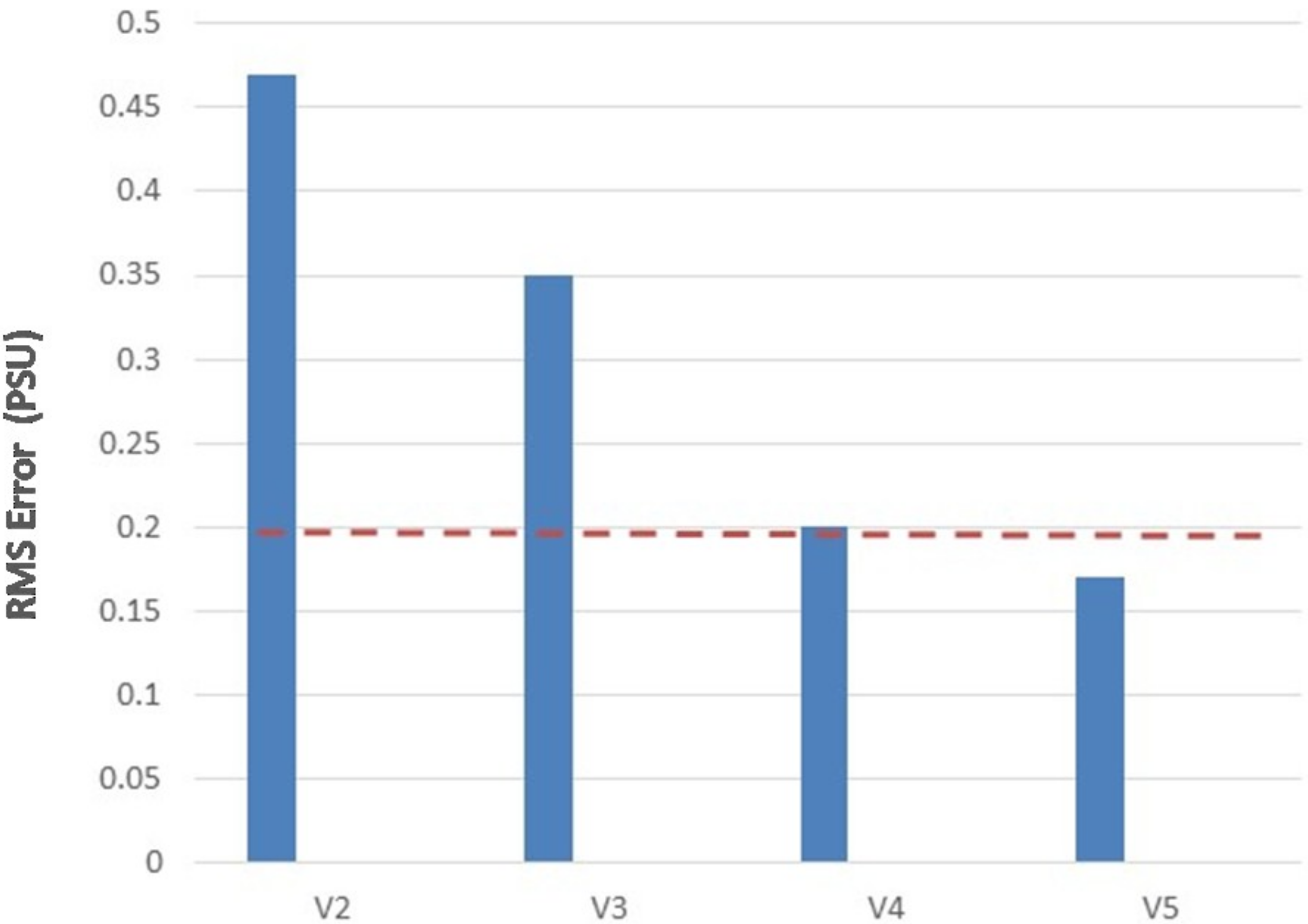
3.2. Evaluation of the Version 5.0 Salinity

The release of each Aquarius salinity product was accompanied by an evaluation of the product. The assessment is made by comparing the retrieved salinity with in situ measurements (mostly Argo floats [21]). In the matchup, Argo data closest to the surface is selected and matched to the nearest Aqaurius beam center within a search radius of ±3.5 days and 75 km. Then, 11 Aquarius observations (the data product is one salinity value every 1.44 s) are averaged centered on this point (see Kao et al. [22] for additional details). Figure 2 shows the RMS difference between the retrieved and in situ salinity averaged over the entire mission. The three bars represent the three Aquarius beams (beam 1 is the innermost beam), and results are shown for versions 2, 3, 4, and 5. The continuous progress and improvement in the algorithm since the early phase of the mission is evident in the gradual decrease in the level of error. The results shown for Version 5 (V5) are for the entire mission, and consist of individual matchups as described above, with no additional spatial or temporal averaging.
The statistics shown in Figure 2 include “error” in both the Aquarius retrieval and the error of the in situ measurements. The latter includes sampling error due to the relatively sparse in situ measurements and because they are not truly measurements at the surface (i.e., within the 1–2 cm where the microwave signal originates). In general, the discrepancy on the measurement depth between the satellite and in situ is negligible, but it could be a factor in the case of large precipitation and low mixing of the ocean upper layer [20]. One way to try to isolate the error in the Aquarius retrieval from the other sources is to use a triple-point analysis (e.g., see Appendix B in Kao et al. [22]). An example is shown in Figure 3 for beam 2 (the Aquarius middle beam). The data is the same as used in Figure 2. The dashed line represents the Aquarius mission requirement of an accuracy of 0.2 psu for the global RMS error on a monthly basis and a spatial resolution of 150 km. This triple-point analysis employs data from Aquarius, Argo [21], and the HYCOM [23] salinity field. The version of HYCOM used by the Aquarius project is the HYCOM + NCODA Global 1/12° Analysis (GLBA0.08, see https://hycom.org/data/glba0pt08). These data are not strictly independent. For example, HYCOM assimilates Argo data, so its SSS are not strictly independent from Argo measurements. However, HYCOM SSS are also affected by model ocean dynamics, evaporation–precipitation forcing, and a relaxation of HYCOM SSS toward a seasonal climatology (to prevent model drift). These factors tend to create some level of independence between HYCOM and Argo. Aquarius uses Argo during calibration (but not during retrieval). On the other hand, the data represent single comparisons, whereas the Aquarius requirement is for a monthly map. Since Aquarius maps the globe in seven days, one can expect four or more measurements in one month, and consequently, the monthly RMS is likely lower than the 0.17 psu shown in Figure 3 for Version 5.0. Calculations suggest the number is on the order of 0.13 psu (Table 4 in Kao et al. [22]).
Figure 4 is an example of the assessment of Level 3 (L3) data for V5 (L2 data is available in swath coordinates every 1.44 s, and Level 3 data is averaged into latitude and longitude bins of 1 degree × 1 degree resolution.) In Figure 4, the data are averaged for the entire mission [22]. The bars in each group represent different versions of the Aquarius salinity retrieval (V3, V4, and V5), and the groups show the data averaged spatially with increasing size, from the native one-degree to 10-degree bin sizes. Figure 4 illustrates two points: (a) the improvement in the retrieval with each new version, and (b) the impact of spatial averaging on reducing noise. It is evident from Figure 4 that V5.0 Level 3 exceeds the goal of 0.2 psu at 1o x1o and, as expected, improves with further spatial averaging.
The root mean square difference (RMSD) with respect to gridded Argo maps not only contains the errors of the Aquarius Level 3 SSS, but also the sampling and mapping errors of the Argo maps. The latter was found to be quite significant on 1° × 1° and 3° × 3° scales [24]; for example, the global average RMSD between two gridded Argo products is 0.1 psu on a 1° × 1° scale.

3.3. Work Remaining to Improve the Salinity Product

Aquarius Version 5.0 meets and exceeds the mission requirements. However, more can be done to improve the product. Among the issues identified by the Aquarius Cal/Val and Ocean Salinity Science Teams that will need to be addressed are:
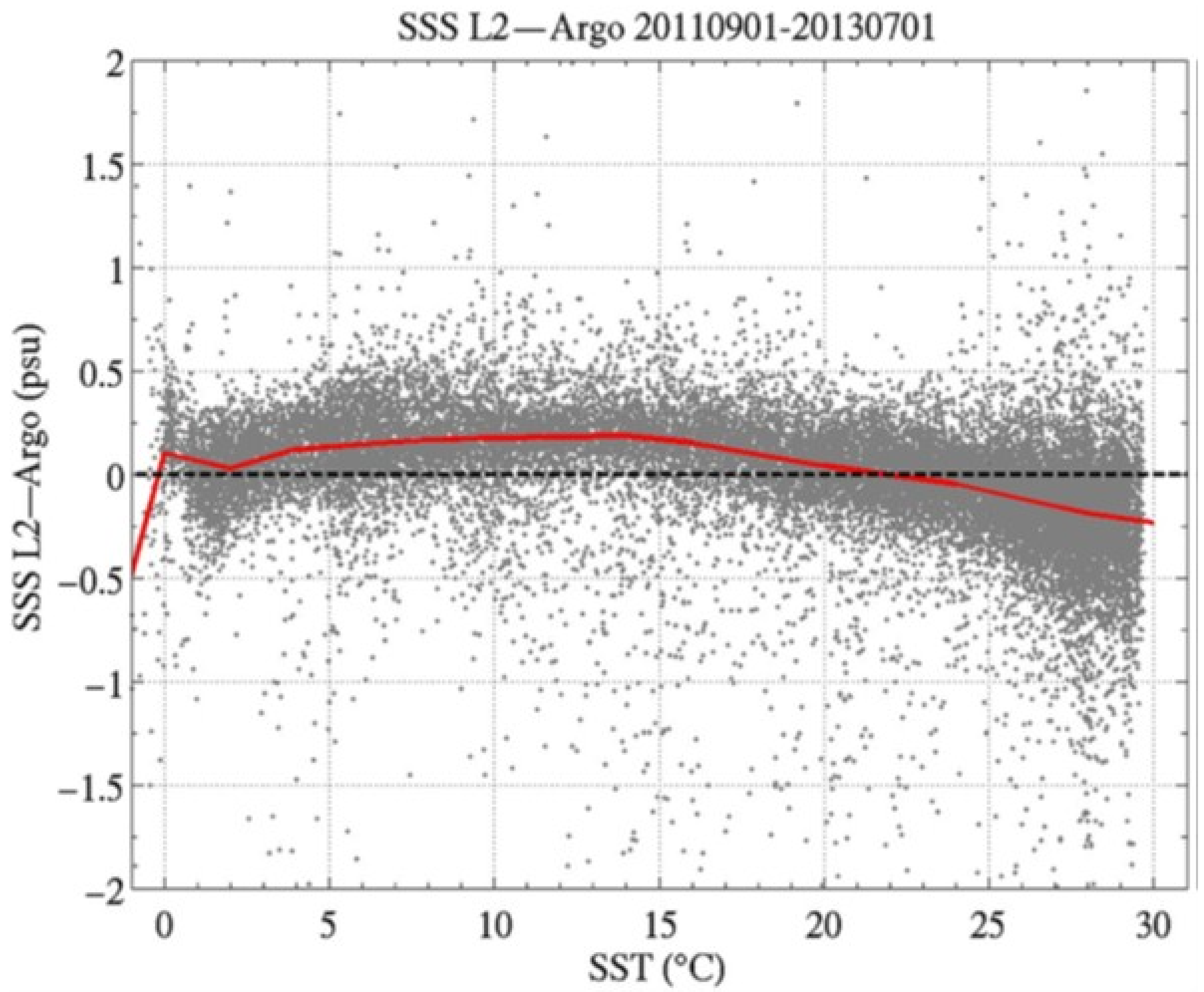
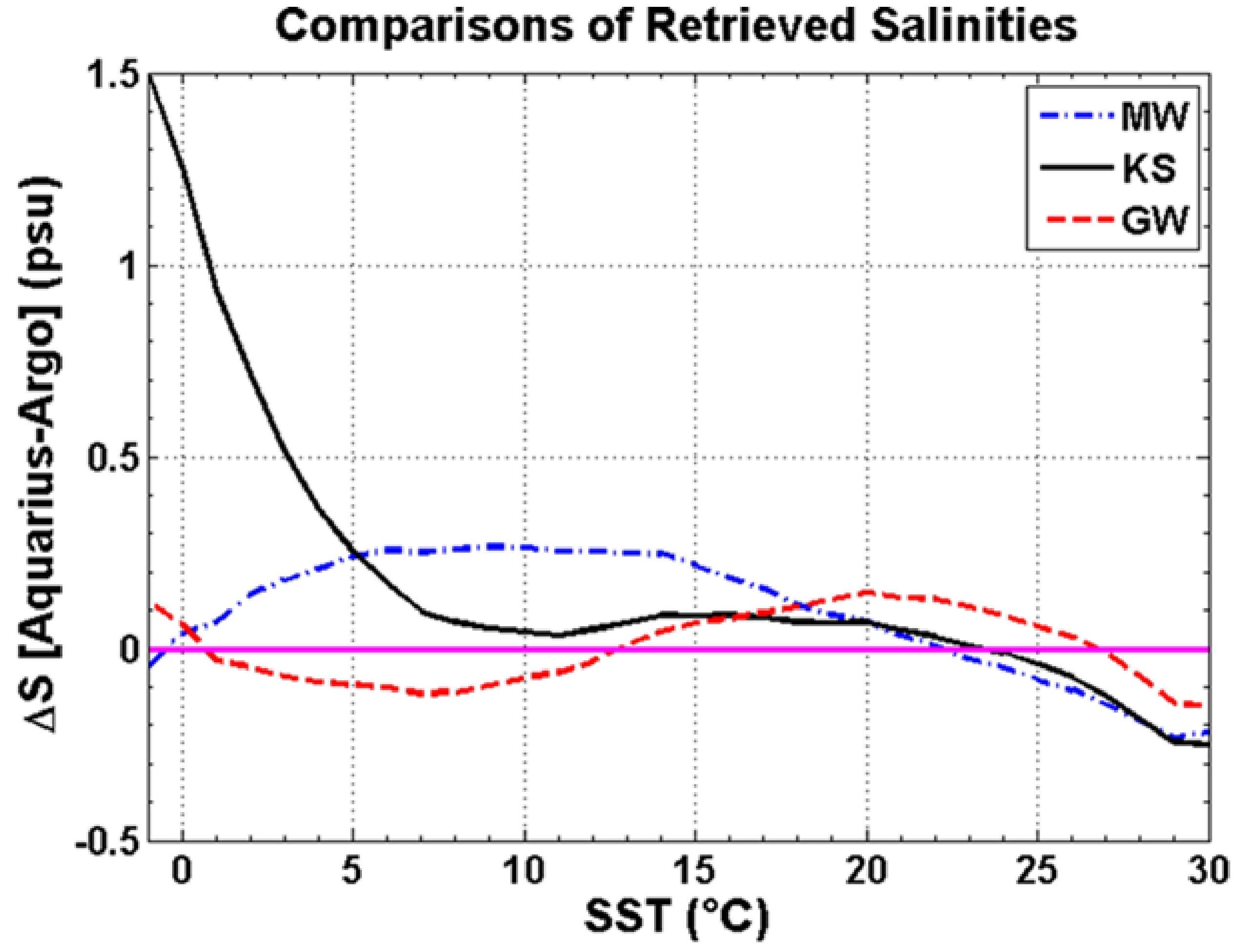
  • Determining the physical reason for an SST-dependent bias (which is empirically removed in Version 5; See Section 4.3 below);
  • Refining the model for the dielectric constant of sea water (i.e., functional dependence on SST and SSS), which varies among the two models currently in use, Klein and Swift [25] and Meissner and Wentz [26], and also the model being developed at the George Washington University [27];
  • Identifying and correcting a remaining small annual cycle (not due to changes in salinity);
  • Merging Aquarius, SMOS, and SMAP salinity maps into a single product;
  • Improving the theory for the effect of surface roughness on emission and the correction for the reflection of signals such as the galactic background;
  • Improving the level of missed detection in the RFI algorithm;
  • Improving the performance in cold water;
  • Addressing regional biases (e.g., North Pacific and southern Indian Ocean);
  • Improving calibration over the full range of expected targets (i.e., cold sky, ocean, and land).
The advantage of having a very stable instrument is that each improvement in the retrieval algorithm opens the door to additional possibilities. The manifestation of this can be seen in the steady improvement from Version 2 to Version 5 that is evident in Figure 2, Figure 3 and Figure 4. Examples are presented below to illustrate how this process unfolded for Aquarius for three of the issues listed above (SST-dependent bias, residual annual cycle, and calibration over the full range), and to describe the status of these issues as it exists in V5.

4. Discussion: Remaining Issues

4.1. Background

It helps for understanding the issues remaining in V5 to review, very briefly, two aspects of the salinity retrieval process: calibration (counts to TA) and the algorithm that converts the calibrated antenna temperature, TA, at the spacecraft to salinity at the surface.

4.1.1. Calibration

The internal hardware aspect of calibration (e.g., linearity correction, correction for temperature dependence, loss model, etc.) is based on pre-launch measurements and described in a summary document prepared for Version 5 [15]. The radiometers include internal reference sources (noise diodes) that are sampled periodically [11,15,28] and used to compute radiometer gain and offset. Although the values of the reference loads are measured pre-launch, an on-orbit check is required. In an ideal case, this should be a one-time check; however, (see “gain drift” below) the Aquarius radiometers were very good, but not perfect. In addition, largely because the antenna cannot be measured well enough on the ground, an on-orbit calibration of radiometer bias is necessary. In the case of Aquarius, the global average antenna temperature (which relies on ancillary salinity and temperature fields) is used as a reference for these external elements of the calibration, as will be explained in more detail below.

4.1.2. Retrieval of Salinity

Figure 5 is a schematic outlining the major steps in the transformation from the calibrated antenna temperature, TA, to the retrieval of salinity. Details can be found in the Aquarius ATBD, both the end of mission ATBD [1] and also the pre-launch ATBD and associated addenda [16]. The addenda were written to update the pre-launch ATBD to make it consistent with the revised processing each time a new version of the data was released. The end of mission ATBD is a rewrite of the ATBD to reflect the process in place for Version 5, which is the final Aquarius data set.
The retrieval of salinity consists of the transfer of TA from the spacecraft to the surface, and then the calculation of surface salinity. Figure 5 illustrates the major steps in going from TA to the brightness temperature at the surface. These are in order (yellow boxes): off-Earth sources (e.g., the Sun) are subtracted; a correction is made to account for antenna imperfections; a correction is made for Faraday rotation (which changes the polarization) and for attenuation and emission from the atmosphere; then, the brightness temperature is corrected for surface roughness (e.g., waves that are parameterized as a function of wind and normalized radar cross-section); and finally, the SST is used with a model for the dielectric constant of sea water to retrieve SSS. The path shown in Figure 5 is used in two ways: to compute salinity from calibrated TA, and in reverse to compute TA from the known values of salinity. The latter is called “expected TA” in the Aquarius literature, and is used in the calibration of the radiometer. In particular, the upward version of the algorithm evaluated over reference scenes is used to predict the value of antenna temperature that is expected at the radiometer output. This is compared with the actual value as part of calibration. In essence, calibration consists of matching what is measured and “expected” TA (called TA_expected). This was done once after the radiometer was first turned on in orbit to adjust the radiometer bias and set the value of the reference noise diode. In addition, this was done periodically with the radiometer looking at cold sky to check for stability [29]. It was also done while looking at the ocean and using a salinity reference model (e.g., the ocean model HYCOM or a set of in situ observations such as from the Argo floats) to fine-tune gain and offset (see “drift and bias” below).

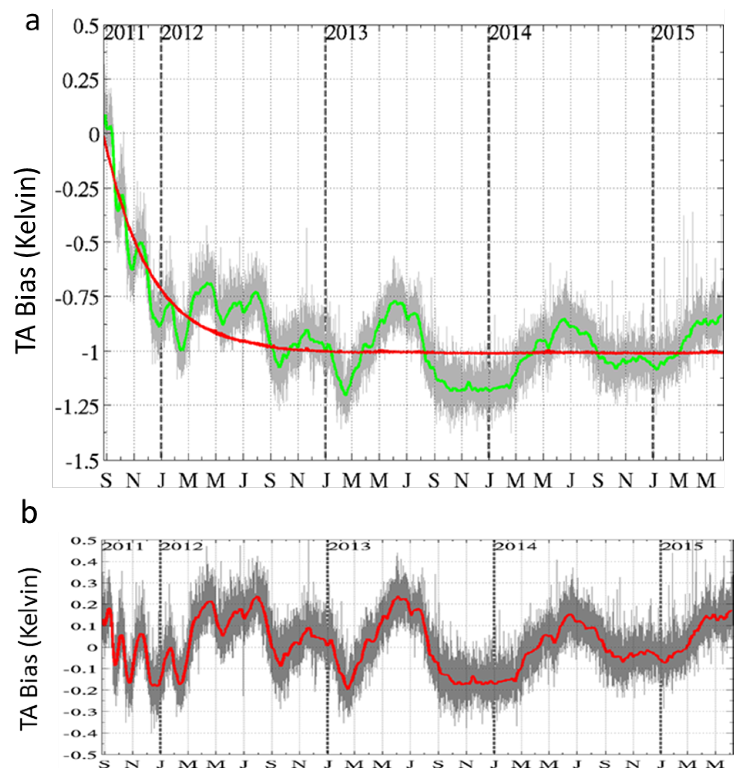
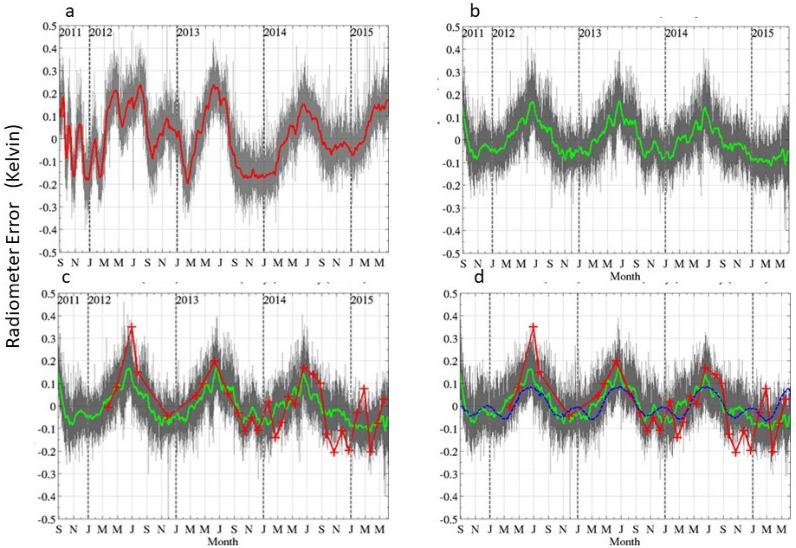
4.2. Example Issue: Drift and Wiggles

After the initial on-orbit calibration to establish the value for the reference noise diode and bias [15], the radiometer performance was monitored by comparing the global average TA (over the ocean) with the TA_expected using surface salinity from HYCOM. In Version 4, some regions with known issues (e.g., RFI and ice/land contamination) were eliminated to form a more reliable calibration subset. In Version 5, areas with rain were added to this list, and in addition, the reference salinity was changed to the Scripps optimally interpolated Argo salinity field [30].
Figure 6a shows the time history of the difference, TA—TA_expected, as it looked at the end of the mission [29]. The grey shows the difference per orbit, and the green curve is a seven-day average (sliding window). Red is an exponential fit to the data. The vertical axis is the difference (Kelvin), and the abscissa is time (months) since the beginning of data collection (Aquarius was turned on in August 2011) until the end (June 2015). The total change is small, but this must be considered in the context of the requirements for measurement of salinity (a sensitivity of about 0.5 K/psu and accuracy goal of 0.2 psu). There was great concern at the beginning of the mission with the (relatively) rapid change (i.e., the decrease evident in Figure 6a during the first three months of the mission). However, the exponential nature of the change soon became clear, and based on the leveling of the change, it was assumed that some manner of outgassing was the cause. It was decided to model this feature with an exponential and remove it as part of calibration. The correction was made by adjusting the temperature of the reference noise diode [31].
Figure 6b shows the same data after correction for the exponential drift (the scale is the same as in Figure 6a to make the comparison easier). The irregular “oscillations” around zero were given the name, “wiggles”, by the Aquarius team for want of a better name. They remained a mystery for some time. However, around the time that V4 was being prepared, it was discovered that a potential source for this behavior was an instability in the radiometer backend voltage to the frequency converter [32]. A model for the behavior was developed based entirely on the radiometer hardware, and the model was used to make a correction for this feature in Version 5 (it was first employed in Version 4).
Figure 7 shows the corrected difference (beam 1, horizontal polarization). Figure 7a is the same as Figure 6b and Figure 7b is the residual, TA—TA_expected, after correction for the backend instability. Again, grey is the difference per orbit, and green is a seven-day average. The instrument-only correction reduced the “wiggles”, but did not remove them. This correction also dramatically changed their character. There is a very clear annual cycle in the residual after this correction. The grey and green curves are data collected in the nominal mode: viewing ocean. The red curve in Figure 7c shows the difference calculated for data collected when looking at cold sky and superimposed on the data in Figure 7b. The crosses “+” indicate the actual data points. It is evident from Figure 7c that this behavior is not scene-dependent, and therefore, it is most likely not associated with an error in the radiative transport model of the ocean used to compute the grey and green curves. The shape of the curve and, in particular, the small hump between the larger peaks is suggestive of the solar beta angle (Figure 7 and Figure 8 in Dinnat and Le Vine [33]), which suggests a potential correlation with instrument temperature. The blue curve in Figure 7d shows the temperature of the reference noise diode shared by the two polarizations (i.e., correlated noise diode [3]) centered on zero (i.e., mean value over mission lifetime subtracted). An effort was made to find a connection between temperature variations and the residual in Figure 7. For example, temperatures were varied in the radiometer loss model [15], and although changes were observed in TA, it was not possible to reproduce changes of the order of magnitude that was seen in the data.
The source of the residual shown in Figure 7 remains unknown. It is corrected empirically in Version 5. This was done by calculating the difference, TA—TA_expected, and averaging using a seven-day sliding window (i.e., seven days centered on the current time). This average difference is treated like a bias and subtracted from TA. This removes the artifact from the retrieval of salinity; however, the annual signature strongly suggests a physical cause which, if identified, will lead to better understanding and likely a better salinity product.

4.3. Example Issue: SST Dependence

During the research leading to release of Aquarius Version 3.0, regional biases were observed in the error of the salinity retrieval. The bias had a strong zonal behavior, with salty biases noticed in mid-high latitudes, and fresh bias in the tropics and subtropics (see Section 6 of Addendum III of [17,34]). The zonal character of those biases suggested a correlation with SST, which was confirmed, and Version 3 was released with both a nominal version and an option for the removal of an SST-dependent bias (e.g., see Addendum III in the Aquarius ATBD [16]).
Figure 8 shows an example of the SST dependence. The vertical axis (ordinate) is the difference between the retrieved salinity and the value reported by Argo floats, and the abscissa is SST. The grey are individual differences, and the red curve is the median value. The matchup is with a smoothed map of Argo values formed by binning the near-surface Argo observations. Notice the fresh bias at very warm temperatures, which is typical of the tropics and low latitude, and the salty bias, which is typical at cooler temperatures and higher latitude. The behavior at very cold temperatures is different and an issue of its own (see below). The data in Figure 8 are from Version 3 of the algorithm. This choice was made because in versions 4 and 5, empirical adjustments have been made that hide the extent of the dependence on SST.
The reason for the SST dependence of the error is not known, but it is likely associated with the residual errors in one of the geophysical model functions used in the SSS retrieval algorithm. The most probable candidates are the model function for the dielectric constant of sea water (which has a strong dependence on SST) and the model for atmospheric absorption and emission, which has a latitudinal dependence. A temperature dependence was also included in the empirical model that is employed to correct for the effect of surface roughness on emissivity (e.g., Section 2 of Addendum III of the Aquarius ATBD [16]), which is somewhat arbitrary and not necessarily physically correct.
In the research leading to the release of Version 5.0, the model used in previous versions for attenuation by oxygen was identified as a contributor to this bias. The problem appeared to be with a modification made to the Liebe model for the effect of oxygen in the calculation of atmospheric absorption. In Version 5, this modification was abandoned in favor of the original model [18].
The return to the original Liebe model in Version 5 improved the performance of the algorithm at high latitude and decreased the SST dependence. The remaining SST bias is removed empirically in Version 5 by empirically adjusting the temperature dependence in the correction for roughness [1]. In Version 5, an additional temperature dependence is added to the correction of emissivity for roughness (e.g., Equation (13) in Appendix V of the end of mission ATBD [1]) and adjusted empirically). As a consequence, Version 5.0 is able to remove the SST-dependent bias to within ±0.1 psu, even in cold water.
This empirical adjustment of the roughness correction is an effective solution, but it does not give insight into the physical source of the SST dependence. In particular, it clearly depends on the model function that is used for the dielectric constant of sea water. This is illustrated in Figure 9, which shows the dependence of the salinity error on SST when different model functions are used in the retrieval from Aquarius brightness temperature to SSS. The solid black curve is the Klein–Swift model function [25], which is used by SMOS. The dashed blue curve is the Meissner–Wentz model function [26,35], which is used in the retrievals by the Aquarius Project, and the dashed red curve is the model function reported by Zhou et al. [27], and based on their measurements at 1.413 GHz [36,37]. The models by Klein and Swift and Meissner and Wentz have been used in the SSS retrievals by various teams using SMOS, SMAP, and Aquarius brightness temperature. The model by Zhou et al. is more recent, and has not yet been used in SSS products.
Figure 9 was obtained by keeping the retrieval algorithm fixed and replacing the dielectric constant with one of the three model functions. The example in Figure 9 was produced using Version 3 of salinity retrieval, because changes were made in V4 and V5 that empirically corrected for the SST-dependent bias, and are hard to remove. It is evident that the dependence of error on SST is different for the three model functions, especially at very low temperatures. It is also clear from Figure 8 that there is an issue with the retrieval at temperatures near 0 °C (although the data are sparse at these temperatures), and Figure 9 shows a very different and inconsistent dependence on the model function that is used in the retrieval at low temperatures. This is an especially important issue because of the importance of cold water with changing climate (i.e., understanding the effect of melting ice and the associated in flux of fresh water on ocean circulation) and because cold water is also a region of decreased sensitivity to changes in salinity (e.g., Figure 2 in Le Vine, Lagerloef and Torrusio [38]).
As mentioned above, the SST dependence is removed in Aquarius Version 5 by correcting the model for atmospheric absorption, which reduced the bias, and then empirically removing the residual bias. The empirical fix is good at removing the SST dependence; however, there are likely physical causes for this dependence, such as the model function for the dielectric constant of sea water, which when more fully understood will lead to improved retrievals in the future and lessen the need for empirical adjustments.

4.4. Example Issue: Whole Range Calibration

4.4.1. Introduction

The goal of Aquarius is to measure sea surface salinity in the open ocean, and the calibration of the instrument has been tuned to achieve this goal. There are two calibration scenes that are sufficiently large and uniform, and sufficiently well-known to be appropriate for this purpose: cold sky and the ocean itself. Both have been used in the calibration of Aquarius, but after the initial removal of a bias, the calibration uses only the ocean (e.g., see discussion of drift above). After the initial post-launch check for bias, the cold sky was used only to look for temporal changes as a check on stability and adjust the model for the antenna patterns [29].
In the ideal case, the Aquarius calibration would use two points (e.g., cold sky and ocean) and be checked at a third (e.g., land). Even better, the calibration would use cold sky and a non-ocean scene such as land or ice, and then be verified over the ocean. Unfortunately, this is not practical, because scenes at the warm end (e.g., 250 K which is typical of land and ice at L-band) are generally not known with sufficient accuracy over a large enough area to be compatible with the Aquarius footprint (3-dB radius on the order of 100 km [3]). Furthermore, because the brightness temperature of the open ocean at L-band has a very limited dynamic range, it is possible to have a calibration that is accurate over the ocean, but not sufficiently accurate at the warm extremes for applications over land such as the retrieval of soil moisture. This is illustrated in Figure 10, which shows a plot of the measured Aquarius antenna temperature, TA_meas, against the expected value computed given the appropriate surface truth (salinity and water temperature for ocean). The data are for the horizontal polarization and the middle beam, and the dashed line is the Aquarius calibration curve. The insets show expanded views over the ocean and at cold sky. It is clear that the calibrated operating curve for the radiometer (dashed line) is well fitted to the ocean data, but that the radiometer is too cold at the cold end (inset for cold sky, magenta) and is too warm at the warm end (red dots near 250 K). The data at the warm end at 250 K are from measurements over the United States Department of Agriculture (USDA) Little River research watershed.

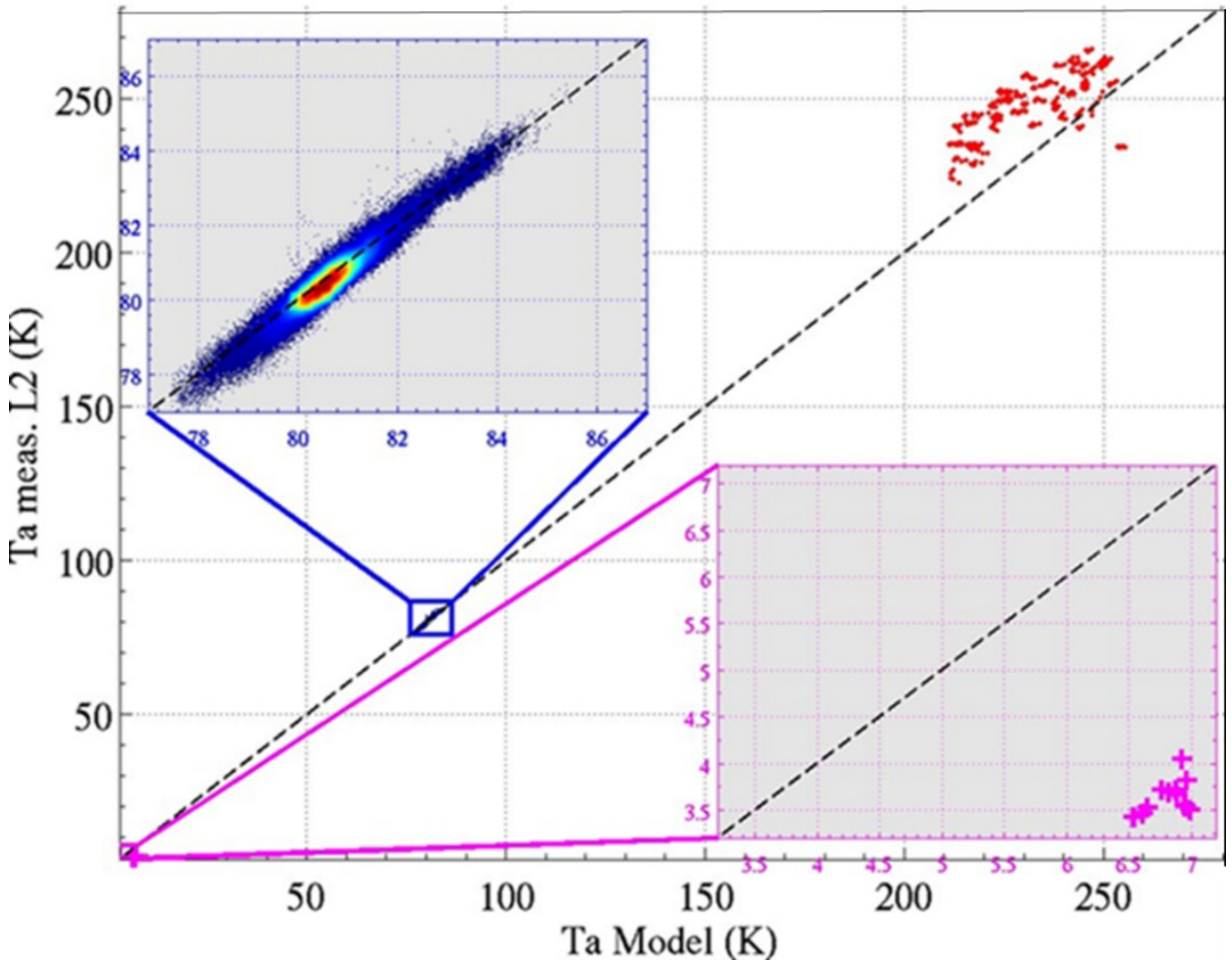
4.4.2. Whole Range Calibration V5.WR

An initial attempt has been made in Version 5 to provide a better calibration for the full range of applications by including the cold sky in a two-point (cold sky and ocean) calibration. Essentially, this amounts to drawing a straight line between these two references, and extending it to warm brightness temperatures [39]. This calibration is provided as an extension of Version 5, and called Version 5.WR [40,41].
The development of Version 5.WR begins with V5, and adds an additional step in which the cold sky and ocean observations (V5) are used to tune the calibration. The change is a linear transformation from the original V5 antenna temperatures to the new, V5.WR antenna temperatures: TA_V5.WR = a TA_V5.0 + b. The large difference in antenna temperature between cold sky (4 K) and ocean (80 K) helps determine the slope as a function of the target TA in a way that is not possible with only ocean observations, which have a small dynamic range (e.g., see the insets in Figure 10). The changes have minimal effect on the data over ocean or the retrieved salinity [40], because the ocean global average TA is kept unchanged by design.
The coefficients (a, b) are given in Table 1. They were derived from a linear regression between two points as follows:
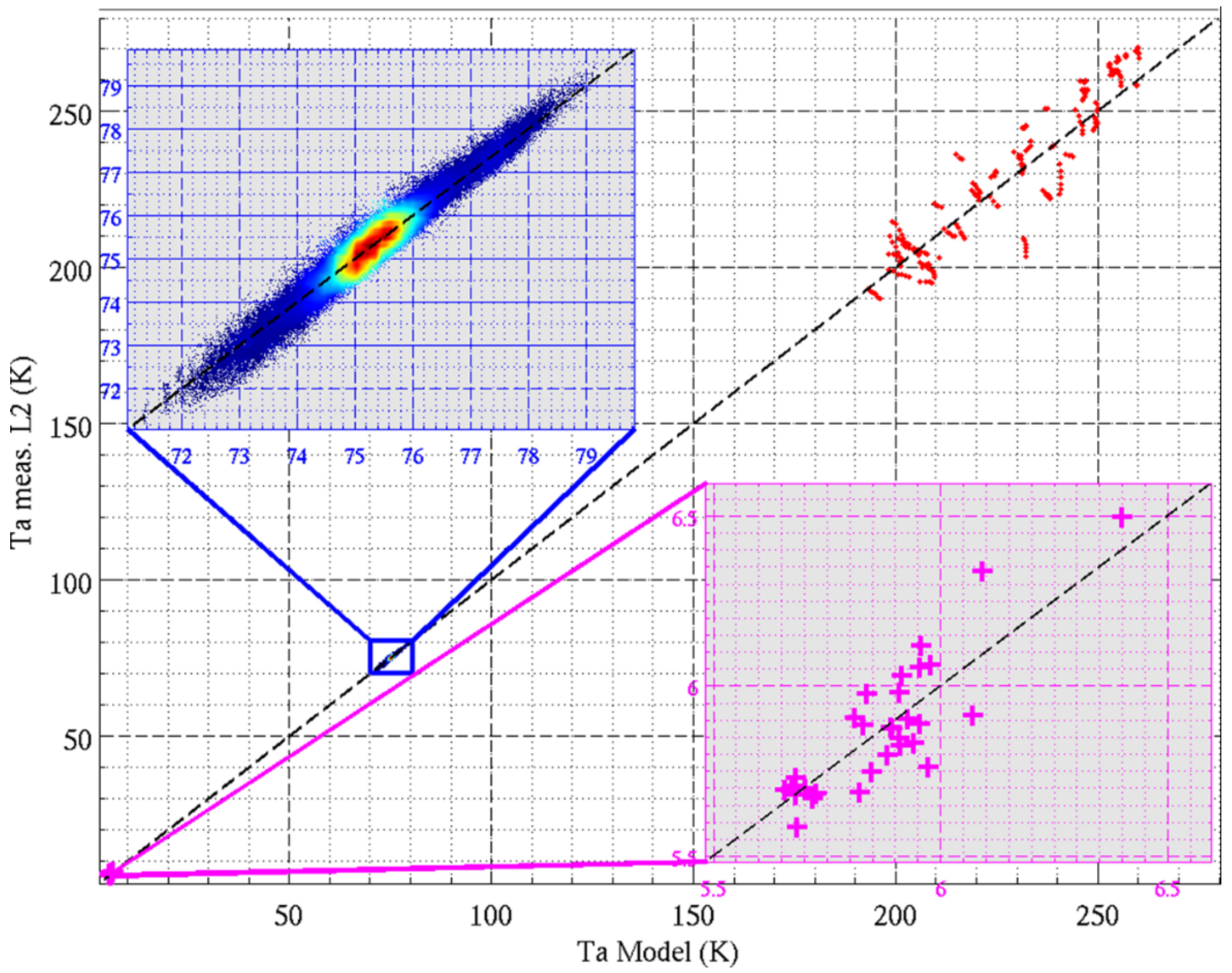
  • At the cold end, using the difference between the mean of the TA measured by Aquarius for the 30 cold sky calibrations and the mean of the corresponding TA_expected for the cold sky look computed from radiative transport theory;
  • Over the ocean, using the mean of the TA measured by Aquarius globally for the year 2012 (filtered for RFI, and with a water fraction of ≥99.9% ) and the mean of the corresponding TA_expected.
A full evaluation of the whole range calibration, V5.WR, is not complete, largely because of the lack of reference sites of sufficient size, but a check has been made over the USDA Little Washita and Little River watersheds, which are instrumented for monitoring soil moisture, as shown in Figure 11. Due to the large footprint and fixed orbit of Aquarius, it was not possible to use the same scene for all of the beams. The improvement compared to earlier versions of the algorithm without the whole range calibration is evident by comparing it with the example in Figure 10. The improvement at the cold end is significant. The change over land when compared with V5 is an improvement by as much as 2.2 K (H-pol and outer beam), and generally on the order of 1 K. These changes are small compared to the uncertainty in the model due to uncertainties in the surface truth (soil moisture) and effect of vegetation, and the small size of the scene compared to the footprint of the radiometer. Further validation of the results at the warm end is needed. Due to this, and to avoid confusion with V5, the version V5.WR has not been listed in the public database; however, it is available to the public upon request from the PO.DAAC.

5. Conclusions: Future of SSS Remote Sensing

Although the Aquarius mission has ended, research on the remote sensing of sea surface salinity from space by NASA continues by shifting the effort of retrieving SSS to SMAP. This work actually started several years ago within the Aquarius project. Soon after SMAP was launched, a subset of the Aquarius science team submitted a proposal to NASA to look at the feasibility of adapting the Aquarius salinity retrieval algorithm to retrieve salinity using the SMAP radiometer observations over ocean. Retrieving salinity from SMAP presented several obvious challenges. (1) The SMAP radar failed soon after launch, which means that a model function and external source for wind speed are needed for the roughness correction. (2) The loss and temperature dependence of the SMAP antenna system are not well-known (compared to Aquarius), which requires addition empirical adjustments that are not necessary with Aquarius. The objective of this work was to transfer the algorithm and understanding gained with Aquarius to SMAP data to see if a scientifically meaningful SSS product could be obtained.
The work with SMAP data began during the Aquarius project, and initial results have been reported [42,43,44]. Figure 12 is an example. Figure 12a shows the mean salinity field from SMAP data reported by remote sensing systems [44] from algorithm Version 2 (based on Version 3 of SMAP Level 1B brightness temperatures) for the two years 2015–2016. The dominant features of the global surface salinity field are clear (the Atlantic Ocean is saltier than the Pacific; dipole-like structure with salty mid-latitudes separated by the fresher tropical convergence zone; salty Arabian Sea; fresher Indian Ocean). However, there is clearly work to be done to improve the overall performance of the retrieval. This is illustrated in Figure 12b, which shows the salinity error map (the difference between the retrieved SSS and in situ measurements from Argo). A notable feature is the strong zonal dependence with salty bias (positive) in the low latitudes and fresh bias (negative) at mid and high latitudes. Plotting the error as a function of temperature demonstrates an SST dependence that is just the opposite of that present in Aquarius V5. (The SMAP V2 salinity retrieval uses the same model function as Aquarius V4, which suggests that this difference is due to something that is specifically associated with SMAP such as the external wind speed that goes into the roughness correction, or the loss model for the reflector model, or both.)
Now that the Aquarius Mission has ended, plans are in place to build upon this structure to form a NASA salinity continuity project using SMAP data. A new ocean salinity science team is being formed to work on this data. It will include research at the Jet Propulsion Laboratory and Goddard Space Flight Center, and a nominal algorithm with processing the responsibility of remote sensing systems (which was responsible for the Aquarius algorithm). Data will be available at the PO.DAAC, and there will also be an independent website (https://salinity.oceanscience.org) with information for the public and links to other data products, similar to what was available for Aquarius.
An important part of the work on Aquarius was the assessment of the data product. This meant matching in situ measurements with the retrievals from space, and taking into account the error of the pointwise in situ measurements to represent the salinity values on Aquarius’ measurement scales. It is planned to continue this work and cooperate with the effort that is currently underway at the European Space Agency (ESA) to develop a matchup database to support salinity retrievals of SMOS [45]. Hopefully, a common database for this purpose can be developed that helps in the evaluation and eventual merging of the two sources of salinity observations.
Finally, work is underway to prepare for the future. Aquarius is gone, and SMOS is aging. SMAP is already nearly four years old. At least two missions with L-band radiometers are under development in China [46,47,48], and one of them, the Water Cycle Observation Mission (WCOM), is scheduled for launch in the near future [47]. Studies are also underway within NASA, at the Jet Propulsion Laboratory (JPL) and the Goddard Space Flight Center (GSFC), to define the NASA L-band mission of the future. Designs for broadband sensors including lower frequencies such as P-band and with and without radar have been reported [49,50]. However, this is preliminary design, and the optimum choice is far from clear [32]. Nor is it clear that a do-it-all mission that can meet the future needs of both the soil moisture community (high spatial resolution and short revisit time) and ocean salinity community (higher sensitivity to address cold water and better spatial resolution to address coastal regions) can be met with one instrument.

Author Contributions

This work reported here was conducted as part of the Aquarius Project. All authors were members of the Project and/or the associated Science Team and are listed because they contributed substantial to aspects of the manuscript (as indicated by the references cited). The lead author was responsible for most of the writing. Editing was a team effort.

Funding

Some of this research was funded by the National Aeronautics and Space Administration grant number NNX14AR31G.

Acknowledgments

Aquarius was a team effort. The authors wish to acknowledge the contributions of the entire Aquarius team whose dedication made Aquarius a success and this report possible.

Conflicts of Interest

The authors declare no conflict of interest.

References

  1. Meissner, T.; Wentz, F.; Le Vine, D.M. Aquarius Salinity Retrieval Algorithm: End of Mission Algorithm Theoretical Basis Document (ATBD). RSS Tech. Rep. 2017, 120117. [Google Scholar]
  2. Meissner, T.; Wentz, F.J.; Le Vine, D.M. The Salinity Retrieval Algorithm for the NASA Aquarius Version 5 and SMAP Version 3 Releases. Remote Sens. 2018, 10, 1121. [Google Scholar] [CrossRef]
  3. Le Vine, D.M.; Lagerloef, G.S.E.; Colomb, F.R.; Yueh, S.H.; Pellerano, F.A. Aquarius: An instrument to monitor sea surface salinity from space. IEEE Trans. Geosci. Remote Sens. 2007, 45, 2040–2050. [Google Scholar] [CrossRef]
  4. Le Vine, D.M.; Dinnat, E.P.; Meissner, T.; Yueh, S.H.; Wentz, F.J.; Torrusio, S.E.; Lagerloef, G. Status of Aquarius/SAC-D and Aquarius Salinity Retrievals. IEEE J. Sel. Top. Appl. Earth Obs. Remote Sens. 2015, 8, 5401–5415. [Google Scholar] [CrossRef]
  5. Yueh, S.H.; West, R.; Wilson, W.J.; Li, F.K.; Njoku, E.G.; Rahmat-Samii, Y. Error sources and feasibility for microwave remote sensing of ocean surface salinity. IEEE Trans. Geosci. Remote Sens. 2001, 39, 1049–1060. [Google Scholar] [CrossRef]
  6. Yueh, S.H. Estimates of Faraday rotation with passive microwave polarimetry for microwave remote sensing of Earth surfaces. IEEE Trans. Geosci. Remote Sens. 2000, 38, 2434–2438. [Google Scholar] [CrossRef]
  7. Le Vine, D.M.; Abraham, S.; Utku, C.; Dinnat, E.P. Aquarius third stokes parameter measurements: Initial results. IEEE Geosci. Remote Sens. Lett. 2013, 10, 520–524. [Google Scholar] [CrossRef]
  8. Le Vine, D.M.; Abraham, S. The effect of the ionosphere on remote sensing of sea surface salinity from space: Absorption and emission at L band. IEEE Trans. Geosci. Remote Sens. 2002, 40, 771–782. [Google Scholar] [CrossRef]
  9. Le Vine, D.M.; Lagerloef, G.S.E.; Ruf, C.; Wentz, F.; Yueh, S.; Piepmeier, J.; Lindstrom, E.; Dinnat, E. Aquarius: The instrument and initial results. In Proceedings of the 12th Specialist Meeting on Microwave Radiometry and Remote Sensing of the Environment (MicroRad), Rome, Italy, 5–9 March 2012. [Google Scholar]
  10. Wilson, W.J.; Tanner, A.; Pellerano, F.; Horgan, K. Ultrastable radiometers for future sea surface salinity missions. JPL Rep. 2005, D-31794. [Google Scholar]
  11. Pellerano, F.A.; Piepmeier, J.; Triesky, M.; Horgan, K.; Forgione, J.; Caldwell, J.; Wilson, W.J.; Yueh, S.; Spencer, M.; McWatters, D.; et al. The {A}quarius Ocean Salinity Mission High Stability {L-band} Radiometer. In Proceedings of the IEEE International Conference on Geoscience and Remote Sensing Symposium, Denver, CO, USA, 31 July–4 August 2006; pp. 1681–1684. [Google Scholar]
  12. Le Vine, D.M. ESTAR experience with RFI at L-band and implications for future passive microwave remote sensing from space. In Proceedings of the IEEE International Geoscience and Remote Sensing Symposium, Toronto, ON, Canada, 24–28 June 2002; pp. 847–849. [Google Scholar]
  13. Skou, N.; Misra, S.; Balling, J.E.; Kristensen, S.S.; Sobjaerg, S.S. L-band RFI as experienced during airborne campaigns in preparation for SMOS. IEEE Trans. Geosci. Remote Sens. 2010, 48, 1398–1407. [Google Scholar] [CrossRef] [Green Version]
  14. Piepmeier, J.R.; Pellerano, F.A.; Freedman, A. Aquarius L-Band Microwave Radiometer: 3 Years of Radiometric Performance and Systematic Effects. IEEE J. Sel. Topics Appl. Earth Obs. Remote Sens. 2006, 8, 5416–5423. [Google Scholar] [CrossRef]
  15. de Matthaeis, P.; Peng, J.; Piepmeier, J.; Le Vine, D. Overview of Aquarius Radiometer Post-Launch Measturement Counts to Antenna Temperature Processing for Product Version 5. AQ-014-PS-0029, 2018. [Google Scholar]
  16. Aquarius Project, “ATBD History. Available online: https://podaac.jpl.nasa.gov/aquarius, December 31, 2017 (accessed on 1 October 2018).
  17. Meissner, T.; Wentz, F.J.; Scott, J.; Vazquez-Cuervo, J. Sensitivity of Ocean Surface Salinity Measurements From Spaceborne L-Band Radiometers to Ancillary Sea Surface Temperature. IEEE Trans. Geosci. Remote Sens. 2016, 54, 7105–7111. [Google Scholar] [CrossRef]
  18. Liebe, H.J.; Rosenkranz, P.W.; Hufford, G.A. Atmospheric {60-GHz} oxygen spectrum: New laboratory measurements and line parameters. J. Quant. Spectrosc. Radiat. Transf. 1992, 48, 629–643. [Google Scholar] [CrossRef]
  19. Meissner, T.; Wentz, F.J.; Ricciardulli, L. The emission and scattering of L-band microwave radiation from rough ocean surfaces and wind speed measurements from the Aquarius sensor. J. Geophys. Res. C Ocean. 2014, 119, 6499–6522. [Google Scholar] [CrossRef] [Green Version]
  20. Boutin, J.; Chao, Y.; Asher, W.E.; Delcroix, T.; Drucker, R.; Drushka, K.; Kolodziejczyk, N.; Lee, T.; Reul, N.; Reverdin, G.; et al. Satellite and In Situ Salinity: Understanding Near-Surface Stratification and Subfootprint Variability. Bull. Amer. Meteor. Soc. 2016, 97, 1391–1407. [Google Scholar] [CrossRef] [Green Version]
  21. Roemmich, D.; Johnson, G.; Riser, S.; Davis, R.; Gilson, J.; Owens, W.B.; Garzoli, S.; Schmid, C.; Ignaszewski, M. The Argo Program: Observing the Global Oceans with Profiling Floats. Oceanography 2009, 22, 34–43. [Google Scholar] [CrossRef] [Green Version]
  22. Kao, H.-Y.; Lagerloef, G.; Lee, T.; Melnichenko, O.; Hacker, P. Aquarius Salinity Validation Analysis. AQ-014-PS-0016. 28 February 2018. [Google Scholar]
  23. Chassignet, E.P.; Hurlburt, H.E.; Smedstad, O.M.; Halliwell, G.R.; Hogan, P.J.; Wallcraft, A.J.; Baraille, R.; Bleck, R. The HYCOM (HYbrid Coordinate Ocean Model) data assimilative system. J. Mar. Syst. 2007, 65, 60–83. [Google Scholar] [CrossRef] [Green Version]
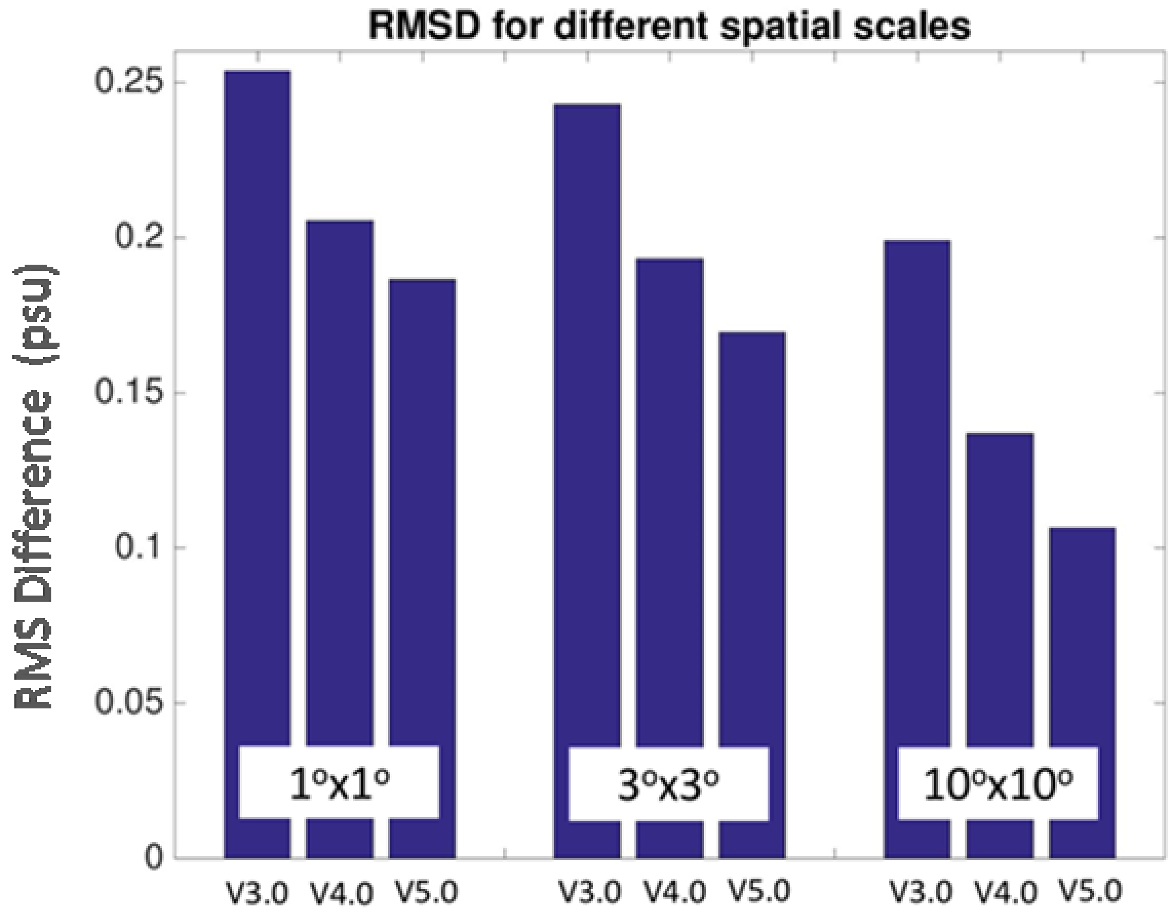
  24. Lee, T. Consistency of Aquarius sea surface salinity with Argo products on various spatial and temporal scales. Geophys. Res. Lett. 2016, 43, 3857–3864. [Google Scholar] [CrossRef]
  25. Klein, L.A.; Swift, C.T. An improved model for the dielectric constant of sea water at microwave frequencies. IEEE J. Ocean. Eng. 1977, AP-25, 104–111. [Google Scholar] [CrossRef]
  26. Meissner, T.; Wentz, F.J. The Emissivity of the Ocean Surface Between 6 and 90 GHz Over a Large Range of Wind Speeds and Earth Incidence Angles. IEEE Trans. Geosci. Remote Sens. 2012, 50, 3004–3026. [Google Scholar] [CrossRef]
  27. Zhou, Y.; Lang, R.H.; Dinnat, E.P.; Le Vine, D.M. L-Band Model Function of the Dielectric Constant of Seawater. IEEE Trans. Geosci. Remote Sens. 2017, 55, 6964–6974. [Google Scholar] [CrossRef]
  28. Wilson, W.J.; Yueh, S.H.; Dinardo, S.J.; Li, F.K. High-Stability L-Band Radiometer Measurements of Saltwater. IEEE Trans. Geosci. Remote Sens. 2004, 42, 1829–1835. [Google Scholar] [CrossRef]
  29. Dinnat, E.P.; Le Vine, D.M.; Piepmeier, J.R.; Brown, S.T.; Hong, L. Aquarius L-band Radiometers Calibration Using Cold Sky Observations. IEEE J. Sel. Top. Appl. Earth Obs. Remote Sens. 2015, 8, 5433–5449. [Google Scholar] [CrossRef]
  30. Scripps Institution of Oceanography. Global gridded NetCDF Argo only dataset produced by optimal interpolation. Available online: http://apdrc.soest.ucsd.edu/Gridded_fields.html (accessed on 1 October 2018).
  31. Piepmeier, J.R.; Hong, L.; Pellerano, F.A. Aquarius L-Band Microwave Radiometer: 3 Years of Radiometric Performance and Systematic Effects. IEEE J. Sel. Top. Appl. Earth Obs. Remote Sens. 2015, 8, 5416–5423. [Google Scholar] [CrossRef]
  32. Misra, S. Enabling the Next Generation of Salinity, Sea Surface Temperature and Wind Meaurements from Space: Instrument Challenges. In Proceedings of the Global Ocean Salinity and Water Cycle Workshop, Woods Hole, MA, USA, 22–26 May 2017. [Google Scholar]
  33. Dinnat, E.P.; Le Vine, D.M. Impact of sun glint on salinity remote sensing: An example with the aquarius radiometer. IEEE Trans. Geosci. Remote Sens. 2008, 46, 3137–3150. [Google Scholar] [CrossRef]
  34. Dinnat, E.P.; Boutin, J.; Yin, X.; Le Vine, D.; Waldteufel, P.; Vergely, J.-L. Comparison of SMOS and Aquarius sea surface salinity and analysis of possible causes for the differences. In Proceedings of the 2014 XXXIth URSI General Assembly and Scientific Symposium (URSI GASS), Beijing, China, 16–23 August 2014. [Google Scholar]
  35. Meissner, T.; Wentz, F.J. The complex dielectric constant of pure and sea water from microwave satellite observations. IEEE Trans. Geosci. Remote Sens. 2004, 42, 1836–1849. [Google Scholar] [CrossRef] [Green Version]
  36. Lang, R.; Zhou, Y.; Dinnat, E.; Le Vine, D. The Dielectric Constant Model Function and Implications for Remote Sensing of Salinity. In Proceedings of the IEEE International Geoscience and Remote Sensing Symposium (IGARSS), Fort Worth, TX, USA, 23–28 July 2017; pp. 3572–3574. [Google Scholar]
  37. Lang, R.; Zhou, Y.; Utku, C.; Le Vine, D. Accurate measurements of the dielectric constant of seawater at L band. Radio Sci. 2016, 51, 2–24. [Google Scholar] [CrossRef] [Green Version]
  38. Le Vine, D.M.; Lagerloef, G.S.E.; Torrusio, S.E. Aquarius and remote sensing of sea surface salinity from space. Proc. IEEE 2010, 98, 688–703. [Google Scholar] [CrossRef]
  39. Dinnat, E.P.; Le Vine, D.M.; Bindlish, R.; Piepmeier, J.R.; Brown, S.T. Aquarius whole range calibration: Celestial Sky, ocean, and land targets. In Proceedings of the 13th Specialist Meeting on Microwave Radiometry and Remote Sensing of the Environment (MicroRad), Pasadena, CA, USA, 24–27 March 2014; pp. 192–196. [Google Scholar]
  40. Le Vine, D.M.; Dinnat, E.P. Whole Range Calibration: Version 5.WR. AQ-014-PS-0030; 28 February 2018. Available online: https://podaac.jpl.nasa.gov/aquarius (accessed on 1 October 2018).
  41. Dinnat, E.P.; Le Vine, D.M.; Hong, L. Aquaruius Final Release Product and Full Range Calibration of L-Band Radiometer. In Proceedings of the IEEE International Geoscience and Remote Sensing Symposium (IGARSS2018), Valencia, Spain, 22–27 July 2018. [Google Scholar]
  42. Dinnat, E.; Le Vine, D.; Soldo, Y.; de Matthaeis, P. Theoretical algorithm for the retrieval of sea surface salinity from SMAP observations at L-band. In Proceedings of the 15th Specialist Meeting on Microwave Radiometry and Remote Sensing of the Environment, Cambridge, MA, USA, 27–30 March 2018. [Google Scholar]
  43. Meissner, T.; Wentz, F.; Ricciardulli, L.; Mears, C.; Manaster, A. Ocean Surface Salinity and Wind Speed from the SMAP L-Band Radiometer. In Microwave Radiometry and Remote Sensing of the Earth’s Surface and Atmosphere; VSP: Rancho Cordova, CA, USA, 2018. [Google Scholar]
  44. Meissner, T.; Wentz, F. Remote Sensing Systems SMAP Ocean Surface Salinities Level 2C, Version 2.0 Validated Release; Remote Sensing Systems: Santa Rosa, CA, USA, 2016. [Google Scholar]
  45. Sabia, R. SMOS Pilot-Mission Exploitation Platform (PI-MEP): A Hub for Validation and Expolitation of ESA SMOS Sea Surface Salinity Data. In Proceedings of the Ocean Sciences Meeting, Portland, OR, USA, 11–16 February 2018. [Google Scholar]
  46. Dong, X.; Shi, J.; Zhang, S.; Liu, H.; Wang, Z.; Zhu, D.; Zuo, L.; Chen, C.; Chen, W. Prelminary design of water cycle observation mission (WCOM). In Proceedings of the IEEE International Geoscience and Remote Sensing Symposium (IGARSS), Beijing, China, 10–15 July 2016; pp. 3434–3437. [Google Scholar]
  47. Shi, J.; Dong, X.; Zhao, T.; Du, Y.; Liu, H.; Wang, Z.; Zhu, D.; Ji, D.; Xiong, C.; Jiang, L. The Water Cycle Observation Mission (WCOM): Overview. In Proceedings of the IEEE International Geoscience and Remote Sensing Symposium (IGARSS), Beijing, China, 10–15 July 2016; pp. 3430–3433. [Google Scholar]
  48. Xu, X.; Yun, R.; Dong, X.; Zhu, D.; Yin, X.; Liu, H. Data Pre-Processing of MICAP (Microwave Imager Combined Active and Passive) Scatterometer. In Proceedings of the IEEE International Geoscience and Remote Sensing Symposium (IGARSS), Beijing, China, 10–15 July 2016; pp. 4776–4779. [Google Scholar]
  49. Dinnat, E.; de Amici, G.; Le Vine, D.; Piepmeier, J. Next generation spaceborne instrument for monitoring ocean salinity with application to the coastal zone and cryosphere. In Proceedings of the 15th Specialist Meeting on Microwave Radiometry and Remote Sensing of the Environment, Cambridge, MA, USA, 27–30 March 2018. [Google Scholar]
  50. Brown, S. A Next Generation Spaceborne Ocean State Observatory: Surface Salinity, Temperature and Ocean Winds from Equator to Pole. In Proceedings of the Globasl Ocean Salinity and the Water Cycle Workshop, Woods Hole, MA, USA, 22–26 May 2017. [Google Scholar]
Figure 1. The Aquarius/SAC-D observatory. Aquarius is the feed-reflector assembly to the left. SAC-D is the observatory bus to the right, plus several instruments.
Remotesensing 10 01585 g001
Figure 2. The root mean square (RMS) difference between Aquarius-retrieved sea surface salinity (SSS) and in situ ocean observations. The three bars in each group represent the three Aquarius beams. The groups are for different versions of the retrieval algorithm from Version 2 to the final Version 5. The data are from Figure 3 in Kao et al. [22].
Remotesensing 10 01585 g002
Figure 3. Aquarius SSS retrieval RMS error estimated with a triple point analysis using Aquarius, Hybrid Coordinate Ocean Model (HYCOM), and Argo data. The results shown are for the Aquarius middle beam. The dashed line represents the Aquarius mission requirement for monthly maps at 150-km spatial resolution. The data are from Table 1 in Kao et al. [22]. The version of HYCOM used by the Aquarius project is the HYCOM + NCODA Global 1/12° Analysis (GLBA0.08).
Remotesensing 10 01585 g003
Figure 4. Global average of regional temporal root mean square difference (RMSD) between Aquarius Level 3 monthly SSS and monthly Argo gridded maps as a function of the spatial scale for the entire mission. The three bars represent Version 3, 4, and 5 retrievals. The Argo data used in the comparison are from the gridded product from the Scripps Institute of Oceanography: http://apdrc.soest.ucsd.edu/Gridded_fields.html. The data are from Section 10 of Kao et al. [22], which also contains more detail.
Remotesensing 10 01585 g004
Figure 5. Flow diagram illustrating the steps in the Aquarius salinity retrieval algorithm. The process starts at the top with calibrated antenna temperature, TA, from the radiometer and ends with a measurement of SSS at the surface.
Remotesensing 10 01585 g005
Figure 6. The difference between observed and expected antenna temperature (TA bias) for beam 2 and horizontal polarization (a) before and (b) after removing an exponential fit for the temporal drift. Grey is the difference per orbit. Green (a) and red (b) are the average of the difference over a seven-day period (i.e., global average); red (a) is an exponential fit to the temporal drift (based on figures in Dinnat et al. [29]).
Remotesensing 10 01585 g006
Figure 7. Radiometer residual error, TA—TA_exp, after removing the exponential drift (a) and then correcting for the radiometer backend instability (bd). The data is for the Aquarius outer beam and horizontal polarization. Grey is the difference per orbit, and green is a seven-day average. Red in (c,d) shows the residual when looking at cold sky superimposed on the data in (b) (with a shift of 0.05 to align the curves). Crosses “+” indicate the data points. Blue in (d) shows the temperature of correlated noise diode centered on zero.
Remotesensing 10 01585 g007
Figure 8. Salinity error (difference between retrieved SSS and in situ salinity from Argo) as a function of sea surface temperature, SST. Grey are the data and red is the median value. (Author’s figure from Le Vine et al. [4]).
Remotesensing 10 01585 g008
Figure 9. Salinity error as a function of sea surface temperature, SST, when using three different model functions for the dielectric constant of sea water in the retrieval. The three model functions are: Klein–Swift [25], Meissner–Wentz [26], and George Washington University [36]. (Author’s figure from Zhou et al. [36]).
Remotesensing 10 01585 g009
Figure 10. Aquarius measured antenna temperature, Ta_measured, plotted against the antenna temperature predicted with the forward model, Ta_model, for three regimes: cold sky (magenta insert), ocean (blue insert), and land (Little River watershed, red dots). The data is for horizontal polarization, and the middle beam and the measurements are from V2.0 of the algorithm. (Author’s figure from Le Vine et al. [4]).
Remotesensing 10 01585 g010
Figure 11. Aquarius measured antenna temperature, Ta_measured, plotted against the antenna temperature predicted with the forward model, Ta_model, for three regimes: cold sky (magenta insert), ocean (blue insert), and Little Washita watershed (red dots). The data are for the outer Aquarius beam and horizontal polarizations, and Version 5.WR, the final release of the algorithm with the full range calibration. Insets are close-ups of ocean and Sky data.
Remotesensing 10 01585 g011
Figure 12. Salinity from the Soil Moisture Active Passive (SMAP) satellite: (a) global maps of SSS, remote sensing systems, Version 2, two-year average, 2015–2016; (b) salinity error, difference between retrieved SSS and in situ from Argo.
Remotesensing 10 01585 g012aRemotesensing 10 01585 g012b
Table 1. Values for the coefficients (a, b).
V-PolH-Pol
a b a b
Beam 11.003350568406014−3.5928572808254681.007405352181248−6.595668007611077
Beam 21.008337848581688−9.6556108625975331.003498234086013−2.948722716952730
Beam 31.017695610594212−2.2339116095233801.001311195384693−1.075651639210478

