Landslide Detection and Susceptibility Mapping by AIRSAR Data Using Support Vector Machine and Index of Entropy Models in Cameron Highlands, Malaysia

 ,
,  , ,
, ,  ,
, 
 ,
,  and
and
Abstract
1. Introduction
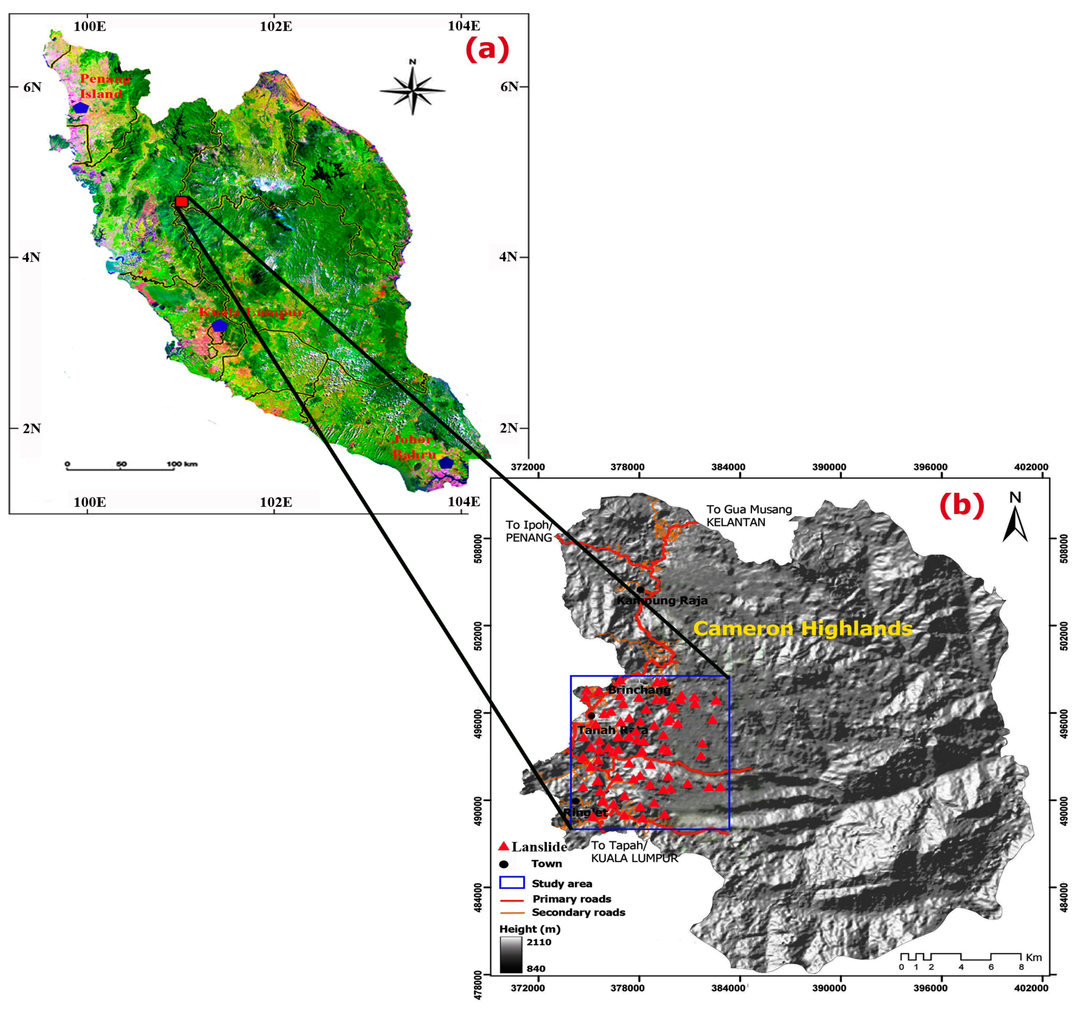
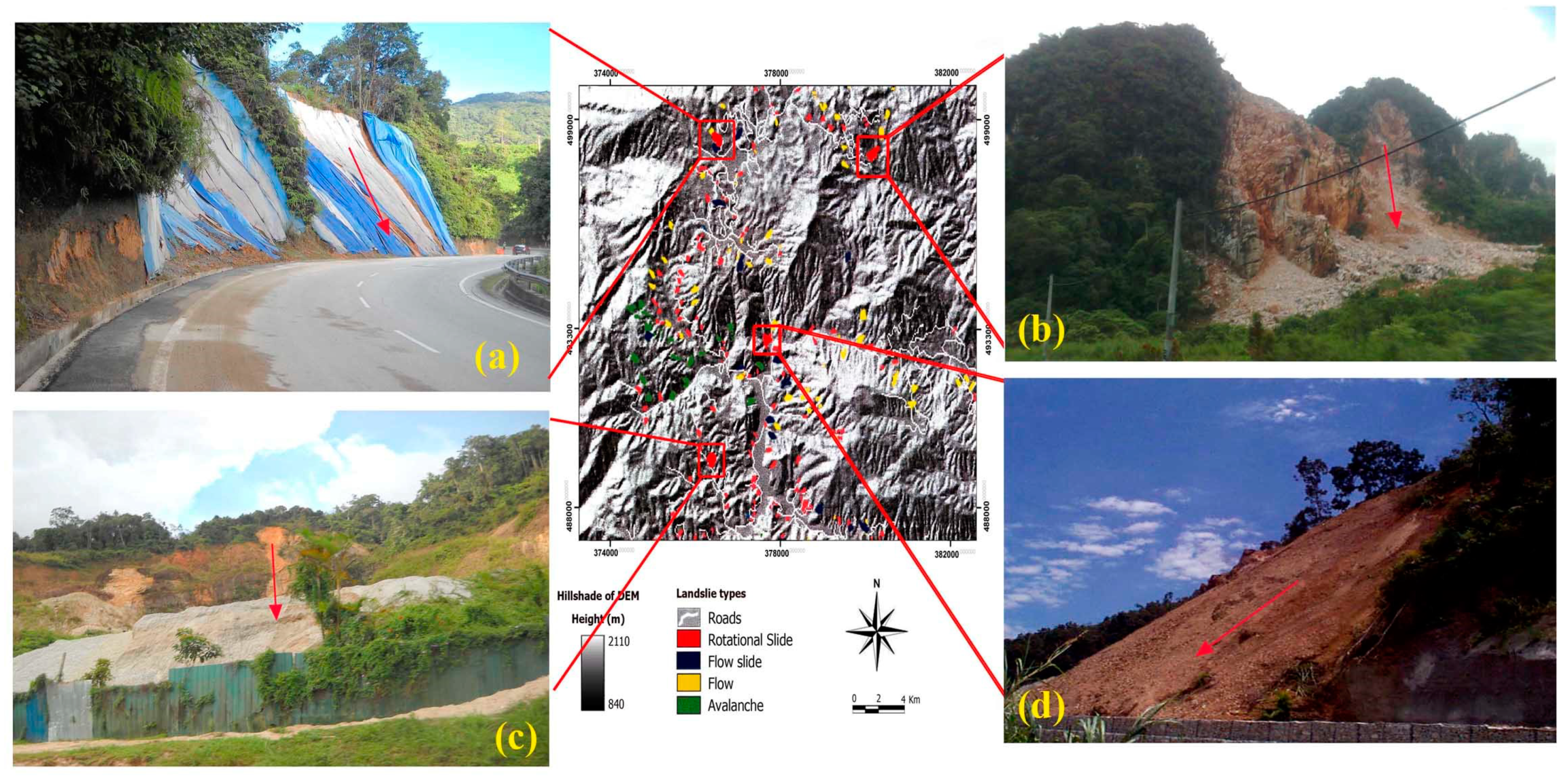
2. Description of the Study Area
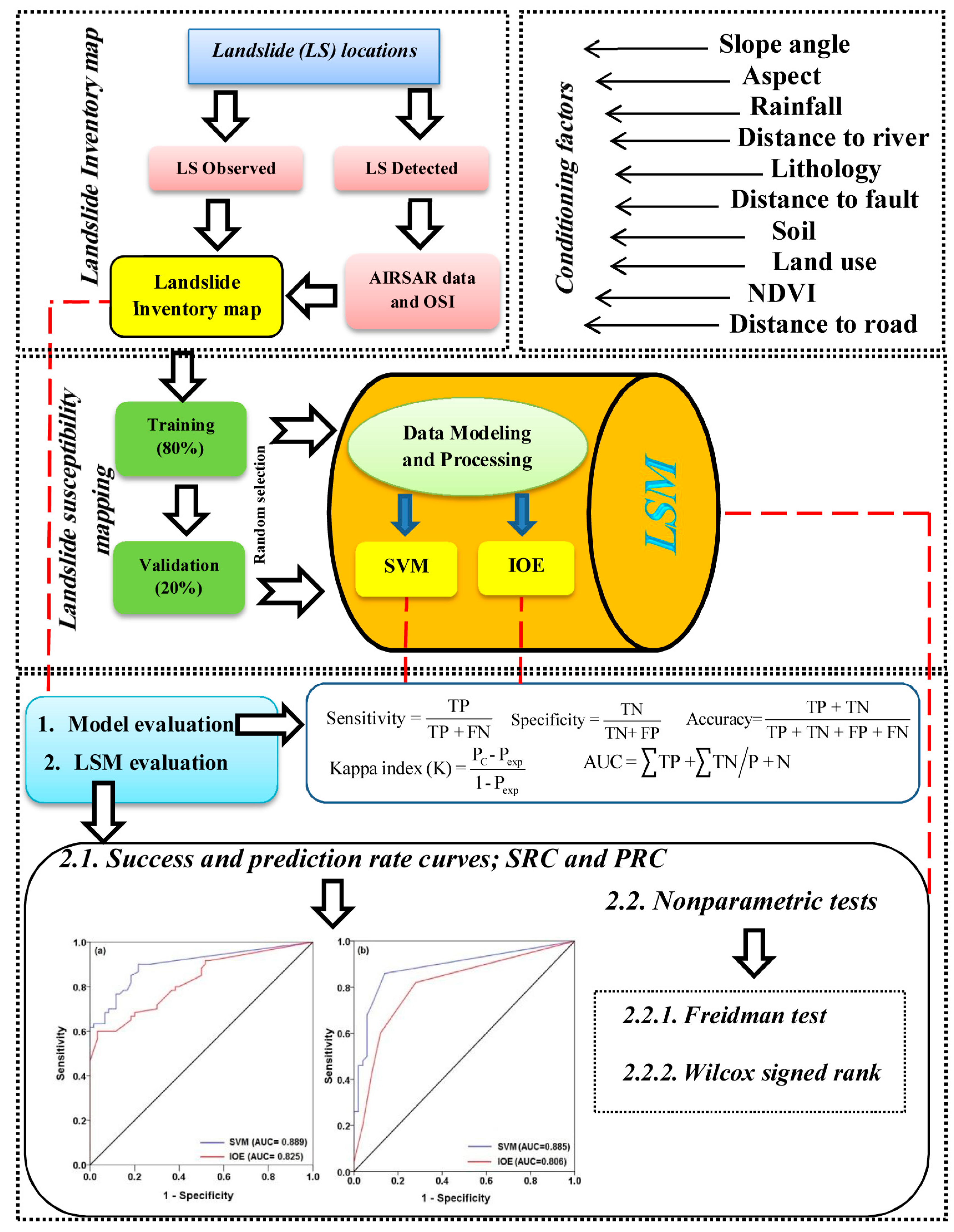
3. Materials and Methods
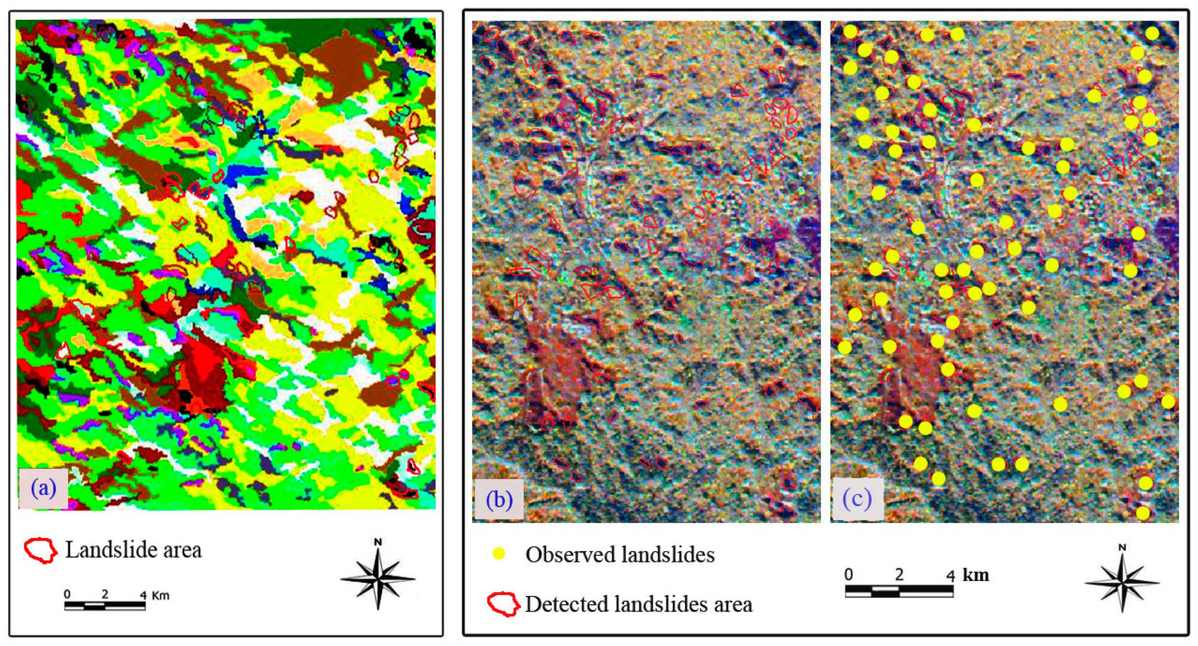
3.1. Landslide Inventory Map
3.2. Landslide Geodatabase
Landslide Conditioning Factors
3.3. Landslide Susceptibility Models
3.3.1. Support Vector Machine
3.3.2. Index of Entropy
3.4. Model Validation and Comparison
3.4.1. Statistical-Based Measures
3.4.2. ROC Curve Analysis
3.5. Statistical Tests (Friedman and Wilcoxon)
4. Results and Analysis
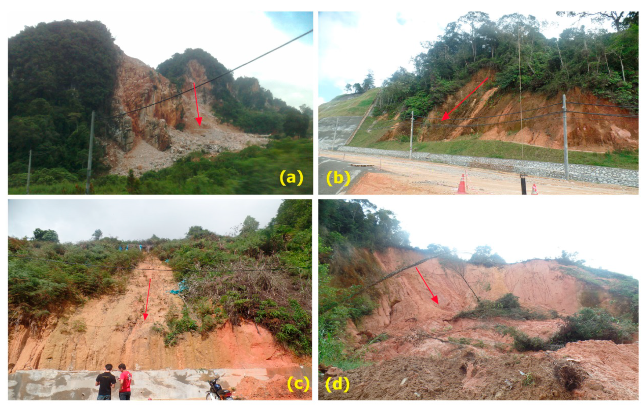
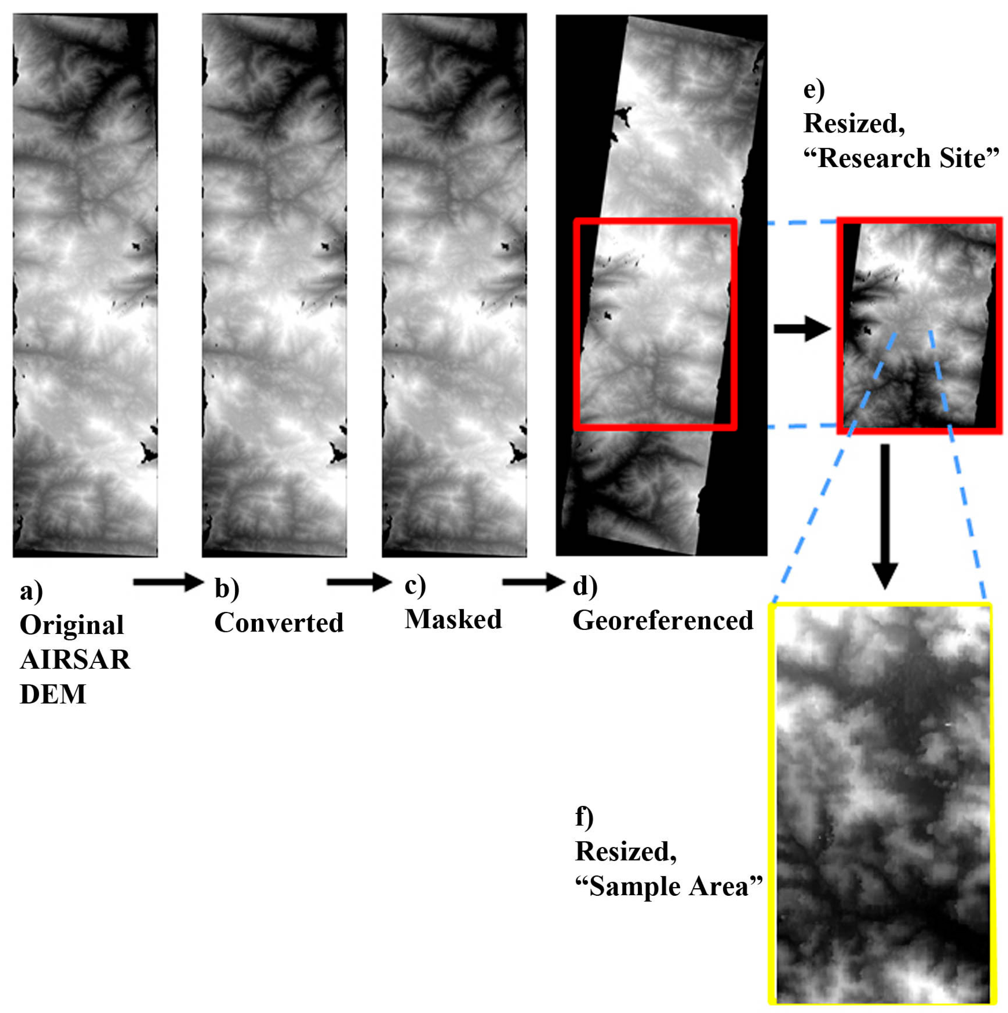
4.1. Landslide Detection Using AIRSAR and Optical Satellite Images
4.2. Model Analysis and Results
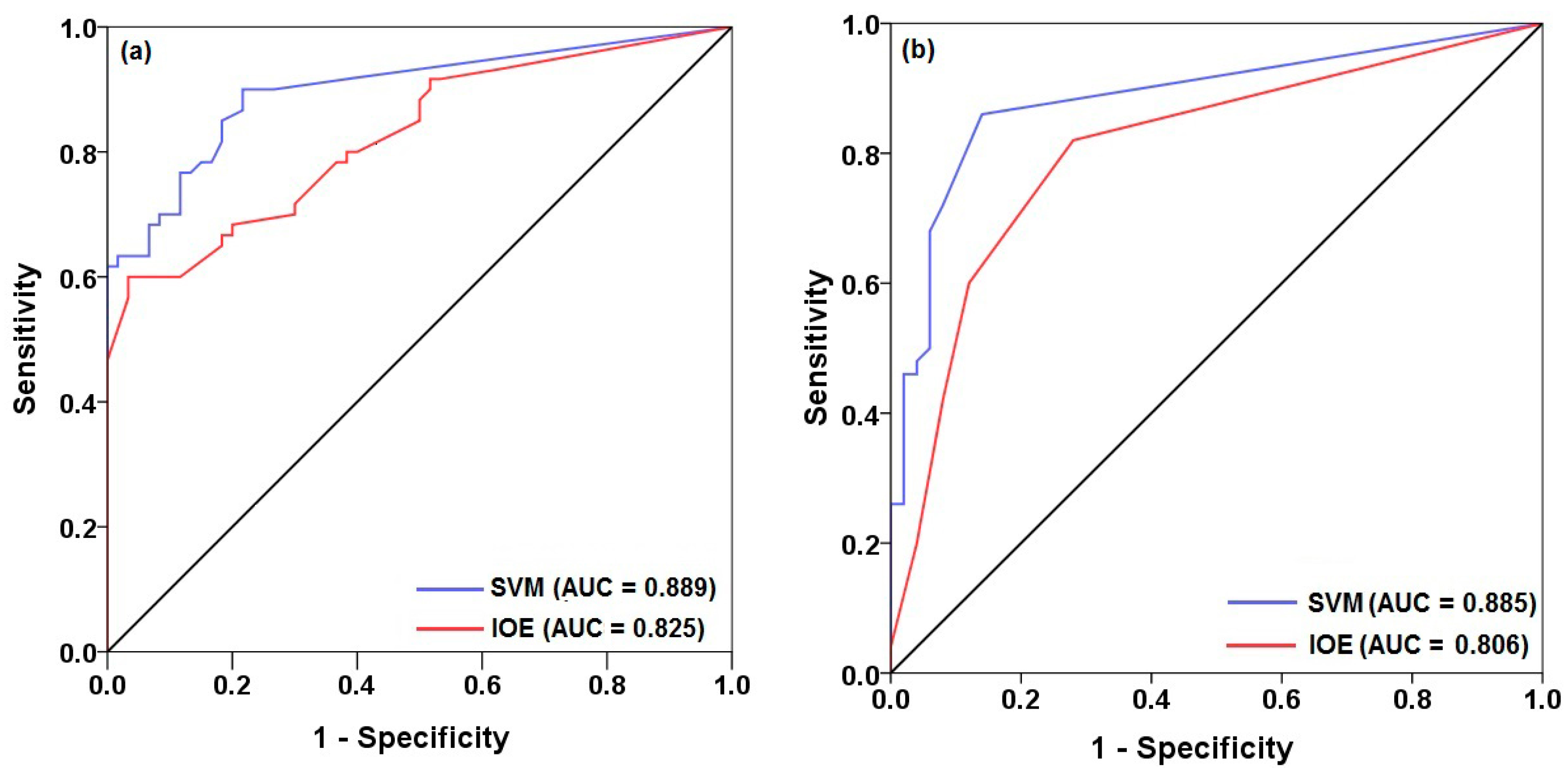
4.3. Model Validation and Comparison
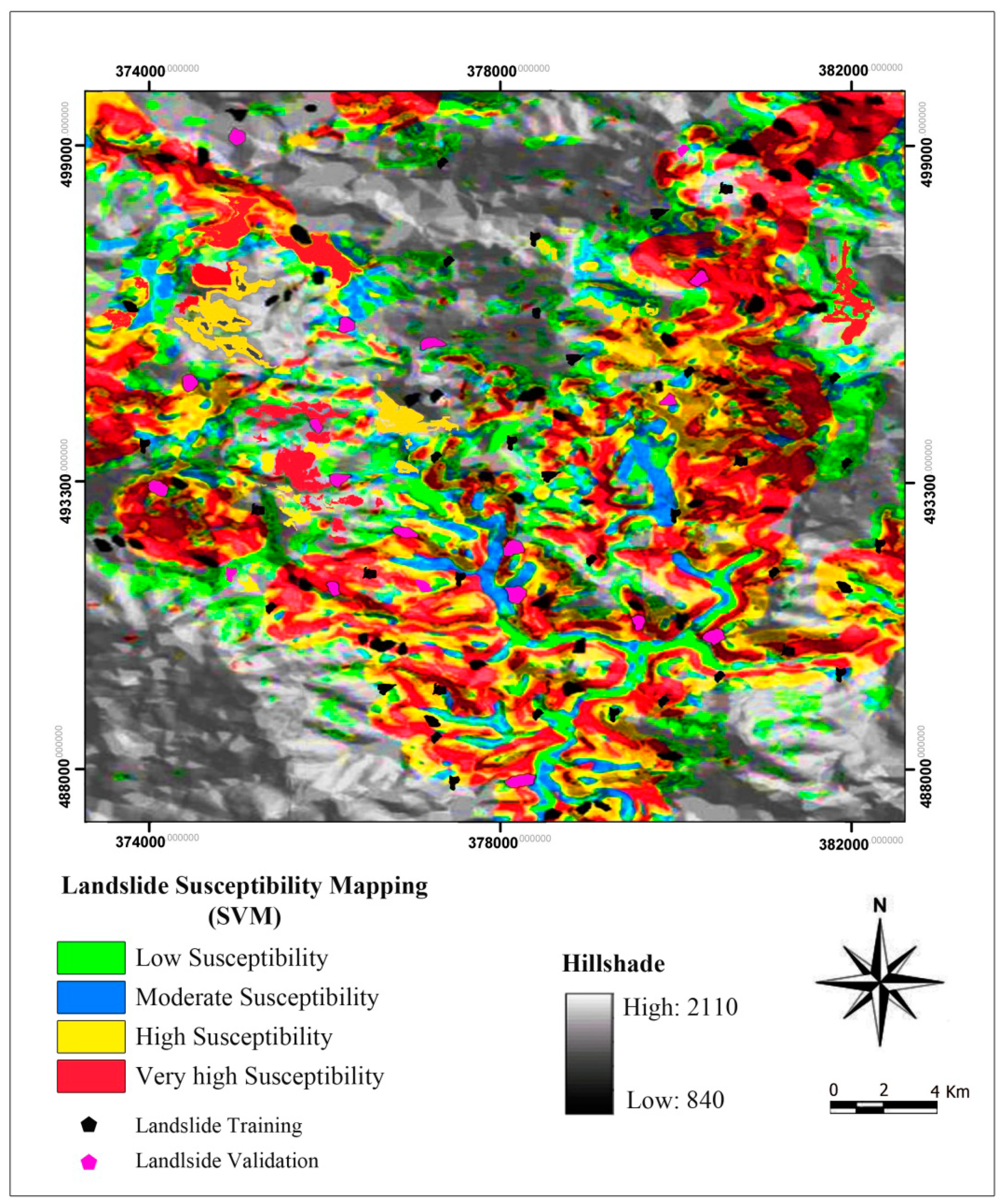
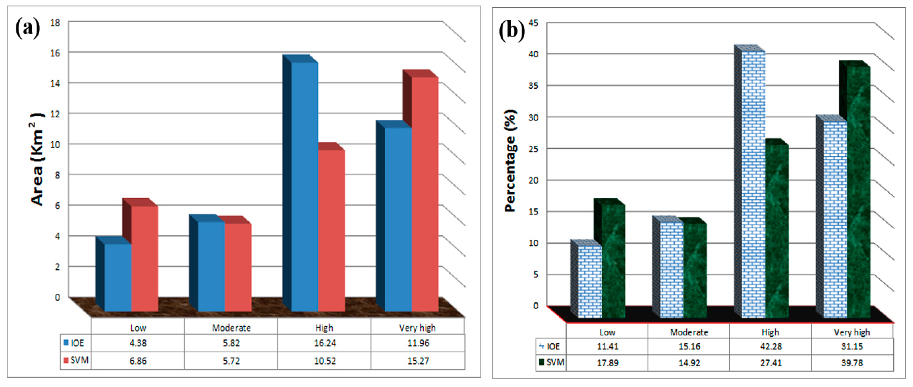
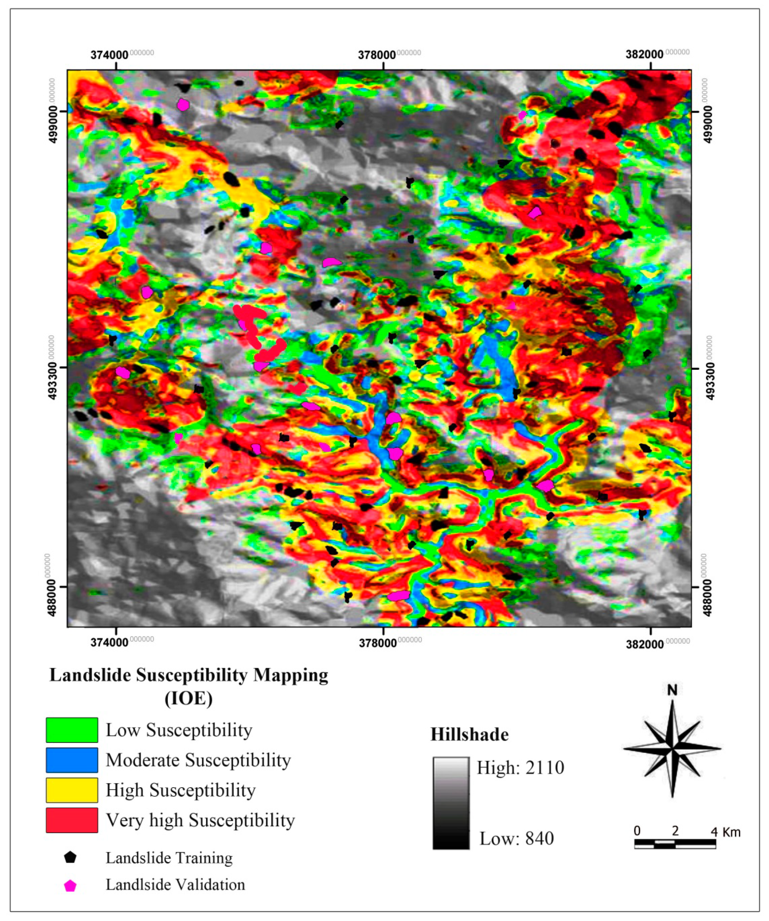
4.4. Generating Landslide Susceptibility Mapping and Comparison
4.4.1. LSM by SVM Model
4.4.2. LSM by the IOE Model
5. Discussion
6. Conclusions
Author Contributions
Funding
Acknowledgments
Conflicts of Interest
References
- Yilmaz, I. Comparison of landslide susceptibility mapping methodologies for Koyulhisar, Turkey: Conditional probability, logistic regression, artificial neural networks, and support vector machine. Environ. Earth Sci. 2010, 61, 821–836. [Google Scholar] [CrossRef]
- Pourghasemi, H.R.; Mohammady, M.; Pradhan, B. Landslide susceptibility mapping using index of entropy and conditional probability models in GIS: Safarood basin, Iran. Catena 2012, 97, 71–84. [Google Scholar] [CrossRef]
- Takara, K.; Yamashiki, Y.; Sassa, K.; Ibrahim, A.B.; Fukuoka, H. A distributed hydrological–geotechnical model using satellite-derived rainfall estimates for shallow landslide prediction system at a catchment scale. Landslides 2010, 7, 237–258. [Google Scholar]
- Pradhan, B.; Sezer, E.A.; Gokceoglu, C.; Buchroithner, M.F. Landslide susceptibility mapping by neuro-fuzzy approach in a landslide-prone area (cameron highlands, Malaysia). IEEE Trans. Geosci. Remote Sens. 2010, 48, 4164–4177. [Google Scholar] [CrossRef]
- Pradhan, B. Landslide susceptibility mapping of a catchment area using frequency ratio, fuzzy logic and multivariate logistic regression approaches. J. Indian Soc. Remote Sens. 2010, 38, 301–320. [Google Scholar] [CrossRef]
- Shahabi, H.; Ahmad, B.; Khezri, S. Evaluation and comparison of bivariate and multivariate statistical methods for landslide susceptibility mapping (case study: Zab basin). Arab. J. Geosci. 2013, 6, 3885–3907. [Google Scholar] [CrossRef]
- Dai, F.; Lee, C.; Ngai, Y.Y. Landslide risk assessment and management: An overview. Eng. Geol. 2002, 64, 65–87. [Google Scholar] [CrossRef]
- Razak, K.A.; Santangelo, M.; Van Westen, C.J.; Straatsma, M.W.; de Jong, S.M. Generating an optimal dtm from airborne laser scanning data for landslide mapping in a tropical forest environment. Geomorphology 2013, 190, 112–125. [Google Scholar] [CrossRef]
- Corominas, J.; Van Westen, C.; Frattini, P.; Cascini, L.; Malet, J.-P.; Fotopoulou, S.; Catani, F.; Van Den Eeckhaut, M.; Mavrouli, O.; Agliardi, F. Recommendations for the quantitative analysis of landslide risk. Bull. Eng. Geol. Environ. 2014, 73, 209–263. [Google Scholar] [CrossRef]
- Ouchi, K. Recent trend and advance of synthetic aperture radar with selected topics. Remote Sens. 2013, 5, 716–807. [Google Scholar] [CrossRef]
- Joyce, K.E.; Belliss, S.E.; Samsonov, S.V.; McNeill, S.J.; Glassey, P.J. A review of the status of satellite remote sensing and image processing techniques for mapping natural hazards and disasters. Prog. Phys. Geogr. 2009, 33, 183–207. [Google Scholar] [CrossRef]
- Teshebaeva, K.; Roessner, S.; Echtler, H.; Motagh, M.; Wetzel, H.-U.; Molodbekov, B. Alos/palsar insar time-series analysis for detecting very slow-moving landslides in southern Kyrgyzstan. Remote Sens. 2015, 7, 8973–8994. [Google Scholar] [CrossRef]
- Corsini, A.; Farina, P.; Antonello, G.; Barbieri, M.; Casagli, N.; Coren, F.; Guerri, L.; Ronchetti, F.; Sterzai, P.; Tarchi, D. Space-borne and ground-based sar interferometry as tools for landslide hazard management in civil protection. Int. J. Remote Sens. 2006, 27, 2351–2369. [Google Scholar] [CrossRef]
- Du, Y.; Xu, Q.; Zhang, L.; Feng, G.; Li, Z.; Chen, R.-F.; Lin, C.-W. Recent landslide movement in tsaoling, taiwan tracked by terrasar-x/tandem-x dem time series. Remote Sens. 2017, 9, 353. [Google Scholar] [CrossRef]
- Plank, S.; Twele, A.; Martinis, S. Landslide mapping in vegetated areas using change detection based on optical and polarimetric sar data. Remote Sens. 2016, 8, 307. [Google Scholar] [CrossRef]
- Raspini, F.; Ciampalini, A.; Del Conte, S.; Lombardi, L.; Nocentini, M.; Gigli, G.; Ferretti, A.; Casagli, N. Exploitation of amplitude and phase of satellite sar images for landslide mapping: The case of montescaglioso (South Italy). Remote Sens. 2015, 7, 14576–14596. [Google Scholar] [CrossRef]
- Shi, X.; Liao, M.; Li, M.; Zhang, L.; Cunningham, C. Wide-area landslide deformation mapping with multi-path alos palsar data stacks: A case study of three gorges area, China. Remote Sens. 2016, 8, 136. [Google Scholar] [CrossRef]
- Kawabata, D.; Bandibas, J. Landslide susceptibility mapping using geological data, a dem from aster images and an artificial neural network (ANN). Geomorphology 2009, 113, 97–109. [Google Scholar] [CrossRef]
- Oh, H.-J.; Park, N.-W.; Lee, S.-S.; Lee, S. Extraction of landslide-related factors from aster imagery and its application to landslide susceptibility mapping. Int. J. Remote Sens. 2012, 33, 3211–3231. [Google Scholar] [CrossRef]
- Zhao, C.; Zhong, L. Remote Sensing of Landslides—A Review. Remote. Sens. 2018, 10, 279. [Google Scholar] [CrossRef]
- Stumpf, A.; Michéa, D.; Malet, J.P. Improved Co-Registration of Sentinel-2 and Landsat-8 Imagery for Earth Surface Motion Measurements. Remote Sens. 2018, 10, 160. [Google Scholar] [CrossRef]
- Ercanoglu, M.; Gokceoglu, C.; Van Asch, T.W. Landslide susceptibility zoning north of yenice (NW Turkey) by multivariate statistical techniques. Nat. Hazards 2004, 32, 1–23. [Google Scholar] [CrossRef]
- Gupta, R.; Joshi, B. Landslide hazard zoning using the gis approach—A case study from the ramganga catchment, himalayas. Eng. Geol. 1990, 28, 119–131. [Google Scholar] [CrossRef]
- Van Westen, C. GIS in landslide hazard zonation: A review, with examples from the andes of colombia. In Mountain Environment Regional Information Systems; Taylor & Francis: London, UK, 1994; pp. 135–166. ISBN 0-7484-0088-5. [Google Scholar]
- Nagarajan, R.; Mukherjee, A.; Roy, A.; Khire, M. Technical note temporal remote sensing data and GIS application in landslide hazard zonation of part of western ghat, India. Int. J. Remote Sens. 1998, 19, 573–585. [Google Scholar] [CrossRef]
- Constantin, M.; Bednarik, M.; Jurchescu, M.C.; Vlaicu, M. Landslide susceptibility assessment using the bivariate statistical analysis and the index of entropy in the Sibiciu basin (Romania). Environ. Earth Sci. 2011, 63, 397–406. [Google Scholar] [CrossRef]
- Blahut, J.; Klimeš, J.; Vařilová, Z. Quantitative rockfall hazard and risk analysis in selected municipalities of the české švýcarsko national park, northwestern Czechia. Geografie 2013, 118, 205–220. [Google Scholar]
- Ciabatta, L.; Brocca, L.; Massari, C.; Moramarco, T.; Puca, S.; Rinollo, A.; Gabellani, S.; Wagner, W. Integration of satellite soil moisture and rainfall observations over the Italian territory. J. Hydrometeorol. 2015, 16, 1341–1355. [Google Scholar] [CrossRef]
- Oliveira, S.; Zêzere, J.; Catalão, J.; Nico, G. The contribution of psinsar interferometry to landslide hazard in weak rock-dominated areas. Landslides 2015, 12, 703–719. [Google Scholar] [CrossRef]
- Shahabi, H.; Hashim, M. Landslide susceptibility mapping using GIS-based statistical models and remote sensing data in tropical environment. Sci. Rep. 2015, 5, 9899. [Google Scholar] [CrossRef] [PubMed]
- Tan, Y.; Guo, D.; Xu, B. A geospatial information quantity model for regional landslide risk assessment. Nat. Hazards 2015, 79, 1385–1398. [Google Scholar] [CrossRef]
- Jebur, M.N.; Pradhan, B.; Tehrany, M.S. Using alos palsar derived high-resolution dinsar to detect slow-moving landslides in tropical forest: Cameron highlands, malaysia. Geomat. Nat. Hazards Risk 2015, 6, 741–759. [Google Scholar] [CrossRef]
- Vahidnia, M.H.; Alesheikh, A.A.; Alimohammadi, A.; Hosseinali, F. A GIS-based neuro-fuzzy procedure for integrating knowledge and data in landslide susceptibility mapping. Comput. Geosci. 2010, 36, 1101–1114. [Google Scholar] [CrossRef]
- Yalcin, A. GIS-based landslide susceptibility mapping using analytical hierarchy process and bivariate statistics in ardesen (Turkey): Comparisons of results and confirmations. Catena 2008, 72, 1–12. [Google Scholar] [CrossRef]
- Mondal, S.; Maiti, R. Landslide susceptibility analysis of Shiv-khola watershed, Darjiling: A Remote sensing & GIS based analytical hierarchy process (AHP). J. Indian Soc. Remote Sens. 2012, 40, 483–496. [Google Scholar]
- Kayastha, P.; Dhital, M.; De Smedt, F. Application of the analytical hierarchy process (AHP) for landslide susceptibility mapping: A case study from the Tinau Watershed, west Nepal. Comput. Geosci. 2013, 52, 398–408. [Google Scholar] [CrossRef]
- Shahabi, H.; Khezri, S.; Ahmad, B.B.; Hashim, M. Landslide susceptibility mapping at central Zab basin, Iran: A comparison between analytical hierarchy process, frequency ratio and logistic regression models. Catena 2014, 115, 55–70. [Google Scholar] [CrossRef]
- Nefeslioglu, H.; Gokceoglu, C.; Sonmez, H. An assessment on the use of logistic regression and artificial neural networks with different sampling strategies for the preparation of landslide susceptibility maps. Eng. Geol. 2008, 97, 171–191. [Google Scholar] [CrossRef]
- Yilmaz, I. Landslide susceptibility mapping using frequency ratio, logistic regression, artificial neural networks and their comparison: A case study from Kat Landslides (Tokat—Turkey). Comput. Geosci. 2009, 35, 1125–1138. [Google Scholar] [CrossRef]
- Pradhan, B.; Lee, S. Regional landslide susceptibility analysis using back-propagation neural network model at Cameron Highland, Malaysia. Landslides 2010, 7, 13–30. [Google Scholar] [CrossRef]
- Akgun, A.; Kıncal, C.; Pradhan, B. Application of remote sensing data and gis for landslide risk assessment as an environmental threat to Izmir city (West Turkey). Environ. Monit. Assess. 2012, 184, 5453–5470. [Google Scholar] [CrossRef] [PubMed]
- Wang, L.-J.; Sawada, K.; Moriguchi, S. Landslide susceptibility analysis with logistic regression model based on fcm sampling strategy. Comput. Geosci. 2013, 57, 81–92. [Google Scholar] [CrossRef]
- Regmi, A.D.; Yoshida, K.; Pourghasemi, H.R.; DhitaL, M.R.; Pradhan, B. Landslide susceptibility mapping along Bhalubang—Shiwapur area of mid-western Nepal using frequency ratio and conditional probability models. J. Mt. Sci. 2014, 11, 1266–1285. [Google Scholar] [CrossRef]
- Shahabi, H.; Hashim, M.; Ahmad, B.B. Remote sensing and GIS-based landslide susceptibility mapping using frequency ratio, logistic regression, and fuzzy logic methods at the central Zab basin, Iran. Environ. Earth Sci. 2015, 73, 8647–8668. [Google Scholar] [CrossRef]
- Parise, M.; Jibson, R.W. A seismic landslide susceptibility rating of geologic units based on analysis of characteristics of landslides triggered by the 17 January, 1994 northridge, california earthquake. Eng. Geol. 2000, 58, 251–270. [Google Scholar] [CrossRef]
- Jibson, R.W.; Harp, E.L.; Michael, J.A. A method for producing digital probabilistic seismic landslide hazard maps. Eng. Geol. 2000, 58, 271–289. [Google Scholar] [CrossRef]
- Cevik, E.; Topal, T. GIS-based landslide susceptibility mapping for a problematic segment of the natural gas pipeline, Hendek (Turkey). Environ. Geol. 2003, 44, 949–962. [Google Scholar] [CrossRef]
- Akgün, A.; Bulut, F. GIS-based landslide susceptibility for arsin-yomra (Trabzon, North Turkey) region. Environ. Geol. 2007, 51, 1377–1387. [Google Scholar] [CrossRef]
- Dahal, R.K.; Hasegawa, S.; Nonomura, A.; Yamanaka, M.; Masuda, T.; Nishino, K. GIS-based weights-of-evidence modeling of rainfall-induced landslides in small catchments for landslide susceptibility mapping. Environ. Geol. 2008, 54, 311–324. [Google Scholar] [CrossRef]
- Remondo, J.; González, A.; De Terán, J.R.D.; Cendrero, A.; Fabbri, A.; Chung, C.-J.F. Validation of landslide susceptibility maps; examples and applications from a case study in Northern Spain. Nat. Hazards 2003, 30, 437–449. [Google Scholar] [CrossRef]
- Devkota, K.C.; Regmi, A.D.; Pourghasemi, H.R.; Yoshida, K.; Pradhan, B.; Ryu, I.C.; Dhital, M.R.; Althuwaynee, O.F. Landslide susceptibility mapping using certainty factor, index of entropy and logistic regression models in GIS and their comparison at mugling–narayanghat road section in Nepal Himalaya. Nat. Hazards 2013, 65, 135–165. [Google Scholar] [CrossRef]
- Pourghasemi, H.R.; Pradhan, B.; Gokceoglu, C.; Mohammadi, M.; Moradi, H.R. Application of weights-of-evidence and certainty factor models and their comparison in landslide susceptibility mapping at Haraz watershed, Iran. Arab. J. Geosci. 2013, 6, 2351–2365. [Google Scholar] [CrossRef]
- Binaghi, E.; Luzi, L.; Madella, P.; Pergalani, F.; Rampini, A. Slope instability zonation: A comparison between certainty factor and fuzzy Dempster–Shafer approaches. Nat. Hazards 1998, 17, 77–97. [Google Scholar] [CrossRef]
- Ozdemir, A.; Altural, T. A comparative study of frequency ratio, weights of evidence and logistic regression methods for landslide susceptibility mapping: Sultan mountains, SW Turkey. J. Asian Earth Sci. 2013, 64, 180–197. [Google Scholar] [CrossRef]
- Regmi, A.D.; Devkota, K.C.; Yoshida, K.; Pradhan, B.; Pourghasemi, H.R.; Kumamoto, T.; Akgun, A. Application of frequency ratio, statistical index, and weights-of-evidence models and their comparison in landslide susceptibility mapping in central Nepal himalaya. Arab. J. Geosci. 2014, 7, 725–742. [Google Scholar] [CrossRef]
- Althuwaynee, O.F.; Pradhan, B.; Park, H.-J.; Lee, J.H. A novel ensemble bivariate statistical evidential belief function with knowledge-based analytical hierarchy process and multivariate statistical logistic regression for landslide susceptibility mapping. Catena 2014, 114, 21–36. [Google Scholar] [CrossRef]
- Tien Bui, D.; Pradhan, B.; Revhaug, I.; Nguyen, D.B.; Pham, H.V.; Bui, Q.N. A novel hybrid evidential belief function-based fuzzy logic model in spatial prediction of rainfall-induced shallow landslides in the Lang Son city area (Vietnam). Geomat. Nat. Hazards Risk 2015, 6, 243–271. [Google Scholar]
- Chen, W.; Pourghasemi, H.R.; Zhao, Z. A GIS-based comparative study of dempster-shafer, logistic regression and artificial neural network models for landslide susceptibility mapping. Geocarto Int. 2017, 32, 367–385. [Google Scholar] [CrossRef]
- Tien Bui, D.; Pradhan, B.; Lofman, O.; Revhaug, I.; Dick, O.B. Spatial prediction of landslide hazards in HOA Binh province (Vietnam): A comparative assessment of the efficacy of evidential belief functions and fuzzy logic models. Catena 2012, 96, 28–40. [Google Scholar] [CrossRef]
- Dou, J.; Yamagishi, H.; Pourghasemi, H.R.; Yunus, A.P.; Song, X.; Xu, Y.; Zhu, Z. An integrated artificial neural network model for the landslide susceptibility assessment of Osado Island, Japan. Nat. Hazards 2015, 78, 1749–1776. [Google Scholar] [CrossRef]
- Polykretis, C.; Ferentinou, M.; Chalkias, C. A comparative study of landslide susceptibility mapping using landslide susceptibility index and artificial neural networks in the Krios River and Krathis River catchments (Northern Peloponnesus, Greece). Bull. Eng. Geol. Environ. 2015, 74, 27–45. [Google Scholar] [CrossRef]
- Tien Bui, D.; Tuan, T.A.; Klempe, H.; Pradhan, B.; Revhaug, I. Spatial prediction models for shallow landslide hazards: A comparative assessment of the efficacy of support vector machines, artificial neural networks, kernel logistic regression, and logistic model tree. Landslides 2016, 13, 361–378. [Google Scholar] [CrossRef]
- Chen, W.; Pourghasemi, H.R.; Naghibi, S.A. Prioritization of landslide conditioning factors and its spatial modeling in Shangnan county, China using GIS-based data mining algorithms. Bull. Eng. Geol. Environ. 2018, 77, 611–629. [Google Scholar] [CrossRef]
- Chen, W.; Xie, X.; Wang, J.; Pradhan, B.; Hong, H.; Bui, D.T.; Duan, Z.; Ma, J. A comparative study of logistic model tree, random forest, and classification and regression tree models for spatial prediction of landslide susceptibility. CATENA 2017, 151, 147–160. [Google Scholar] [CrossRef]
- Chen, W.; Peng, J.; Hong, H.; Shahabi, H.; Pradhan, B.; Liu, J.; Zhu, A.X.; Pei, X.; Duan, Z. Landslide susceptibility modeling using GIS-based machine learning techniques for Chongren County, Jiangxi Province, China. Sci. Total Environ. 2018, 626, 1121–1135. [Google Scholar] [CrossRef] [PubMed]
- Trigila, A.; Iadanza, C.; Esposito, C.; Scarascia-Mugnozza, G. Comparison of logistic regression and random forests techniques for shallow landslide susceptibility assessment in Giampilieri (NE Sicily, Italy). Geomorphology 2015, 249, 119–136. [Google Scholar] [CrossRef]
- Chen, W.; Xie, X.; Peng, J.; Wang, J.; Duan, Z.; Hong, H. Gis-based landslide susceptibility modeling: A comparative assessment of kernel logistic regression, naïve-bayes tree, and alternating decision tree models. Geomat. Nat. Hazards Risk 2017, 8, 950–973. [Google Scholar] [CrossRef]
- Hong, H.; Pradhan, B.; Xu, C.; Bui, D.T. Spatial prediction of landslide hazard at the Yihuang area (China) using two-class kernel logistic regression, alternating decision tree and support vector machines. Catena 2015, 133, 266–281. [Google Scholar] [CrossRef]
- Pradhan, B. A comparative study on the predictive ability of the decision tree, support vector machine and neuro-fuzzy models in landslide susceptibility mapping using GIS. Comput. Geosci. 2013, 51, 350–365. [Google Scholar] [CrossRef]
- Chen, W.; Wang, J.; Xie, X.; Hong, H.; Trung, N.V.; Bui, D.T.; Wang, G.; Li, X. Spatial prediction of landslide susceptibility using integrated frequency ratio with entropy and support vector machines by different kernel functions. Environ. Earth Sci. 2016, 75, 1344. [Google Scholar] [CrossRef]
- Hong, H.; Pradhan, B.; Jebur, M.N.; Bui, D.T.; Xu, C.; Akgun, A. Spatial prediction of landslide hazard at the Luxi area (China) using support vector machines. Environ. Earth Sci. 2016, 75, 1–14. [Google Scholar] [CrossRef]
- Tien Bui, D.; Pham, B.T.; Nguyen, Q.P.; Hoang, N.-D. Spatial prediction of rainfall-induced shallow landslides using hybrid integration approach of least-squares support vector machines and differential evolution optimization: A case study in central Vietnam. Int. J. Digit. Earth 2016, 9, 1077–1097. [Google Scholar] [CrossRef]
- Chen, W.; Pourghasemi, H.R.; Naghibi, S.A. A comparative study of landslide susceptibility maps produced using support vector machine with different kernel functions and entropy data mining models in China. Bull. Eng. Geol. Environ. 2017, 77, 647–664. [Google Scholar] [CrossRef]
- Tien Bui, D.; Pradhan, B.; Lofman, O.; Revhaug, I. Landslide susceptibility assessment in Vietnam using support vector machines, decision tree, and naive bayes models. Math. Probl. Eng. 2012, 2012, 974638. [Google Scholar] [CrossRef]
- Dehnavi, A.; Aghdam, I.N.; Pradhan, B.; Varzandeh, M.H.M. A new hybrid model using step-wise weight assessment ratio analysis (SWARA) technique and adaptive neuro-fuzzy inference system (ANFIS) for regional landslide hazard assessment in Iran. Catena 2015, 135, 122–148. [Google Scholar] [CrossRef]
- Aghdam, I.N.; Varzandeh, M.H.M.; Pradhan, B. Landslide susceptibility mapping using an ensemble statistical index (WI) and adaptive neuro-fuzzy inference system (ANFIS) model at Alborz mountains (Iran). Environ. Earth Sci. 2016, 75, 1–20. [Google Scholar] [CrossRef]
- Lee, S.; Ryu, J.-H.; Won, J.-S.; Park, H.-J. Determination and application of the weights for landslide susceptibility mapping using an artificial neural network. Eng. Geol. 2004, 71, 289–302. [Google Scholar] [CrossRef]
- He, S.; Pan, P.; Dai, L.; Wang, H.; Liu, J. Application of kernel-based fisher discriminant analysis to map landslide susceptibility in the Qinggan river delta, three Gorges, China. Geomorphology 2012, 171, 30–41. [Google Scholar] [CrossRef]
- Peng, L.; Niu, R.; Huang, B.; Wu, X.; Zhao, Y.; Ye, R. Landslide susceptibility mapping based on rough set theory and support vector machines: A case of the three Gorges area, China. Geomorphology 2014, 204, 287–301. [Google Scholar] [CrossRef]
- Chang, S.-H.; Wan, S. Discrete rough set analysis of two different soil-behavior-induced landslides in national Shei-pa park, Taiwan. Geosci. Front. 2015, 6, 807–816. [Google Scholar] [CrossRef]
- Metcalfe, I. Tectonic evolution of the Malay peninsula. J. Asian Earth Sci. 2013, 76, 195–213. [Google Scholar] [CrossRef]
- Pradhan, B. Remote sensing and GIS-based landslide hazard analysis and cross-validation using multivariate logistic regression model on three test areas in Malaysia. Adv. Space Res. 2010, 45, 1244–1256. [Google Scholar] [CrossRef]
- Qiao, G.; Lu, P.; Scaioni, M.; Xu, S.; Tong, X.; Feng, T.; Wu, H.; Chen, W.; Tian, Y.; Wang, W. Landslide investigation with remote sensing and sensor network: From susceptibility mapping and scaled-down simulation towards in situ sensor network design. Remote Sens. 2013, 5, 4319–4346. [Google Scholar] [CrossRef]
- Varnes, D.J. Slope movement types and processes. Spéc. Rep. 1978, 176, 11–33. [Google Scholar]
- Blaschke, T. Object based image analysis for remote sensing. ISPRS J. Photogramm. Remote Sens. 2010, 65, 2–16. [Google Scholar] [CrossRef]
- Gibson, P.J.; Power, C.H.; Goldin, S.E.; Rudahl, K.T. Introductory Remote Sensing: Digital Image Processing and Applications; Routledge: London, UK, 2000; Volume 11. [Google Scholar]
- Askne, J.; Santoro, M. Multitemporal repeat pass sar interferometry of boreal forests. Geosci. Remote Sens. IEEE Trans. 2005, 43, 1219–1228. [Google Scholar] [CrossRef]
- Yonezawa, C.; Watanabe, M.; Saito, G. Polarimetric decomposition analysis of alos palsar observation data before and after a landslide event. Remote Sens. 2012, 4, 2314–2328. [Google Scholar] [CrossRef]
- Oh, H.-J.; Pradhan, B. Application of a neuro-fuzzy model to landslide-susceptibility mapping for shallow landslides in a tropical hilly area. Comput. Geosci. 2011, 37, 1264–1276. [Google Scholar] [CrossRef]
- Wan, S.; Lei, T.C. A knowledge-based decision support system to analyze the debris-flow problems at Chen-yu-lan river, Taiwan. Knowl.-Based Syst. 2009, 22, 580–588. [Google Scholar] [CrossRef]
- Wang, Y.-N.; Yuan, X.-F. SVM approximate-based internal model control strategy. Acta Autom. Sin. 2008, 34, 172–179. [Google Scholar] [CrossRef]
- Tehrany, M.S.; Pradhan, B.; Jebur, M.N. Flood susceptibility mapping using a novel ensemble weights-of-evidence and support vector machine models in GIS. J. Hydrol. 2014, 512, 332–343. [Google Scholar] [CrossRef]
- Shirzadi, A.; Shahabi, H.; Chapi, K.; Bui, D.T.; Pham, B.T.; Shahedi, K.; Ahmad, B.B. A comparative study between popular statistical and machine learning methods for simulating volume of landslides. CATENA 2017, 157, 213–226. [Google Scholar] [CrossRef]
- Xu, C.; Dai, F.; Xu, X.; Lee, Y.H. GIS-based support vector machine modeling of earthquake-triggered landslide susceptibility in the Jianjiang river watershed, China. Geomorphology 2012, 145, 70–80. [Google Scholar] [CrossRef]
- Vapnik, V. The Nature of Statistical Learning Theory; Springer: Berlin, Germany, 2013. [Google Scholar]
- Wu, X.; Ren, F.; Niu, R. Landslide susceptibility assessment using object mapping units, decision tree, and support vector machine models in the three Gorges of China. Environ. Earth Sci. 2014, 71, 4725–4738. [Google Scholar] [CrossRef]
- Kavzoglu, T.; Colkesen, I. A kernel functions analysis for support vector machines for land cover classification. Int. J. Appl. Earth Obs. Geoinf. 2009, 11, 352–359. [Google Scholar] [CrossRef]
- Pourghasemi, H.R.; Jirandeh, A.G.; Pradhan, B.; Xu, C.; Gokceoglu, C. Landslide susceptibility mapping using support vector machine and GIS at the Golestan province, Iran. J. Earth Syst. Sci. 2013, 122, 349–369. [Google Scholar] [CrossRef]
- Hong, H.; Chen, W.; Xu, C.; Youssef, A.M.; Pradhan, B.; Tien Bui, D. Rainfall-induced landslide susceptibility assessment at the Chongren area (China) using frequency ratio, certainty factor, and index of entropy. Geocarto Int. 2017, 32, 139–154. [Google Scholar] [CrossRef]
- Youssef, A.M.; Al-Kathery, M.; Pradhan, B. Landslide susceptibility mapping at Al-hasher area, Jizan (Aaudi Arabia) using GIS-based frequency ratio and index of entropy models. Geosci. J. 2015, 19, 113–134. [Google Scholar] [CrossRef]
- Shadman Roodposhti, M.; Aryal, J.; Shahabi, H.; Safarrad, T. Fuzzy shannon entropy: A hybrid GIS-based landslide susceptibility mapping method. Entropy 2016, 18, 343. [Google Scholar] [CrossRef]
- Bednarik, M.; Magulová, B.; Matys, M.; Marschalko, M. Landslide susceptibility assessment of the Kraľovany–liptovský Mikuláš railway case study. Phys. Chem. Earth Parts A/B/C 2010, 35, 162–171. [Google Scholar] [CrossRef]
- Shirzadi, A.; Bui, D.T.; Pham, B.T.; Solaimani, K.; Chapi, K.; Kavian, A.; Shahabi, H.; Revhaug, I. Shallow landslide susceptibility assessment using a novel hybrid intelligence approach. Environ. Earth Sci. 2017, 76, 60. [Google Scholar] [CrossRef]
- Bennett, N.D.; Croke, B.F.; Guariso, G.; Guillaume, J.H.; Hamilton, S.H.; Jakeman, A.J.; Marsili-Libelli, S.; Newham, L.T.; Norton, J.P.; Perrin, C. Characterising performance of environmental models. Environ. Model. Softw. 2013, 40, 1–20. [Google Scholar] [CrossRef]
- Landis, J.R.; Koch, G.G. The measurement of observer agreement for categorical data. Biometrics 1977, 33, 159–174. [Google Scholar] [CrossRef] [PubMed]
- Pham, B.T.; Bui, D.T.; Prakash, I.; Dholakia, M. Hybrid integration of multilayer perceptron neural networks and machine learning ensembles for landslide susceptibility assessment at himalayan area (India) using GIS. Catena 2017, 149, 52–63. [Google Scholar] [CrossRef]
- Van Den Eeckhaut, M.; Vanwalleghem, T.; Poesen, J.; Govers, G.; Verstraeten, G.; Vandekerckhove, L. Prediction of landslide susceptibility using rare events logistic regression: A case-study in the Flemish Ardennes (Belgium). Geomorphology 2006, 76, 392–410. [Google Scholar] [CrossRef]
- Pham, B.T.; Bui, D.T.; Prakash, I.; Dholakia, M. Rotation forest fuzzy rule-based classifier ensemble for spatial prediction of landslides using GIS. Nat. Hazards 2016, 83, 97–127. [Google Scholar] [CrossRef]
- D’Arco, M.; Liccardo, A.; Pasquino, N. Anova-based approach for dac diagnostics. IEEE Trans. Instrum. Meas. 2012, 61, 1874–1882. [Google Scholar] [CrossRef]
- Friedman, M. The use of ranks to avoid the assumption of normality implicit in the analysis of variance. J. Am. Stat. Assoc. 1937, 32, 675–701. [Google Scholar] [CrossRef]
- Wilcoxon, F. Individual comparisons by ranking methods. Biom. Bull. 1945, 1, 80–83. [Google Scholar] [CrossRef]
- Bijukchhen, S.M.; Kayastha, P.; Dhital, M.R. A comparative evaluation of heuristic and bivariate statistical modeling for landslide susceptibility mappings in Ghurmi–dhad Khola, East Nepal. Arab. J. Geosci. 2013, 6, 2727–2743. [Google Scholar] [CrossRef]
- Gorsevski, P.V.; Brown, M.K.; Panter, K.; Onasch, C.M.; Simic, A.; Snyder, J. Landslide detection and susceptibility mapping using LiDAR and an artificial neural network approach: A case study in the Cuyahoga Valley National Park, Ohio. Landslides 2016, 13, 467–484. [Google Scholar] [CrossRef]
- Lee, S. Landslide detection and susceptibility mapping in the Sagimakri area, Korea using KOMPSAT-1 and weight of evidence technique. Environ. Earth Sci. 2013, 70, 3197–3215. [Google Scholar] [CrossRef]
- Cheng, G.; Guo, L.; Zhao, T.; Han, J.; Li, H.; Fang, J. Automatic landslide detection from remote-sensing imagery using a scene classification method based on BoVW and pLSA. Int. J. Remote Sens. 2013, 34, 45–59. [Google Scholar] [CrossRef]
- Metternicht, G.; Hurni, L.; Gogu, R. Remote sensing of landslides: An analysis of the potential contribution to geo-spatial systems for hazard assessment in mountainous environments. Remote Sens. Environ. 2005, 98, 284–303. [Google Scholar] [CrossRef]
- Ballabio, C.; Sterlacchini, S. Support vector machines for landslide susceptibility mapping: The Staffora River Basin case study, Italy. Math. Geosci. 2012, 44, 47–70. [Google Scholar] [CrossRef]
- Marjanović, M.; Kovačević, M.; Bajat, B.; Voženílek, V. Landslide susceptibility assessment using SVM machine learning algorithm. Eng. Geol. 2011, 123, 225–234. [Google Scholar] [CrossRef]


| Date (dd/mm/yy) | Date Type | Band | Polarization | Bytes | Resolution | |
|---|---|---|---|---|---|---|
| AIRSAR DEM | 9/11/2004 | DEM data: Integer 2 | C-band | DEM file | 25 | 10 m × 10 m |
| 9/11/2004 | DEM-related data: Integer 2 | C-band | VV | 25 | 10 m × 10 m | |
| 9/11/2004 | Polarimetric data | L-band | HH, HV, VH, VV | 15 | 10 m × 10 m | |
| 9/11/2004 | Polarimetric data | P-band | HH, HV, VH, VV | 15 | 10 m × 10 m | |
| WorldView-1 | 8/03/2013 | Standard (2A)/ortho ready standard (OR2A) | 4-band multispectral (BLUE, GREEN, RED, NIR1) | Sun-synchronous | 11 bits | 0.46 m × 0.46 m |
| 8/03/2013 | Ortho ready stereo | 4-band bundle (PAN, BLUE, GREEN, RED, NIR1) | Sun-synchronous | 11 bits | 0.46 m × 0.46 m |
| Spatial Database | Data Layers | Source of Data | GIS Spatial Database | Derived Map | Scale or Resolution |
|---|---|---|---|---|---|
| Landslide inventory | Landslide inventory | AIRSAR data, optical satellite images, digital aerial photos and field work | Point and polygon | Seed cells | 10-m pixel size |
| Topographic map | Slope | AIRSAR DEM | GRID | Slope gradient (in degrees) | 10-m pixel size |
| Aspect | AIRSAR DEM | GRID | Slope orientation | 10-m pixel size | |
| Soil | Soil | Soil map | Polygon | Soil | 1:25,000 |
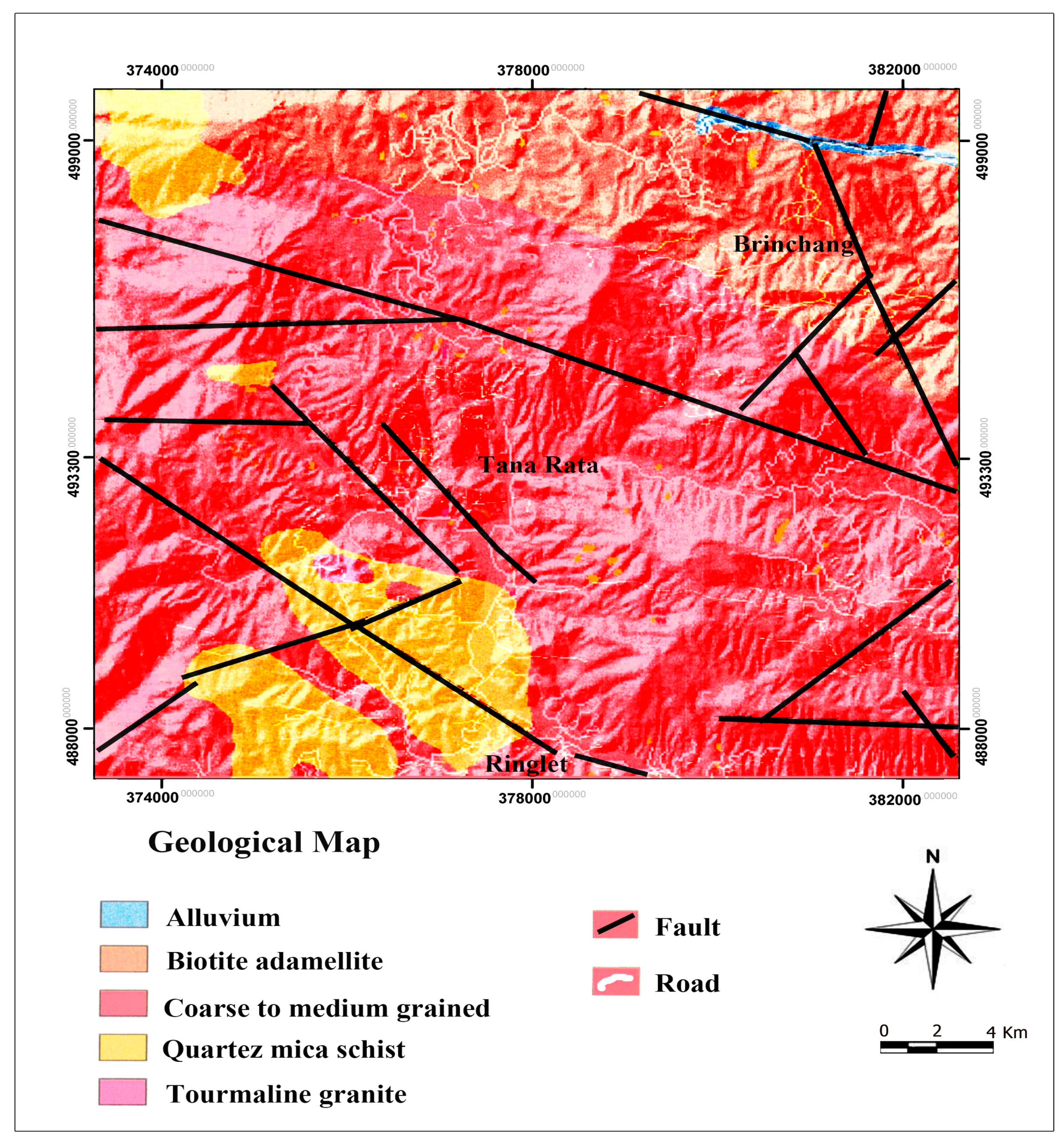
| Geology map | Lithology | Geological map obtained from the Mineral and Geosciences Department of Malaysia | ARC/INFO coverage | Lithology | 1:63,300 |
| Fault | Geological map obtained from the Mineral and Geosciences Department of Malaysia | Line | Distance to fault | 1:63,300 | |
| Road | Road | Topography map | Line | Distance to road | 1:25,000 |
| Land use type | Land use | SPOT 5 satellite image | ARC/INFO GRID | Land use | 15 m |
| Normalized difference Vegetation index (NDVI) | NDVI | SPOT 5 satellite image | ARC/INFO GRID | NDVI | 15 m |
| Rainfall | Rainfall | 30 years of historical rainfall data | GRID | Rainfall map (mm) | 1:25,000 |
| River | Rivers | AIRSAR DEM | ARC/INFO line coverage | Distance to river | 10-m pixel size |
| No. | Landslide Causal Factors | Classes | |
|---|---|---|---|
| Topographic factors | 1 | Slope (o) | (1) 0–10; (2) 10–20; (3) 20–30; (4) 30–40; (5) >40 |
| 2 | Aspect | (1) Flat; (2) north; (3) northeast; (4) east; (5) southeast; (6) south; (7) southwest; (8) west; (9) northwest | |
| Hydrological factors | 3 | Rainfall (mm) | (1) 2612–2661; (2) 2662–2678; (3) 2679–2694; (4) 2695–2708; (5) 2709–2719; (6) 2720–2731; (7) 2732–2743; (8) 2744–2754; (9) 2755–2764; (10) 2765–2781 |
| 4 | Distance to rivers (m) | (1) 0–50; (2) 50–100; (3) 100–150; (4) 150–200; (5) 200–300; (6) 300–500; (7) >500 | |
| Lithological factors | 5 | Lithology | (1) Metamorphic rock; (2) igneous rock |
| 6 | Distance to faults (m) | (1) 0–50; (2) 50–100; (3) 100–150; (4) 150–200; (5) 200–500; (6) >500 | |
| 7 | Soil | (1) Serong series; (2) alluvium-colluvium | |
| Land cover factors | 8 | Land use | (1) Grass; (2) primary forest; (3) rubber; (4) cutting; (5) secondary forest; (6) settlements; (7) agriculture area; (8) water body |
| 9 | NDVI | (1) [(−0.774)–(−0.613)]; (2) [(−0.618)–(−459)]; (3) [(−0.457)–(0.303)]; (4) [(−0.309)–(−0.139)]; (5) [(−0.144)–(0.012)]; (6) [0.015–0.174]; (7) [0.172–0.328]; (8) [0.322–0.491]; (9) [0.491–0.648]; (10) [0.641–0.809] | |
| Man-made factors | 10 | Distance to roads (m) | (1) 0–50; (2) 50–100; (3) 100–200; (4) 200–500; (5) >500 |
| Training | Validation | |||
|---|---|---|---|---|
| Train | SVM | IOE | SVM | IOE |
| True positive (TP) | 70 | 65 | 16 | 14 |
| True negative (TN) | 65 | 61 | 14 | 13 |
| False positive (FP) | 9 | 16 | 4 | 5 |
| False negative (FN) | 4 | 9 | 2 | 4 |
| Sensitivity (%) | 94.6 | 87.8 | 88.9 | 77.8 |
| Specificity (%) | 87.8 | 79.2 | 77.8 | 72.2 |
| Accuracy (%) | 91.2 | 83.4 | 83.3 | 75.0 |
| Kappa | 0.883 | 0.813 | 0.663 | 0.613 |
| AUROC | 0.896 | 0.826 | 0.845 | 0.826 |
| Factor | Class | Percentage of Domain | Percentage of Landslide | Pij | (Pij) | Hj | Hjmax | Ij | Wj |
|---|---|---|---|---|---|---|---|---|---|
| Slope (°) | 0–10 | 17.63 | 9.07 | 0.51 | 0.107 | 1.085 | 1.629 | 0.962 | 0.910 |
| 10–20 | 19.45 | 14.51 | 0.75 | 0.158 | |||||
| 20–30 | 21.71 | 26.12 | 1.20 | 0.253 | |||||
| 30–40 | 25.31 | 37.84 | 1.49 | 0.315 | |||||
| >40 | 15.90 | 12.46 | 0.78 | 0.164 | |||||
| Aspect | Flat | 0.00 | 0.00 | 0.00 | 0.00 | 1.726 | 1.871 | 0.948 | 0.840 |
| North | 6.09 | 8.14 | 1.34 | 0.167 | |||||
| Northeast | 16.41 | 14.39 | 0.88 | 0.110 | |||||
| East | 19.01 | 21.54 | 1.13 | 0.141 | |||||
| Southeast | 18.93 | 17.28 | 0.91 | 0.114 | |||||
| South | 10.21 | 9.46 | 0.93 | 0.116 | |||||
| Southwest | 7.58 | 3.52 | 0.46 | 0.057 | |||||
| West | 10.15 | 9.31 | 0.92 | 0.115 | |||||
| Northwest | 11.62 | 16.36 | 1.41 | 0.176 | |||||
| Soil | Serong series | 38.87 | 38.05 | 0.98 | 0.492 | 1.471 | 1.938 | 1.178 | 1.172 |
| Alluvium-colluvium | 61.13. | 61.95 | 1.02 | 0.507 | |||||
| Lithology | Metamorphic rock | 58.63 | 59.72 | 1.11 | 0.512 | 1.718 | 1.995 | 1.133 | 1.127 |
| Igneous rock | 41.37 | 40.28 | 0.97 | 0.487 | |||||
| NDVI | −0.774–−0.613 | 0.00 | 0.00 | 0.00 | 0.000 | 0.701 | 0.955 | 0.220 | 0.184 |
| −0.618–−0.459 | 6.41 | 5.23 | 0.81 | 0.096 | |||||
| −0.457–−0.303 | 8.72 | 7.93 | 0.91 | 0.108 | |||||
| −0.309–−0.139 | 12.16 | 10.33 | 0.85 | 0.101 | |||||
| −0.144–0.012 | 26.28 | 29.95 | 1.14 | 0.136 | |||||
| 0.015–0.174 | 3.04 | 2.01 | 0.66 | 0.078 | |||||
| 0.172–0.328 | 4.96 | 5.11 | 1.03 | 0.123 | |||||
| 0.332–0.491 | 7.21 | 6.76 | 0.94 | 0.112 | |||||
| 0.491–0.648 | 11.70 | 10.55 | 0.90 | 0.107 | |||||
| 0.641–0.809 | 19.52 | 22.13 | 1.13 | 0.135 | |||||
| Land use | Grass | 3.62 | 2.73 | 0.75 | 0.099 | 1.735 | 1.899 | 0.985 | 0.932 |
| Primary forest | 8.71 | 12.44 | 0.74 | 0.097 | |||||
| Rubber | 8.11 | 7.45 | 0.92 | 0.121 | |||||
| Cutting | 21.79 | 20.47 | 0.94 | 0.125 | |||||
| Secondary forest | 19.62 | 18.43 | 0.93 | 0.122 | |||||
| Settlements | 18.14 | 17.76 | 0.98 | 0.129 | |||||
| Agriculture area | 4.46 | 6.10 | 1.37 | 0.180 | |||||
| Water body | 15.55 | 14.62 | 0.94 | 0.124 | |||||
| Rainfall (mm/year) | 2612–2661 | 16.57 | 15.87 | 0.96 | 0.079 | 1.766 | 2.239 | 1.450 | 1.753 |
| 2662–1681 | 6.20 | 6.18 | 0.99 | 0.081 | |||||
| 2679–2694 | 6.77 | 6.98 | 1.03 | 0.085 | |||||
| 2695–2708 | 18.12 | 19.63 | 1.09 | 0.090 | |||||
| 2709–2719 | 8.66 | 7.17 | 0.83 | 0.068 | |||||
| 2720–2731 | 10.07 | 8.23 | 0.82 | 0.067 | |||||
| 2732–2743 | 11.11 | 9.55 | 0.86 | 0.071 | |||||
| 2744–2754 | 13.95 | 12.41 | 0.89 | 0.073 | |||||
| 2755–2764 | 7.09 | 9.10 | 1.28 | 0.105 | |||||
| 2765–2781 | 2.46 | 4.88 | 3.34 | 0.276 | |||||
| Distance to faults (m) | 0–50 | 11.75 | 19.23 | 1.07 | 0.257 | 1.378 | 1.548 | 0.657 | 0.692 |
| 50–100 | 21.19 | 22.64 | 1.05 | 0.169 | |||||
| 100–150 | 9.04 | 9.41 | 1.04 | 0.164 | |||||
| 150–200 | 10.98 | 11.79 | 1.07 | 0.163 | |||||
| 200–500 | 29.71 | 25.81 | 0.87 | 0.137 | |||||
| >500 | 17.33 | 11.12 | 0.64 | 0.101 | |||||
| Distance to rivers (m) | 0–50 | 11.40 | 12.91 | 1.23 | 0.160 | 2.558 | 2.633 | 1.661 | 1.670 |
| 50–100 | 19.41 | 21.01 | 1.08 | 0.153 | |||||
| 100–150 | 17.99 | 18.65 | 1.03 | 0.146 | |||||
| 150–200 | 3.61 | 3.72 | 1.03 | 0.145 | |||||
| 200–300 | 9.33 | 8.97 | 0.96 | 0.136 | |||||
| 300–500 | 29.77 | 27.09 | 0.91 | 0.129 | |||||
| >500 | 8.49 | 7.65 | 0.90 | 0.127 | |||||
| Distance to roads (m) | 0–50 | 22.01 | 37.64 | 1.17 | 0.302 | 1.611 | 1.759 | 0.843 | 0.793 |
| 50–100 | 19.26 | 18.82 | 0.98 | 0.173 | |||||
| 100–150 | 15.52 | 11.76 | 0.76 | 0.135 | |||||
| 150–200 | 13.84 | 10.61 | 0.76 | 0.134 | |||||
| 200–500 | 17.98 | 12.94 | 0.72 | 0.127 | |||||
| >500 | 11.39 | 8.23 | 0.72 | 0.123 |
| Landslide Models | Mean Ranks | χ2 | Significance |
|---|---|---|---|
| SVM | 2.01 | 35.286 | 0.000 |
| IOE | 1.65 |
| Pairwise Comparison | Positive | Negative | Z (Value) | p (Value) | Significance |
|---|---|---|---|---|---|
| SVM vs. IOE | 45 | 12 | −10.235 | 0.000 | Yes |
© 2018 by the authors. Licensee MDPI, Basel, Switzerland. This article is an open access article distributed under the terms and conditions of the Creative Commons Attribution (CC BY) license (http://creativecommons.org/licenses/by/4.0/).
Share and Cite
Tien Bui, D.; Shahabi, H.; Shirzadi, A.; Chapi, K.; Alizadeh, M.; Chen, W.; Mohammadi, A.; Ahmad, B.B.; Panahi, M.; Hong, H.; et al. Landslide Detection and Susceptibility Mapping by AIRSAR Data Using Support Vector Machine and Index of Entropy Models in Cameron Highlands, Malaysia. Remote Sens. 2018, 10, 1527. https://doi.org/10.3390/rs10101527
Tien Bui D, Shahabi H, Shirzadi A, Chapi K, Alizadeh M, Chen W, Mohammadi A, Ahmad BB, Panahi M, Hong H, et al. Landslide Detection and Susceptibility Mapping by AIRSAR Data Using Support Vector Machine and Index of Entropy Models in Cameron Highlands, Malaysia. Remote Sensing. 2018; 10(10):1527. https://doi.org/10.3390/rs10101527
Chicago/Turabian StyleTien Bui, Dieu, Himan Shahabi, Ataollah Shirzadi, Kamran Chapi, Mohsen Alizadeh, Wei Chen, Ayub Mohammadi, Baharin Bin Ahmad, Mahdi Panahi, Haoyuan Hong, and et al. 2018. "Landslide Detection and Susceptibility Mapping by AIRSAR Data Using Support Vector Machine and Index of Entropy Models in Cameron Highlands, Malaysia" Remote Sensing 10, no. 10: 1527. https://doi.org/10.3390/rs10101527
APA StyleTien Bui, D., Shahabi, H., Shirzadi, A., Chapi, K., Alizadeh, M., Chen, W., Mohammadi, A., Ahmad, B. B., Panahi, M., Hong, H., & Tian, Y. (2018). Landslide Detection and Susceptibility Mapping by AIRSAR Data Using Support Vector Machine and Index of Entropy Models in Cameron Highlands, Malaysia. Remote Sensing, 10(10), 1527. https://doi.org/10.3390/rs10101527