
Decision Support Tools and Strategies to Simulate Forest Landscape Evolutions Integrating Forest Owner Behaviour: A Review from the Case Studies of the European Project, INTEGRAL

 ,
, 
 ,
, 
 ,
,  , , ,
, , ,  ,
,  , ,
, ,  and
and
Abstract
:1. Introduction
2. Descriptions of the Decision Support System (DSS) Used for Landscape Simulation within INTEGRAL Case Studies
2.1. The Simulated Forest Management Programmes
2.2. The Evolution Engines and Landscape Simulation Tools
2.3. Forests Growth Models: The Key Evolution Engines
- The yield tables (included in REMSOFT, PINEA and CASTANEA models) are derived from equations, from data collection in the field or from stem analysis. These tables provide year-by-year growing stock value and harvested volumes for a given thinning regime. The number of yield tables needed depends on a combination of site index and thinning regime in a given area. This tool is robust and appropriate for a very standard management scheme and for homogenous sites with low fertility variation.
- The stand empirical growth models (Fagacées, Lemoine, EFISCEN, Kupolis) and matrix models (EFISCEN) comprise equations providing evolution of height and basal area (or biomass) over time for a forest stand. They can be used to compare the impact of various thinning regimes.
- The individual tree growth models can cope with a large diversity of thinning regimes providing outputs related to growth and tree shape. These models are either tree distance independent (Heureka, Pinaster, PBIRROL, SUBER and MNL) or tree distance dependent (SIBYLA, SILVA). Therefore, in the former case, the models will provide the same result whatever the shape of the parcel or the tree distribution within the stand; whereas in the latter uneven aged stands and differences based on initial stand structure or parcel shapes can be simulated.
- The latest developments in modelling allow a combination of growth models and process based (LandClim) models to be used. These can theoretically simulate the evolution of a stand whatever thinning regime is applied, based on the competition between trees, climate and site characteristics. Recent empirical growth models, such as SIBYLA, can also take climate change into account by adjusting the site index according to climatic variables, rather than describing the light and water processes.
2.4. Specific Growth Model Characteristics Required for Certain Scenarios
2.4.1. Mortality
2.4.2. Hazards
2.4.3. Global Change in Models
2.5. The DSS: The Integrative Tools to Run Simulation at Landscape Level
2.5.1. The Need for an Integrative Tool
2.5.2. Constraints Rules at the Landscape Level
3. The Strategies to Cope with the Tree Species Issue
4. The Stand Structure and Alternative Management Option Issues
5. The Input and Output Data Sets Required to Run Landscape Simulations or Expected from the DSS
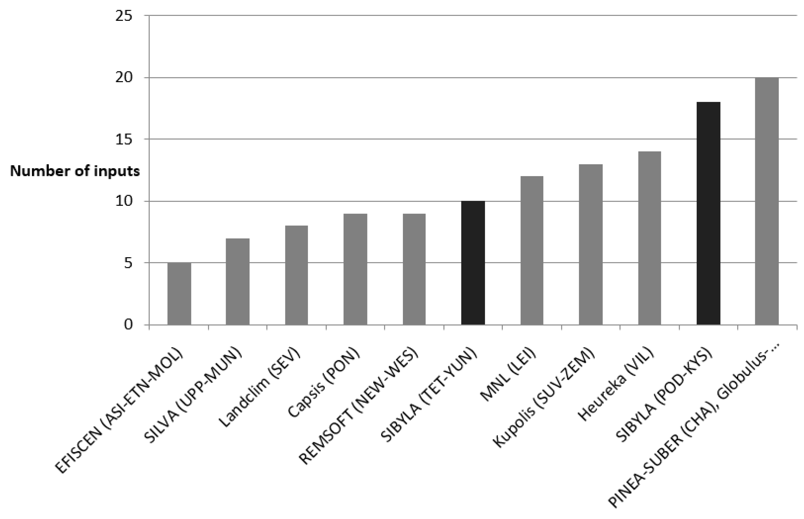
5.1. Input Data Required by the DSS
- The more classical definition of the thinning regime is a calendar listing operations at a given age or the periodicity of operations. This leads to a very low flexibility depending on the heterogeneity of the environment,
- Other thinning regimes are driven by dendrometric thresholds that trigger certain actions: with SIMMEM, relative density triggers thinning and max diameter clear-cut, with ForClim, total biomass or diameter trigger thinning,
- Some of the models were also able to carry out specific optimisation by adjusting the thinning regime stand by stand to optimise a species composition or a net value depending on the site.
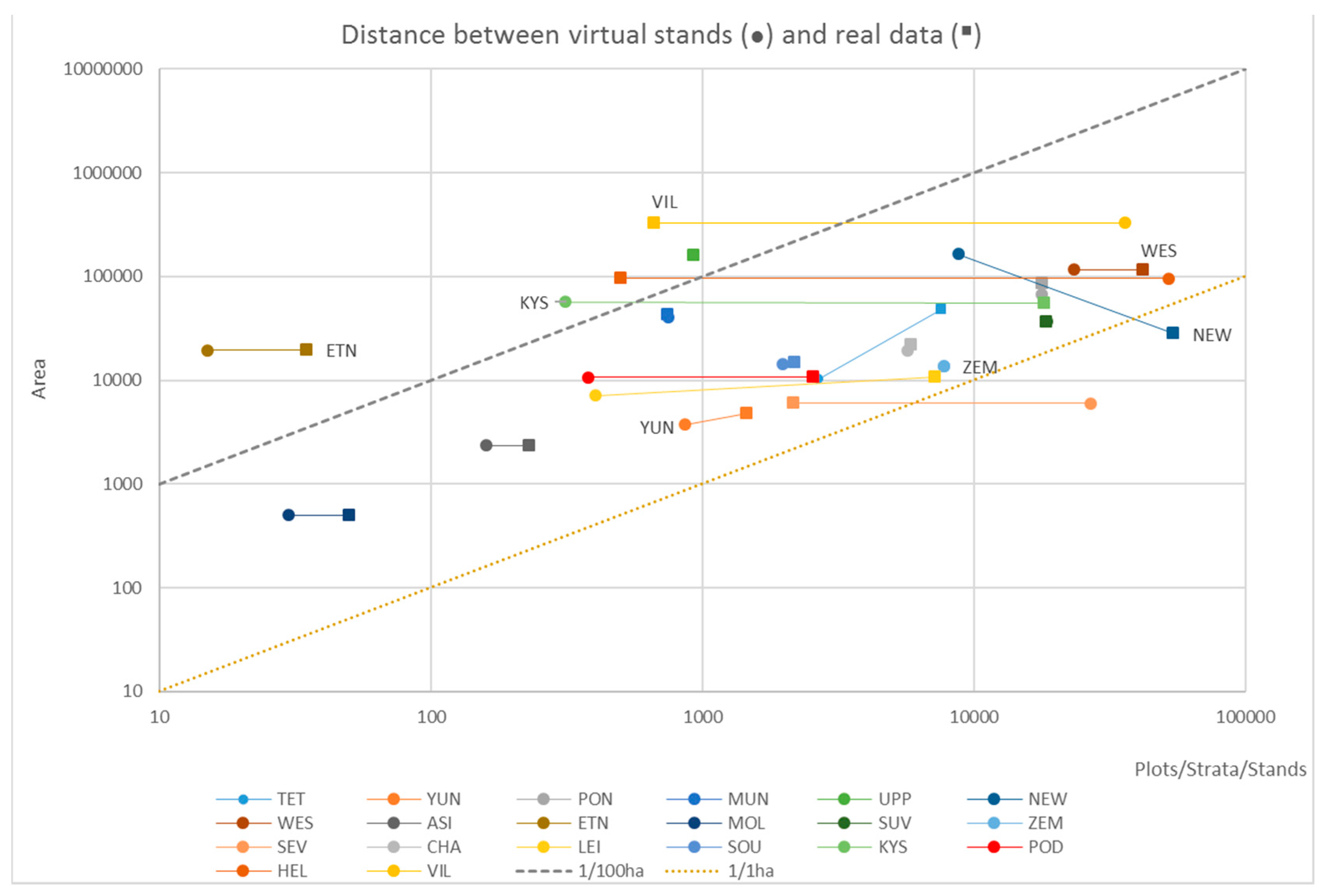
5.2. Sources of Input Data
5.3. Outputs Provided by the DSS for the Case Studies
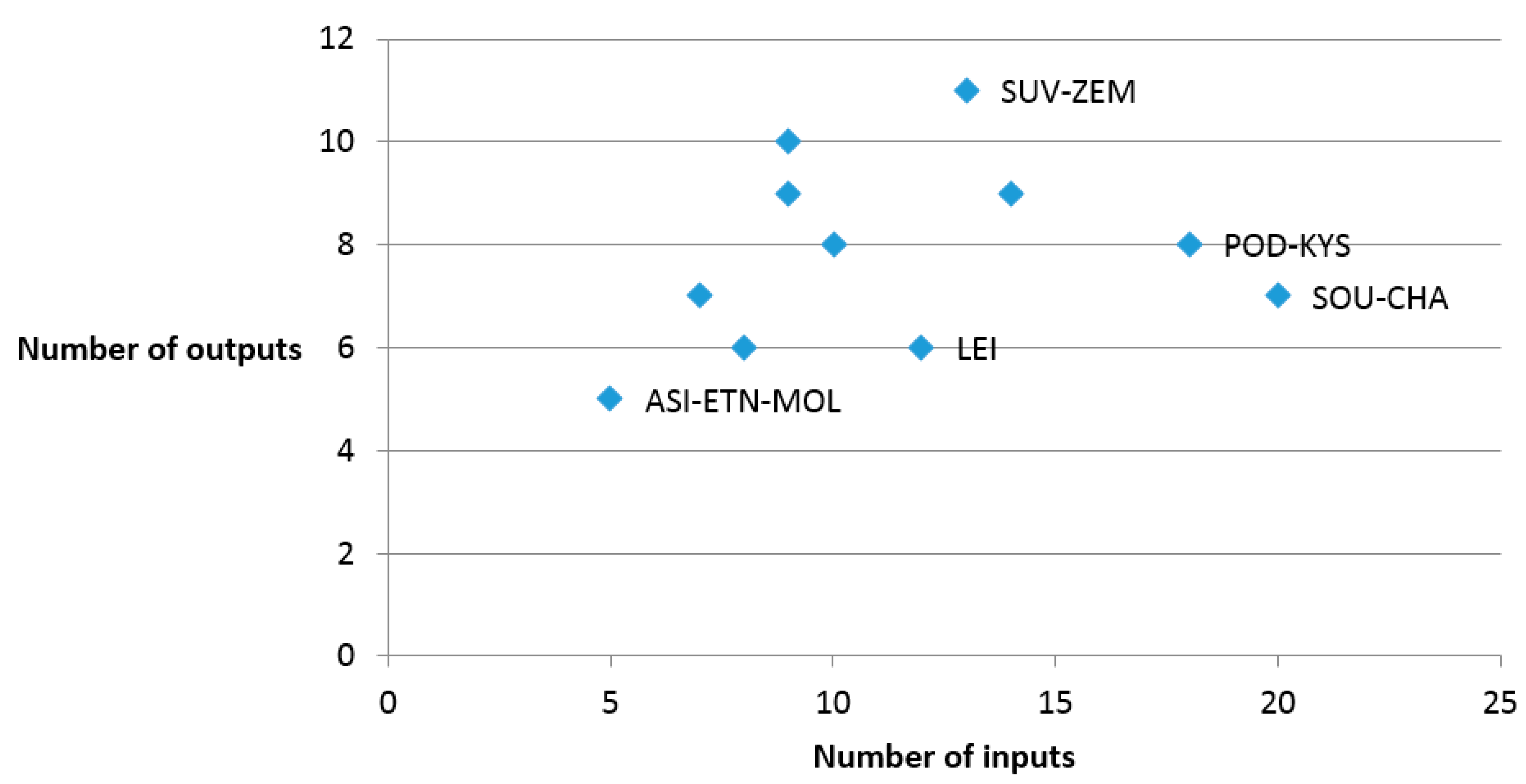
5.4. Relationship between Inputs and Outputs
6. Discussion
6.1. Strengths and Weaknesses of the Listed Tools
6.2. How Can the Appropriate Tool Be Selected to Run a Landscape Simulation in a Given Region?
7. Conclusions
Acknowledgments
Author Contributions
Conflicts of Interest
Abbreviations
| CC | Climate Change |
| CO2 | Carbon dioxide |
| DEM | Digital Elevation Model |
| FMA | Forest Management Action |
| FMP | Forest Management Plan |
| FO | Forest Owner |
| FS | Forest Service |
| IGN | Institut national de l’information géographique et forestière |
| IPCC | The Intergovernmental Panel on Climate Change |
| KNMI | The Royal Netherlands Meteorological Institute |
| MAI | Mean Annual Increment |
| NFC | National Forest Centre |
| NFI | National Forest Inventory |
| NFIS | National Forest Information System |
| NOx | Nitrogen oxide |
| ONF | Office National des Forêts |
| RSD | Remote Sensing Data |
| SRTM | Shuttle Radar Topographic Mission |
References
- Gardner, T.A.; Barlow, J.; Chazdon, R.; Ewers, R.M.; Harvey, C.A.; Peres, C.A.; Sodhi, N.S. Prospects for tropical forest biodiversity in a human-modified world. Ecol. Lett. 2009, 12, 561–582. [Google Scholar] [CrossRef] [PubMed]
- Thompson, I.D.; Okabe, K.; Parrotta, J.A.; Brockerhoff, E.; Jactel, H.; Forrester, D.I.; Taki, H. Biodiversity and ecosystem services: Lessons from nature to improve management of planted forests for REDD-plus. Biodivers. Conserv. 2014, 23, 2613–2635. [Google Scholar] [CrossRef]
- Živojinović, I.; Weiss, G.; Lidestav, G.; Feliciano, D.; Hujala, T.; Dobšinská, Z.; Lawrence, A.; Nybakk, E.; Quiroga, S.; Schraml, U. Forest Land Ownership Change in Europe. Cost Action FP120 FACEMAP Country Reports; University of Natural Resources and Life Sciencesn (BOKU): Vienna, Austria, 2015. [Google Scholar]
- FOREST EUROPE. State of Europe’s Forests. 2015. Available online: http://www.foresteurope.org/docs/fullsoef2015.pdf (accessed on 12 April 2017).
- Duelli, P.; Obrist, M.K. Biodiversity indicators: The choice of values and measures. Agric. Ecosyst. Environ. 2003, 98, 87–98. [Google Scholar] [CrossRef]
- Pukkala, T.; Nuutinen, T.; Kangas, J. Integrating scenic and recreational amenities into numerical forest planning. Landsc. Urban Plan. 1995, 32, 185–195. [Google Scholar] [CrossRef]
- Orazio, C.; Tomé, M.; Colin, A.; Diez Casero, J.; Jactel, H.; Mendes, A.; Martinez, I. FORSEE PROJECT: A Network of 10 Pilot Zones to Test and Improve Criteria and Indicators for Sustainable Forest Management at Regional Level in Atlantic European Countries; Rationale and Workplan Interim report; IEFC: Cestas, France, 2006. [Google Scholar]
- INTEGRAL Project Consortium. Future-Oriented Integrated Management of European Forest Landscapes. Available online: http://www.integral-project.eu/ (accessed on 13 December 2016).
- Biber, P.; Borges, J.; Moshammer, R.; Barreiro, S.; Botequim, B.; Brodrechtová, Y.; Brukas, V.; Chirici, G.; Cordero-Debets, R.; Corrigan, E.; et al. How Sensitive Are Ecosystem Services in European Forest Landscapes to Silvicultural Treatment? Forests 2015, 6, 1666–1695. [Google Scholar] [CrossRef]
- Sallustio, L.; Quatrini, V.; Geneletti, D.; Corona, P.; Marchetti, M. Assessing land take by urban development and its impact on carbon storage: Findings from two case studies in Italy. Environ. Impact Assess. Rev. 2015, 54, 80–90. [Google Scholar] [CrossRef]
- Carlsson, J.; Eriksson, L.O.; Öhman, K.; Nordström, E.-M. Combining scientific and stakeholder knowledge in future scenario development—A forest landscape case study in northern Sweden. For. Policy Econ. 2015, 61, 122–134. [Google Scholar] [CrossRef]
- Ferreira, L.; Constantino, M.F.; Borges, J.G.; Garcia-Gonzalo, J. Addressing Wildfire Risk in a Landscape-Level Scheduling Model: An Application in Portugal. For. Sci. 2015, 61, 266–277. [Google Scholar] [CrossRef]
- Orazio, C.; Cordero, R.; Hautdidier, B.; Meredieu, C.; Vallet, P. Simulation de l’évolution de la dynamique forestière dans les Landes de Gascogne sous différents scénarios socioéconomiques. Rev. For. Fr. 2015, 493–514. (In French) [Google Scholar] [CrossRef]
- Sergent, A.; Hautdidier, B.; Deuffic, P.; Banos, V. WP 3.2 INTEGRAL National Case Study Reports, France. Case Study Area, Pontenx Description. Available online: https://forestwiki.jrc.ec.europa.eu/integral/index.php/Pontenx (accessed on 22 August 2016).
- Orazio, C.; Tomé, M.; Meredieu, C. FORMODELS, Register of Models for Forest. Available online: http://www.efiatlantic.efi.int/portal/databases/formodels/ (accessed on 9 December 2016).
- Fabrika, M.; Ďurský, J. Algorithms and software solution of thinning models for SIBYLA growth simulator. J. For. Sci. 2005, 51, 431–445. [Google Scholar]
- Lemoine, B. Growth and yield of maritime pine (Pinus pinaster Ait): The average dominant tree of the stand. Ann. Sci. For. 1991, 48, 593–611. [Google Scholar] [CrossRef]
- Le Moguédec, G.; Dhôte, J.-F. Fagacées: A tree-centered growth and yield model for sessile oak (Quercus petraea L.) and common beech (Fagus sylvatica L.). Ann. For. Sci. 2012, 69, 257–269. [Google Scholar] [CrossRef]
- Dufour-Kowalski, S.; Courbaud, B.; Dreyfus, P.; Meredieu, C.; de Coligny, F. Capsis: An open software framework and community for forest growth modelling. Ann. For. Sci. 2012, 69, 221–233. [Google Scholar] [CrossRef]
- Cucchi, V.; de Coligny, F.; Cordonnier, T.; Vallet, P. SIMMEM Simulateur Multi-Modules Pour L’échelle Massif. Available online: http://capsis.cirad.fr/capsis/help/simmem (accessed on 22 August 2016).
- Pretzsch, H.; Biber, P.; Ďurský, J. The single tree-based stand simulator SILVA: Construction, application and evaluation. For. Ecol. Manag. 2002, 162, 3–21. [Google Scholar] [CrossRef]
- Remsoft Forestry. Available online: http://www.remsoft.com/forestry.php (accessed on 12 July 2016).
- Sallnäs, O. A Matrix Growth Model of the Swedish Forest; Studia forestalia suecica; Swedish University of Agricultural Sciences: Uppsala, Sweden, 1990. [Google Scholar]
- Schelhaas, M.-J.; Eggers, J.; Lindner, M.; Nabuurs, G.-J.; Pussinen, A.; Päivinen, R.; Schuck, A.; Verkerk, P.J.; van der Werf, D.C.; Zudin, S. Model Documentation for the European Forest Information Scenario Model (EFISCEN 3.1.3); EFI Technical Report 26; Alterra: Wageningen, The Netherlands, 2007. [Google Scholar]
- Petrauskas, E.; Kuliešis, A. Scenario-Based Analysis of Possible Management Alternatives for Lithuanian Forests in the 21 st Century. Balt. For. 2004, 10, 72–82. [Google Scholar]
- Schumacher, S.; Bugmann, H.; Mladenoff, D.J. Improving the formulation of tree growth and succession in a spatially explicit landscape model. Ecol. Model. 2004, 180, 175–194. [Google Scholar] [CrossRef]
- Hengeveld, G.M.; Didion, M.; Clerkx, S.; Elkin, C.; Nabuurs, G.-J.; Schelhaas, M.-J. The landscape-level effect of individual-owner adaptation to climate change in Dutch forests. Reg. Environ. Chang. 2015, 15, 1515–1529. [Google Scholar] [CrossRef]
- Barreiro, S.; Garcia-Gonzalo, J.; Borges, J.; Tomé, M.; Marques, S. SADfLOR Tutorial. A Web-Based Forest and Natural Resources Decision Support System (Work in Progress); FORCHANGE, ISA: Lisboa, Portugal, 2013; p. 39. [Google Scholar]
- Garcia-Gonzalo, J.; Borges, J.G.; Palma, J.H.N.; Zubizarreta-Gerendiain, A. A decision support system for management planning of Eucalyptus plantations facing climate change. Ann. For. Sci. 2014, 71, 187–199. [Google Scholar] [CrossRef]
- Barreiro, S.; Rua, J.; Tomé, M. StandsSIM-MD: A Management Driven forest SIMulator. For. Syst. 2016, 25, eRC07. [Google Scholar] [CrossRef]
- Wikström, P.; Edenius, L.; Elfving, B.; Eriksson, L.O.; Lämås, T.; Sonesson, J.; Öhman, K.; Wallerman, J.; Waller, C.; Klintebäck, F. The Heureka forestry decision support system: An overview. Int. J. Math. Comput. For. Nat. Resour. Sci. 2011, 3, 87–95. [Google Scholar]
- Salas, C.; Gregoire, T.G.; Craven, D.J.; Gilabert, H. Modelación del crecimiento de bosques: Estado del arte. Bosque Valdivia 2016, 37, 3–12. [Google Scholar] [CrossRef]
- Pretzsch, H.; Forrester, D.I.; Rötzer, T. Representation of species mixing in forest growth models. A review and perspective. Ecol. Model. 2015, 313, 276–292. [Google Scholar] [CrossRef]
- Charru, M.; Seynave, I.; Morneau, F.; Rivoire, M.; Bontemps, J.-D. Significant differences and curvilinearity in the self-thinning relationships of 11 temperate tree species assessed from forest inventory data. Ann. For. Sci. 2012, 69, 195–205. [Google Scholar] [CrossRef]
- Sales Luis, J.F.; Fonseca, T.F. The allometric model in the stand density management of Pinus pinaster Ait. in Portugal. Ann. For. Sci. 2004, 61, 807–814. [Google Scholar] [CrossRef]
- Hanewinkel, M.; Hummel, S.; Albrecht, A. Assessing natural hazards in forestry for risk management: A review. Eur. J. For. Res. 2011, 130, 329–351. [Google Scholar] [CrossRef]
- Carvalho, M.J.; Melo-Gonçalves, P.; Teixeira, J.C.; Rocha, A. Regionalization of Europe based on a K-Means Cluster Analysis of the climate change of temperatures and precipitation. Phys. Chem. Earth Parts ABC 2016, 94, 22–28. [Google Scholar] [CrossRef]
- Fontes, L.; Bontemps, J.-D.; Bugmann, H.; Van Oijen, M.; Gracia, C.; Kramer, K.; Lindner, M.; Rötzer, T.; Skovsgaard, J.P. Models for supporting forest management in a changing environment. For. Syst. 2011, 3, 8. [Google Scholar] [CrossRef]
- GIS-National Forest Centre. Available online: http://gis.nlcsk.org/lgis/ (accessed on 15 December 2016).
- Pachauri, R.K.; Mayer, L. Climate Change 2014: Synthesis Report; Intergovernmental Panel on Climate Change, Ed.; Intergovernmental Panel on Climate Change: Geneva, Switzerland, 2015. [Google Scholar]
- Fabrika, M. Simulátor Biodynamiky Lesa SIBYLA, Koncepcia, Konštrukcia a Programové Riešenie (Simulator of Forest Biodynamics SIBYLA, Framework, Construction and Software Solution). Habilitation Thesis, Technical University in Zvolen, Zvolen, Slovakia, 2005. [Google Scholar]
- ForestPortal Informačné Listy LTIS. Available online: http://www.forestportal.sk/lesne-hospodarstvo/informacie-o-lesoch/trhove-spravodajstvo/Pages/informacne-listy-ltis.aspx (accessed on 15 December 2016).
- Pauliukevičius, G.; Kenstavičius, J. Ekologiniai Miškų Teritorinio Išdėstymo Pagrindai [Ecologic Fundamentals of Spatial Forest Distribution]. Vilnius 1995, 1, 194. (In Lithuanian) [Google Scholar]
- Edwards, D.M.; Jay, M.; Jensen, F.S.; Lucas, B.; Marzano, M.; Montagné, C.; Peace, A.; Weiss, G. Public Preferences Across Europe for Different Forest Stand Types as Sites for Recreation. Ecol. Soc. 2012, 17. [Google Scholar] [CrossRef]
- D1-819/3D-790 Harmonized Methodology for Collecting Data and Calculating the Amounts of Absorbed and Emitted Green-House Gases in the Sectors of Land-Use Changes and Forestry. Available online: https://www.e-tar.lt/portal/en/legalAct/TAR.0ACB228423D2 (accessed on 15 December 2016).
- Patrício, M.S. Análise da Potencialidade Produtiva do Castanheiro em Portugal; Tese de Doutoramento em Engenharia Florestal, Universidade Técnica de Lisboa, Instituto Superior de Agronomia: Lisboa, Portugal, 2006. (In Portuguese) [Google Scholar]
- Garcia-Gonzalo, J.; Palma, J.; Freire, J.; Tomé, M.; Mateus, R.; Rodriguez, L.C.E.; Bushenkov, V.; Borges, J.G. A decision support system for a multi stakeholder’s decision process in a Portuguese National Forest. For. Syst. 2013, 22, 359. [Google Scholar] [CrossRef]
- Belouard, T.; Py, N.; Maillet, G.; Guyon, D.; Meredieu, C.; Pausader, M.; Champion, N. Pinastéréo—Estimation de la hauteur dominante et de la biomasse forestière dans le massif des Landes de Gascogne à partir d’images stéréoscopiques Pléiades. Rev. Fr. Photogramm. Télédétec. 2015, 209, 133–139. (In French) [Google Scholar]
- Vega, C.; Stonge, B. Height growth reconstruction of a boreal forest canopy over a period of 58 years using a combination of photogrammetric and lidar models. Remote Sens. Environ. 2008, 112, 1784–1794. [Google Scholar] [CrossRef]
- Muys, B.; Hynynen, J.; Palahi, M.; Lexer, M.J.; Fabrika, M.; Pretzsch, H.; Gillet, F.; Briceño, E.; Nabuurs, G.J.; Kint, V. Simulation tools for decision support to adaptive forest management in Europe. For. Syst. 2011, 3, 86. [Google Scholar] [CrossRef]
- Pastorella, F.; Borges, J.; De Meo, I. Usefulness and perceived usefulness of Decision Support Systems (DSSs) in participatory forest planning: The final users’ point of view. iForest 2016, 9, 422–429. [Google Scholar] [CrossRef]
- Packalen, T.; Marques, A.; Rasinmäki, J.; Rosset, C.; Mounir, F.; Rodriguez, L.C.E.; Nobre, S.R. Review. A brief overview of forest management decision support systems (FMDSS) listed in the FORSYS wiki. For. Syst. 2013, 22, 263. [Google Scholar] [CrossRef]
- Pezdevšek Malovrh, Š.; Kurttila, M.; Hujala, T.; Kärkkäinen, L.; Leban, V.; Lindstad, B.H.; Peters, D.M.; Rhodius, R.; Solberg, B.; Wirth, K.; et al. Decision support framework for evaluating the operational environment of forest bioenergy production and use: Case of four European countries. J. Environ. Manag. 2016, 180, 68–81. [Google Scholar] [CrossRef] [PubMed]
- ForestDSS.org, Community of Practice Forest Management Decision Support Systems. Available online: http://www.forestdss.org/CoP/ (accessed on 15 December 2016).
- Santopuoli, G.; Requardt, A.; Marchetti, M. Application of indicators network analysis to support local forest management plan development: A case study in Molise, Italy. iForest 2012, 5, 31–37. [Google Scholar] [CrossRef]
- Pereira, H.M.; Ferrier, S.; Walters, M.; Geller, G.N.; Jongman, R.H.G.; Scholes, R.J.; Bruford, M.W.; Brummitt, N.; Butchart, S.H.M.; Cardoso, A.C.; et al. Essential Biodiversity Variables. Science 2013, 339, 277–278. [Google Scholar] [CrossRef] [PubMed]
- Vacik, H.; Lexer, M.J. Past, current and future drivers for the development of decision support systems in forest management. Scand. J. For. Res. 2014, 29, 2–19. [Google Scholar] [CrossRef]


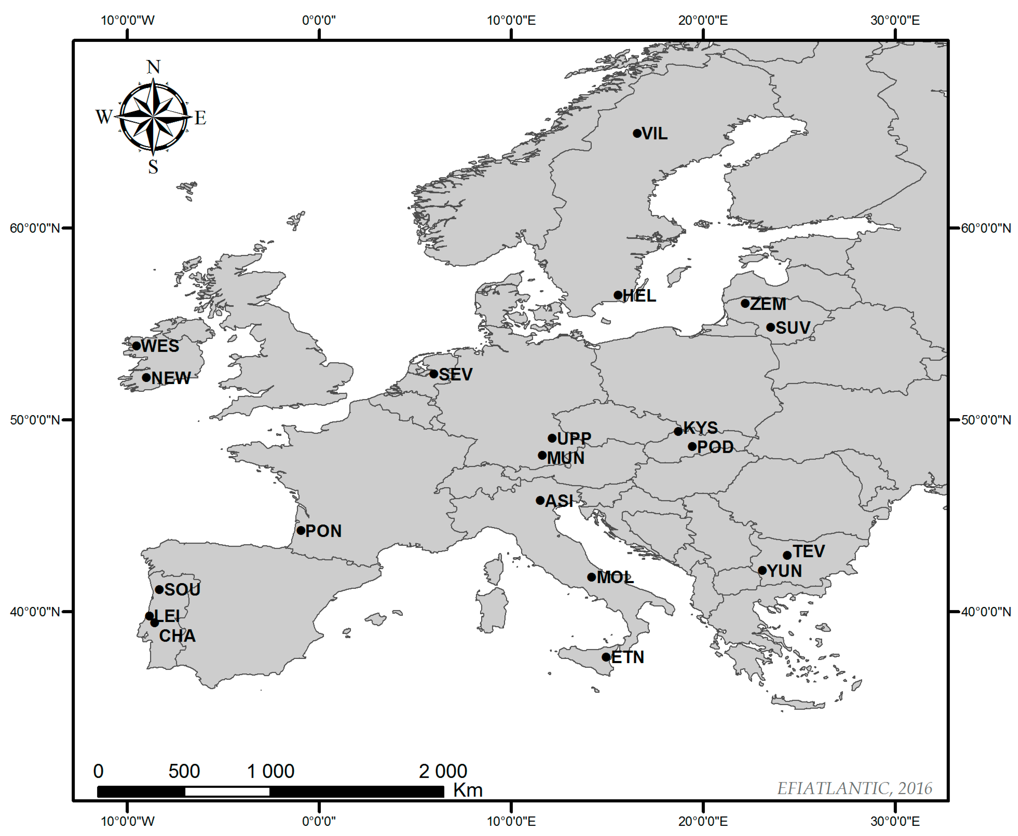
| Country | Case Study Area (CSA) | CSA Acronym | Forest Region in Europe | Latitude | Longitude | Total Area (ha) | Forest Area (ha) | Number of Trees Species in CSA | Main Tree Species (>10% of Volumes in the Area) |
|---|---|---|---|---|---|---|---|---|---|
| Bulgaria | Teteven | TET | E | 42°55′N | 24°25′E | 69,700 | 47,812 | 29 (NFI) | FASY, CAOR, QUCE, PISY |
| Bulgaria | Yundola | YUN | E | 42°01′N | 23°06′E | 5211 | 4750 | 13 (NFI) | ABAL, FASY |
| France | Pontenx | PON | CW | 44°12′N | 00°55′W | 101,000 | 86,000 | 8 | PIPI, QUPY, QURO |
| Germany | Munich South | MUN | CW | 48°08′N | 11°34′E | 60,000 | 43,200 | 38 (NFI) | PIAB, PISY, FASY |
| Germany | Upper Palatinate | UPP | CW | 49°01′N | 12°05′E | 300,000 | 159,000 | 36 (NFI) | PIAB, FASY |
| Ireland | Newmarket | NEW | NW | 52°12′N | 09°00′W | 187,820 | 28,000 | 15 | PISI, PIAB, PICO, PISY, LADE, LAKA, PSME, QUPE, FASY |
| Ireland | Western Peatlands | WES | NW | 53°48′N | 09°31′W | 1,060,000 | 116,000 | 16 | PISI, PIAB, PICO, PISY, LADE, LAKA, PSME, QUPE, FASY |
| Italy | Asiago | ASI | S | 45°52′N | 11°31′E | 103,000 | 2350 | 3 | PIAB, ABAL, FASY |
| Italy | Etna | ETN | S | 37°45′N | 14°59′E | 25,300 | 19,500 | 3 | ABAL, QUCE, Fagus spp. |
| Italy | Molise | MOL | S | 41°40′N | 14°15′E | 600 | 501 | 3 | QUPU, QUIL, PINI plantations, ABAL native forests |
| Lithuania | Suvalkija | SUV | E | 54°45′N | 23°30′E | 66,000 | 36,785 | 15 | PISY, PIAB, BEPU, BEVE, ALGL |
| Lithuania | Zemaitija | ZEM | E | 55°59′N | 22°15′E | 37,900 | 13,674 | 16 | PISY, PIAB, BEPU, BEVE |
| The Netherlands | South East Veluwe | SEV | W | 52°13′N | 5°58′E | 8000 | 6000 | 23 | FASY, PISY, PSME, QURO |
| Portugal | Chamusca | CHA | S | 39°21′N | 8°29′W | 74,600 | 21,978 | 4 | EUGL, PIPI, PIPIN, QUSU |
| Portugal | Leiria | LEI | S | 39°45′N | 8°48′W | 75,200 | 10,768 | 1 | PIPI |
| Portugal | Sousa | SOU | S | 41°04′N | 8°15′W | 48,900 | 14,832 | 3 | EUGL, PIPI |
| Slovakia | Kysuce | KYS | E | 49°22′N | 18°44′E | 98,222 | 55,609 | 5 | PIAB, FASY, ABAL, Quercus spp., PISY |
| Slovakia | Podpol’anie | POD | E | 48°34′N | 19°30′E | 21,255 | 10,627 | 5 | PIAB, FASY, ABAL, Quercus spp., PISY |
| Sweden | Helgeå | HEL | N | 56°25′N | 15°42′E | 120,000 | 96,000 | 5 | PIAB, PISY |
| Sweden | Vilhelmina | VIL | N | 64°55′N | 16°35′E | 850,000 | 330,000 | 5 | PISY, PIAB |
| CSA Acronym | Species Simulated | Growth Model (GM) Name/Number of GM Used | DSS for Pooling Results at the Landscape Level | Modelled Area (ha) | Spatially Explicit (Map of Stands) | Landscape Level Tools (e.g., Constrains, Additional Rules, Optimisation, etc.) |
|---|---|---|---|---|---|---|
| TET | FASY, PISY | SIBIYLA/1 | SIBYLA [16] | 10,148 (2671 stands) | sampling plots map | Felling volume per stand is optimized (not to exceed the natural growth) |
| YUN | ABAL, FASY | SIBYLA/1 | SIBYLA | 3733 (861 stands) | sampling plots map | Felling volume per stand is optimized (not to exceed the natural growth) |
| PON | PIPI, QURO | Lemoine [17]; Fagacées [18]/2 | SIMMEM in Capsis [19,20] | 66,700 (17,792 stands) | yes | Total harvested area per year (10%). Allocate suitable sites for specific for FMP |
| MUN | ABAL, FASY, LADE, PIAB, PISY, PSME, QUPE/QURO, ALGL; Grouped Species: ACPS, FREX, TICO; PISY | SILVA/1 | SILVA [21] | 40,000 (746 strata) | no | no |
| UPP | ABAL, FASY, LADE, PIAB, PISY, PSME, QUPE/QURO, ALGL; Grouped Species: ACPS, FREX, TICO; PISY | SILVA/1 | SILVA | 160,000 (927 strata) | no | no |
| NEW | PISI, PIAB, PICO, PISY, LADE, LAKA, PSME, QUPE, FASY | British Yield tables/9 | REMSOFT Woodstock [22] | 165,000 | yes | Exogenous landscape optimisation |
| WES | PISI, PIAB, PICO, PISY, LADE, LAKA, PSME, QUPE, FASY | British Yield tables/10 | REMSOFT Woodstock | 116,000 | yes | Landscape optimisation |
| ASI | PIAB, ABAL, FASY | EFISCEN [23,24]/1 | Excel | 2350 (230 plots, 160 stands) | no | no |
| ETN | ABAL, QUCE, Fagus spp. | EFISCEN/1 | Excel | 19,000 (35 plots, 15 stands) | no | no |
| MOL | QUPU, QUIL, PINI plantations, ABAL native forests | EFISCEN/1 | Excel | 501 (50 plots, 30 stands) | no | no |
| SUV | PISY, PIAB, BEPU, POTR, ALGL, ALIN, QURO, FREX | Kupolis/1 | Kupolis [25] in combination with ArcGIS | 36,785 (18,574 stands) | yes (strata from sampling plots) | Final felling budget per owner is optimized |
| ZEM | PISY, PIAB, BEPU, POTR, ALGL, ALIN, QURO, FREX | Kupolis/1 | Kupolis in combination with ArcGIS | 13,674 (7745 stands) | yes (strata from sampling plots) | Final felling budget per owner is optimized |
| SEV | ABAL, ACPS, BEPE, CABE, CASA, FASY, ILAQ, JUCO, LADE, PIAB, PISI, PINI, PISY, PRAV, PSME, QUPE, QURO, QURU, FRAL, ROPS, SACA, SOAU, TICO | LandClim logistic curves/23 | LandClim [26,27] | 6000 (30 × 30 m pixels, 27,000 cohorts) | Yes | Including spatial interactions due to disturbances, management, dispersal |
| CHA | EUGL, PIPI, PIPIN, QUSU | Globulus 3.0, GYMMA, Pinaster, PBIRROL, PINEA, SUBER/6 | SUBER is a separate software. Other GM in StandsSIM in SADfLOR [28,29,30] | 19,526 (5681 stands) | No | no |
| LEI | PIPI | MLN model/1 | Separate software | 7097 (404 stands) | No | no |
| SOU | EUGL, PIPI, CASA | Globulus 3.0, GYMMA, Pinaster, PBIRROL, PINEA, CASTANEA/5 | Chesnut: yield tables in a different platform Other GM in StandsSIM in SADfLOR | 14,388 (1972 stands) | No | no |
| KYS | ABAL; FASY; PIAB; PISY; Quercus sp. Other species are modelled on the basis of similarity to some of the main tree species. | SIBYLA/1 | SIBYLA | 56,609 (315 stands) | strata from sampling plots | no |
| POD | ABAL; FASY; PIAB; PISY; Quercus sp. Other species are modelled on the basis of similarity to some of the main tree species. | SIBYLA/1 | SIBYLA | 10,627 (378 stands) | strata from sampling plots | no |
| HEL | PIAB, PISY, Betula spp. | Heureka [31]/1 | DSS (including individual tree models) | 96,000 ha | No | no |
| VIL | PISY, PIAB, Betula spp., POTR, PICO | Heureka/1 | DSS with optimization | 330,000 (36,114 stands) | No | Stands classified on different management groups |
| Growth Model (GM) Name/DSS | GM Spatial Structure (Basic Spatial Unit) | GM Type | Distance Dependence | Time Step | Stochasiticity | Stand Composition | Stand Form | Species (GM Calibrated) | Mortality | Hazards | Global Change | Optimisation |
|---|---|---|---|---|---|---|---|---|---|---|---|---|
| SIBYLA/SIBYLA software | individual | empirical | yes | 1 | yes | mixed | uneven-aged | ABAL, FASY, PIAB, PISY, QUPE, QURO | yes | yes | yes | no |
| Fagacées/SIMMEM in Capsis | individual | empirical | yes | 3 | no | pure | even-aged | QUPE | yes | no | no | no |
| Lemoine Model-PP1/SIMMEM in Capsis | stand | empirical | no | 1 | no | pure | even-aged | PIPI | no | no | no | no |
| SILVA | individual | empirical | yes | 1–5 | yes | mixed | even- and uneven-aged | ABAL, FASY, LADE, PIAB, PISY, PSME, QUPE, QURO, ALGL; Grouped Species: ACPS, FREX, TICO | yes | no | yes | no |
| Remsoft Woodstock | stand | yield table | no | 1 | no | pure | even-aged | PISI, PIAB, PICO, PISY, LADE, LAKA, PSME, QUPE, FASY | yes | no | no | yes |
| EFISCEN | stand | matrix model | no | 5 | no | pure | even-aged and coppice forests | PIAB, ABAL, FASY, ABAL, QUCE, QUPU, QUIL, PINI, ABAL, Fagus spp. | yes | yes | no | no |
| Kupolis | stand | empirical | no | 5 | no | mixed | uneven-aged | PISY, PIAB, BEPU, BEVE, POTR, ALGL, ALIN, QURO, FREX | yes | no | no | yes |
| ForClim in LandClim | stand | process based | no | 10 | yes | mixed | uneven-aged | ABAL, ACPS, BEPE, CABE, CASA, FASY, ILAQ, JUCO, LADE, PIAB, PISI, PINI, PISY, PRAV, PSME, QUPE, QURO, QURU, FRAL, ROPS, SACA, SOAU, TICO | yes | yes | yes | no |
| Heureka | individual | empirical | yes | 5 | no | mixed | even- and uneven-aged | PIAB, PISY, Betula spp., Quercus spp., Fagus spp. | yes | yes | yes | yes |
| Globulus 3.0/StandsSIM in SADfLOR | stand | empirical | no | 1 | no | pure | even-aged | Eucalyptus spp. | yes | no | no | no |
| GYMMA/StandsSIM in SADfLOR | stand | empirical | no | 1 | no | pure | uneven-aged | Eucalyptus spp. | yes | no | no | no |
| Pinaster/StandsSIM in SADfLOR | stand | empirical | no | 1 | no | pure | even-aged | PIPI | yes | no | no | no |
| PBIRROL/StandsSIM in SADfLOR | stand | empirical | no | 1 | no | pure | uneven-aged | PIPI | yes | no | no | no |
| PINEA/StandsSIM in SADfLOR | stand | yield table | no | 1 | no | pure | even-aged | PIPIN | yes | no | no | no |
| SUBER/StandsSIM in SADfLOR | stand | empirical | no | 1 | no | pure | even- and uneven-aged | QUSU | yes | no | no | no |
| MNLmodel | stand | empirical | no | 1 | no | pure | even-aged | PIPI | yes | no | no | no |
| CASTANEA | stand | yield table | no | 5 | no | pure | even-aged | CASA | yes | no | no | no |
| Growth Model (GM) Name/DSS | Modeled Variables | Derived Variables Included in the Simulation Tool | Forest Management Action (FMA) Considered during Simulation | Site Data Required by GM |
|---|---|---|---|---|
| SIBYLA/SIBYLA software | T_H, T_DBH | S_AGB, S_BA, S_BB, S_C, S_HTvol, S_LB, S_Dmean, S_Hmean, S_MR, S_N/ha, S_RB, S_SInd, S_Sp, S_Sp%, S_StemBAB, S_StemWB, S_Struct, S_TB, S_Age%, S_MAI, S_Dq, S_Tvol/T_AGB, T_BB, T_Coord., T_CD, T_CR, T_CL, T_DBH, T_H, T_ID, T_LB, T_LifeSta, T_RB, T_StemBAB, T_StemWB, T_TB, T_VolUB(stump), T_TBA, T_N_content (N,P,K,Ca,Mg) | Thinning regimes defined by calendar and tree target diameter | CO2, NOx, relative soil nutrient status, length of vegetation period, T °C mean in vegetation period, yearly T °C amplitude, amount of precipitation, soil relative moisture soil and index of site aridity/humidity |
| Fagacées/SIMMEM in Capsis | S_Hdom, S_Dq | S_Ddom, S_Hdom, S_N/ha, S_BA, S_Tvol, S_Tyield | Thinning regimes defined by relative density index and diameter. Clear-cut defined by max diameter | Hdom and age couple to assess site index |
| Lemoine Model-PP1/SIMMEM in Capsis | S_Hdom, S_Dq | S_Ddom, S_Hdom, S_N/ha, S_BA, S_Tvol, S_Tyield | Thinning regimes defined by relative density index and diameter. Clear-cut defined by max diameter | PP1: Hdom at age 40 |
| SILVA | T_DBH, T_H, T_CR, T_CL, T_LifeSta. | S_Tvol, S_MAI, S_BA, S_N/ha, S_Ht, S_Hdom, etc. S_StandingVal, S_TValProd, S_MAIVal, etc. ShInd, the Species Profile Index, the Clark and Evens index, pair- and mark-correlation functions and others. | Thinning regimes defined by kind, strength and frequency in time | Nutrient availability, water supply and temperature related variables |
| Remsoft Woodstock | S_Age%, S_Sp%, S_Tyield, S_Stocking, S_ThinVol | S_DBHmean, S_Ht, S_Tvol, S_Stocking | Different FMA prescriptions are permitted/restricted in spatially determined zones | Water sedimentation risk factors (i.e., distance to watercourse, soil type, upslope contributing area and land use), soil type, elevation range |
| EFISCEN | S_Age%, S_Stocking, S_HTvol, S_MAI | S_Age%, S_Stocking, S_HTvol, S_MAI | Management plan defined by calendar: selective thinning, thinning, resprouting, clear-cut, preparatory cuts, seed cuts, sparse thinning, no activity | Productivity: m3/ha/year |
| Kupolis | S_D%, S_Stocking, S_StandingVol, S_Age%, S_DBHmean, S_ThinVol, S_MR, S_ProdCosts, S_Tyield, S_Struct | S_Age%, S_D%, S_N/ha, S_Dmean, S_Hmean, S_Stocking, S_StandingVol, S_DBHmean, S_ThinVol, S_HTvol, S_MR, S_ProdCosts, S_Tyield, etc. | Thinning regime defined by the species composition of target trees and stocking level of the stand (thinning intensity defined by user) | Slope, soil moisture and soil nutrient content |
| ForClim in LandClim | S_D%, S_TB | S_C, T_TB, S_TB, S_Struct | FMA defined by biomass or diameter target. Spatial zoning of management can be defined | T °C, precipitation, soil (available N, soil depth) and topology (aspect, DEM, slope). |
| Heureka | T_DBH, T_H, T_LifeSta | S_RecVal, S_Cseq., S_Hab_Ind/S_HTvol, S_HTvolAssort, S_ProdCosts, S_TimbVal | Pre-commercial thinning, thinning, clear-cut, scarification, planting, fertilization | Total and Productive Area, County Code, Altitude, Latitude, SInd, Soil Moisture Code, Vegetation Type |
| Globulus 3.0/StandsSIM in SADfLOR | S_N/ha, S_Ddom, S_BA, S_VolUB, S_VolUB(stump) | S_MTVol, S_BAC, S_BB, S_LB, S_RB, S_StemBAB, S_StemWB, S_Dq, S_ThinVol, S_HTvol, S_C, S_ProdCosts, S_W&S | Goal: pulp, wood, energy, cork or cone production. FMA is characterized by: densities, thinning, intensity and periodicity, clear-cuts and number of rotations in the case of eucalyptus | Climatic data, S_SInd |
| GYMMA/StandsSIM in SADfLOR | S_N/ha, S_Ddom, S_BA | S_MTVol, S_BAC, S_BB, S_LB, S_RB, S_StemBAB, S_StemWB, S_Dq, S_ThinVol, S_HTvol, S_C, S_ProdCosts, S_W&S | Goal: pulp, wood, energy, cork or cone production. FMA is characterized by: densities, thinning, intensity and periodicity, clear-cuts and number of rotations in the case of eucalyptus | Climatic data, S_SInd |
| Pinaster/StandsSIM in SADfLOR | S_Sind, S_Hdom, S_MR, S_Dmean, S_D% | S_N/ha, S_BA, S_Standing_Vol, S_MTVol, S_BB, S_LB, S_RB, S_StemBAB, S_StemWB, S_Dq, S_ThinVol, S_HTvol, S_C, S_ProdCosts, S_W&S | Goal: pulp, wood, energy, cork or cone production. FMA is characterized by: densities, thinning, intensity and periodicity, clear-cuts and number of rotations in the case of eucalyptus | Climatic data, S_SInd |
| PBIRROL/StandsSIM in SADfLOR | S_ThinVol, S_DBHmean, S_MR | S_BA, S_N/ha, S_StandingVol, S_MTVol, S_BB, S_LB, S_RB, S_StemBAB, S_StemWB, S_Dq, S_ThinVol, S_HTvol, S_C, S_ProdCosts, S_W&S | Goal: pulp, wood, energy, cork or cone production. FMA is characterized by: densities, thinning, intensity and periodicity, clear-cuts and number of rotations in the case of eucalyptus | Climatic data, S_SInd |
| PINEA/StandsSIM in SADfLOR | S_DBHmean, S_MR, S_D% | S_BA, S_N/ha, S_StandingVol, S_MTVol, S_BB, S_LB, S_RB, S_StemBAB, S_StemWB, S_Dq, S_ThinVol, S_HTvol, S_C, S_ProdCosts, S_W&S, S_Cones_yield | Goal: pulp, wood, energy, cork or cone production. FMA is characterized by: densities, thinning, intensity and periodicity, clear-cuts and number of rotations in the case of eucalyptus | Climatic data, S_SInd |
| SUBER/StandsSIM in SADfLOR | S_DBHmean, S_Hmean, S_Ckyield, S_MR, S_H% | S_BA, S_BAC, S_N/ha, S_StandingVol, S_BAC, S_BB, S_LB, S_RB, S_StemBAB, S_StemWB, S_Dq, S_ThinVol, S_C, S_ProdCosts, S_W&S, S_Ckyield, S_DBHmean, S_Hmean, | Goal: pulp, wood, energy, cork or cone production, except operations related to wood extraction | Climatic data, S_SInd |
| MNLmodel | S_N/ha, S_Hdom, S_BA | S_StandingVol, S_AGB, S_Dq, S_ThinVol, S_HTvol, S_C | Goal: pulp, wood, energy, cork or cone production | Climatic data, S_SInd |
| CASTANEA | S_SInd, S_Hdom, S_N/ha | S_MTVol, S_Dq, S_BA, S_StandingVol, S_C, S_Cseq., S_ThinVol, S_HTvol, S_BB, S_LB, S_RB, S_StemBAB, S_StemWB | Goal: pulp, wood, energy, cork or cone production. FMA is characterized by: densities, thinning, intensity and periodicity, clear-cuts and number of rotations in the case of eucalyptus | Climatic data, S_SInd |
| CSA (Area) | Data Required at Landscape Level | Source Used to Provide the Information | Method to Approximate the Value | |
|---|---|---|---|---|
| Bulgaria: TET (69,700 ha) YUN (4750 ha) | Site characteristics | Soil types | National Forest Inventory (NFI) | Data collection in the field |
| Climate conditions | NFI | Phytosociology | ||
| Stand characteristics | Sp: mean diameter and height, stand volume/ha, mean age, Sp% | NFI | Data collection in the field | |
| Management characteristics | Thinning regime + rotation length | Cadastre + Forest Management programs (FMP) + Forest Owners (FO typology ) | Cadastre + expert definition of a % area per type | |
| Additional inputs | Climate evolution | |||
| France: PON (101,000 ha) | Site characteristics | Site index for pine (Hdom 40)/100 for oak value (0–1) | Vegetation map derived from Modis (comparison from 2000 to 2014) | Empirical table: correspondence (vegetation type and Sind) |
| Stand characteristics | Tree species and density. Age | IGN aerial photos | Expert + field validation | |
| Area | Cadastre with FO’s ID number | |||
| Management characteristics | Thinning regime + rotation length + min #years between 2 thinning | FO typology + main stand type + Sind | Stratified random sampl. (forest size and fertility) | |
| Additional inputs | Prices per diameter classes | Public sale ‘Office National des Forêts’ (ONF) 2013 | ||
| Germany: MUN (60,000 ha) UPP (300,000 ha) | Site characteristics | Regional climate data (rainfall, vegetation period, temperature), soil characteristics (water + nutrient supply via indices) | Long term climate data + data from regional soil mappings | |
| Stand characteristics | Tree species, Mean DBH/sp and/or layer, BA, Mean height | NFI | Data collection in the field: sample inventors for FM planning | |
| Management characteristics | Thinning regime | FMP + inventory strata characteristics | Expert definition of a % area per strata (NFI data) | |
| Ireland: NEW (187,820 ha) WES (1,060,000 ha) | Site characteristics | Upslope contributing area | Elevation SRTM DEM (90 m resolution) | |
| Soil types | Teagasc Irish soil survey | |||
| Distance to water course | Geographic Information System techniques | |||
| Land use | Datasets recorded for statutory subsidies | |||
| Environmentally designated zone | Natura 2000 datasets and GIS techniques | |||
| Stand characteristics | Tree species | NFI | National Forest Information System (NFIS) | |
| Proportion of a tree species within a stand in percent | ||||
| Productivity | NFI and productivity prediction model | NFIS and mathematical modelling from stand sampling | ||
| Age | NFI | NFIS | ||
| Management characteristics | Thinning regime are included in yield table selected | UK forest service | ||
| Italy: ASI (103,000 ha) MOL (600 ha) ETN (25,300 ha) | Site characteristics | Productivity (m3/ha/an) | Local FMPs | |
| Stand Characteristics | Age class | Local FMPs | ||
| Vol/ha | ||||
| Area | ||||
| Management characteristics | Thinning regime | Local FMPs | ||
| Lithuania: SUV (66,000 ha) ZEM (37,900 ha) | Site characteristics | Soil types based on the slope, soil moisture and nutrient content | Standwise NFI + State Forest Cadastre | |
| Stand Characteristics | Sp%, Age, H, D, Vol, BA by tree sp. and canopy layers and Area | Standwise NFI + State Forest Cadastre | Orthophotos + Data collection in the field | |
| Management characteristics | Ownership boundaries | Real estate register + State Forest Cadastre | Random sampl.(FO typology mapped prior simulations) | |
| Thinning regime + Final cuttings + Rotation length | Forest managers, FMP, State forest cadastre | Expert judgement | ||
| Additional inputs | Costs and incomes from forestry activities | Economic statistics of local state forest enterprises, stakeholders | Experts’ opinions | |
| The Netherlands: SEV (8000 ha) | Site characteristics | Soil and digital elevation model characteristics | Dutch Soil map | |
| Stand Characteristics | Age, biomass, stems per species per pixel | Detailed NFI (from 1981), projected to 2010 (checked spin-up run) | Extrapolation at pixel level | |
| Management characteristics | D or biomass target/sp per management area/regime | FMP from FS and municipalities and discussions with stakeholders | Experts’ opinions | |
| Climate evolution characteristics | Monthly temperature and precipitation | Meteo from nearby station. For CC scenario KNMI: dutch Meteo station scenarios are used | Modelling | |
| Slovakia: POD (21,255 ha) KYS (98,222 ha) | Site characteristics [39] | Bio-geo-climatic region | Map of Bio-ecological forest regions and sub-regions of Slovak Rep. incorporated in SIBYLA | |
| Altitude, Slope, Aspect, Calendar year, Forest type | FMP database and FMP for forest stands in Slovak Republic, provided by the National Forest Centre (NFC) | Search of the desired characteristic in FMP database | ||
| Stand Characteristics [39] | Representative species composition | FMP database and FMP for forest stands in Slovak Republic (NFC) | “Averaging” the information in FMP databases | |
| Site index | Carry out frequency analysis of the information in FMP databases | |||
| Stand characteristics (Dmean, Hmean, stock vol/sp) | “Averaging” the information in FMP databases + transfer of desired information from Growth tables | |||
| Management characteristics | Management zones | FMP database and FMP for forest stands in Slovak Republic (NFC) | Search for the desired characteristic in FMP database | |
| Area distribution of 10 year age classes | Summing the information from FMP and GIS cadastre databases | |||
| Thinning regimes + Final cuttings + Rotation length | Forest managers, Silviculture experts and literature, FMP | Personal consultations + Literature review | ||
| Climate evolution characteristics | Change of mean temperature and precipitation | IPCC report [40] | Modelling | |
| Sweden: HEL (120,000 ha) | Site characteristics | Total and Productive Area, County Code, Altitude, Latitude, SInd, Soil Moisture Code, Vegetation Type | Stand register produced by combining NFI plot data and RSD | |
| Stand Characteristics | SInd, Inventory Year, Mean Age, N/ha, BA, Sp% | Stand register produced by combining NFI plot data and RSD | ||
| Sweden: VIL (850,000 ha) | Site characteristics | Mean site index of each strata | Site classification was based on site height indices (S_Hmean/age 100 yrs) per NFI’s sp. | Interpolation |
| Mean climatic condition of each strata | Mean of weather data from maps | Interpolation | ||
| Stand Characteristics | Mean composition in each strata | Mean of the stand composition given by NFI | Extrapolation from RSD and plot inventory | |
| Area of age classes of 10 years | Deduced from domestic growth and yield table | |||
| Spatial % of trees and dimensions (D, H, CL, CD, stem quality, damage) | Mean of the stand composition given by NFI | Extrapolation from RSD and plot inventory | ||
| Management characteristics | Forest categories | Existing zones for protection/production | ||
| 5 classes of management purposes traduced in thinning schedule | Expert assessment and cadastre | |||
| 5 classes of naturalness based on species composition | NFI | |||
| Portugal: CHA (74,600 ha) SOU (48,900 ha) | Site characteristics | SInd, altitude, climatic variables for each management unit (MU) | Cartography and meteorology Institutes | Models |
| Stand Characteristics | MU area. Stand: sp, Struct, age, N/ha, Hdom and BA. Tree: DBH, H, SInd | NFI | Extrapolation from RSD and plot inventory | |
| Management characteristics | N/ha at planting, number of rotations, planning horizon, # shoots left per stump, age: first, last thinning, harvest and shoots selection, thinning: periodicity, type and intensity; annual list of silvicultural operations | Stakeholders | Experts’ opinions + Literature review | |
| Additional inputs | Silvicultural operations’ costs | Economic statistics | Literature review | |
| Portugal: LEI (75,200 ha) | Site characteristics | Site index | Cartography and meteorology Institutes | Models |
| Stand Characteristics | MU area, stand: Struct, sp, age, N/ha, Hdom and BA | NFI | Extrapolation from RSD and plot inventory | |
| Management characteristics | N/ha at planting, planning horizon, age: first, last thinning and harvest; thinning: periodicity, type and intensity | Stakeholders | Experts’ opinions + Literature review | |
| Additional inputs | Silvicultural operations’ costs | Economic statistics | Literature review |
| Ecosystem Services Evaluated by Country (Simulation Period within INTEGRAL) | Bulgaria (2014–2064) | France (2009–2069) | Germany (2012–2042) | Ireland (2012–2042) | Italy (2010–2040 ) | Lithuania (2013–2073) (2013–2043) | The Netherlands (2010–2100) | Sweden (2014–2044) | Slovakia (2014–2044) | Portugal (2014–2111) |
|---|---|---|---|---|---|---|---|---|---|---|
| Ages | Sd | |||||||||
| Area of deciduous trees | Sd | |||||||||
| Average volume per tree | Sd | |||||||||
| Biomass | Sd | Sa [41] | ||||||||
| Costs, incomes and profits from forestry activities | Ld | |||||||||
| Deer cover habitat | Sd | |||||||||
| Deer forage habitat | Sd | |||||||||
| Discounted value of harvestable stock | Sa [42] | |||||||||
| Ecological stability | Ex | |||||||||
| Fire vulnerability | Sd | Sa | ||||||||
| Fuel wood | Sa [41] | |||||||||
| Ground vegetation | Sd | |||||||||
| Ground water protection | In | Sa [41] | ||||||||
| Harvested volume | Sd | Sd | Sa | Sd | Sd | Sd | Sd | Sd | ||
| Hen harrier habitat suitability | Sd | |||||||||
| Hunting income ratio in% | Ex | |||||||||
| Landscape amenity | Sa | Sa | ||||||||
| Leakage of dissolved organic carbon | Sd | |||||||||
| Leakage of methyl mercury | Sd | |||||||||
| MAI | Sa | Sd | ||||||||
| Mortality volume | Sd | |||||||||
| Mushrooms | Ex | |||||||||
| Natural dynamics (% area No-management) | Sa | |||||||||
| Nesting birds habitat | Sd | |||||||||
| Potential to protect soil and water | In [43] | |||||||||
| Recreational value | In | In | Sd [44] | In | In | Sd | ||||
| Red squirrel habitat | Sd | |||||||||
| Reindeer herding areas | Sd | |||||||||
| Relative stocking | Sd | |||||||||
| Saproxylic biodiversity | Sd | Sd | Sd | |||||||
| Shannon diversity | In | |||||||||
| Total carbon content | Sd | Sd | Sd | Sd [45] | Sa | Sd | ||||
| Total carbon stock in trees | Sa | Sd | Sd | |||||||
| Total cork production | Sd [46] | |||||||||
| Total biodiversity | Sd | In | Sd | Sa | Sd | Sa | ||||
| Total growing stock | Sd | Sa | Sd | Sd | Sa [41] | Sd | ||||
| Total growing stock in mature stands | Sd | Sd | ||||||||
| Total harvested volume by diameter class | Sd | |||||||||
| Total pine nuts production | Sd [47] | |||||||||
| Total standing value | Sd | Sd | ||||||||
| Total thinned volume | Sd | |||||||||
| Total volume | Sd | |||||||||
| Tourism visitors | Ex | |||||||||
| Water sedimentation risk | Sd | |||||||||
| Wind vulnerability | Sd | Sa |
© 2017 by the authors. Licensee MDPI, Basel, Switzerland. This article is an open access article distributed under the terms and conditions of the Creative Commons Attribution (CC BY) license (http://creativecommons.org/licenses/by/4.0/).
Share and Cite
Orazio, C.; Cordero Montoya, R.; Régolini, M.; Borges, J.G.; Garcia-Gonzalo, J.; Barreiro, S.; Botequim, B.; Marques, S.; Sedmák, R.; Smreček, R.; et al. Decision Support Tools and Strategies to Simulate Forest Landscape Evolutions Integrating Forest Owner Behaviour: A Review from the Case Studies of the European Project, INTEGRAL. Sustainability 2017, 9, 599. https://doi.org/10.3390/su9040599
Orazio C, Cordero Montoya R, Régolini M, Borges JG, Garcia-Gonzalo J, Barreiro S, Botequim B, Marques S, Sedmák R, Smreček R, et al. Decision Support Tools and Strategies to Simulate Forest Landscape Evolutions Integrating Forest Owner Behaviour: A Review from the Case Studies of the European Project, INTEGRAL. Sustainability. 2017; 9(4):599. https://doi.org/10.3390/su9040599
Chicago/Turabian StyleOrazio, Christophe, Rebeca Cordero Montoya, Margot Régolini, José G. Borges, Jordi Garcia-Gonzalo, Susana Barreiro, Brigite Botequim, Susete Marques, Róbert Sedmák, Róbert Smreček, and et al. 2017. "Decision Support Tools and Strategies to Simulate Forest Landscape Evolutions Integrating Forest Owner Behaviour: A Review from the Case Studies of the European Project, INTEGRAL" Sustainability 9, no. 4: 599. https://doi.org/10.3390/su9040599
APA StyleOrazio, C., Cordero Montoya, R., Régolini, M., Borges, J. G., Garcia-Gonzalo, J., Barreiro, S., Botequim, B., Marques, S., Sedmák, R., Smreček, R., Brodrechtová, Y., Brukas, V., Chirici, G., Marchetti, M., Moshammer, R., Biber, P., Corrigan, E., Eriksson, L. O., Favero, M., ... Sallnäs, O. (2017). Decision Support Tools and Strategies to Simulate Forest Landscape Evolutions Integrating Forest Owner Behaviour: A Review from the Case Studies of the European Project, INTEGRAL. Sustainability, 9(4), 599. https://doi.org/10.3390/su9040599