Effects of Land Use and Slope Gradient on Soil Erosion in a Red Soil Hilly Watershed of Southern China

Abstract

A study was undertaken to develop an appropriate plan of land use under suitable slope gradient to control soil erosion from a red soil hilly watershed of southern China by using the GeoWEPP (Geo-spatial Interface for the Water Erosion Prediction Project) model. The model was calibrated and validated using monitoring data of the outlet from 2010 to 2012, in which the 2010 and 2012 annual total runoff and sediment yield data were used for calibration, and the 2011 monthly runoff and sediment yield data for validation. The performance of the model in validation period were good with a high coefficient of determination values of 0.98 and 0.93 and Nash-Sutcliffe simulations of 0.96 and 0.91 while low root mean square error values of 6.91 mm and 0.35 t respectively for runoff and sediment yield. Subsequently, the model was used to simulate four typical land use (forest, farm, orchard, and fallow land) in the study area to evaluate their impacts on soil erosion production. The results showed that the runoff decreased by 44.7% and 61.1% for forest and orchard land compared to the current land use, as well as the sediment yield decreased by 43.7% and 68.6%. While the runoff and sediment yield increased by 52.2% and 42.6% for farm land, and 48.8% and 29.6% for fallow land. As the same time, soil erosion increased with increasing of the slope gradient of the quadratic regression equation for all land use. The critical slope gradient of 15° for returning the farmland to forest or others is suitable in the red soil region but is not accurate. The result of the study provides good scientific evidence for developing an appropriate plan of land use in the watershed and other similar areas.

1. Introduction

Soil erosion has been a common global environmental problem, significantly threatening the sustainable development of economy and society. Water erosion is the main cause of soil degradation [1]. Land use is one of the most important factors influencing soil erosion because of its effects on variations in surface roughness, the organic content of soil, the soil structure and infiltration rate and the hydraulic connectivity within a catchment, all of which make important contributions to the spatial and temporal dynamics of hillslope hydrology and sediment production, transport and delivery to rivers [2,3,4].

Since the Second World War, vast amounts of landscape has changed and the original landscape structure has been almost completely modified by natural evolution or human activities [5]. Many studies have discussed the effects of land use change on hydrology and sediment yield at longer temporal and greater spatial scales [6,7,8]. The Chinese government paid more attention to programs about land use management which were carried out in the last decades. Shi et al. [9], for example, evaluated the impacts of Integrated Small Watershed Management (ISWM) project on soil erosion and sediment delivery in the Three Gorges Area, which showed that a combination of decreased soil loss (from 18.5 t∙ha⁻¹∙year⁻¹ in 1995 to 13.2 t∙ha⁻¹∙year⁻¹ in 2005) and increased sediment deposition (from 7.7 to 12.4 t∙ha⁻¹∙year⁻¹) has led to a strong decrease in sediment yield and the sediment delivery ratio. A study by Deng et al. [10] assessing the “Grain-to-Green” Program’s effects showed the runoff and soil erosion significantly decreased while producing ecological benefits across the country, which provides lot of experience and lessons for future land use renovation and planning.

The assessments proved the importance of land use for soil erosion and the active effects of government land use management projects but reflected some deficiencies at the same time [9,11]. The Chinese central government implemented the “Grain-for-Green” Program in 1999 to reduce soil erosion, of which the designers adopted slope gradient limits of 25° and 15° for southwest and northwest area respectively, as one of the main criteria to determine whether farmlands of an area changed to forest or grass land. However, many studies showed the soil erosion of farmland at smaller gradients had been very serious in most purple hilly area of southern China [12,13], which reflected that the slope gradient limits of the “Grain-for-Green” Program were not generally applicable.

Slope gradient as a topography factor also plays an important role on impacting soil erosion intensity [14,15]. It is necessary to understand the relationship between slope gradient and soil erosion for rational planning of land use in a catchment, particularly in hilly areas. In the last few years, many researchers have studied the relationship between slope gradient and soil erosion by field runoff plots or simulated experiments, and some expressions have been established [16,17,18]. However, most of these studies were conducted under simple conditions, slight gradients or steep gradient conditions [19,20,21]. More importantly, what the equation calculated was usually with bare land or no distinction of land use patterns, which cannot disclose applicable situations of the equations [22,23,24].

The objective of this research is to establish the equations of the relationship between slope gradient and soil erosion under different land use for providing simple, practical and accurate manners to decide where and how sites’ land use can be changed in soil conservation planning. To fulfill our objectives, we combined a soil erosion model, the GeoWEPP model, to simulate several scenarios of different land use in a typical red soil hilly watershed of southern China. The specific objectives are to (1) investigate the performance of the model for runoff and soil loss prediction in the study area; (2) assess the impacts of runoff and soil erosion on land use by simulation; and (3) establish expressions of slope gradient factor and soil erosion under different land use types.

2. Model Introduction

The GeoWEPP model, a spatial interface for the Water Erosion Prediction Project (WEPP), utilizes digital geo-referenced information such as digital elevation models (DEM) and topographical maps to derive and prepare valid model input parameters and defaults to start site-specific soil and water conservation planning for a small watershed [25,26]. It was chosen for its ability of predicting distributed soil erosion of a watershed [27,28,29]. In addition, the WEPP and GeoWEPP models have been used successfully for predicting runoff and soil loss from hillslopes and catchments all over the world [30,31] and have been applied widely to analysis of land use and management practices on water and soil conservation [32,33].

2.1. WEPP Model

WEPP is a process-based, semi-distributed parameter, continuous model composed of two different versions: hillslope and watershed [34]. The hillslope version has several components including weather generation, winter processes, irrigation, infiltration, overland flow hydraulics, water balance, plant growth, residue decomposition, soil parameters and hillslope erosion and deposition processes. Then, the watershed version added three components including watershed channel hydrology, channel erosion processes and impoundment components.

Climate input can be generated by the Climate Generator (CLIGEN) and Breakpoint Climate Data Generator (BPCDG), of which the CLIGEN could generate daily precipitation. While the latter one used rainfall patterns for each storm, only the second solution allows for taking into account several storms in a day (or a complex storm with several rainfall intensity peaks) [35]. The surface hydrology and water balance routines use information on weather, vegetation and cultural practice, and maintain a continuous balance of the soil water on a daily basis. Infiltration is computed using the Green-Ampt Mein-Larson equation.

Watershed sediment yield is calculated from both hillslope areas and channel areas as a result of detachment, transport and deposition of sediment [36]. Soil erosion process of hillslope in WEPP is divided into rill flow and interrill mechanisms like many other soil erosion models, while interrill erodibility is a measure of how well a soil can resist detachment by raindrop impact and rill erodibility represents a soil’s resistance to detachment by concentrated rill flow [36]. The final soil loss volume is thus dependent on the selected method for calculating the peak runoff rate.

2.2. GeoWEPP Model

GeoWEPP includes three parts: ArcView project, Topographic Parameterization tool (TOPAZ) and Topwepp software [25]. Its fundamental processes are as follows:

Firstly, the digital elevation map (DEM), land use and soil distribution map through use of the function of spatial analysis in ArcGIS is established;

Secondly, the DEM data is analyzed to form a channel network and then the outlet for the watershed of interest is set. Next, the watershed boundary and sub-catchment areas that are contributed to the channels is derived by TOPAZ;

Finally, the parameters of soil and land cover in the sub-catchments under TopWEPP are input, which uses grid-based information stored in the raster layers of soil and land cover type. Then, each grid cell within a given hillslope will have a specific land cover and soil type, and the program will be run to obtain the simulation results.

3. Materials and Methods

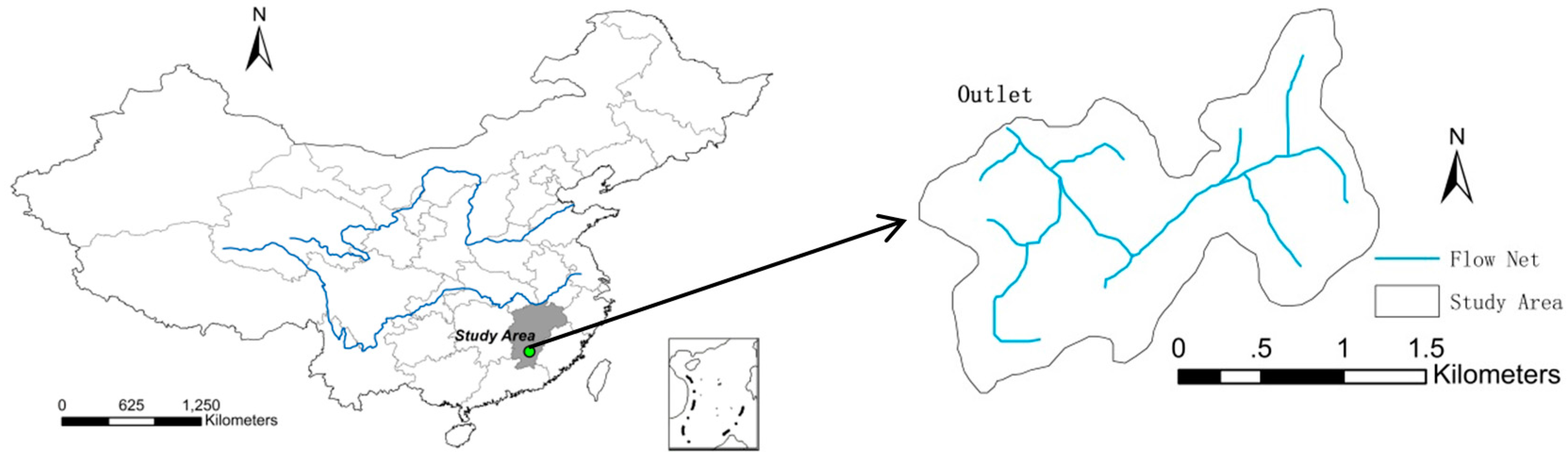
3.1. Study Area

The Zuoma watershed, which is the focus of this study, is located in the southern of Jiangxi Province, China (Figure 1), and has an area of 3.2 km². The watershed area is characterized by hilly topography, with elevation ranging from 119–247 m above sea level. The climate is subtropical monsoon, with an average annual precipitation of 1507 mm. Nearly 47% of annual precipitation occurs during April to June when heavy storms occasionally take place. Red soil is the main soil type of the area, where erosion problems are serious. The major land use depends upon the forest of Masson pine accounting for 77%, the second is farming land that accounts for 12%.

Figure 1. Location of the study watershed in southern of China.

Figure 1. Location of the study watershed in southern of China.

The watershed has the only outlet, and a station was established for monitoring runoff and sediment yield of the watershed in 2010, which is situated in 115°24′09″ E longitude and 25°55′19″ N latitude. A continuous-recording water level stage recorder was used to record streamflow, the water stage was measured every 15 min and then transformed into runoff by means of the calibrated rating curve obtained through periodic flow measurements. While a silt sampler (bottle) was used to record sediment flow: (1) the suspended sediment samples were taken every 15 min during rainfall event; (2) the sample was oven dried at 105 °C for 24 h, and the suspended sediment concentration was calculated using the residue weight and the sample volume; (3) the sediment yield of each rainfall event was calculated from the concentration and runoff value.

3.2. The Model Application

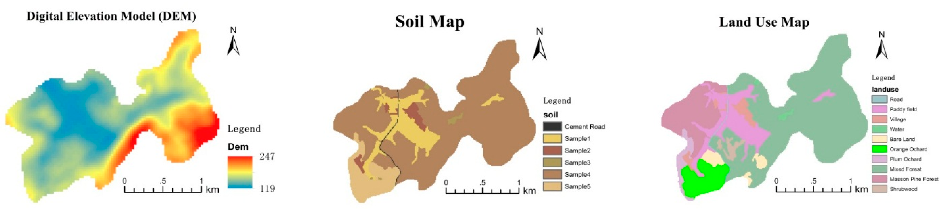
3.2.1. Model Inputs

In this study, the GeoWEPP model requires three graphs including a digital elevation map (DEM), land use map and soil distribution map, all of which are raster files (Figure 2). The DEM is download from Data Sharing Infrastructure of Earth System Science (http://www.geodata.cn/) with 30 m resolution. The land use map is drawn up based on remote sensing image and field interpretation by ArcGIS 10.1. The soil distribution is based on field investigation and analysis results of soil samples which were collected from 20 sites in the watershed (seven were dominated by forest, seven by orchards, three by shrub and three by farm), then the soil was divided into five main types and a cement (road) and mapped by using ArcGIS. All attributes of the three graphs must be consistent.

Figure 2. Three maps needed by GeoWEPP of the study are DEM, soil and land use map.

Figure 2. Three maps needed by GeoWEPP of the study are DEM, soil and land use map.

For predicting soil erosion, it is necessary to supply more data files used by the model, which are soil property file, plant and management file and climate file.

The soil file (.sol) was built through soil file builder within the WEPP interface. Soil basic characteristics, such as percent of sand, silt, clay, organic matter, rock fragment fraction, and cation exchange capacity (CEC) were obtained from the measured data in the study area. Albedo was estimated by Baumer’s formula as suggested in the WEPP model. The initial saturation level was instead of average water content of January. Other soil characteristics, such as the rill and interill erodibility, the critical shear for flow hydraulic, and effective hydraulic conductivity of surface soil were internally calculated by formulas suggested in WEPP [35]. Table 1 shows the mean properties of five soil types in the soil map.

Table 1. Soil properties used for simulation.

Soil Properties	Soil Types
	1	2	3	4	5	Mean
Sand (%)	45.0	52.3	69.5	45.9	53.5	53.2
Clay (%)	30.7	30.2	7.3	33.4	28.2	25.9
Organic matter (%)	0.48	0.36	3.06	1.40	1.84	7.14
CEC (meq/100g)	8.1	7.4	8.5	8.5	6.9	7.9
Rock fragment (%)	15	15	5	10	10	11
Albedo	0.50	0.58	0.176	0.342	0.287	0.377
Initial saturation level (%)	75	75	75	75	75	75

Table 1. Soil properties used for simulation.

Soil Properties	Soil Types
	1	2	3	4	5	Mean
Sand (%)	45.0	52.3	69.5	45.9	53.5	53.2
Clay (%)	30.7	30.2	7.3	33.4	28.2	25.9
Organic matter (%)	0.48	0.36	3.06	1.40	1.84	7.14
CEC (meq/100g)	8.1	7.4	8.5	8.5	6.9	7.9
Rock fragment (%)	15	15	5	10	10	11
Albedo	0.50	0.58	0.176	0.342	0.287	0.377
Initial saturation level (%)	75	75	75	75	75	75

The plant and management parameter file (.rot) includes plant parameters, tillage sequences and tillage implement parameters, plant and residue management, initial conditions, contouring, subsurface drainage and crop rotations. According to land use and the characteristics of local crops combined with mass survey and historical data, ten plant and management parameter files in WEPP were used and some parameters were adjusted to fit measured plant characteristics such as height, cover percentage, or leaf area index cover, and tillage implement parameters.

Finally, the climate file (.cli) was generated by using the CLIGEN model. Firstly, a GDS format file of GANZHOU weather station was downloaded from Agricultural Research Service (http://hydrolab.arsusda.gov/nicks/nicks.htm), which is the nearest international weather station to the study area. Then, a similar US station was searched for using the GDS format file to develop the CLIGEN parameter file. Finally, 1970–2013 daily data was loaded, which includes daily rainfall, the highest temperature and the lowest temperature. The climate file was then produced.

3.2.2. Model Calibration and Validation

Calibration and sensitivity analysis of the model is necessary for assessing the rationality of the model and identifying input parameters [37]. The measured yearly runoff and sediment yield of 2010 and 2012 were used to sensitivity analysis and calibrate, and the measured monthly data of 2011 were used for validation. With the results of previous studies [38,39], the calibration process focused mainly on input parameters included interrill erodibility and effective hydraulic conductivity of soil properties and leaf area index and cover percentage of plant parameters to ensure the absolute errors of simulated values and measured values not more than 15%. All the measured data used in this study are displayed in Table 2.

To evaluate the prediction performances of the model, the basis of test criteria recommended by the ASCE Task Committee [40] and graphical performances criteria suggested by Haan [41] were used. While a group measures include the coefficient of residual mass (CRM), the coefficient of determination (R²), root mean square error (RMSE), Nash–Sutcliffe efficiency (E_NS) [42] and modified Nash–Sutcliffe efficiency (ME_NS) [43] are also used as goodness-of-fit criterions, which can indicate over- or under-prediction for each sample and total value [44]. The descriptions of these measures are shown in Table 3.

Table 2. The measured data from the outlet monitoring station.

Time	Runoff (m3)	Sediment Yield (t)
Yearly data
2010	2,230,000	5500
2011	1,620,000	5190
2012	2,310,000	5510
Monthly data of 2011
January	49,571	25
February	136,821	577
March	128,254	127
April	35,694	21
May	382,977	1273
June	254,093	827
July	199,173	747
August	126,113	253
September	79,821	398
October	185,339	76
November	31,193	170
December	12,508	15

Table 2. The measured data from the outlet monitoring station.

Time	Runoff (m3)	Sediment Yield (t)
Yearly data
2010	2,230,000	5500
2011	1,620,000	5190
2012	2,310,000	5510
Monthly data of 2011
January	49,571	25
February	136,821	577
March	128,254	127
April	35,694	21
May	382,977	1273
June	254,093	827
July	199,173	747
August	126,113	253
September	79,821	398
October	185,339	76
November	31,193	170
December	12,508	15

Table 3. Measures of model performance assessment.

Coefficient or Measure	Equation	Range of Variability	Optimal Value
Coefficient of residual mass	$\text{CRM}=\frac{{\displaystyle {\sum }_{\text{i}=1}^{\text{n}}{Q}_{\text{i}}-{\displaystyle {\sum }_{\text{i}=\text{1}}^{\text{n}}{\text{P}}_{\text{i}}}}}{{\displaystyle {\sum }_{i=1}^n{Q}_i}}$	−∞ to +∞	0
Coefficient of determination	${\text{R}}^{\text{2}}={\left[\frac{{\displaystyle \sum \left(Q_{\text{i}}-\overline{Q}\right)\left({\text{P}}_{\text{i}}-\overline{\text{P}}\right)}}{\sqrt{{\displaystyle \sum {\left({\text{Q}}_{\text{i}}-\overline{Q}\right)}^2•{\displaystyle \sum {\left(P_{\text{i}}-\overline{\text{P}}\right)}^2}}}}\right]}^2$	0 to 1	1
Root mean square error	$RMSE=\sqrt{\frac{{\displaystyle \sum _{\text{i}=1}^n{\left(P_i-Q_i\right)}^2}}{n}}$	0 to ∞	0
Nash–Sutcliffe efficiency	${\text{E}}_{\text{NS}}=1-\frac{{\displaystyle {\sum }_{\text{i}=1}^{\text{n}}{\left({\text{Q}}_{\text{i}}-P_i\right)}^2}}{{\displaystyle {\sum }_{i=1}^n{\left(Q_i-\overline{Q}\right)}^2}}$	−∞ to 1	1
Modified Nash–Sutcliffe efficiency	${\text{ME}}_{\text{NS}}=1-\frac{{\displaystyle {\sum }_{\text{i}=1}^{\text{n}}\left|Q_i-P_i\right|}}{{\displaystyle {\sum }_{i=1}^n\left|Q_i-\overline{Q}\right|}}$	−∞ to 1	1

n = number of observations; $Q_i$, $P_{\text{i}}$ = measured and simulated value at i; $\overline{Q}$, $\overline{P}$ = average measured and simulated value.

Table 3. Measures of model performance assessment.

Coefficient or Measure	Equation	Range of Variability	Optimal Value
Coefficient of residual mass	$\text{CRM}=\frac{{\displaystyle {\sum }_{\text{i}=1}^{\text{n}}{Q}_{\text{i}}-{\displaystyle {\sum }_{\text{i}=\text{1}}^{\text{n}}{\text{P}}_{\text{i}}}}}{{\displaystyle {\sum }_{i=1}^n{Q}_i}}$	−∞ to +∞	0
Coefficient of determination	${\text{R}}^{\text{2}}={\left[\frac{{\displaystyle \sum \left(Q_{\text{i}}-\overline{Q}\right)\left({\text{P}}_{\text{i}}-\overline{\text{P}}\right)}}{\sqrt{{\displaystyle \sum {\left({\text{Q}}_{\text{i}}-\overline{Q}\right)}^2•{\displaystyle \sum {\left(P_{\text{i}}-\overline{\text{P}}\right)}^2}}}}\right]}^2$	0 to 1	1
Root mean square error	$RMSE=\sqrt{\frac{{\displaystyle \sum _{\text{i}=1}^n{\left(P_i-Q_i\right)}^2}}{n}}$	0 to ∞	0
Nash–Sutcliffe efficiency	${\text{E}}_{\text{NS}}=1-\frac{{\displaystyle {\sum }_{\text{i}=1}^{\text{n}}{\left({\text{Q}}_{\text{i}}-P_i\right)}^2}}{{\displaystyle {\sum }_{i=1}^n{\left(Q_i-\overline{Q}\right)}^2}}$	−∞ to 1	1
Modified Nash–Sutcliffe efficiency	${\text{ME}}_{\text{NS}}=1-\frac{{\displaystyle {\sum }_{\text{i}=1}^{\text{n}}\left|Q_i-P_i\right|}}{{\displaystyle {\sum }_{i=1}^n\left|Q_i-\overline{Q}\right|}}$	−∞ to 1	1

n = number of observations; $Q_i$, $P_{\text{i}}$ = measured and simulated value at i; $\overline{Q}$, $\overline{P}$ = average measured and simulated value.

3.3. Scenarios Analysis for Simulation

To understand the effects of different land use on soil erosion in the red soil region, the GeoWEPP model was run for the following four theoretic scenarios of the study watershed, which are under a single land use type:

• S1 (scenario1): forest land
• S2 (scenario2): farm land
• S3 (scenario3): orchard land
• S4 (scenario4): fallow land

All of the land use types are typical and generally applicable in the watershed and other regions of the red soil. For controlling the influence of soil distribution, the mean volume of soil properties (Table 1) was used as the soil input parameters of the whole watershed for all simulation scenarios.

Combining slope gradient map and erosion distribution map of the four scenarios in which the erosion were divided into several classes according to the range of sediment yield, using the ArcGIS 10.1 analysis tool, the average sediment yield under different slope gradient were calculated by following equation:

$${\text{Sed}}_{{\text{g}}_{\text{k}}}=\frac{{\displaystyle {\sum }_{i=1}^n{s}_{i\text{k}}{y}_{i\text{k}}}}{{\displaystyle {\sum }_{i=1}^n{s}_{i\text{k}}}}$$

(1)

where $g_k$ is the slope gradient of k value, $Se{d}_{g_k}$ is the average sediment yield under $\text{k}$ slope gradient, ${\text{s}}_{\text{ik}}$ and ${\text{y}}_{\text{i}k}$ are respectively the area and the middle value of the $\text{i}$ erosion class of $\text{k}$ slope gradient, $\text{n}$ is the number of divided erosion class for different land use.

4. Results and Discussion

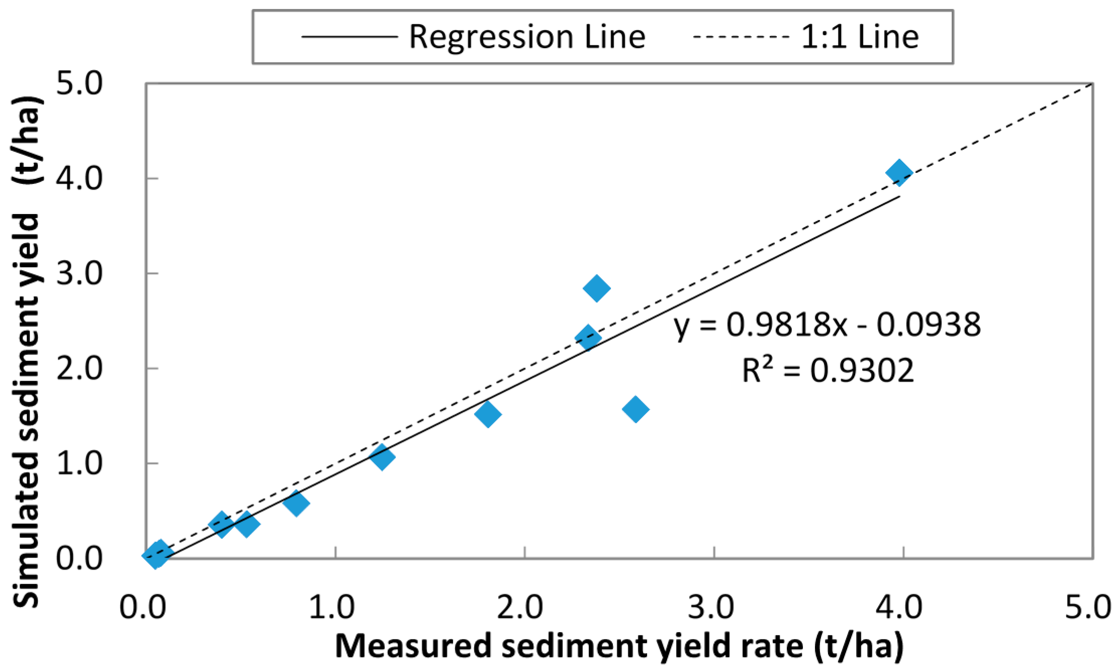
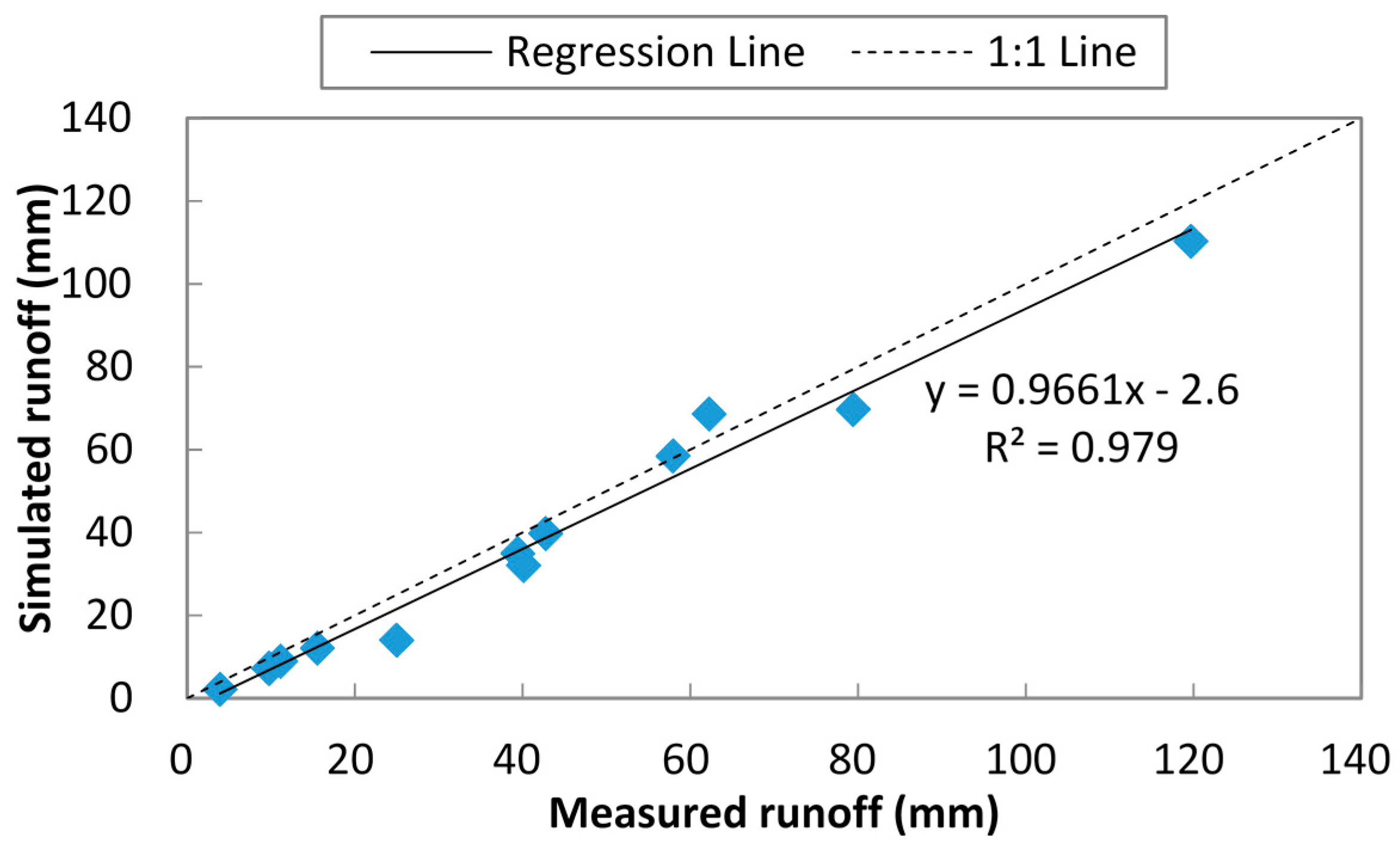
4.1. Performance of the GeoWEPP Model

This study aims to simulate the runoff and sediment yield for four typical land uses of the watershed and analyze the effects of slope gradient by the GeoWEPP model. Thus, the performance of the model is very important to the results of following analysis. After proper calibration, the model was evaluated for the simulation of runoff and sediment yield using the 2011 monthly measured data. The measured and simulated monthly runoff and sediment yield for validation along with 1:1 line are shown in Figure 3 and Figure 4, respectively. It is observed from Figure 3 that simulated runoff values are distributed uniformly along the1:1 line. While the simulated sediment yields are found to be distributed uniformly along the 1:1 line (Figure 4) except at two different points, of which one simulated value is higher than measured value and the other is lower.

Figure 3. Validated measured and simulated monthly runoff for 2011.

Figure 3. Validated measured and simulated monthly runoff for 2011.

Figure 4. Validated measured and simulated monthly sediment yield for 2011.

Figure 4. Validated measured and simulated monthly sediment yield for 2011.

Goodness-of-fit statistics for simulation of monthly runoff and sediment yield are shown in Table 4. The higher the coefficient of determination values of 0.98 and 0.93 respectively for runoff and sediment yield indicate a close relationship between the measured and simulated values. It is seen from Table 4 that the maximum value of runoff is slightly lower, which results in slightly lower standard deviation and mean for the simulated value, when the slightly higher maximum value results in higher standard deviation with lower total value for the simulated sediment yield. However, the means of simulation of monthly runoff and sediment yield are not significantly different at 95% confidence level as t-calculated < t-critical. High E_NS values of 0.96 and 0.91 and ME_NS values (0.86, 0.93) and low RSME values (6.91mm, 0.35 t∙ha⁻¹) both for runoff and sediment yield indicated that the model can be well adopted for simulation of runoff and sediment. The good performance of the model is similar to other studies. Yu et al. [27], for example, used the model to simulate multi-scale watershed runoff and sediment production in China, and the simulation results present satisfactory performance with the relative errors of simulated values of runoff and sediment yield are below 30%, the correlation coefficients are above 0.90, and the Nash-Suttcliffe efficiency coefficients are above 0.80, Yuksel et al. [45] also found the GeoWEPP model could provide good results in predicting runoff and sediment yield from Orcan Creek watershed in Kahramanmaras region, which had simple land use distribution as our study area: the Zuoma watershed.

Table 4. Statistical analysis of observed and simulated monthly runoff and sediment yield, 2011.

Statistical Parameter	Runoff (mm)		Sediment Yield (t/ha)
	Measured	Simulated	Measured	Simulated
Mean	42.23	38.20	1.35	1.23
Standard deviation	33.77	32.97	1.26	1.28
Maximum	119.68	110.28	3.98	4.06
Total	506.74	458.37	16.24	14.82
CRM	0.095		0.087
R2	0.98		0.93
ENS	0.96		0.91
MENS	0.86		0.93
RMSE	6.19		0.35
t-calculated at 95% confidence level	0.39		0.41
t-critical (two tail)	0.77		0.82

Table 4. Statistical analysis of observed and simulated monthly runoff and sediment yield, 2011.

Statistical Parameter	Runoff (mm)		Sediment Yield (t/ha)
	Measured	Simulated	Measured	Simulated
Mean	42.23	38.20	1.35	1.23
Standard deviation	33.77	32.97	1.26	1.28
Maximum	119.68	110.28	3.98	4.06
Total	506.74	458.37	16.24	14.82
CRM	0.095		0.087
R2	0.98		0.93
ENS	0.96		0.91
MENS	0.86		0.93
RMSE	6.19		0.35
t-calculated at 95% confidence level	0.39		0.41
t-critical (two tail)	0.77		0.82

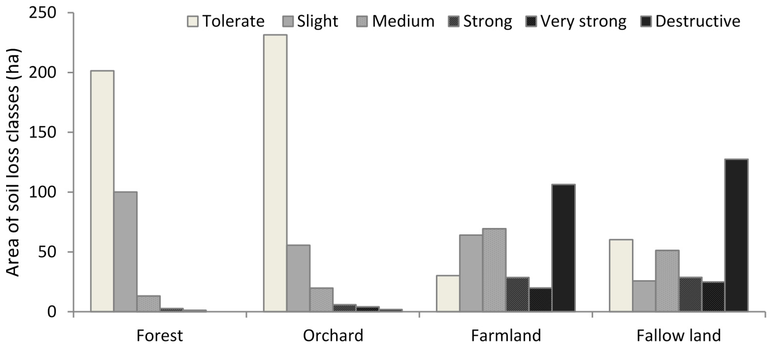
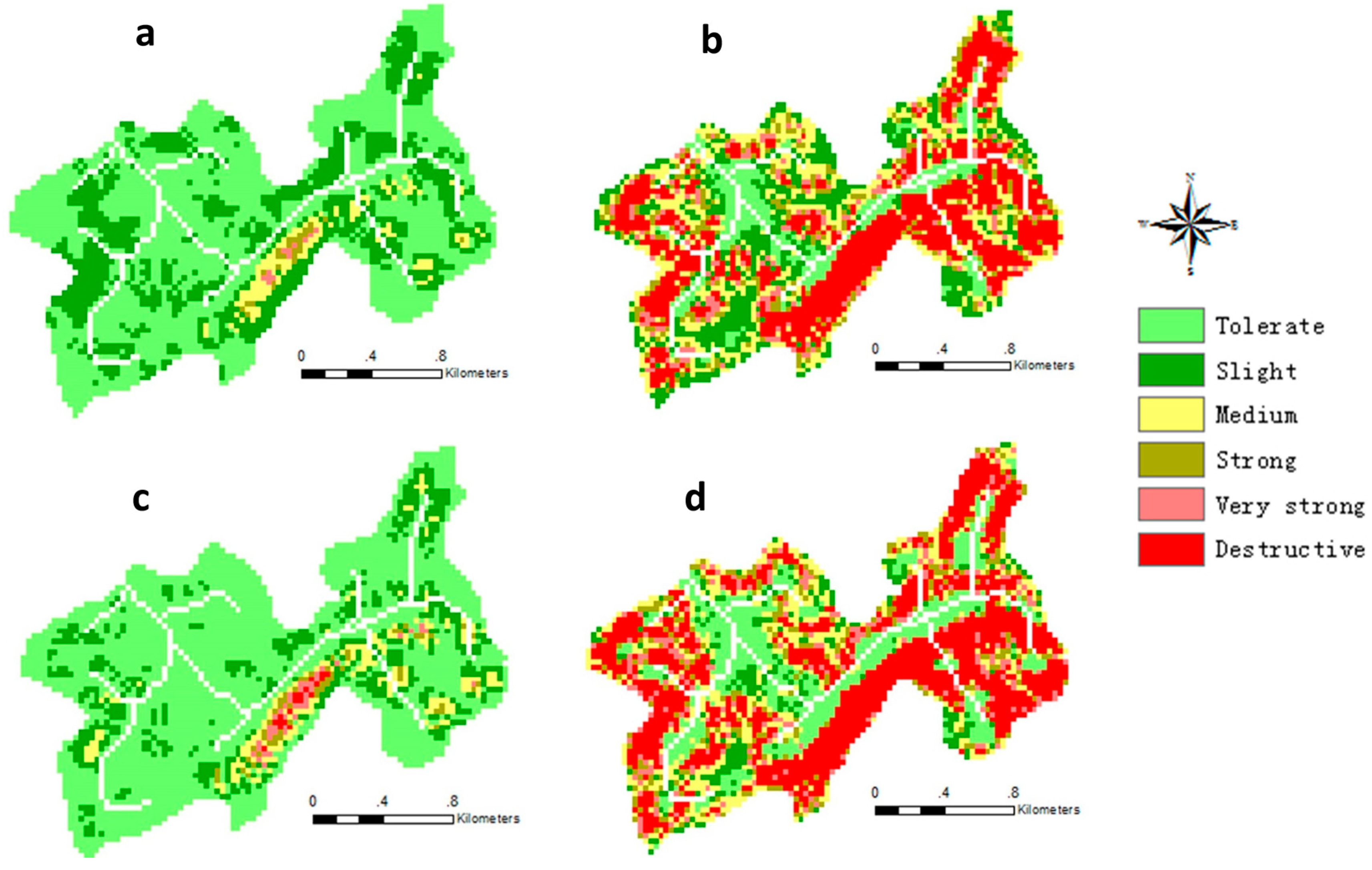
4.2. Effects of Land Use and Slope Gradient on Soil Erosion

There are serious soil erosion problems in the red soil region. One of the reasons is the lack of adequate land use planning which can accelerate water soil erosion and create major environmental problems. The GeoWEPP model here was run for four scenarios with typical land use under the same soil type and climate in the Zuoma watershed. The results were shown in Table 5.

Table 5. Results of simulation for the four scenarios.

Result Description	Scenarios
	CLU	Forest	S2 Farmland	Orchard	Fallow
Mean annual runoff (m^3)	2,053,548	1,135,527	3,123,356	800,594	2,995,423
Mean annual runoff depth (mm)	642	355	976	250	936
Change in runoff as compared to CLU (%)	-	−44.70	52.02	−61.06	45.8
Mean annual sediment yield (t)	5400	3042	7714	1692	7006
Mean annual Sed. rate (t∙ha−1)	16.9	9.5	24.1	5.3	21.9
Change in sediment yield as compared to CLU (%)	-	−43.67	42.6	−68.64	29.6

CLU presents current land use; “−” presents reduction.

Table 5. Results of simulation for the four scenarios.

Result Description	Scenarios
	CLU	Forest	S2 Farmland	Orchard	Fallow
Mean annual runoff (m^3)	2,053,548	1,135,527	3,123,356	800,594	2,995,423
Mean annual runoff depth (mm)	642	355	976	250	936
Change in runoff as compared to CLU (%)	-	−44.70	52.02	−61.06	45.8
Mean annual sediment yield (t)	5400	3042	7714	1692	7006
Mean annual Sed. rate (t∙ha−1)	16.9	9.5	24.1	5.3	21.9
Change in sediment yield as compared to CLU (%)	-	−43.67	42.6	−68.64	29.6

CLU presents current land use; “−” presents reduction.

Table 5 depicts runoff and sediment yield varying with land use types but have the same trend. The highest predicted mean annual runoff depth (976 mm) and sediment yield rate (24.1 t∙ha⁻¹) occurs in the farm land (scenario 2) and the lowest runoff depth (250 mm) and sediment yield rate (5.3 t∙ha⁻¹) in the orchard land (scenario 3), while mean annual runoff depth and sediment yield rate from the watershed for the forest land (scenario 1) and the fallow land (scenario 4) are 355 mm and 936 mm, and 9.5 t∙ha⁻¹ and 21.9 t∙ha⁻¹, respectively. Comparing with current land use (CLU) of the watershed, the forest and orchard land show positive effects on reducing runoff and sediment yield while the farmland and fallow land have opposite effects.

4.2.1. Runoff and Sediment Yield in Response to Land Use Change

The sediment yield of the four theoretical scenarios are separated into six classes in Figure 5a–d: (a) tolerate (<5 t∙ha⁻¹∙year⁻¹); (b) slight (5 to 15 t∙ha⁻¹∙year⁻¹); (c) medium (15 to 40 t∙ha⁻¹∙year⁻¹); (d) strong (40 to 60 t∙ha⁻¹∙year⁻¹); (e) very strong (60 to 80 t∙ha⁻¹∙year⁻¹); and (f) destructive (>80 t∙ha⁻¹∙year⁻¹). These classifications were referred to “Technical standards for comprehensive control of water and soil erosion in the red soil hilly region in southern China (SL657-2014)”, in which 5 t∙ha⁻¹∙year⁻¹ is an appropriate boundary value for soil loss in the red soil hilly region.

Figure 5. Sediment yield maps of the Zuoma watershed for S1 (a); S2 (b); S3 (c); and S4 (d).

Figure 5. Sediment yield maps of the Zuoma watershed for S1 (a); S2 (b); S3 (c); and S4 (d).

Figure 6 shows the areas of different soil loss classes for the four scenarios. It is seen from Figure 6 that the soil loss area of forest land and orchard land are reduced along with the increase of the erosion degree. The highest area and percentage in tolerate category are 201.4 ha and 63.21%, and 231.4 ha and 72.63%, respectively for forest land and orchard land, both of which are more than half. The area (106.4 ha accounted for 33.40%) of the destructive category is highest for farmland while the slight category (64.0 ha) and medium category (69.4 ha) account for larger portions. The areas of tolerate to destructive categories are 60.2 ha, 25.8 ha, 51.3 ha, 28.8 ha, 25.0 ha and 127.5 ha for fallow land, in which the destructive category is also with the highest area percentage.

Figure 6. Area of different soil loss classes for the four land use.

Figure 6. Area of different soil loss classes for the four land use.

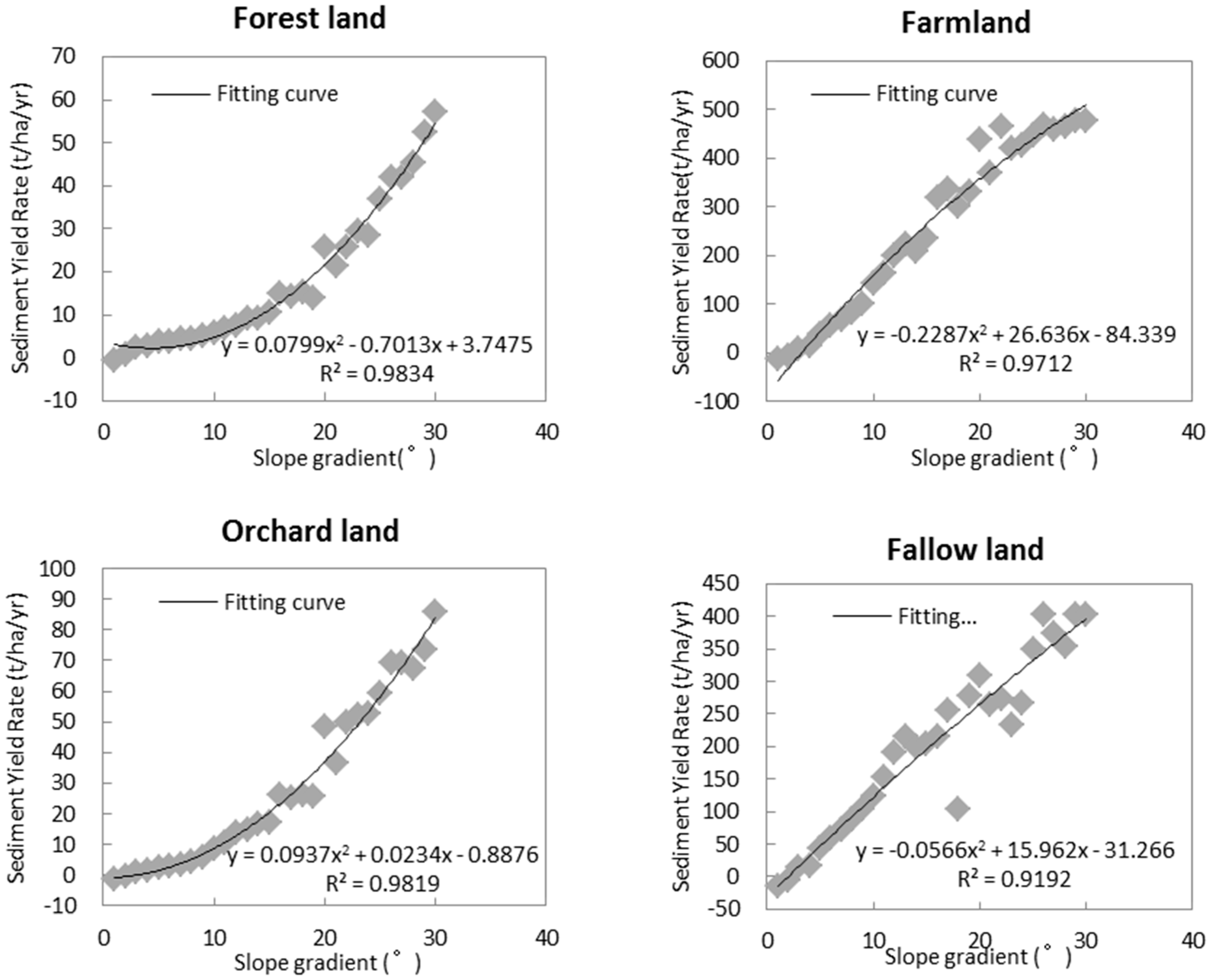
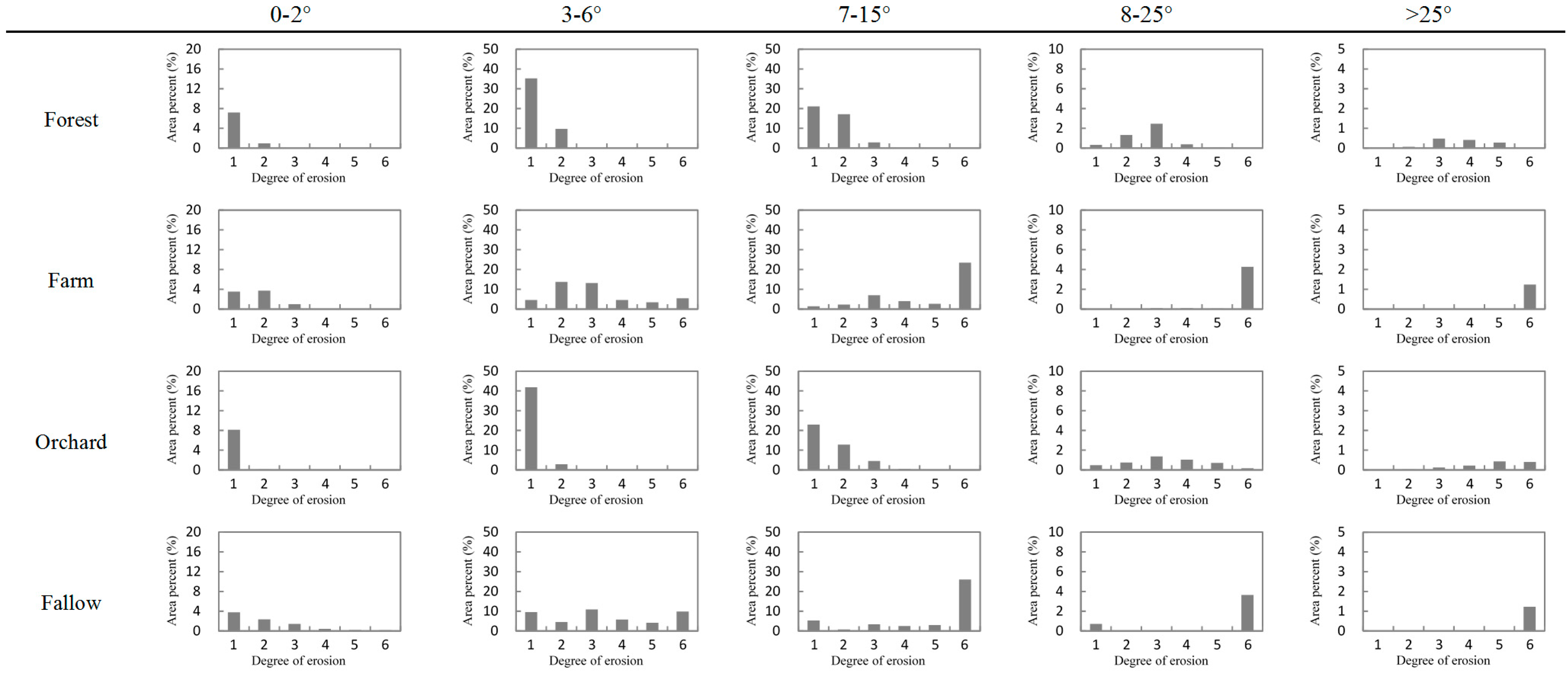
4.2.2. Soil Erosion and Slope Gradient

Figure 7 shows the interaction of land use, slope gradient and soil erosion. The slope gradient is divided into five classes, 0°–2°, 3°–6°, 7°–15°, 16°–25° and >25°, respectively which represents flat, slowly, oblique, steep and very steep slope condition. The area percentage (compared to the area of the Zuoma watershed) of each erosion degree under different slope class is graphed by histograms. It is seen from Figure 7 that the erosion degree with the highest area percentage values under forest land are tolerate erosion for slope class 1, 2 and 3 and medium erosion for slope class 4 and 5, as similar as performance showed under orchard land. While the erosion degrees of the highest area percentage values are slight, medium, destructive, destructive and destructive respectively for slope class 1 to 5 under farmland and fallow land. These results indicate that soil erosion is bound up with slope gradient, and the main erosion degree increases with the slope gradient increasing under all land use types.

Figure 7. The interaction of soil erosion, slope gradient and land use. The numbers of 1–6 (degree of erosion) respectively presents Tolerate to Destructive erosion categories.

Figure 7. The interaction of soil erosion, slope gradient and land use. The numbers of 1–6 (degree of erosion) respectively presents Tolerate to Destructive erosion categories.

Based on the method as previously described, the relationships between slope gradient and soil erosion rate of different scenarios or land use types were established (Figure 8). From Figure 8, it can be seen that the erosion rate increase by quadratic regression in the study watershed. In a study by Smith and Wischmeier [46], the relationship between soil erosion and slope of the two degree polynomial was put forward using field plot measured with slope of 3%, 8%, 13% and 18% which was applied to the first edition of Universal Soil Loss Equation (USLE). Other researchers found that the soil erosion increased exponentially with increasing slope gradient [11] but the relationships were different for different slope conditions, landforms, soil types and other factors [47,48].

Figure 8. Relationship between soil erosion and slope gradient.

Figure 8. Relationship between soil erosion and slope gradient.

According to the equations shown in Figure 8, the soil erosion for the forest, orchard, farm land and fallow land at slope gradient of 15°, the lowest criteria slope gradient to determine whether farmland should be changed in the “Grain-to-Green” Program, is 11 t∙ha⁻¹∙year⁻¹, 264 t∙ha⁻¹∙year⁻¹, 21 t∙ha⁻¹∙year⁻¹ and 220 t∙ha⁻¹∙year⁻¹ respectively, which intuitively shows that the farmland at the gradient of over 15° must be returned to forest and grass as well as the fallow land, but the value of 15° as the criteria slope gradient to control soil erosion in this study area is totally unreasonable. According to the standard of soil conservation in the red soil hilly region in southern China, for soil erosion not more than the medium amount of erosion (15–40 t∙ha⁻¹∙year⁻¹), the slope gradient of tolerate areas for forest, orchard, farmland and fallow land should be less than 28°, 21°, 5° and 5° respectively, which provides a simple and intuitive manner for land use planning to control soil erosion. The relationship of slope gradient and erosion under orchard land also indicates that the farmland and fallow land can not only be changed to forest but also to orchard in this study area or similar areas, which can increase economic benefits compared with forest or grass land. In addition, the equations also can be used to predict soil erosion by analyzing land use and slope gradient distributions in similar regions.

5. Conclusions

A soil erosion model, GeoWEPP, was used to predict runoff and sediment yield from a small watershed of red soil in southern China, and four scenarios of typical land use types were simulated by the model to evaluate the effects of land use on soil erosion. The results obtained through this study show that:

(1)

The GeoWEPP model had good performance in the study area with higher accuracy in sediment yield than in runoff predictions and provided a simple method for making decisions of selecting soil conservation practices when combined with scenario analysis.

(2)

The order of land use by increasing sediment yield was: farm land > fallow land > orchard land > forest land, with 42.6% > 29.6% > −43.07% > −68.04% as compared to the average annual sediment yield under the current land use. It indicated that farm land was the most important element for contributing to soil erosion, even beyond fallow land. Therefore, appropriate land use planning was important for soil conservation of a watershed.

(3)

The soil erosion increased with increasing slope gradient under all scenarios, and quadratic equations describing the relationships were reliable for all land use. These equations could not only be used to decide the critical slope gradient of farm, fallow and orchard land turning to forest but also to predict the sediment yield of these typical land use under different slope conditions in the study area and other similar regions.

References

1. Flanagan, D. Erosion Encyclopedia of Soil Science, 1st ed.; Marcel Dekker: New York, NY, USA, 2002; pp. 395–398. [Google Scholar]
2. Kosmas, C.; Danalatos, N.; Cammeraat, L.H.; Chabart, M.; Diamantopoulos, J.; Farand, R. The effect of land use on runoff and soil erosion rates under Mediterranean conditions. Catena 1997, 29, 45–59. [Google Scholar] [CrossRef]
3. Braud, I.; Vich, A.I.J.; Zuluaga, J.; Fomero, L.; Pedrani, A. Vegetation influenceon runoff and sediment yield in the Andes Region: Observation and modeling. J. Hydrol. 2001, 254, 124–144. [Google Scholar] [CrossRef]
4. Fiener, P.; Auerswald, K.; van Oost, K. Spatio-temporal patterns in land use and management affecting stremflow response of agricultural catchments-a review. Earth Sci. Rev. 2011, 106, 92–104. [Google Scholar] [CrossRef]
5. Ewert, F.; Rounsevell, M.D.A.; Reginster, I.; Metzger, M.J.; Leemans, R. Future scenarios of European agricultural land use I. Estimating changes in crop productivity. Agric. Ecosyst. Environ. 2005, 107, 101–116. [Google Scholar] [CrossRef]
6. Bakker, M.M.; Govers, G.; van Doom, A.; Quetier, F.; Chouvardas, D.; Rounsevell, M. The response of soil erosion and sediment export to land-use change in four areas of Europe: The importance of landscape pattern. Geomorphology 2008, 98, 213–226. [Google Scholar] [CrossRef]
7. Feng, X.; Wang, Y.; Chen, L.; Fu, B.; Bai, G. Modeling soil erosion and its response to land-use change in hilly catchments of the Chinese Loess Plateau. Geomorphology 2010, 118, 239–248. [Google Scholar] [CrossRef]
8. Fu, B.J.; Wang, Y.F.; Lu, Y.H.; He, C.S.; Chen, L.D.; Song, C.J. The effects of landuse combinations on soil erosion: A case study in the Loess Plateau of China. Prog. Phys. Geogr. 2009, 33, 793–804. [Google Scholar] [CrossRef]
9. Shi, Z.H.; Ai, L.; Fang, N.F.; Zhu, H.D. Modeling the impacts of integrated small watershed management on soil erosion and sediment delivery: A case study in the Three Gorges Area, China. J. Hydrol. 2012, 438, 156–167. [Google Scholar] [CrossRef]
10. Deng, L.; Shangguan, Z.-P.; Li, R. Effects of the grain-for-green program on soil erosion in China. Int. J. Sediment. Res. 2012, 27, 120–127. [Google Scholar] [CrossRef]
11. Jordan, G.; van Rompaey, A.; Szilassi, P.; Csillag, G.; Mannaerts, C.; Woldai, T. Historical land use changes and their impact on sediment fluxes in the Balaton basin (Hungary). Agric. Ecosyst. Environ. 2005, 108, 119–133. [Google Scholar] [CrossRef]
12. Shi, L.R. Hillside field improvement of Yangtze valley. Yangtze River 1999, 30, 25–27. (In Chinese) [Google Scholar]
13. Li, M.A.; Yao, W.Y.; Li, Z.B.; Liu, P.L.; Shen, Z.Z. Effects of landforms on the erosion rate in a small watershed by the Cs-137 tracing method. J. Environ. Radioact. 2010, 101, 380–384. [Google Scholar] [CrossRef] [PubMed]
14. Zingg, A.W. Degree and length of land slope as it affects soil loss in runoff. Agric. Eng. 1940, 21, 59–64. [Google Scholar]
15. Smith, D.D.; Wischmeier, W.H. Factors affecting sheet and rill erosion. Am. Geophys. Union Trans. 1958, 38, 889–896. [Google Scholar] [CrossRef]
16. Chaplot, V.A.M.; le Bissonnais, Y. Runoff features for interrill erosion at different rainfall intensities, slope lengths, and gradients in an agricultural loessial hillslope. Soil Sci. Soc. Am. J. 2003, 67, 844–851. [Google Scholar] [CrossRef]
17. Assouline, S.; Ben-Hur, A. Effects of rainfall intensity and slope gradient on the dynamics of interrill erosion during soil surface sealing. Catena 2006, 66, 211–220. [Google Scholar] [CrossRef]
18. Zhao, X.N.; Huang, J.; Wu, P.T.; Gao, X.D. The dynamic effects of pastures and crop on runoff and sediments reduction at loess slopes under simulated rainfall conditions. Catena 2014, 119, 1–7. [Google Scholar] [CrossRef]
19. Huang, M.B.; Gallichand, J.; Wang, Z.L.; Goulet, M. A modification to the Soil Conservation Service curve number method for steep slopes in the Loess Plateau of China. Hydrol. Process. 2006, 20, 579–589. [Google Scholar] [CrossRef]
20. Liu, B.Y.; Nearing, M.A.; Risse, L.M. Slope gradient effects on soil loss for steep slopes. Trans. Am. Soc. Agric. Eng. 1994, 37, 1835–1840. [Google Scholar] [CrossRef]
21. Jiang, F.S.; Huang, Y.H.; Wang, M.K.; Lin, J.S.; Zhao, G.; Ge, H.L. Effects of Rainfall Intensity and Slope Gradient on Steep Colluvial Deposit Erosion in Southeast China. Soil Sci. Soc. Am. J. 2014, 78, 1741–1752. [Google Scholar] [CrossRef]
22. Li, M.; Li, Z.B.; Yao, W.Y. Estimating the erosion and deposition rates in a small watershed by the 137Cs tracing method. Appl. Radiat. Isot. 2009, 67, 362–366. [Google Scholar] [CrossRef] [PubMed]
23. Stolt, M.H.; Baker, J.C.; Simpson, T.W. Soil-landscape relationships in Virginia: II. Reconstruction analysis and soil genesis. Soil Sci. Soc. Am. J. 1993, 57, 422–428. [Google Scholar] [CrossRef]
24. Tang, K.L.; Zhang, K.L.; Lei, A.L. Critical slope gradient for compulsory abandonment of farmland on the hilly Loess Plateau. Chin. Sci. Bull. 1998, 43, 409–412. [Google Scholar] [CrossRef]
25. Flanagan, D.C.; Frankenberger, J.R.; Renschler, C.S.; Laflen, J.M.; Engel, B.A. Simulating small watersheds with Water Erosion Prediction Project technology. In Proceedings of the Soil Erosion Research for the 21st Century, Honolulu, HA, USA, 3–5 January 2001; Ascough II, J.C., Flanagan, D.C., Eds.; American Society of Agricultural Engineers: St. Joseph, MI, USA, 2001; pp. 363–366. [Google Scholar]
26. Renschler, C.S. Designing geo-spatial interfaces to scale process models: The GeoWEPP approach. Hydrol. Process. 2003, 17, 1005–1017. [Google Scholar] [CrossRef]
27. Yu, X.; Zhang, X.; Niu, L. Simulated multi-scale watershed runoff and sediment production based on GeoWEPP model. Int. J. Sediment. Res. 2009, 24, 465–478. [Google Scholar] [CrossRef]
28. Maalim, F.K.; Melesse, A.M.; Belmont, P.; Gran, K.B. Modeling the impact of land use changes on runoff and sediment yield in the Le Sueur watershed, Minnesota using GeoWEPP. Catena 2013, 107, 35–45. [Google Scholar] [CrossRef]
29. Wang, X.D.; Jiang, Y.Z.; Zhao, H.L.; Liang, Y.Q. The application of distributional hydrological model of water resources management to river basins. South-to-North Water Transf. Water Sci. Technol. 2004, 2, 4–7. (In Chinese) [Google Scholar]
30. Raclot, D.; Albergel, J. Runoff and water erosion modelling using WEPP on a Mediterranean cultivated catchment. Phys. Chem. Earth 2006, 31, 1038–1047. [Google Scholar] [CrossRef]
31. Moore, A.D.; McLaughlin, R.A.; Mitasova, H.; Line, D.E. Calibrating WEPP model parameters for erosion prediction on construction sites. Trans. Asabe 2007, 50, 507–516. [Google Scholar] [CrossRef]
32. Yadav, V.; Malanson, G.P. Modeling impacts of erosion and deposition on soil organic carbon in the Big Creek Basin of southern Illinois. Geomorphology 2009, 106, 304–314. [Google Scholar] [CrossRef]
33. Miller, M.E.; MacDonald, L.H.; Robichaud, P.R.; Elliot, W.J. Predicting post-fire hillslope erosion in forest lands of the western United States. Int. J. Wildland Fire 2011, 20, 982–999. [Google Scholar] [CrossRef]
34. Flanagan, D.C.; Nearing, M.A. USDA Water Erosion Prediction Project: Hillslope Profile and Watershed Model Documentation, 2nd ed.; USDA-ARSNSERL Report 10; USDA-ARS National Soil Erosion Research Laboratory: West Lafayette, IN, USA, 1995. [Google Scholar]
35. Nicks, A.D.; Lane, L.J.; Gander, G.A. Weather generator. In USDA-Water Erosion Prediction Project: Hillslope PRofile and Watershed Model Documentation, 2nd ed.; Flanagan, D.C., Nearing, M.A., Eds.; NSERL Report 10; USDA-ARS National Soil Erosion Research Laboratory: West Lafayette, IN, USA, 1995. [Google Scholar]
36. Lal, R. Soil Erosion Research Methods, 3rd ed.; Soil and Water Conservation Association: Ankeny, IA, USA, 1988; p. 244. [Google Scholar]
37. Nearing, M.A.; Deer-Ascough, L.; Laflen, J.M. Sensitivity analysis of the WEPP Hillslope profile erosion model. Trans. ASAE 1990, 33, 839–849. [Google Scholar] [CrossRef]
38. Bhuyana, S.J.; Kalita, P.K.; Janssenc, K.A.; Barnesa, P.L. Soil loss predictions with three erosion simulation models. Environ. Model. Software 2002, 17, 135–144. [Google Scholar]
39. Pandey, A.; Chowdary, V.M.; Mal, B.C.; Billib, M. Runoff and sediment yield modeling from a small agricultural watershed in India using the WEPP model. J. Hydrol. 2008, 348, 305–319. [Google Scholar] [CrossRef]
40. ASCE Task Committee. Criteria for evaluation of watershed models. J. Irrig. Drain. Eng. 1993, 119, 429–442. [Google Scholar]
41. Haan, C.T.; Johnson, H.P.; Brakensiek, D.L. Hydrological Modeling of Small Watersheds, 4th ed.; American Society of Agricultural Engineers: St. Joseph, MI, USA, 1982. [Google Scholar]
42. Bingner, R.L.; Murphee, C.E.; Mutchler, C.K. Comparison of sediment yield models on various watershed in Mississippi. Trans. ASAE 1989, 32, 529–534. [Google Scholar] [CrossRef]
43. Nash, J.E.; Sutcliffe, J.V. River flow forecasting through conceptual models Part 1-A discussion of principals. J. Hydrol. 1970, 10, 282–290. [Google Scholar] [CrossRef]
44. Zema, D.A.; Bingner, R.L.; Govers, G.; Licciardello, F.; Denisi, P.; Zimbone, S.M. Evaluation of runoff, peak flow and sediment yield for events simulated by the AnnAGNPS model in a Belgian agricultural watershed. Land Degrad. Dev. (Wiley Intersci.) 2012, 23, 205–215. [Google Scholar] [CrossRef]
45. Yuksel, A.; Akay, A.E.; Gundogan, R.; Reis, M.; Cetiner, M. Application of GeoWEPP for determining sediment yield and runoff in the Orcan Creek watershed in Kahramanmaras, Turkey. Sensors 2008, 8, 1222–1236. [Google Scholar] [CrossRef]
46. Smith, D.D.; Wischmeier, W.H. Factors affecting sheet and rill erosion. Trans. Amer. Geophys. Union 1957, 38, 889–896. [Google Scholar] [CrossRef]
47. Foster, G.R. Modeling the erosion process. In Hydrologic Modeling of Small Watersheds; ASAE: St. Joseph, MI, USA, 1982. [Google Scholar]
48. McCool, D.K.; Brown, L.C.; Foster, G.R. Revised slope steepness factor for the Universal Soil Loss Equation. Trans. ASAE 1987, 30, 1387–1396. [Google Scholar] [CrossRef]