Article

A Linear Model for the Estimation of Fuel Consumption and the Impact Evaluation of Advanced Driving Assistance Systems

Department of Civil, Architectural and Environmental Engineering, University of Naples Federico II, via Claudio 21, 80125 Naples, Italy
*
Author to whom correspondence should be addressed.
Sustainability 2015, 7(10), 14326-14343; https://doi.org/10.3390/su71014326
Submission received: 3 August 2015 / Revised: 7 October 2015 / Accepted: 16 October 2015 / Published: 22 October 2015

Abstract

:
Reduction of the environmental impact of cars represents one of the biggest transport industry challenges. Beyond more efficient engines, a promising approach is to use eco-driving technologies that help drivers achieve lower fuel consumption and emission levels. In this study, a real-time microscopic fuel consumption model was developed. It was designed to be integrated into simulation platforms for the design and testing of Advanced Driving Assistance Systems (ADAS), aimed at keeping the vehicle within the environmentally friendly driving zone and hence reducing harmful exhaust gases. To allow integration in platforms employed at early stages of ADAS development and testing, the model was kept very simple and dependent on a few easily computable variables. To show the feasibility of the identification of the model (and to validate it), a large experiment involving more than 100 drivers and about 8000 km of driving was carried out using an instrumented vehicle. An instantaneous model was identified based on vehicle speed, acceleration level and gas pedal excursion, applicable in an extra-urban traffic context. Both instantaneous and aggregate validation was performed and the model was shown to estimate vehicle fuel consumption consistently with in-field instantaneous measurements. Very accurate estimations were also shown for the aggregate consumption of each driving session.

1. Introduction

The research presented here takes place in the framework of traffic behavior studies and the design of Advanced Driving Assistance Systems (ADAS). ADAS are developed by using electronic control units (ECUs) that are designed to supervise the safety, the comfort and the efficiency of the driving. Their design is carried out in the framework of the so-called automotive V-Cycle. In its basic architecture, this process is comprised of a first phase (MIL—model in the loop) of conception of the control logic characteristics and mechanisms, a second phase (SIL—software in the loop) in which the software needed to manage such a logic is developed, and a third phase (HIL—hardware in the loop) consisting of the implementation of the ECU and the evaluation of its interaction with other, actually available, components of the vehicle (hardware sensors, actuators and other devices, and control units).
The research described here falls into the MIL context and is aimed at giving existing ADAS testing platforms the possibility of including an additional module aimed at the simulation of fuel consumption, and thus at testing ADAS oriented to eco-driving solutions. The module is based on a simple model that is able to estimate fuel consumption on the basis of variables that are both easily accessible on vehicles (e.g., readable from the on-board diagnostic—OBD—port with simple after-market solutions) and already available in common modules of vehicle simulation, as implemented in commercial testing platforms (e.g., the software Prescan [1]).
The development and testing of this model is the main focus of this paper. It is based on data collected in two different experiments. The principal experiment concerned driving sessions that took place in the National Research Project DRIVE IN2 (DRIVEr monitoring: technologies, methodologies, and IN-vehicle INnovative systems; [2]), and its data were used for the estimation of the parameters of the model. At a later stage, data of a validation experiment were exploited in order to check the transferability of the model to different contexts.
The paper is organized as follows: Section 2 reviews the literature with respect to the various approaches used for the analysis of fuel consumption; in Section 3 our experiment, tools and collected data are presented; in Section 4 and Section 5, some models are presented and discussed; finally in Section 6 some conclusions are drawn.

2. Problem Formulation

Nowadays, transport systems are affected by serious negative externalities in terms of both pollution [3], and noise [4]. Indeed it has been estimated that the impact of the transport sector is in the range of 20%–40% in terms of consumption of fossil fuels and emission of greenhouse gases and particulate matter [5].
To limit and reduce the above negative impacts, many fuel-consumption and air-pollution control policies have been adopted in this sector, such as the introduction of carbon based vehicle tax systems [6], incentives for the adoption of hybrid electric vehicle [7], improvements in vehicle technologies (catalytic converter, alternative fuels, engine efficiency), congestion charging, and incentives for using public transport.
Another effective and promising technique to increase fuel economy is eco-driving, which is essentially based on the monitoring and control of driver behavior. It is defined as a decision-making process which will influence the fuel economy and emissions intensity of a vehicle to reduce its environmental impact [8]. This technique can operate at network or single vehicle level.
At the transportation network level, eco-driving acts by implementing proper instruments for the evaluation and implementation of strategies for the reduction of traffic congestion [9,10] and for optimum route choice in order to limit CO2 emission and fuel consumption (eco-route, [8]). Eco-driving at the single vehicle/driver level can be achieved through an understanding what primarily affects fuel consumption, and by developing ADAS that help drivers in adopting efficient driving styles in terms of emissions and energy consumption. At both levels, the effects of the adopted solutions can be investigated by using microscopic simulation tools, which allow the simulation of the interaction of vehicles in a traffic stream and the resulting kinematics (and dynamics) of the vehicles. Microscopic models make it possible to explicitly take into account different driving behaviors [11] and engine characteristics [12,13].
In the case of ADAS oriented to eco-driving, a model able to predict fuel consumption is a pre-requisite. Fuel consumption models can be implemented by following three different approaches: macro models, meso models and micro models. Macro models are able to predict fuel consumption for a relatively large region and for rather long periods of time; of course, for the purposes of this research they will not be processed. Meso models are based on average parameters (e.g., the average speed of the vehicle), and can be divided into two major categories: models based on correction factors [14,15], and models based on vehicle specific power (VSP) or on instantaneous power per unit of mass of the vehicle [16,17]. Consumption calculated using these approaches reflects the average consumption for a certain class of vehicles, often presenting some deviance in results when considering a specific vehicle [18].
This paper focuses on the microscopic approach, in which developed models can be classified according to different criteria. First and foremost is the fuel supply—gasoline, diesel and newly developed hybrid vehicles. Second is the basis of the models. Some of them have as a basic principle the traction-law. These models estimate the fuel consumption as a function of the mass of the vehicle, the aerodynamic drag coefficient, the vehicle frontal area, the vehicle acceleration and speed, the road gradient, and etc. [19,20,21]. In other cases, fuel consumption has been indirectly inferred from exhaust gas emissions, even in real time, using the carbon balance method (e.g., [22]). An important category concerns models based on laboratory-tests performed on a chassis dynamometer, that implements standard driving cycles such as the European NEDC (New European Driving Cycle), and the U.S. FTP (Federal Test Procedure) [23,24].
For the scope of this paper, it is worth pointing out approaches that make it possible to compute instantaneous fuel consumption. For instance, in [25] there was developed a nonlinear regression model based on a polynomial combination of the instantaneous speed and acceleration, using different regression coefficients in the deceleration or acceleration phase. The model was calibrated using data collected at the ORNL (Oak Ridge National Laboratory) using a chassis dynamometer. In the same period, the University of California [26] presented the Comprehensive Modal Emissions Model (CMEM) which is able to predict instantaneous fuel consumption and emissions in three different driving cycles for both light and heavy vehicles; the model uses as input variables the vehicle kinematic (acceleration, velocity, etc.), the characteristics of the road (e.g., slope), and motor data (such as the coefficient of cold starting, and the coefficient of engine friction). Finally, in [27], using data recorded by the OBD port, a nonlinear regression model for a gasoline vehicle with an automatic gearbox was developed. In particular three different specifications were tested: the first one expressed the fuel consumption as a quadratic function of RPM, the second as a linear function of throttle and the last as a linear polynomial model of RPM and throttle. It is worth noting the respective determination coefficients (R2): 0.76, 0.81 and 0.71. Concerning the eco-driving advisory, The University of Twente (Netherlands) in collaboration with the School of Transportation and Society (Sweden) have developed a fuel-efficiency support tool capable of performing real-time control of consumption and providing both positive and negative video feedback while driving. The support tool includes the so-called normative model, which back-calculates the minimal fuel consumption for maneuvers carried out [28]. Similarly, [29] developed an Acceleration Advisor (AA) able to signal the driver, causing a resistance on the gas pedal if s/he is accelerating too quickly. The values of the speed of pedal depression and the initial resistance were chosen after comparing driving patterns from fixed test runs involving 16 combinations of resistance variables being systematically changed. Driving pattern parameters concerning fuel efficiency (e.g., percentage time of high acceleration) were compared for each test run, as well as the perceived acceptance of the resistance level based on relative time consumption.
Here we propose a model with a twofold aim. First of all this model is intended to be integrated into a larger platform in which it participates to the simulation as a whole by estimating the fuel-consumption, as well as its variations in dependence on the eco-drive logic applied by the ADAS under development. As a secondary aim, the model can be adopted once the ADAS is in place, because, by identifying in real-time the actual value of its parameters, it is possible to profile driving behavior with respect to eco-efficiency. Both of the previous aims determine some requirements to the proposed fuel-consumption model. Indeed, the model has to be as simple as possible in order to be easily employed and identified in real-time. As well, it must be based on simple variables that are easily obtained both by (also simple) ADAS design and testing platforms and by low-cost aftermarket or OEM solutions installed on vehicles.

3. Data Source

3.1. Principal Experiment

The DRIVE IN2 research project has been characterized by a large experiment. The test route was a 80 km circular ring composed by two toll-road segments with different posted speed-limits (100 and 130 km/h) and a one-lane-per-direction road with 60 km/h speed limit (and without overtaking allowed). 100 recruited subjects drove once around this route. The experiment also featured 5 professional test drivers from the FCA (Fiat Chrysler Automobiles) plant in Pomigliano d’Arco, near Naples, who drove only about the 70% of the principal test route’s total length (indeed they drove on a different test route, starting from the FCA plant). They were asked to perform eco-driving based on fuel consumption.
An instrumented vehicle (IV) equipped at the University of Naples Federico II [30,31] was deployed to gather real-word data. Among other measurements, the IV collected data from the on-board CAN (controller area network) via the OBD (on-board diagnostic) port system, and the vector of acceleration along the three axes of motion, provided by an X-Sense inertial measurement unit (IMU). The speed obtained from the OBD has been validated versus the one obtained by a Topcon GPS, adopting the (filtered) GPS speed (sampled at 10 Hz). All data were collected at a frequency of 10 Hz, and were synchronized and recorded on-board. To ensure consistent profiles of speed, and acceleration (and also relative speed and spacing with respect to a possible front vehicle), a Kalman filter procedure, described in [32], was performed on all raw kinematic data used in our modeling. During each driving test, videos were recorded by cameras located at the front, back, driver and left side.
In particular, the analyses of this paper refer to the subset of the collected variables mostly related to fuel consumption, and we focus especially on the kinematic of the controlled vehicle, and on the driver’s interaction with it. The used data taken by using the OBD port are as follows: speed in km/h, Gas Pedal data (ranging from 0 to 100 related to the EGR valve closing/opening), engine revolutions per minute (RPM), fuel metering and the intake of air, which represent respectively the milligrams of fuel consumed and the milligrams of air flowing inside the combustion chamber for each injection cycle measured in that instant. On the other hand, the only information taken from the IMU is the acceleration in m/s2 along the axis of motion.

Data Reduction

To compare all the drivers involved, professional (the FCA test drivers) and non, the analyses refer only to the data collected on the common part of the experimental route.
Though data were recorded at two different frequencies—1 Hz for OBD data and 10 Hz for the rest—the whole data set of measurements was resampled at the lower frequency of 1 Hz, considered fully adequate to the scope of this research. During this sampling procedure, the value of acceleration was approximated with the average of the last ten values.
Fuel consumption is commonly represented in terms of two variables: the instantaneous fuel consumption (FCinst), which expresses the fuel consumption for every second, and the liter per kilometer fuel consumption (FCkm), which expresses the fuel consumption in one kilometer if the current motion conditions are maintained stationary.
It is straightforward to obtain FCinst from Fuel metering [mg i] by using the following formulation:
F C i n s t [ l s ] = 4 × R P M × F u e l   M e t e r i n g 2 × 1000 × 60 × 825
where:
  • 4 is the number of cylinders in the engine;
  • RPM is rated for two because we have one injection each 2 RPM;
  • 1000 is used to switch from mg to g;
  • 60 is the number of seconds in one minute; and
  • 825 is the density of diesel fuel expressed g/l.
Similarly, the FCkm can be computed by using the current speed value as:
F C k m [ l k m ] = F C i n s t S p e e d   ×   3600
where speed is expressed in km/h.
In our experiment, fuel metering data collected by OBD were found to be biased by a large number of outliers, and for this reason, some filtering operations were carried out. Filtering operations can be grouped in two phases: a smoothing procedure, and a refinement for the scope of the paper of the whole dataset. In the smoothing phase, a moving average operator was applied to fuel metering; the moving window was fixed at 5 seconds. In the second phase some values were removed from the dataset according to the following criteria:
  • fuel metering values lower than 8.62 mgi (these values are evident measurement errors, being below the value of consumption observed in engine idling speed);
  • instantaneous consumption values higher than 0.12 l/km (these are measurement errors too, being over the maximum value of fuel consumption furnished by the manufacturer);
  • speed values lower than 10 km/h (excluding these cuts off the stop-and-go phase, to which our model does not apply).
The described operations caused the removal of 27% of the rows of our dataset. In this way the final dataset was composed by a full set of variables n-tuple. Despite all the refinement required, the final dataset has about 200 thousand records. Note that the values excluded from the dataset have been discharged on the basis of the value assumed by the observed fuel metering (not the values assumed by the independent variables of the model). Observed fuel metering is the reference value our model should reproduce, and it should be reliable in order to allow estimation of the parameters of the model. We did not filter the input variables (e.g., RPM, speed, etc.). The only exception to this was for stop-and-go regimes. We assumed these should be modelled independently, and this is not the focus of this paper. Also note that ADAS that manage the vehicle in the stop-and-go regime (e.g., start and stop automatic systems for engines) are already implemented in many vehicles and that these conditions are not related to the eco-driving attitudes of the drivers.

3.2. Transferability Experiment

The transferability experiment was carried out jointly with the Istituto Motori of the National Research Council (CNR) of Italy. A new sample was used in order to ensure the reliability of data adopted as a reference for the estimation of the fuel consumption model, and to assess the transferability properties of the calibrated model. The instrumented vehicle (the one described in the previous section) was equipped with a portable emissions measurement system (PEMS), that allowed an indirect estimation of fuel consumption by analyzing vehicle emissions.
The experiment was based on both road and chassis dynamometer tests. Thirteen driving sessions were carried out (mean age of the observed drivers was 29.4 years, and 81% of the observed drivers were male). The experimental path was composed by four main sections: the first section, approximately 4 km long, was the municipal expressway Vomero-Soccavo in Naples; the second stretch, around 10 km long, consisted of several urban streets that cross different quarters of the city of Naples; the third, approximately 6.5 km long, was represented by the provincial road Melito-Scampia; and finally the last part, approximately 10 km long, was a section of the motorway A56 (Tangenziale) in Naples. This circumstance was very interesting for the presence of multiple different validation contexts, all different from the one in which the principal experiment was carried out.

4. Results

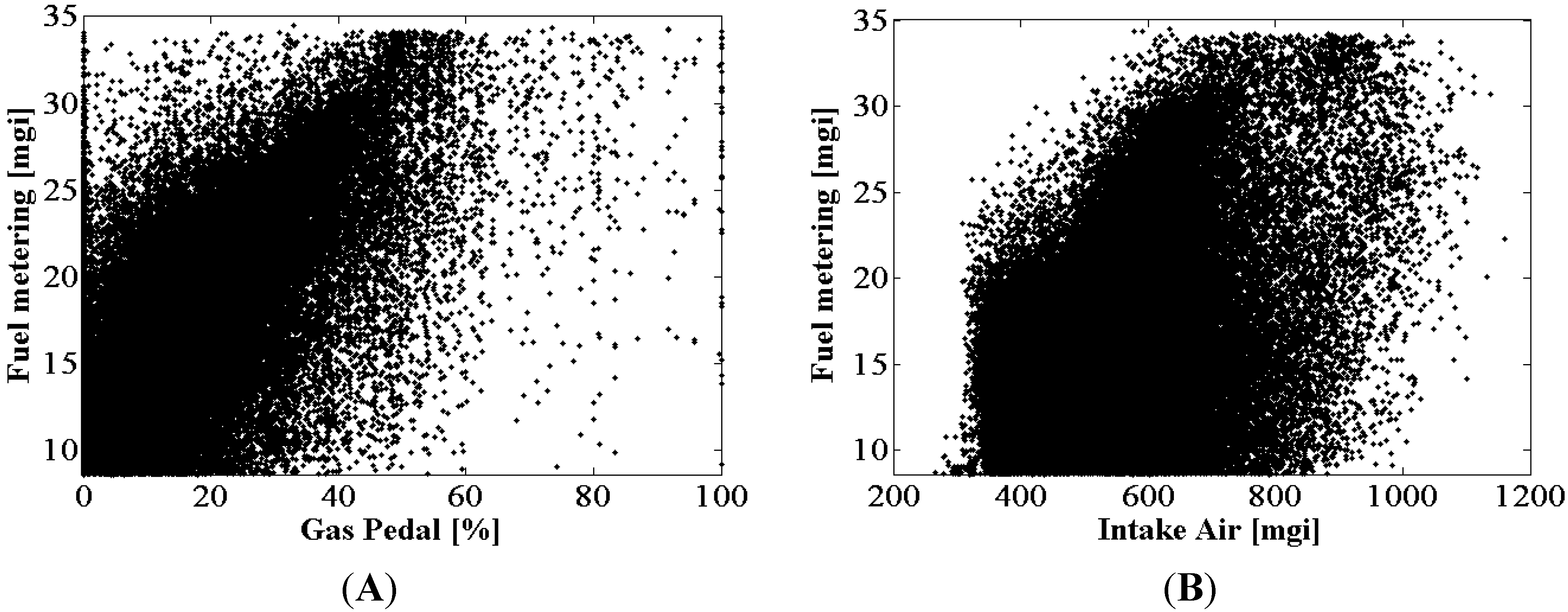
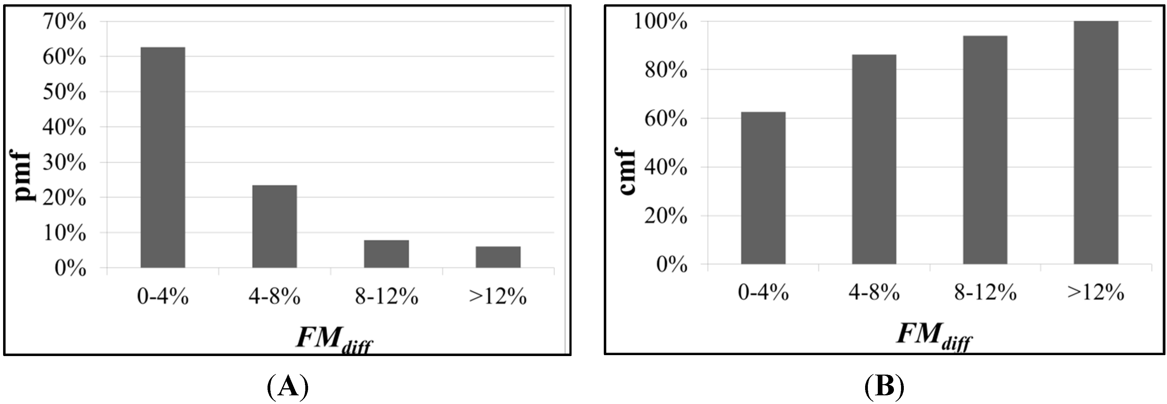
4.1. Validation of Consumption Data

Validation of consumption data is a fundamental pre-requisite of our research, as it represents the reference quantity of our research. The OBD port is the unique communication port that we have adopted for communication to the vehicle. This is not only a deliberate choice, as we are interested in adopting a variable that can be collected with ease, but it is also an explicit constraint, as we were not able to access to the CAN (connected area network) of the instrumented vehicle. In this context, the validation of the reliability of collected FCinst has been carried out indirectly. Indeed a direct correlations exists between fuel consumption and emissions. Thus, measuring emissions allows for an indirect estimation of fuel consumption. For this purpose we used the following formulation:
F C [ l s ] =   0.116 0.8242 ×   0.273 × C O 2 +   0.429 × C O 100
where CO2 and CO are respectively the instantaneous mass of CO2 and CO expressed in g/s. The development of this formulation is an outcome of experiments carried out for the DRIVE IN2 project by the Istituto Motori of the National Research Council (CNR) of Italy; more details on the aim and the results of these experiments will be given in further publications.
Comparison statistics have been reported in Figure 1, and have been based on the FMdiff parameter, defined as:
F M d i f f = |   FM ( O B D ) FM ( P E M S ) FM ( P E M S ) |
where FM ( OBD ) and FM ( PEMS ) are the values of fuel consumption read by the OBD port and estimated indirectly by using emissions. In more than 60% of the cases, differences are lower that 4%, and in general are lower than 12%. Of course neither OBD data, nor consumptions estimated from emissions could be considered un-biased. However, the concordance between the two independent instruments gives reasonable confidence on the reliability of measured fuel consumptions.
Figure 1. (A) Probability mass function (pmf) and (B) cumulative mass function (cmf) versus the difference in the consumption values measured with the two instruments (FMdiff) in the validation experiment.
Sustainability 07 14326 g001

4.2. Model Specification and Estimation of the Parameters

The actual identification of the fuel-consumptions model was based only on the data from the principal experiment. The model variables were identified by using the stepwise algorithm implemented in the Matlab Statistical Toolbox. This method easily applies to linear models and can be very effective to be adopted for real-time identification procedures.
An obvious correlation of fuel metering with the Gas Pedal and the Intake Air is confirmed by means of Figure 2.
Figure 2. Dependence of fuel metering on: (A) Gas Pedal; (B) Intake Air.
Sustainability 07 14326 g002
In addition, considering the law of traction, it is reasonable to presume a dependency of motion from the square of speed (v2) and acceleration (a). Indeed these variables were selected as more significant by the stepwise algorithm. Then the linear regression model is calibrated as follows:
FMmgi = β0 + β1 v2 + β2 a+ β3 GasPedal + β4 IntakeAir
For the specification of the model, 50 drivers were randomly taken from the sample, and the remaining subjects were used to verify the model; Fiat drivers were considered only in the validation stage. Parameters were estimated using the Matlab Statistical Toolbox, and the calibration results have been reported in Table 1, which is also where the R-square value and t-stats associated with each parameter have been reported.
Table 1 also reports the tolerance index and the VIF index (variance inflation factor), which are usually used to investigate the redundancy among the independent variables in a multiple regression model (multicollinearity test). In fact, for an explanatory i, the tolerance, Ti, is the complementary to 1 of R i 2 , where R i 2 is the coefficient of determination of a regression of explanatory on all the other explanators. Whereas the VIF index is the reciprocal of the tolerance index. In other words:
T i = 1   R i 2
V I F i =   1 T i
Table 1. Index of determination, model coefficients, and their statistical significance within the full model (identification against 50 drivers).
Constantv2aGas PedalIntake Air
β7.7500.0056.4200.2120.004
t123,00077.60084.500186,00036.400
sig.<0.001<0.001<0.001<0.001<0.001
std. β-0.2050.2250.4900.098
T-0.7970.7860.7970.763
VIF-1.2551.2731.2541.311
R20.483
std. error3.759
A tolerance less than 0.5 or a VIF higher than 2 indicates a multicollinearity problem. Because such conditions are never verified (Table 1), there is no multicollinearity among the independent variables. In the same table, the standardize coefficients (std. β) are reported; these coefficients permit the evaluation of which independent variable is more important in the explanation of the dependent variable. It is evident that, among the identified key parameters, Gas Pedal is the more important variable, while Intake Air is the least important one.
Some statistical considerations have also been carried out with reference to the performance of the model; in particular, in Figure 3, the probability mass function (pmf) and the cumulative mass function (cmf) of the absolute percentage error, ERRinst, have been depicted:
E R R i n s t ( t ) = |   x ^ i x i x i |
ERRinst represents the percentage deviation between the predicted value by the model, x ^ i , and that observed, x i , at the instant i of FMmgi.
Figure 3. (A) Probability mass function (pmf) and (B) cumulative mass function (cmf) versus the percentage error (ERRinst) of the three sub-samples.
Sustainability 07 14326 g003
Also the following statistical indicators have been reported in Table 2:
  • RMSE (root mean square error), which is the ratio between the inner deviance and the total numerosity, n
    R M S E = i = 1 n ( x i x ^ i ) 2 n
  • MAPE (mean absolute percentage error), which is a measure of accuracy of a method for constructing fitted time series values
    M A P E = 1 n   i = 1 n | x i x ^ i | x i
Table 2. RMSE and MAPE computed for the three samples.
RMSEMAPE
Specification Sample3.7900.188
Control Sample3.6700.184
Fiat Sample3.3300.161
As stated before, the aim of this work is to develop a model that can be used in an integrated simulation environment. The need for adopting independent variables that are very easily estimated by simulation platforms or collected from on-board low-cost devices has been clearly stated in Section 2. Typically, Intake Air is difficult to estimate in standard models of vehicle dynamics with enough accuracy. Thus we proceeded to the specification of another model, reduced.1. The reduced.1 model carries the same variables mentioned before except for Intake Air, namely:
FMmgi = β0 + β1 v2 + β2 a+ β3 GasPedal
The same calibration procedure was repeated and also for this case calibration results, the R-square value and t-stats associated to each parameter have been reported in Table 3.
Table 3. Index of determination and beta coefficients and their significance within the reduced.1 model (identification against 50 drivers).
Constantv2aGas Pedal
β9.5300.0057.3000.222
t238.00088.200101.000199.000
sig.<0.001<0.001<0.001<0.001
std. β-0.2280.2550.513
T-0.8450.8730.846
VIF-1.1831.1451.182
R20.476
std. error3.785
It is worth noting that, in accordance with the previous consideration about the standardized coefficients in Table 1, excluding Intake Air represents an acceptable approximation. Indeed further analyses were performed by comparison of the data obtained from the two models specified in order to demonstrate that the use of the simplified model is fully justified.
The gap between the responses of the two models has been evaluated as:
Δ ( t ) = |   FM mgi ( 1 ) FM mgi ( 2 ) FM mgi ( 1 ) |
where FM mgi ( 1 ) and FM mgi ( 2 ) are the values of fuel consumption computed in the same time instant by using the reduced and the full model, respectively.
Figure 4 shows the probability mass function (pmf) and cumulative mass function (cmf) of the values assumed by Δ in the three reference samples. Differences in the outputs of the two models are lower than 5% in more than 90% of the cases.
Figure 4. (A) The probability mass function (pmf) and (B) cumulative mass function (cmf) of the gap between the responses of the full model and the reduced.1 evaluated for the three sub-samples.
Sustainability 07 14326 g004
In order to give a final understanding of the importance of each independent variable, two further specifications of the model have been analyzed. The two models have been specified by progressively removing the v2 (model reduced.2) and the a (model reduced.3). Results associated with these models have been reported in Table 4. Removing Intake Air causes a negligible reduction of the R-square value (and consistently causes a negligible increase in the standard error of the model). The decrease of the model performance becomes significant once the reduced.2 and reduced.3 specifications are considered.
The reduced.1 model is considered to be the best trade-off between the accuracy and the practical usability we look for; for this reason further analyses described in the paper have been carried out by using the reduced.1 model.
Table 4. Index of determination and beta coefficients and their significance within the reduced.2 and reduced.3 models (identification against 50 drivers).
reduced.2 Constantv2aGas Pedal
β12.497-5.4300.255
t551.674-75.144233.576
sig.<0.001-<0.001<0.001
std. β--0.1900.590
R20.432
std. error3.940
reduced.3
β12.935--0.272
t573.849--248.090
sig.<0.001--<0.001
std. β---0.631
R20.398
std. error4.058

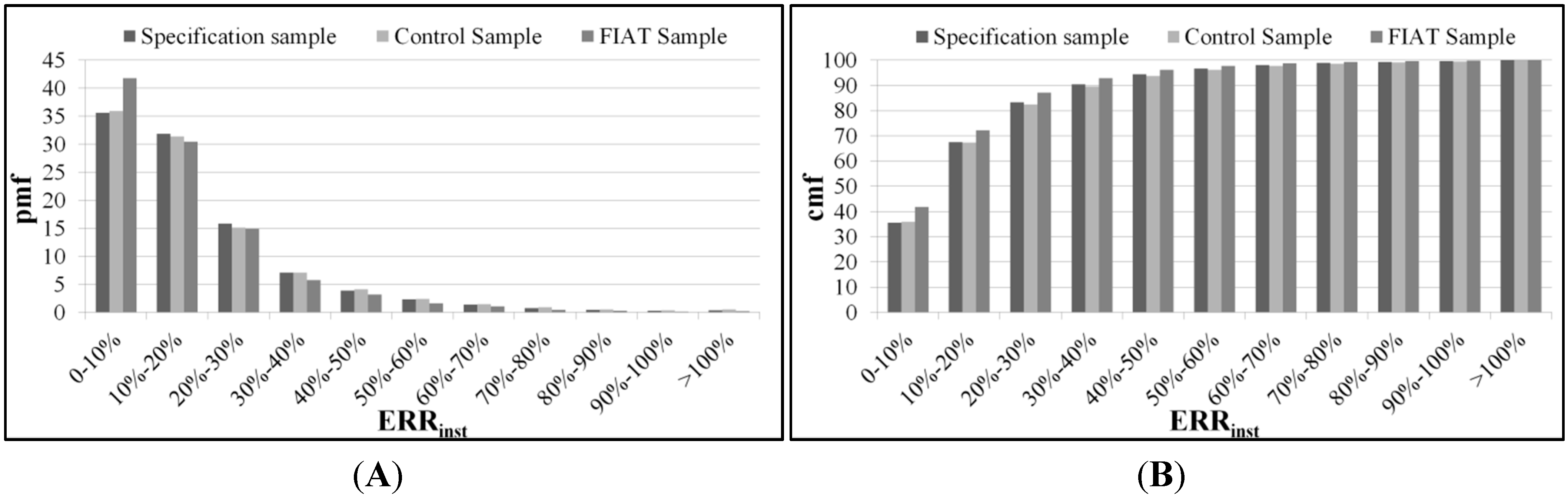
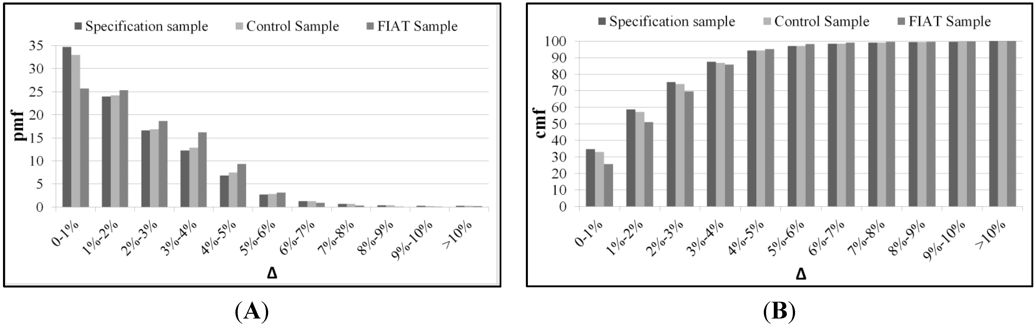
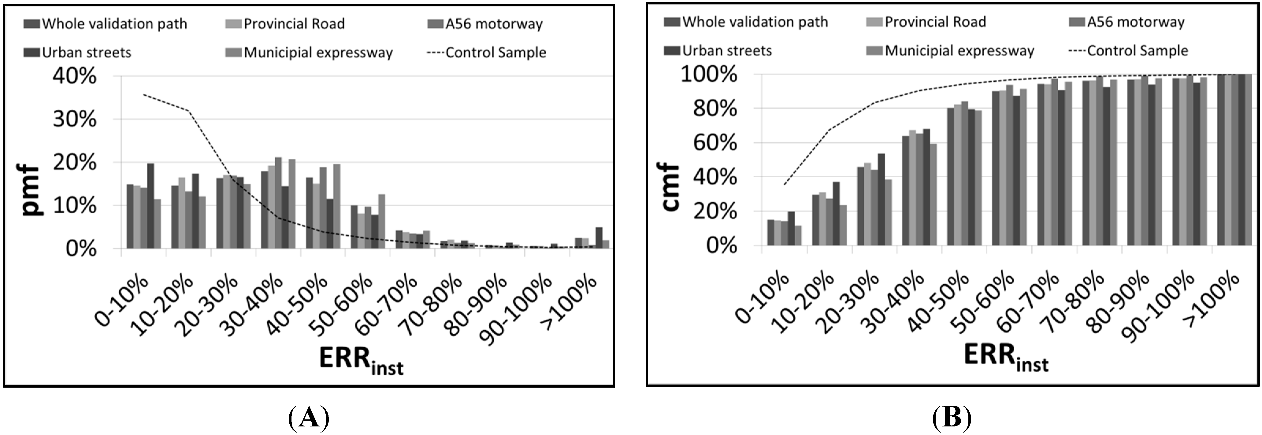
4.3. Model Transferability

In order to evaluate transferability properties of the developed model, it has been applied to the estimation of the fuel consumptions observed in the transferability experiment (see Section 3.2). Model performances are expressed again in terms of ERRinst and have been reported in Figure 5. ERRinst distribution has been computed for each of the different driving contexts studied, and for the whole validation path. The ERRinst distribution concerning the control sample of the DRIVE IN2 experiment has been also reported (dashed line) for comparison.
Figure 5. (A) Probability mass function (pmf) and (B) cumulative mass function (cmf) of the gap between the responses of the reduced.1 model once applied in the driving contexts of the validation experiment.
Sustainability 07 14326 g005
Figure 5 allows for some interesting considerations. First of all the performances of the model are fully comparable in the different contexts, although some of them are very different from each other (for example, motorway versus urban streets). Likely, this happens because the chosen independent variables are able to embed in aggregate ways the effect of different driving contexts. On the other hand, the performance of the model in these new contexts is worse. As evident from Figure 5, the incidence of small errors decreases and the incidence of medium errors increases. However, this is, in our opinion, due to the differences in the two experimental samples (e.g., 13 driving sessions vs. 100 ones—50 each in the calibration and validation dataset), rather than to the inherent characteristics of the model. This opinion will be detailed in Section 5. Of course a new transferability sample could be adopted but this goes beyond the resources now available for our work. This issue will be addressed in future research.

4.4. Parameters Dispersion

The parameters in Table 4 treat as equivalent the driving sessions of 50 randomly selected drivers. In this section, this hypothesis is removed, and the parameters of the reduced model are identified against each driving session. In Table 5 some statistics concerning the dispersion of the parameters R-square and RMSE are listed; in particular the dispersion is described by reporting the minimum, maximum, first, second and third quartile of the empirical distributions of each variable.
Although we presume that driver behavior and habits are significant factors affecting fuel consumption rates, the previous analysis does not have any behavioral implication. It is only aimed at understanding the range of variability of each of the parameters, and of the performances of the models. Interestingly when the model is specified for each driver, the R-square is (on average) higher; at the same time the RMSE is (on average) lower. Values of the coefficients are consistent with those of Table 3, except for the acceleration whose coefficients seem to have a great variability.
Table 5. The minimum, maximum, first, second and third quartiles of the values assumed by the parameters (together with R-square and RMSE) estimated for each of the trajectories in the dataset.
MinMaxQ1Q2Q3
β04.58013.5007.4408.97010.200
β11.53 × 10−41.02 × 10−24.01 × 10−36.40 × 10−37.65 × 10⁻³
β2−5.62021.2001.75011.80014.200
β30.1150.5180.1840.2360.288
R20.2260.7850.4740.5450.630
RMSE2.3205.4003.0203.4203.760

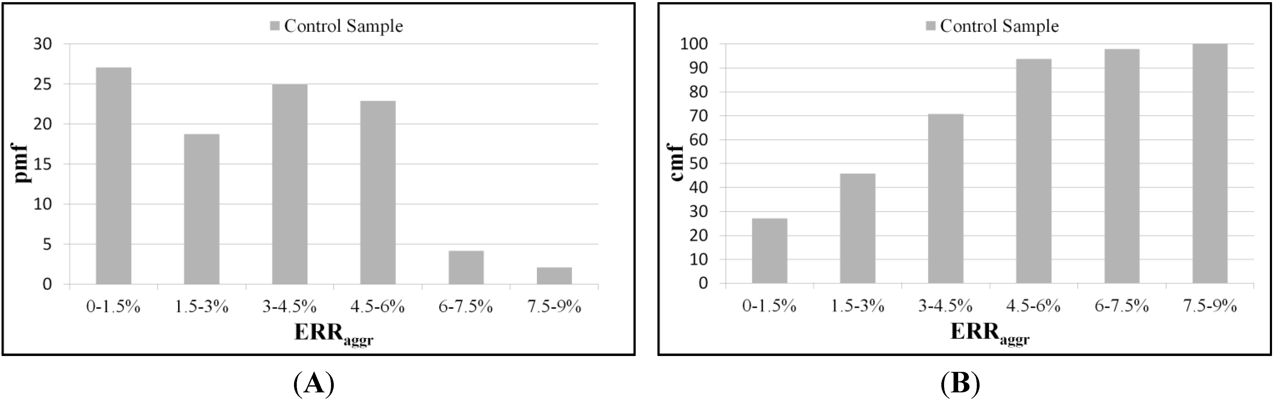
4.5. Aggregate Analysis

Another interesting point of comparison of model performances concerns the performance in terms of aggregate fuel consumption C ( T ) . Aggregated data is intended here as the temporal integration of FC inst in the total length of the driving session T, namely:
C ( T ) [ l ] = 0 T F C i n s t ( t ) · d t
Even in this case a discrepancy parameter is defined:
E R R a g g r ( t ) = |   C ^ ( T ) C ( T ) C ( T ) |
where Ĉ(T) and C(T) are the aggregate fuel consumption using the values predicted by the model and the observed ones, respectively. Figure 6 shows the probability mass function (pmf) and cumulative mass function (cmf) of the values assumed by ERRaggr variable.
Figure 6. (A) Probability mass function (pmf) and (B) cumulative mass function (cmf) versus the aggregate error evaluated in the sample used for the model verification.
Sustainability 07 14326 g006

5. Discussion

The evaluation of fuel consumption is a hot topic for the development and evaluation of Driving Assistance Systems, and the definition of a proper evaluation measure is of fundamental importance. Our results show that modelling instantaneous fuel consumption is quite difficult. Indeed in Figure 2 we showed that in about 35% of the cases, instantaneous fuel metering can be predicted with a discrepancy lower than 10% (in terms of ERRinst), but on the other hand we showed that in about 10% of the cases this discrepancy is greater than 50%. The performance of the model in terms of instantaneous fuel consumption gets worse when applied to the estimation of the fuel consumed during the transferability experiment. On the other hand two of the models presented in Section 2, those compatible with our experiments, have been calibrated using our data, and both of them present even worse performances. Indeed, the best of the functional forms within those introduced by Lee et al. [27], corresponds to our reduced.3 specification, which we showed to be less convincing than reduced.1 (Table 4); it is worth noting that in the original work the throttle was used instead of the gas pedal as independent variable, but this difference seems to be not enough to justify the great decrease in the performance of the model (the authors reported an R-square coefficient of 0.81 in their dataset). Similarly the best of the models presented in [25], the Model M, exhibits an R-square of 0.27 (and an RMSE of 4.459) once calibrated by using data of our specification sample; moreover six of the estimated coefficients (of a total of fifteen) are not statistically significant.
Another relevant point concerns the great fluctuations of the parameters (in particular for β2) estimated for each of the driving sessions (Table 5).
We argue that this great instability in the instantaneous estimation is not a matter of our experimental conditions, but rather a confirmation of the presence of several secondary components which strongly affect model estimations. One of these could be the different behaviors observable in different types of drivers. This is a point potentially relevant for our results considering the poor heterogeneity (in terms of gender and age) of the sample in the transferability experiment. Our conjecture is partially supported by the fact that results improve strongly once the same model is used to compute the total fuel consumption associated to a driving session C ^ ( T ) , in which fluctuations are averaged.
Indeed, Figure 6 has showed that in aggregated terms differences are lower than 6% in more than 90% of the cases. This is a result that could be defined as excellent according to similar estimations made in the literature [33].
However, the ERR aggr is computed on the whole trajectory duration T, while the ERR inst is computed in each instant. Thus, an interesting question to be addressed concerns the evaluation of a trade-off time interval able to compute an acceptable estimation of fuel consumption; this would be fundamental in the development of real-time eco-driving strategies.
Importantly, our results are basically based on fuel metering as observed and recorded at the OBD port, which has been showed to be quite reliable. A great advantage of the developed fuel consumption model is that, unlike most microscopic models present in literature, it can be easily integrated into much of the existing testing platforms for ADAS. This is possible because only simple data are considered in the specification of the model. Our effort toward simplification of approaches is well justified by the need for adopting online estimation and control logics in the development of ADAS. Indeed, more critical aspects in ADAS, those related to human behavior, have been proved to be effectively approachable with simple and linear models, as shown in [34,35].

6. Conclusions

Fuel consumption and CO2 emission savings can be created by adopting environmentally friendly policies, by implementing traffic congestion reducing strategies, by choosing ecological routes, and, in particular, by enacting more efficient driving styles. Our research addresses this last point through the development of real-time microscopic fuel consumption model. The data used in the paper were collected during a huge experimental campaign (more than 8000 Km of driving data over 100 subjects) near Naples, Italy, by an instrumented vehicle under extra-urban driving conditions. We proposed a simple and efficient fuel consumption model based only on data from OBD port and IMU and, therefore, one that is easy to implement in an integrated simulation environment.
The prevision accuracy of our model was verified performing both instantaneous and aggregate validations. The findings show that, despite the relative simplicity of the model’s structure and the few input variables, the proposed model provides a good estimation of the instantaneous fuel consumption and that a better estimation is obtained when the values of fuel consumption are aggregated in quite high time windows.
The peculiar aspect of proposed model, the aspect that differentiates it from the most part of microscopic models present in literature, is that it was developed specifically to be integrated into the existing ADAS testing platforms. These results justify further research efforts to extend the model’s application range to other vehicle categories and traffic contexts. Furthermore, we lay a solid foundation for an accurate and useful tool for ADAS evaluation and development and, more generally, for the estimation of the fuel consumption in simulated environments (driving simulations, model in the loop, etc.).

Acknowledgments

Data used in this work were supplied by the PON (Programma Operativo Nazionale) 2007–2013–Research Project B61H110004000005 (DRIVE IN2). Analyses and developments ware partially supported within the PON Research Project B68F12001150005 (Apps4Safety)

Author Contributions

Gennaro Nicola Bifulco initiated the project and conceptualized the paper. Maria Russo Spena analyzed the data and made contributions in writing material. Francesco Galante and Luigi Pariota made contributions in data collection, analysis and in writing the paper.

Conflicts of Interest

The authors declare no conflict of interest.

References

  1. Molenaar, R.; van Bilsen, A.; van der Made, R.; de Vries, R. Full spectrum camera simulation for reliable virtual development and validation of ADAS and automated driving applications. In Intelligent Vehicles Symposium (IV), 2015 IEEE, Proceedings of 2015 IEEE Intelligent Vehicles Symposium (IV2015), Seoul, Korea, 28 June–1 July 2015; IEEE: Piscataway, NJ, USA, 2015. [Google Scholar]
  2. Bifulco, G.N.; Pariota, L.; Galante, F.; Fiorentino, A. Coupling Instrumented Vehicles and Driving Simulators: Opportunities from the DRIVE IN2 Project. In Proceedings of 15th IEEE International Conference on Intelligent Transportation Systems, Anchorage, AK, USA, 16–19 September 2012; IEEE: Piscataway, NJ, USA, 2012. [Google Scholar]
  3. Davitashvili, T. Mathematical Modeling Pollution from Heavy Traffic in Tbilisi Streets. Available online: http://www.wseas.us/e-library/transactions/environment/2009/29-536.pdf (accessed on 16 October 2015).
  4. Pamanikabud, P. Impact Assessment of Motorway Traffic Noise Using Visualized Noise Mapping Technique. WSEAS Trans. Environ. Dev. 2009, 5, 24–33. [Google Scholar]
  5. Cartenì, A. Urban Sustainable Mobility. Part 1: Rationality in Transport Planning. Available online: http://www.transportproblems.polsl.pl/pl/Archiwum/2014/zeszyt4/2014t9z4_04.pdf (accessed on 19 October 2015).
  6. Chi, Y.; Guo, Z.; Zheng, Y.; Zhang, X. Scenarios Analysis of the Energies’ Consumption and Carbon Emissions in China Based on a Dynamic CGE Model. Sustainability 2014, 6, 487–512. [Google Scholar] [CrossRef]
  7. Zhang, X.; Xie, J.; Rao, R.; Liang, Y. Policy Incentives for the Adoption of Electric Vehicles across Countries. Sustainability 2014, 6, 8056–8078. [Google Scholar] [CrossRef]
  8. Sivak, M.; Schoettle, B. Eco-driving: Strategic, tactical, and operational decisions of the driver that influence vehicle fuel economy. Transp. Policy 2012, 22, 96–99. [Google Scholar] [CrossRef]
  9. D’Acierno, L.; Montella, B.; Gallo, M. A fixed-point model and solution algorithms for simulating urban freight distribution in a multimodal context. J. Appl. Sci. 2011, 11, 647–654. [Google Scholar]
  10. Gori, S.; La Spada, S.; Mannini, L.; Nigro, M. Emission dynamic meso-simulation model to evaluate traffic strategies in congested urban networks. IET Intell. Transp. Syst. 2014, 9, 333–342. [Google Scholar] [CrossRef]
  11. Mauro, R.; Giuffrè, O.; Grana, A.; Chiappone, S. A statistical Approach for Calibrating a Microsimulation Model for Freeways. WSEAS Trans. Environ. Dev. 2014, 10, 496–508. [Google Scholar]
  12. Donateo, T. CO2 impact of intelligent plugin vehicles. WSEAS Trans. Environ. Dev. 2013, 9, 240–252. [Google Scholar]
  13. De Luca, S.; di Pace, R.; Marano, M. Modelling the adoption intention and installation choice of an automotive after-market mild-solar-hybridization kit. Transp. Res. Part C 2015, 56, 426–445. [Google Scholar] [CrossRef]
  14. Ntziachristos, L.; Gkatzoflias, D.; Kouridis, C.; Samaras, Z. COPERT: A European road transport emission inventory model. In Information Technologies in Environmental Engineering; Springer: Berlin, Germany, 2009; pp. 491–504. [Google Scholar]
  15. Brzezinski, D.J.; Newell, T.P. MOBILE 6 A Revised Model for Estimation of Highway Vehicle Emissions. Emiss. Inventory Living Glob. Environ. 1998, 1, 526–567. [Google Scholar]
  16. Koupal, J.; Cumberworth, M.; Michaels, H.; Beardsley, M.; Brzezinski, D.J. Design and Implementation of MOVES: EPA’s New Generation Mobile Source Emission Model. Available online: http://www3.epa.gov/ttn/chief/conference/ei12/mobile/koupal.pdf (accessed on 16 October 2015).
  17. Hui, G.; Zhang, Q.Y.; Yao, S.; Wang, D.H. Evaluation of the International Vehicle Emission (IVE) model with on-road remote sensing measurements. J. Environ. Sci. 2007, 19, 818–826. [Google Scholar]
  18. Zhou, X.; Huang, J.; Weifeng, L.; Li, D. Fuel consumption estimates based on driving pattern recognition. In Green Computing and Communications (GreenCom), 2013 IEEE and Internet of Things (iThings/CPSCom), IEEE International Conference on and IEEE Cyber, Physical and Social Computing, Proceedings of 2013 IEEE International Conference on Green Computing and Communications (GreenCom) and IEEE Internet of Things(iThings) and IEEE Cyber, Physical and Social Computing(CPSCom), Beijing, China, 20–23 August 2013; IEEE: Piscataway, NJ, USA, 2013. [Google Scholar]
  19. Post, K.; Kent, J. H.; Tomlin, J.; Carruthers, N. Fuel consumption and emission modelling by power demand and a comparison with other models. Transp. Res. Part A General 1984, 18, 191–213. [Google Scholar] [CrossRef]
  20. Akcelik, R. Efficiency and drag in the power-based model of fuel consumption. Transport. Res. B Methodological 1989, 23, 376–385. [Google Scholar] [CrossRef]
  21. Leung, D.Y.C.; Williams, D.J. Modeling of motor vehicle fuel consumption and emissions using a power-based model. Environ. Monit. Assess. 2000, 65, 21–29. [Google Scholar] [CrossRef]
  22. Rakha, H.A.; Ahn, K.; Trani, A. Development of VT-Micro model for estimating hot-stabilized light duty vehicle and truck emissions. Transp. Res. Part D Transp. Environ. 2004, 9, 49–74. [Google Scholar]
  23. Wong, J.Y. Theory of Ground Vehicles; John Wiley & Sons: Hoboken, NJ, USA, 2001. [Google Scholar]
  24. Rakha, H.A.; Ahn, K.; Moran, K.; Searens, B.; Van den Bulck, E. Virginia Tech Comprehensive Power-Based Fuel Consumption Model: Model development and testing. Transp. Res. Part D Transp. Environ. 2011, 16, 492–503. [Google Scholar] [CrossRef]
  25. Ahn, K. Microscopic Fuel Consumption and Emission Modeling. Master’s Thesis, Virginia Polytechnic Institute and State University, Blacksburg, VA, USA, 1998. [Google Scholar]
  26. Barth, M.; An, F.; Younglove, T.; Scora, G.; Levine, C.; Ross, M.; Wenzel, T. Development of a Comprehensive Modal Emissions Model. Available online: http://onlinepubs.trb.org/Onlinepubs/nchrp/nchrp_w122.PDF (accessed on 16 October 2015).
  27. Lee, M.G.; Park, Y.K.; Jung, K.K.; Yoo, J.J. Estimation of Fuel Consumption using In-Vehicle Parameters. Int. J. u- e-Serv. Sci. Technol. 2011, 4, 37–46. [Google Scholar]
  28. Van der Voort, M.; Dougherty, M.S.; van Maarseveen, M. A prototype fuel-efficiency support tool. Transp. Res. Part C 2001, 9, 279–296. [Google Scholar] [CrossRef]
  29. Larsson, H.; Ericsson, E. The effects of an acceleration advisory tool in vehicles for reduced fuel consumption and emissions. Transp. Res. Part D 2009, 14, 141–146. [Google Scholar] [CrossRef]
  30. Montella, A.; Pariota, L.; Galante, F.; Imbriani, L.L.; Mauriello, F. Prediction of drivers’ speed behavior on rural motorways based on an instrumented vehicle study. Transp. Res. Rec. 2014, 2434, 52–62. [Google Scholar] [CrossRef]
  31. Bifulco, G.N.; Galante, F.; Pariota, L.; Russo Spena, M. Identification of driving behaviors with computer-aided tools. In Computer Modeling and Simulation (EMS), UKSim-AMSS 6th European Modelling Symposium, Proceedings of the 2012 Sixth UKSim/AMSS European Symposium on Computer Modeling and Simulation, Valetta, Malta, 14–16 November 2012; IEEE: Piscataway, NJ, USA, 2012. [Google Scholar]
  32. Bifulco, G.N.; Pariota, L.; Simonelli, F.; di Pace, R. Real-time smoothing of car-following data through sensor-fusion techniques. Procedia Soc. Behav. Sci. 2011, 20, 524–535. [Google Scholar] [CrossRef]
  33. Alessandrini, A.; Filippi, F.; Ortenzi, F. Consumption Calculation of Vehicles Using OBD Data. Available online: http://www3.epa.gov/ttnchie1/conference/ei20/session8/aalessandrini.pdf (accessed on 19 October 2015).
  34. Pariota, L.; Bifulco, G.N. Experimental evidence supporting simpler Action point paradigms for car-following. Transp. Res. Part F 2015. [Google Scholar] [CrossRef]
  35. Pariota, L.; Bifulco, G.N.; Brackstone, M. A linear dynamic model for driving behaviour in car-following. Transp. Sci. 2015. [Google Scholar] [CrossRef]

