Article

Coupling and Coordinated Development of Urbanization and Ecological Environment in China and Its Spatio-Temporal Characteristics

School of Economics and Management, Lanzhou Institute of Technology, Lanzhou 730050, China
*
Author to whom correspondence should be addressed.
Sustainability 2026, 18(9), 4559; https://doi.org/10.3390/su18094559
Submission received: 22 March 2026 / Revised: 30 April 2026 / Accepted: 2 May 2026 / Published: 5 May 2026
(This article belongs to the Section Social Ecology and Sustainability)

Abstract

The stability and health of the ecological environment are the premise of urbanization development, and promoting their coordinated advancement constitutes the goal of sustainable social development. This research employs panel data from 30 Chinese provinces and provincial-level municipalities over the period 2011–2023 to construct a comprehensive evaluation index system for urbanization and ecological environment (U-EE). The coupling coordination degree (CCD) model is used to evaluate the coordinated development level of U-EE. Combining the Dagum–Gini index and decomposition (DGID), the spatial autocorrelation model (SAM) and trend surface analysis (TSA), the evolution characteristics and changing trends of the U-EE coordination degree (D-UEE) in both time and space are explored. It is found that, first of all, the CCD model results show that D-UEE is not high overall, yet exhibits a consistent year-on-year upward trend. Secondly, the DGID results show that the intra-group differences among the four regions—namely, the eastern, central, western and northeastern regions—are decreasing year by year, among which the eastern region has the largest difference and the northeastern region has the smallest difference. In terms of inter-group differences, the east–west disparity is the largest, whereas the central–northeast difference is the smallest. Thirdly, the global Moran’s index (GMI) results show that D-UEE presents significant spatial aggregation distribution characteristics and there is a positive correlation phenomenon. Fourthly, from the perspective of the local Moran’s index (LMI), most of the regions are concentrated in the first and third quadrants, corresponding to HH and LL types, exhibiting significant positive spatial autocorrelation and clustering patterns characterized by spatial homogeneity. Fifthly, the results of TSA show that the spatial distribution of D-UEE is high in the eastern and low in the western regions, and high in the southern and low in the northern regions. Through analysis of the results, it is evident that the intra-regional gap in the country is narrowing, but the east–west gap is still the most important reason for spatial differentiation. There are still some incoordination issues between the U-EE systems, but they are continuously improving and moving in a positive direction.

1. Introduction

Against the backdrop of sustained regional economic development, urbanization has become the primary indicator of regional economic growth, as cities possess superior educational resources and advanced medical facilities. This causes population migration and mobility to become active, leading to continuous growth in urban populations. By the end of 2024, China’s urban resident population stood at 943.50 million, an increase of 10.83 million compared to the end of 2023. The rural resident population was 464.78 million, a decrease of 12.22 million. The urbanization rate of the permanent population was 67.00%, an increase of 0.84 percentage points compared to the end of 2023 [1]. The urbanization rate of the population continues to rise. However, it is worth noting that the rapid development of urbanization will bring certain negative impacts on the ecological environment and people’s lives. The growth of urban populations has rendered the previously stable size of cities inadequate to meet the demands of a continuously expanding population, resulting in increasingly congested city roads. Urban development requires more resources, more housing, and so on. Therefore, during the process of urbanization, substantial tracts of land are allocated to expand the scale of urban construction, such as the construction of houses, factories, roads, and so on. The city is the main place for people’s survival and recreation. However, the rapid acceleration of urbanization has resulted in the excessive exploitation of land resources, resulting in a steady decline in cultivated land, forested areas, and other natural ecosystems. This then leads to serious soil erosion, land desertification, air pollution, and other problems. The ecological problems brought by urbanization development have attracted people’s attention. The primary objective of our research is to balance the coordinated and sustainable development of urbanization and the ecological environment (U-EE).
There has been a lot of research on the topic of urbanization and ecology. Mcintyre et al. provide a cross-disciplinary, quantitative description of urban ecosystems that accounts for their dynamic and heterogeneous physical and social characteristics [2]. Following cross-disciplinary quantitative research, Young established urban ecology as an integrative field bridging the social and ecological sciences. Studies also claim that urban ecology as a field has a wider depth, informing and aiding urban ecology and planning research [3]. Urban ecology assesses the benefits of urban green spaces, vegetation areas, and water bodies for health and well-being [4]. With the development of urban ecology, Katte et al. proposed a complementary framework of urban ecology, E-LAUD, which considers that ecosystems interact with land use, architecture, and urban design. It is recommended that the E-LAUD framework be incorporated into urban planning, forming the context for a new interdisciplinary research program on the ecological resilience of urban ecosystems, and contribute to the promotion of ecosystem services [5]. For the classical concept of urbanization, little consideration is given to the fact that cities expand rapidly in spatially complex, non-linear ways. Therefore, Ramalho et al. considered this issue and, in combination with the characteristics of urbanization, outlined the framework of emerging urban ecology [6]. Urban ecology has gradually evolved into a truly cross-disciplinary enterprise. Cities are complex adaptive systems with spatial heterogeneity [7,8]. Due to the spatial complexity of urban ecosystems, there are many researchers who have begun to study them from many different perspectives. Tanner et al. believe that each perspective can offer some help to the social and ecological sciences [9]. For example, Wang et al. combined a geographical model and used a geographical detector to explore the driving factors of the coordination degree of the urbanization and ecological environment composite system (CUECS) [10]. Some researchers combined econometric models to study the interaction and influencing factors between urbanization and ecology, such as classical cointegration regression (CCR), dynamic ordinary least squares (DOLS), and fully modified ordinary least squares (FMOLS) models, which further confirmed the nature of the relationship among natural resources (NR), urbanization, economic growth (EG), and the ecological footprint (EF) [11]. Some studies use multiple linear regression models to analyze the influencing factors of urban ecological resilience, influencing factors of urban ecological resilience, including biophysical and socio-economic variables [12]. Some studies use a coupling coordination degree model to quantitatively analyze the coordinated development trend between urbanization and the ecological environment [10,13]. Some studies explore the spatial differences between cities and ecology from the perspective of space. For instance, spatial lag models (SLM) and ordinary least squares (OLS) regression models have been employed to investigate the spatiotemporal patterns and factors influencing ecological conservation in the megacity of Kolkata, India [14]. Additionally, methods such as kernel density estimation and the Dagum–Gini index were employed to investigate the temporal evolution, spatial distribution, and spatial variation characteristics of urban ecological resilience [15]. Compared with the traditional panel regression model, which only relies on statistical data for analysis, the existing research has begun to try to integrate new technologies to improve the research accuracy. Didmanidze, O. N. et al. can effectively improve the accuracy and spatial coverage of original data through remote sensing technology. On this basis, artificial intelligence and machine learning methods can be further used to simulate and predict future development scenarios, providing more scientific support for regional development trends [16].
Maintaining the coordinated development of U-EE is of paramount importance. Although the existing research has analyzed the mutual influence of U-EE from multiple perspectives. However, there are few analyses of the spatial differences in their coordination degrees. Therefore, based on the analysis of the development of U-EE coordination and the spatial model, this study further examines the spatial differentiation in the degree of coordination. Firstly, the sample data of 30 regions (excluding Xizang, Hong Kong, Macao, and Taiwan regions of China, the same below) in China from 2011 to 2023 are selected, and the comprehensive index evaluation system for U-EE is constructed using the entropy weight method (EWM). Secondly, the CCD model is used to measure the CCD of U-EE. Thirdly, the Dagum–Gini index and decomposition (DGID) are used to analyze the regional differences in the U-EE coordination degree (D-UEE). Fourthly, the spatial autocorrelation model (SAM) is used to analyze the degree of spatial correlation of D-UEE. Finally, a trend surface analysis (TSA) model is used to examine the distribution characteristics and changing trend of D-UEE in spatial geography. Through systematic research, this facilitates a more precise understanding of the spatial distribution patterns of D-UEE, and it can be intuitively seen which regions exhibit high D-UEE levels and which areas need to be improved. It has theoretical and practical significance for improving the D-UEE and promoting regional coordinated and healthy development. The research framework for this study is shown in Figure 1.

2. Materials and Methods

2.1. Data Selection

In the construction process of the comprehensive evaluation index system of urbanization, we further supplement the relevant literature basis and policy planning support to make the index selection more reasonable. Yao, J. et al. used indicators such as science, culture and medical level as the evaluation system of urbanization [17]. Yang, M. et al. used economic, ecological, infrastructure and other indicators as the evaluation system of urbanization [18]. In addition, Chen, R. et al. selected population, economic, social, ecological and other indicators as the evaluation system of urbanization [19]. According to the national new urbanization plan, the indicators of new urbanization mainly include the urbanization rate of permanent population, education, basic medical and health care, infrastructure, resources and environment and other aspects [20,21]. Referring to the existing literature and relevant policy planning, the urbanization index system of this study is constructed from the five aspects of residents’ livelihoods, economic development, education level, medical level and public infrastructure. In terms of residents’ livelihoods, the density of urban populations provides clear insights into population distribution within cities. Areas with high population density typically feature more shopping malls, cinemas, gyms, and other recreational facilities, enriching residents’ lives. Residents’ actual purchasing power forms the foundation for sustaining their standard of living. Therefore, urban residents’ livelihoods are reflected through indicators such as population density of urban areas (UAPD) [4], per capita disposable income of households by region (RPCDI) [17,18,19], and total retail sales of consumer goods (CGTRS) [22]. In terms of economic development, gross domestic product (GDP) serves as a measure of the overall scale and growth rate of an economy. The tertiary industry has a wide range of fields, including finance, scientific and technological services, which have high added value and can create greater economic value for the city. Therefore, according to the per capita regional GDP [23,24], the proportion of value added contributed by the tertiary industry (TIAV) in the regional GDP represents the economic development level of the city [25]. In terms of education, a high collection of public libraries is an important achievement and symbol of urban cultural construction, reflecting the cultural deposits and connotations of a city, and helping to enhance the cultural strength and image of a city. Colleges and universities are an important base for cultivating talents, and a higher average number of students means that a city can cultivate and attract more high-quality talents, thereby providing robust human capital and institutional support for urban development, and advancing scientific and technological innovation as well as societal progress. Therefore, using the collections of public libraries per person (PLC) [19], the higher education enrolment per 100,000 population (HEE) [19] indicates the educational level of a city. In terms of the level of medical development, hospital beds in healthcare institutions directly reflect their inpatient care capacity. More beds usually mean stronger medical service supply capacity to meet the hospitalization needs of more patients. Health technicians are the main body of providing medical services, and more health technicians mean that they can provide patients with more timely and comprehensive medical services and improve medical efficiency. Therefore, the beds in health care institutions per 1000 persons (HCIB) [22], the health technical personnel in health care institutions per 1000 persons (HCIHTP) [19] are used to indicate the medical level of a city. In terms of public infrastructure, the per capita urban road area reflects the investment and development degree of the city in transportation road construction. A higher per capita urban road area means that the city has more sufficient road resources, which can provide a more spacious and comfortable travel environment for residents and help alleviate traffic congestion. The per capita park green space area reflects urban residents’ access to park and green space resources, providing residents with space for walking, running, fitness, play, and other leisure and entertainment. It alleviates life and work-related stress while enhancing residents’ physical and mental well-being and overall quality of life. Therefore, the per capita area of paved roads (PCAPR) [17], public recreational green space per capita (PCPRGS) [25] are used to represent the public infrastructure of the city.
In this study, the ecological environment index system is constructed based on three aspects of ecological basis, ecological governance and air pollution. In terms of ecological basis, the green coverage rate of the built-up area reflects the extent to which a city’s green plants cover the ground. A higher green coverage rate of the built-up area can improve the air quality of the city and promote the coordination and balance between urban development and the environment. Per capita water resources serve as an indicator of the relative abundance or scarcity of water resources within a given region. A high per capita water resource volume indicates that water resources are relatively abundant and can better meet the living needs of residents. On the contrary, the region faces the problem of water shortage, which may restrict economic and social development. Forest coverage serves as an indicator of both the abundance of forest resources and the quality of the regional ecological environment. Therefore, the green covered rate of built districts (BDGCR) [17], per capita water resources (PCWR) [17], and the forest coverage rate (FCR) [17] are selected as the ecological basic indicators. In terms of ecological governance, the comprehensive utilization rate of general industrial solid waste serves as an indicator of the extent to which such waste is resourcefully recovered and reused. Improving the comprehensive utilization rate of industrial waste can put a large number of originally discarded resources back into the production process, promoting resource recycling, reduce ecological pressure, and enhance the quality of the ecological environment. The daily treatment capacity of urban sewage refers to the amount of sewage that the urban sewage treatment system can treat in one day. The effective treatment of urban sewage can reduce the pollution of rivers and lakes and protect water resources. Timely cleaning and transportation of household garbage can reduce the accumulation of garbage in residential areas, streets and other places, improve environmental sanitation, protect the ecological environment and residents’ health. Therefore, the integrated reuse rate of industrial solid wastes (ISWIRR) [17], daily disposal capacity of city sewage (CSDDC) [25], and the volume of domestic garbage collected and transported (DGCTV) are selected as ecological governance indicators. In terms of air pollution, air pollutants are caused by human activities or natural processes that cause certain polluting substances to enter the air. When a certain concentration is reached, it will cause ecological harm and harm people’s health. Therefore, particulate matter (PM) emission, chemical oxygen demand (COD) emission [17], and S O 2 emission [26] are selected as air pollution indicators.
The urbanization subsystem covers the core dimensions of population agglomeration, economic expansion, education, medical care and urban construction, which together reflect the comprehensive level of urbanization construction. The ecological environment subsystem focuses on the natural resource foundation, ecological restoration and ecological pollution, representing the basic resource constraints and environmental support conditions that urban sustainable development faces. These indicators can jointly scientifically reflect the mutual restraint and adaptation between the urbanization process and the evolution of the ecological environment, and further support the reasonable assessment of the degree of coupling coordination within the research framework.
Before using the entropy weight method to determine the index weight, we first conduct a variance inflation factor (VIF) test for urbanization and ecological environment indicators to avoid the possible multicollinearity among variables. The test results are shown in Table 1 and Table 2.
The VIF results in Table 1 and Table 2 show that the VIF values for all variables are less than 10, indicating that there is no obvious multicollinearity among variables [27]. This conforms to the requirement of the objective weighting method for the independence of indicators. Table 3 shows the detailed indicator system.
According to Table 3, it can be found that, in the indicator system of EE, the weight of PCWR is 0.308, which is much higher than other indicators. This requires the consideration of the question of whether the results will be dominated by PCWR.
Considering whether the weight of each variable is robust and in order to make the results more convincing, Monte Carlo sensitivity analysis (MCSA) was added to the manuscript, adding ±3% random additions to all indicators. The Monte Carlo sensitivity analysis is a method used to determine how changes in input variables affect the prediction results of the model [28]. A single variable value is adjusted by a predetermined amount and the simulations are run one by one, but these changes should not affect the forecast [29]. Recalculated entropy is weighted 50 times repeatedly. The results are shown in Table 4.
Results show that the dominant indicator remained ranked first in all simulations. The coefficient of variation (CV) of weights was below 0.1, indicating high stability [30]. Although the weight of per capita water resources is higher, per capita water resources do not directly affect the results of CCD. And that means that other indicators in the ecosystem (such as the green covered rate of built districts, forest coverage rate, integrated reuse rate of industrial solid wastes, etc.) also have an important impact on the comprehensive score, and there are also significant spatial differences. In response to the issue of the high weighting assigned to water resources, we will examine the reasons for this high weighting by considering both the characteristics of regional resources and the attributes of the indicators.
From the regional natural characteristics, the western and northern parts of the study area belong to the arid and semi-arid ecologically fragile zone. The spatial and temporal distribution of precipitation is uneven, and water resources are the core limiting factor for regional ecosystem maintenance, urbanization construction and industrial development. Compared with other ecological indicators such as land, vegetation and atmospheric environment, the water resource supply capacity has an irreplaceable constraint on the regional ecological basis. Therefore, compared with other ecological indicators, it has a higher basic contribution.
From the perspective of indicator attributes, the spatial differences in other ecological indicators, such as green coverage and air quality, are relatively gentle at the regional level. However, per capita water resources are affected by geographical location and climatic conditions, so the regional differentiation is strong, and the index dispersion and sample discrimination are significantly higher. In the weighting logic of the entropy weight method, the higher the data discrimination degree is and the greater the amount of effective evaluation information is, the higher the corresponding weight will be, which fully conforms to the objective weighting principle of the entropy weight method, which is that the greater the difference is, the higher the weight is [31].

2.2. Research Model

2.2.1. Entropy Weight Method

Considering the dimensional inconsistency among different variables, firstly, the variables are processed by using max-min standardization, and the calculation formula is as follows [32,33].
P o s i t i v e   i n d i c a t o r s   r i j = x i j m i n i { x i j } m a x i { x i j } m i n i { x i j }
N e g a t i v e   i n d i c a t o r s   r i j = m a x i { x i j } x i j m a x i { x i j } m i n i { x i j }
In Formulas (1) and (2), i denotes the indicator and j denotes the region. x i j denotes the original index value. r i j represents the normalized value. m i n i { x i j } denotes the minimum value. m a x i { x i j } denotes the maximum value.
The normalized value of r i j is given by equation y i j , in Formula (3) [34,35].
y i j = r i j i = 1 m r i j
The entropy e i and weight ω i associated with the value index are computed using the EWM [36,37,38,39].
e i = k y i j ln ( y i j ) , k = 1 ln ( n )
ω i = g j i = 1 m g j , g j = 1 e j
However, in Formulas (4) and (5), ω i and y i j are employed to compute the comprehensive evaluation index value v j for both the urbanization and ecological system, as in Formula (6) [37,40,41].
v j = i = 1 m ω j y i j

2.2.2. Coupling Coordination Degree Model

This study uses the CCD model to analyze the interplay between the urbanization system and the ecosystem. The CCD model is formulated as follows [42,43,44,45].
C = U · E ( U + E 2 ) 2
T = α U + β E
D = C × T
In (7), C represents the U-EE coordination degree, U represents the comprehensive evaluation index of the urbanization system, and E denotes the comprehensive EE index. Here, U and E are calculated using the EWM. T represents the degree of influence of the U-EE [44]. In Formula (8), α and β represent the weights of U-EE. Liu, J. et al. argue that the coordinated development of energy, economy and ecosystems is of equal importance, and set the values of the coefficients as α = β = δ = 1 / 3 [23]. Ye, S. et al., when using a CCD model to assess the degree of coupling and coordination between Resource and Environmental Carrying Capacity (RECC) and social development quality (SDQ), consider RECC and SDQ to be equally important [46]. Zhai, X. et al., when assessing the degree of coordination between high-quality development (HQD) and high-level protection (HLP), considered HQD and HLP to be of equal strategic importance, and set the values of α and β at 0.5 [47]. Based on the above research, the CCD model treats both subsystems as equally important in the social sciences, regardless of whether there are three or two subsystems. Consequently, when using the CCD to assess the degree of coupling and coordination between U and EE, we also regard these two systems as equally important, so α = β = 0.5 [43]. In Formula (9), D represents the D-UEE [45]. The current evaluation results are based on the preset assumption of equal importance of the urbanization subsystem and ecological environment subsystem ( α = β = 0.5 ), and the model results may be affected if different α and β values are assigned. The classification of CCD is presented in Table 5 [33,48,49].

2.2.3. Dagum–Gini Index and Decomposition

Compared with the conventional Gini index, the Dagum–Gini index enables a more nuanced analysis of inter-regional disparities among samples, as well as their detailed distributional characteristics [50]. The calculation formula is presented below [51,52,53,54].
G = j = 1 k h = 1 k i = 1 n j r = 1 n h | C C D j , i C C D h , r | 2 n 2 C C D ¯
In Formula (10), n denotes the number of research areas. k indicates that the region is divided into k groups. n j denotes the number of districts in group j . n h denotes the number of districts in group h . C C D j , i represents the CCD value of the i th region in group j . C C D h , r represents the CCD value of the r th region in the h group. C C D ¯ represents the average value, C C D ¯ = i = 1 n C C D i / n   [55].
Suppose P has a group of n units. Due to the differences between regions, n regions are divided into K groups, and any group n j ( j = 1 , , k ) is subgroup P j [56,57,58,59,60,61]. The internal Gini index of P j is G j j .
G j j = i = 1 n j r = 1 n j | C C D j , i C C D j , r | 2 n j 2 C C D ¯ j
The extended Gini index between the two subgroups P j and P h is G j h .
G j h = i = 1 n j r = 1 h j | C C D j , i C C D h , r | 2 n j n h ( C C D ¯ j + C C D ¯ H )
Formulas (11) and (12), G j j only involve intra-group differences in P j . G j h involves the group difference between P j and P h . A two-period Gini decomposition is carried out below [57].
G = j = 1 k ( i = 1 n j r = 1 n j | C C D j , i C C D j , r | ) 2 n 2 C C D ¯ + 2 j = 2 k h = 1 j 1 ( i = 1 n j r = 1 n h | C C D j , i C C D h , r | ) 2 n 2 C C D ¯ = G ω + G g b
In Formula (13), where G ω denotes the intra-group Gini index. G g b denotes the inter-group Gini index.
The weighted average of G ω and G g b is denoted as P j , as given by Formula (14).
P j = n j n , s j = n j C C D j n C C D
Then, the Gini index is Formula (15).
G = j = 1 k G j j P j s j + 2 j = 2 k h = 1 j 1 G j h ( P j s h + P h s j ) = G ω + G g b
d j h = 0 d F j ( y ) 0 y ( y x ) d F h ( x )
In Formula (16), d j h is defined as the weighted average of y j i y h r . y j i belongs to P j , and y h r belongs to P h . y ¯ j > y ¯ h [56]. In this study, y is the D-UEE.
The first-order moment of transvariation is shown as in Formula (17) [56].
p j h = 0 d F h ( y ) 0 y ( y x ) d F j ( x )
In Formula (17), p j h is defined as the weighted average of y h r y j i . y h r > y j i and y ¯ h > y ¯ j .
D j h = d j h p j h d j h + p j h
D j h is the maximum likelihood ratio [52].
G n b = j = 2 k h = 1 j 1 G j h ( p j s h + p h s j ) D j h
Formula (19), G n b quantifies the contribution of intra-group Gini inequality to the overall Gini ratio G [56].
G t = j = 2 k h = 1 j 1 G j h ( p j s h + p h s j ) ( 1 D j h )
In Formula (20), G t measures the net contribution of the extended Gini inequality between to the total Gini ratio G [56].
Therefore, the inter-group Gini index G g b can be expressed as Formula (21).
G g b = j = 2 k h = 1 j 1 G j h ( P j s h + P h s j ) = j = 2 k h = 1 j 1 G j h ( p j s h + p h s j ) D j h + j = 2 k h = 1 j 1 G j h ( p j s h + p h s j ) ( 1 D j h ) = G n b + G t
The Gini index may be divided into three components, including G ω , G n b , G t .
The relationship between the three is G = G ω + G n b + G t [52,53,56,57].

2.2.4. Spatial Autocorrelation Model

In the spatial autocorrelation analysis (SAM) and spatial econometric analysis, this study refers to the research of Griffith, D. A., Janatabadi, F. et al., and Yin, F. et al. The 0–1 binary spatial weight matrix constructed by a spatial adjacency relationship is defined as an adjacency relationship if there is a common boundary between two spatial units, and the weight is assigned 1, otherwise 0 [58,59,60]. Global indicators of spatial association (GISA) can measure the degree of spatial correlation of D-UEE. The global Moran’s index (GMI) is used here [62,63,64,65].
I = i = 1 n j i n ω i j ( ( x i x ¯ ) ( x j x ¯ ) ) S 2 i = 1 n j 1 n ω i j i j
In Formula (22), ω i j denotes the spatial weighting matrix. S 2 = 1 n i = 1 n ( x i x ¯ ) 2 , x ¯ = 1 n i = 1 n x i [66,67].
The significance of the GMI was determined using the Z-score test [66,67,68].
Z = ( I ) = I E ( I ) V A R ( I )
Local indicators of spatial association (LISA) quantify spatial autocorrelation among neighboring geographic units. The local Moran’s index (LMI) is used to measure it [69,70].
I i = x i x ¯ S i 2 j = 1 , j i n ω i j ( x j x ¯ )
In Formula (24), S i 2 = j = 1 , j i n ω i j ( x j x ¯ ) 2 n 1 .

2.2.5. Trend Surface Analysis

TSA is regarded as a polynomial function of geographical coordinates, usually decomposed into trend surfaces and residual surfaces [71,72]. The model can simulate the distribution characteristics and regional change trend of the observed data in spatial geography. The second-order polynomial of TSA is given below [73,74].
z i ( x i , y i ) = β 0 + β 1 x i + β 2 y i + β 3 x i 2 + β 4 y i 2 + β 5 x i y i + ε i
In Formula (25), ( x i , y i ) is the coordinate, and z i ( x i , y i ) represents the actual observed value of the variable z i at the position of ( x i , y i ) . Let ε i denote the residual value [72,75].

3. Result

3.1. CCD Result Analysis

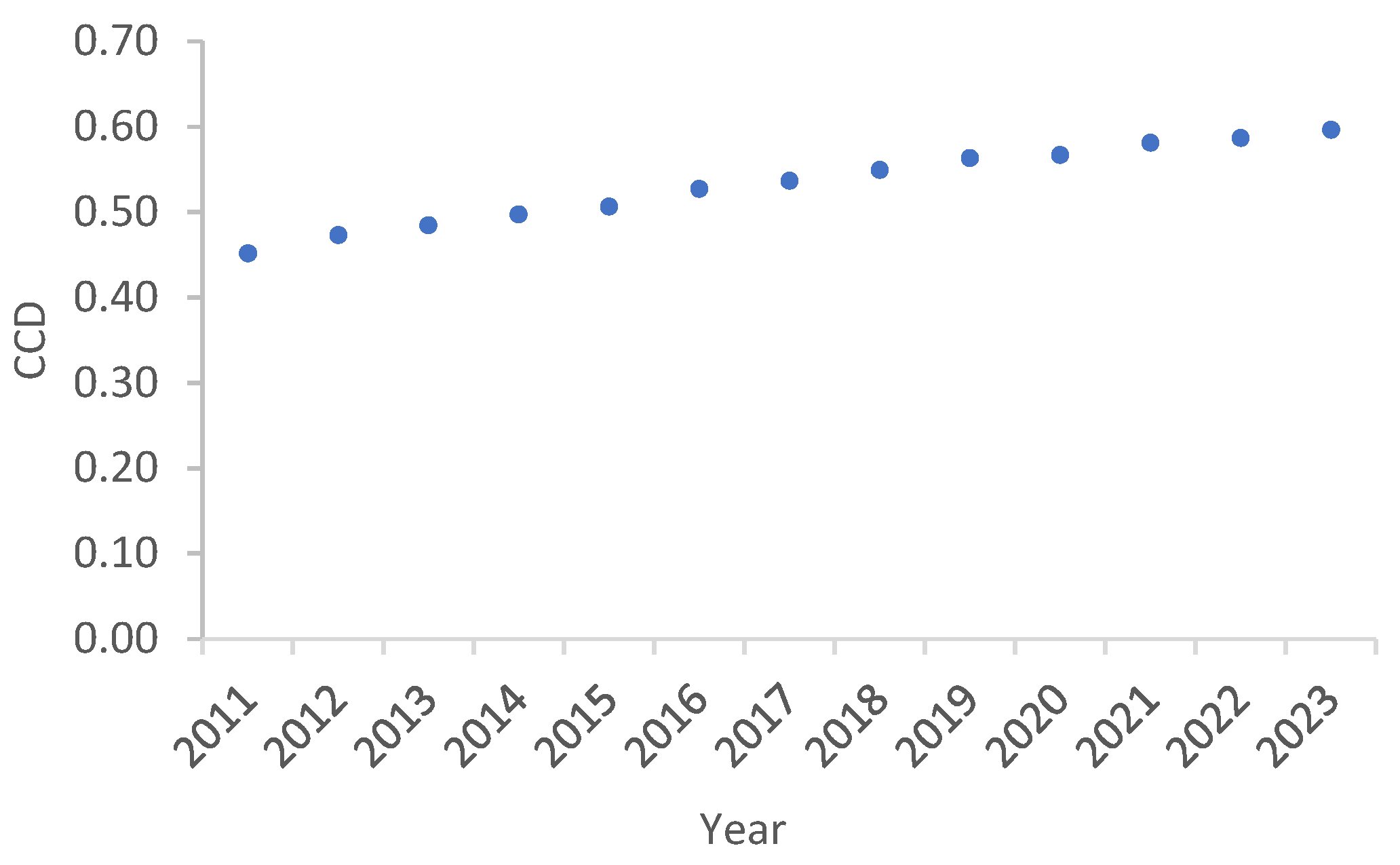
Figure 2 clearly shows D-UEE’s annual increase. According to the classification in Table 5, D-UEE in 2011 was in near-disorder recession. D-UEE in 2023 gradually evolved into primary coordination. This shows that U-EE promotes itself and develops in a coordinated manner.
From 2011 to 2013, the urbanization and ecological environment coordination degree (D-UEE) increased slowly from 0.45 to 0.48. The whole is in a phase of near-disorder recession. The level of coordination in this period was low and failed to form a good momentum of coordinated development. It may be that the scale expansion of the urbanization process has caused some pressure on the ecological elements such as land resources and water resources, while the ecological environment governance capacity and supporting infrastructure construction are relatively lagging behind, resulting in an unstable coupling relationship within the system. From 2014 to 2022, D-UEE continued to rise from 0.50 to 0.59, which was in the stage of reluctance coordination. This stage is a stage of steady improvement of the coordination degree, and the coordination level has achieved a significant leap, indicating that the urbanization system and the ecological environment system have gradually entered the track of coordinated development. This may be due to the comprehensive promotion of the national ecological civilization construction strategy and the implementation of local green development policies [76]. The quality of urbanization has been gradually improved, the industrial structure has begun to transform to low-carbon, and the ecological environment governance has been strengthened, which has eased the conflict between the urbanization system and the ecological environment system. D-UEE in 2023 was further increased to 0.60, entering the primary coordination stage for the first time. This numerical breakthrough indicates that the coupling relationship between urbanization and ecological environment has achieved substantial improvement, and the system has moved from reluctance coordination to primary coordination. The continuous improvement of the coordination degree indicates that the pressure effect of urbanization on the ecological environment is gradually weakening, while the supporting capacity of the ecosystem is further enhanced with the development of time, and the two have entered a stage of benign interaction.
However, the highest D-UEE level in 2023 is only the primary coordination level, and the overall D-UEE in China’s 30 regions is not high. This may stem from regional disparities in the level of urbanization, as well as differences in ecological environmental protection and air quality, leading to a generally low degree of coupling and coordination. In the following, we will analyze the D-UEE of 30 regions in China from a regional perspective.
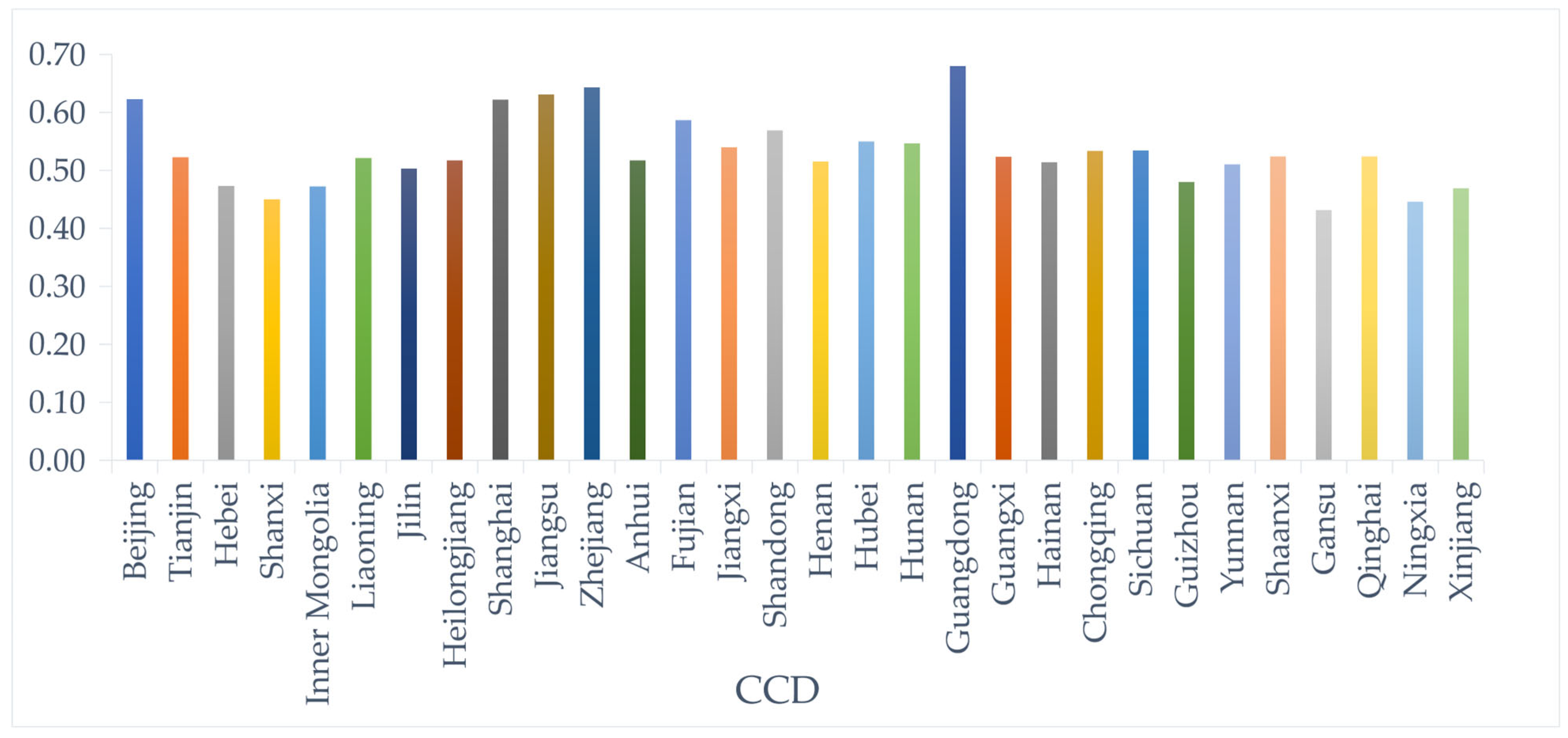
As illustrated in Figure 3, the D-UEE across the 30 regions in China exhibits significant spatial imbalance. For example, Guangdong has the highest D-UEE, followed by Zhejiang, Jiangsu, Beijing, and Shanghai, and the D-UEE of these five regions is greater than 0.6. According to the classification in Table 5, they belong to primary coordination. Gansu has the lowest D-UEE, followed by Ningxia, Shanxi, Xinjiang, Inner Mongolia, Hebei, and Guizhou. The D-UEE of these seven regions is less than 0.5. It belongs to the near-disorder recession. The D-UEE of the other 18 regions is between 0.5 and 0.59, which belongs to reluctance coordination according to the classification in Table 5. It can be concluded that there are large differences in D-UEE across regions. However, further analysis shows that most of the regions with higher D-UEE belong to the eastern region, while most of the regions with lower D-UEE belong to the western region. Thus, it can be concluded that there are regional differences in D-UEE in 30 regions of China. Therefore, we will use the DGID method to further analyze the spatial regional differences in D-UEE.

3.2. DGID Result Analysis

According to the National Bureau of Statistics regional division standards [77,78], the 30 regions of China are divided into four regions, eastern, central, western and northeastern regions, as shown in Table 6.
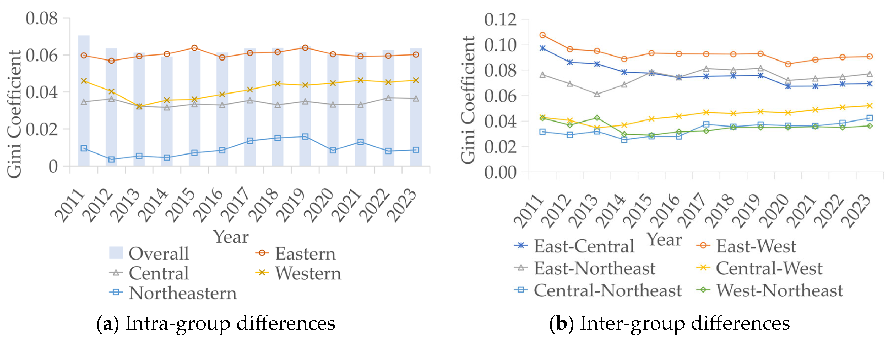
The horizontal axis of Figure 4 represents the study years 2011–2023, and the vertical axis is the Gini coefficient, which indicates the degree of contribution of the difference. Figure 4a shows the overall Gini coefficient of 30 regions and the Gini coefficient of four sub-regions in China from 2011 to 2023, where the blue bars indicate the contribution degree of the overall internal differences in the 30 regions. The four line graphs are eastern, central, western and northeastern regions, respectively, indicating the time series change trend of the differences within the group in different regions. Figure 4b shows the extended Gini coefficient among the four sub-regions from 2011 to 2023. It represents the time series variation trend of differences between different regions.
Figure 4a shows the intra-group differences in the four regions. On the whole, although the intra-group Gini index of D-UEE from 2011 to 2023 exhibits a downward trend, and the overall difference is decreasing year by year, the intra-group Gini index is the highest, and the overall difference is still large. From a regional perspective, the intra-group Gini index was highest in the eastern region among the four regions over the period 2011–2023, indicating significant intra-group disparities. A marked upward fluctuation occurred in 2015, suggesting considerable imbalance in the development of D-UEE within the eastern region. Secondly, in the western region, intra-group disparities decreased significantly in 2013, and then rose steadily on an annual basis beginning in 2013. This indicates that there is a problem of uneven D-UEE development in the western region. In addition, in the central region, the intra-group differences fluctuated little from 2011 to 2023, indicating that the D-UEE difference in the central region remains relatively stable. Last but not least, in the northeastern region, the intra-group differences were relatively small. The intra-group Gini index was relatively low in 2012. After a significant increase in 2019, it decreased significantly again in 2020. This indicates that the development of D-UEE in the northeastern region is relatively balanced.
Figure 4b shows inter-group differences among the four regions, with a total of six different groups. It is evident that the inter-group Gini index for the east–west dimension is the highest, indicating substantial regional disparities between the eastern and western regions. Secondly, the disparity between the east–central regions is relatively large, indicating that the difference between the eastern and central regions is also relatively large. The development of D-UEE in both the east–west and east–central regions has a large imbalance problem. It is worth noting that the east–west and east–central differences are also decreasing year by year. The inter-group Gini index between the east–northeast regions is moderate and also different, indicating that there is also a problem of uneven development of D-UEE. The inter-group Gini indices of the central–west, west–northeast and central–northeast regions are relatively low, indicating only modest disparities; accordingly, the differences are relatively small, and the differences in D-UEE development are relatively balanced.
Table 7 represents the contribution of Gini decomposition to the overall regional disparities in D-UEE development. It is evident that the inter-group difference contributes most substantially to the overall difference, with a mean contrib.-value of 0.039 and a mean contrib.-rate of 62.42%. The intra-group difference has a medium contribution to the overall difference, with an average contrib.-value of 0.014 and an average contrib.-rate of 22.33%. Hypervariable density has the smallest contribution to the overall difference, with an average contrib.-value of 0.010 and an average contrib.-rate of 15.25%. This shows that the reason for the uneven development of D-UEE in the 30 regions of China is mainly due to inter-group differences. Therefore, in order to reduce the imbalance of D-UEE, we should first reduce the differences between different regions, and then pay attention to the differences arising from internal cross-overlap within the region.

3.3. SAM Result Analysis

The GMI results effectively capture the overall spatial distribution characteristics of D-UEE. The value of GMI is [−1, 1]. When GMI is greater than 0, it means that the whole presents the characteristics of clustering, while a value less than 0 indicates overall dispersion. When equal to 0, it indicates that the spatial distribution is random and exhibits no discernible pattern [79].
According to the results in Table 8, from 2011 to 2023, the p-values are all less than 0.01, indicating that GMI is statistically significant at the 99% significance level. The I values are all greater than 0, which is positive, indicating that the D-UEE of the 30 regions in China presents significant spatial clustering distribution characteristics. With the development of time, this spatial clustering feature shows an upward trend as a whole. In terms of numerical values, the global Moran’s I index from 2011 to 2023 is positive, and all of them are between 0.34 and 0.45. Referring to the study of Tsui, T. et al., a value of Moran index close to 1 indicates strong spatial clustering, and 0 indicates the absence of significant clustering [70]. This indicates that there is a significant positive spatial clustering feature in the coupling coordination degree of urbanization and the ecological environment in the study area, but it does not belong to strong clustering. This indicates that there are some random discrete components in the region at the same time, and the spatial structure is not completely highly clustered. This feature reflects that parts of the study area do not strictly follow high–high or low–low clustering pattern.
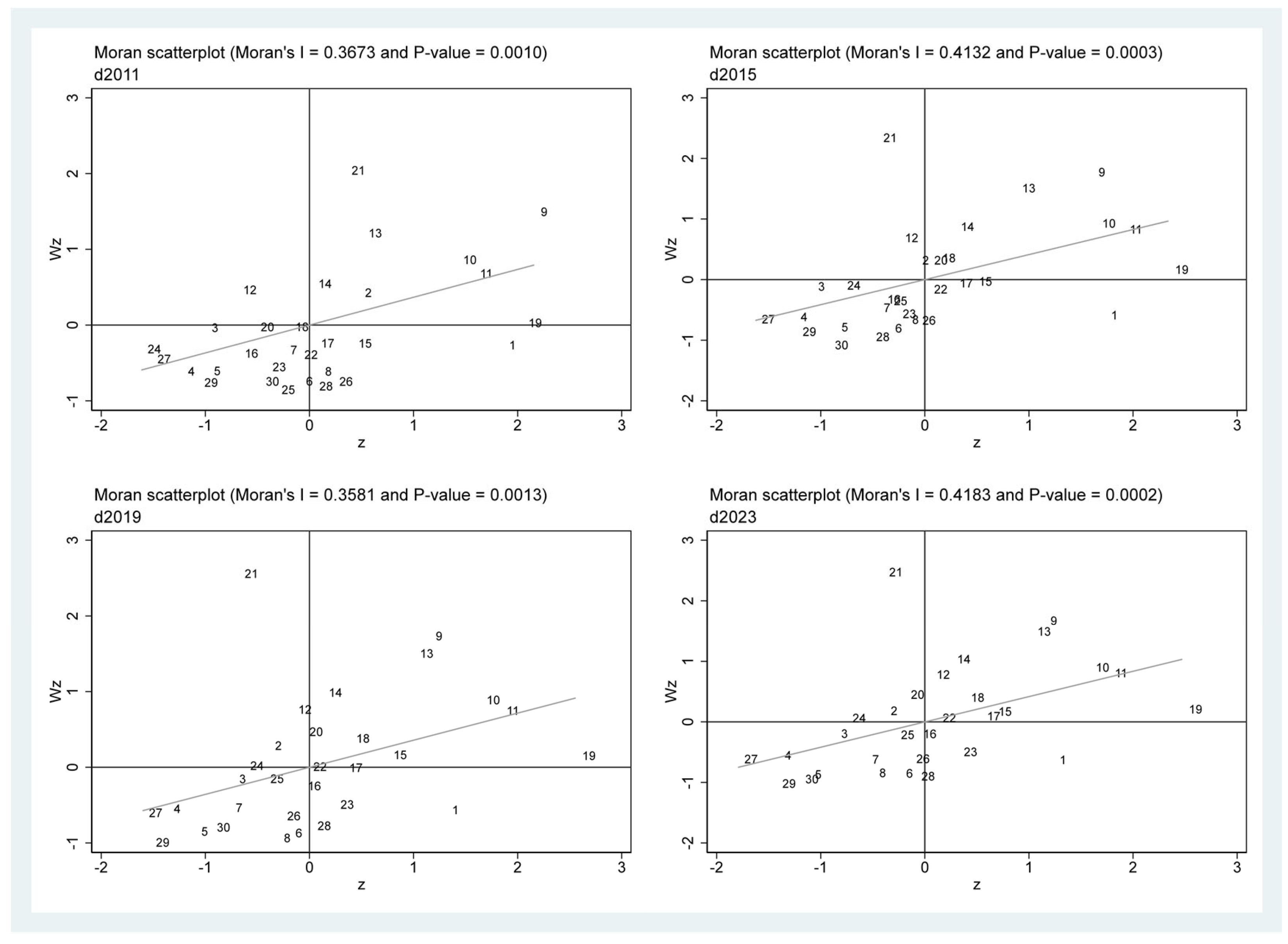
According to GMI, D-UEE is spatially correlated. Therefore, on this basis, the local Moran’s index (LMI) is employed to further investigate the spatial distribution characteristics at the local level. LMI selects the data of the four years 2011, 2015, 2019 and 2023 for analysis. Figure 5 is the LMI scatter plot, where the four quadrants represent distinct types of spatial clustering. The first quadrant is the high–high (HH) type, representing clusters with high D-UEE values. The second quadrant is the low–high (LH) type, which indicates that its own D-UEE value is low and its neighbor’s D-UEE value is high. The third quadrant is the low–low (LL) type, representing clusters of low D-UEE values. The fourth quadrant is the high–low (HL) type, which indicates that its own D-UEE value is high and its neighbor’s D-UEE values are low [65,80]. The numerical numbering in Figure 5 is consistent with Table 6.
According to the results of the LMI scatter plot in Figure 5, on the whole, most regions are in the first and third quadrants in these four years, and a few regions are in the second and fourth quadrants. Most of them belong to HH and LL types, which indicates that most D-UEE values present the distribution characteristics of spatial clustering, and their own D-UEE values are unified with those of their neighbors, with significant positive spatial correlation and strong spatial dependence. A small proportion belongs to LH and HL types, showing the characteristics of null differentiation. The results of the LMI show that not all 30 districts fall within the first and third quadrants. A small number of districts are located in the second and fourth quadrants. This result is consistent with the GMI.
From the perspective of local areas, Shanghai, Jiangsu, Zhejiang, Fujian, Jiangxi and Guangdong have always been in the first quadrant, belonging to the HH type, and most of them are in the eastern region. The nine regions of Hebei, Shanxi, Inner Mongolia, Liaoning, Jilin, Yunnan, Gansu, Ningxia and Xinjiang have always been in the third quadrant, belonging to the LL type, and most of them are in the western region. Both HH and LL types are clusters of the same type. This indicates that the spatial feature of the eastern region is the high-value D-UEE cluster. The spatial feature presented in the western region is the D-UEE low-value cluster. In the second and fourth quadrants, the regions with LH and HL types are relatively few and their distribution is unstable, which indicates that the local spatial negative correlation phenomenon is not obvious. However, a typical HL-type city like Beijing has been in the fourth quadrant in these four years, indicating that Beijing’s own D-UEE is high, while its neighboring cities are low, forming an island-type feature surrounded by low values around it.

3.4. TSA Results Analysis

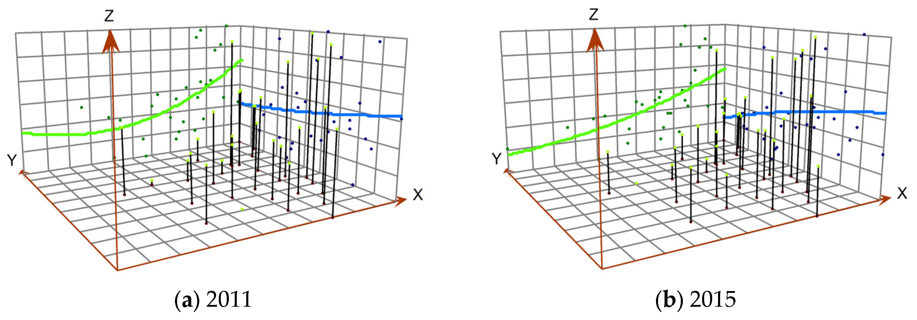
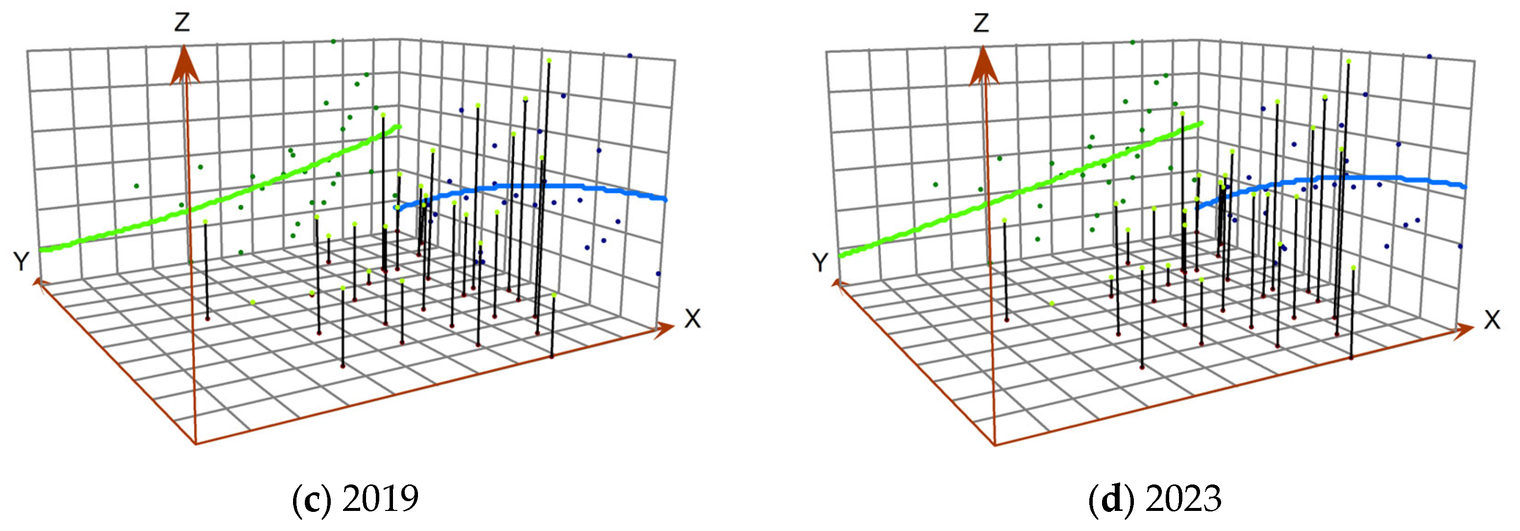
Referring to the study of Wu et al., the trend surface analysis in this study was conducted using ArcMap 10.8 software; the software’s trend surface analysis tool is primarily used to visually illustrate the overall spatial direction and gradient characteristics of the harmony between urbanization and the ecological environment [74]. The TSA selects the data of 2011, 2015, 2019, and 2023 for analysis. In Figure 6, the X-axis represents the east–west direction, and the direction of the X-axis arrow is east; conversely, it is west. The Y-axis represents the north–south direction. The arrow on the Y-axis indicates north, and the opposite direction indicates south. The green curve illustrates the east–west spatial trend of D-UEE across China’s 30 regions. The blue curve shows the spatial trend of D-UEE in the north–south direction.
Figure 6 presents the spatial distribution of D-UEE across the 30 regions. According to the TSA results of the four years in the figure, the overall spatial distribution of D-UEE exhibits a pattern characterized by higher values in the eastern and southern regions and lower values in the western and northern regions. This shows that the eastern and southern regions can maintain the benign interaction between urbanization and the ecological environment well, and the degree of coordinated development between the two is relatively high. However, urbanization development and ecological environmental protection in the western and northern regions exhibit a pronounced contradiction, resulting in a relatively low level of coordination. In terms of spatial division differences, the difference between D-UEE the south and the north is smaller than that between the eastern and western regions. This indicates that the spatial differentiation of D-UEE is mainly dominated by the east–west difference, and the north–south difference is relatively stable. With the development of each region, the spatial difference in D-UEE does not show an obvious trend over time. In contrast, the north–south spatial disparity exhibits a gradual upward trend over the four-year period, reaching its minimum in 2011 and showing a modest increase in the trend from 2015 to 2023. The spatial differences in the east–west direction tended to decrease, with the largest east–west disparity observed in 2011 and a modest decline in the trend from 2019 to 2023.

4. Discussion

4.1. CCD Results Discussion

According to the results of the CCD model, D-UEE is generally low across the 30 regions of China. Further analysis reveals large differences across regions. Generally speaking, the D-UEE is higher in the eastern region and lower in the western region. This may be due to the fact that the eastern region is mainly economically dominated by plains and wetlands, with high vegetation coverage, a good natural environment and strong ecological restoration capacity. However, the western region is ecologically fragile and complex, such as serious soil erosion on the Loess Plateau, serious desertification in the west, and low precipitation. The eastern region has a more obvious advantage in industrial innovation. By the end of 2023, the eastern region had gathered 70.2% of the national equipment manufacturing enterprises above designated size [81]. However, the total assets of industrial enterprises above designated size in the central and western regions rose by 47.7% compared with those at the end of 2018. Although the central and western regions were also growing year by year, the total amount was still low. At present, the urbanization rate in the eastern region, such as Shanghai, Beijing, and Tianjin, has exceeded 85% [82]. Therefore, the D-UEE is higher in the eastern than in the western region.

4.2. DGID Results Discussion

According to the results of DGID, it is found that among the intra-group differences, the overall D-UEE differences in the four regions are decreasing year by year. Among them, the eastern region exhibits the largest disparity, followed by the western and central regions, and the northeastern region has the smallest difference. Among the inter-group differences, east–west differences are the largest. This is followed by the east–central and east–northeast differences. The differences between center–west, west–northeast, and center–northeast are smaller. As the eastern region includes Beijing, Shanghai and other developed areas, with a large number of talents, advanced technology and high-end service industry, the GDP also ranks first in China. However, the eastern region also includes Hebei and Hainan, and there is a big gap between the urbanization quality and industrial base of Beijing and Shanghai. The central and western regions are dominated by traditional manufacturing industries, and their economic development is backward. The northeastern region has a single industrial structure, dominated by heavy industry and agriculture, with a small gap between industries and relatively stable overall urbanization development. Therefore, intra-group variation in the eastern region exceeds that in other regions, and east–west inter-group variation is higher than between other regions.

4.3. SAM Results Discussion

According to the results of the GMI and LMI, a significant positive spatial relationship was found for D-UEE. The local spatial distribution characteristics of most areas belong to the HH type and LL type. This distribution feature indicates that D-UEE shows a distribution pattern of similar clustering. The HH type is mainly in the cities in the eastern coastal areas (such as Shanghai, Jiangsu, Zhejiang, Fujian, Guangdong and other regions). Such areas rank among the top in medical care, education, residents’ income, and public infrastructure in China, and have a good ecological foundation, forming a cluster area with a high D-UEE value. The LL type is mainly in cities in the western region (such as Inner Mongolia, Gansu, Ningxia and Xinjiang). Such areas are relatively backward in terms of medical care, education and residents’ income nationwide, with a poor ecological foundation and a lack of natural resources, so they form the clustering areas with low D-UEE values.

4.4. TSA Results Discussion

According to the TSA results, D-UEE is higher in the eastern regions than in the western regions and higher in the southern regions than in the northern regions across the 30 study regions. Due to the good economic foundation of the eastern and southern regions, the natural conditions are superior, while the western region is more mountainous and arid with less rain. Because of heavy industry and chemical industry in the north, urbanization has greater ecological pressure. Therefore, the D-UEE is higher in the eastern and southern regions than in the western and northern regions. In terms of the characteristics of spatial differences, the north–south difference in D-UEE is smaller than the east–west difference. The east–west disparity is more pronounced, likely attributable to the western region’s scarcity of natural resources and its ecologically fragile environment. Typical regions, such as Xinjiang, Qinghai, Gansu and Yinchuan, are areas with serious drought and desertification. In contrast, the eastern region has high urbanization quality, abundant natural resources, and sufficient investment in technology and environmental protection. Typical regions include Shanghai, Beijing, Guangdong and Fujian. This leads to a sharp difference between the eastern and western regions. North–south differences also exist, but the magnitude of the difference is small, so the magnitude of the impact on D-UEE is weaker than the east–west gap.

5. Conclusions

Based on the panel data of 30 regions in China, the U-EE is comprehensively evaluated. Through the CCD model, the D-UEE level is measured, and it is found that the overall coordination degree is not high, and the regional differences are large. The eastern region has the highest D-UEE, and it is the high-value region of the overall regional pattern. The central and northeastern regions are between the eastern and western regions, which are the median regions of the region as a whole. The western region is the lowest, which is the low-value region of the overall regional pattern. On this basis, the spatial distribution characteristics of D-UEE were further analyzed. Firstly, DGID analysis reveals a year-on-year decline in intra-group differences across the four regions, among which the eastern region exhibits the largest disparity, whereas the northeastern region shows the smallest. Among the inter-group differences, the east–west difference is the largest, and the center–northeast difference is the smallest. Then, using SAM, from a global point of view, D-UEE has a positive autocorrelation phenomenon. Locally, most of the areas are concentrated in the first and third quadrants, corresponding to the spatial distribution types of HH and LL. From the local results, D-UEE exhibits spatial distribution characteristics of high-value and low-value clusters within homogenous clusters. Finally, using TSA, it is found that D-UEE is higher in the eastern and southern regions than in the western and northern regions, and the difference between the eastern and the western regions is large and the difference between the northern and the southern regions is small.
Based on the above research results, it is evident that the differences in D-UEE between regions are mainly dominated by the differences between the eastern and western regions, while the differences between the northern and the southern regions are not obvious. Through the research, it is found that there are spatial differences in the coordinated development between the U-EE systems. The D-UEE level has a strong dependence on space. In particular, it has a great impact on the ecological environment. For example, the eastern coastal and southern areas have natural geographical advantages, sufficient natural resources and very high environmental quality. But in the western region, on the contrary, land desertification is serious and natural resources are scarce. Therefore, we can implement corresponding ecological protection and support policies, promote cleaner production technology more, strengthen forest ecological restoration, strictly control pollutant discharge, and utilize other ways to improve the ecological environment quality in the western and northern regions from various considerations. On the basis of stabilizing economic growth, the ecological environment should be improved, so as to promote the overall coordinated development of regional urbanization and ecological environment.
The Monte Carlo sensitivity analysis in this study is mainly applied to test the stability and fluctuation range of indicator weights under random parameter disturbance, aiming to verify whether the weighting results are robust to minor numerical changes. However, this method only focuses on numerical stability verification within the given indicator system and fixed sample range. It cannot further explain the theoretical rationality of a single indicator’s high weight, nor can it eliminate the inherent bias caused by the original index selection and data structure. Therefore, the analysis results only serve as a robustness auxiliary reference, rather than a complete judgment on the rationality of the entire weighting system. The CCD model is used to quantify the interactive relationship between urbanization and ecological environment. Nevertheless, it is necessary to acknowledge the inherent interpretive boundaries of the CCD model. Firstly, the CCD model is effective in measuring the static coupling level and coordination status of subsystems within a specific time and regional scope, but it has limited capacity to capture the complex dynamic evolutionary mechanism and nonlinear causal pathways behind subsystem interactions. Secondly, the evaluation results of the CCD model are inevitably constrained by the established indicator framework and weight allocation scheme; the model can only provide interpretation based on the selected indicators, and cannot fully cover all latent influencing factors that affect U-EE interactions. Thirdly, the CCD model focuses on reflecting the overall coordination degree of the system, and it is difficult to independently isolate and quantify the marginal contribution and dominant effect of a single indicator (such as per capita water resources) to the whole coupling system. Therefore, the model’s analytical conclusions should be regarded as a macro comprehensive evaluation reference, rather than an absolute interpretation of all micro driving mechanisms and individual indicator rationality. Due to the lack of forecasting models, the practical application of the research results and the ability to predict trends are inevitably limited.
For ecological environment-related indicators, in addition to traditional statistical data, remote sensing observation, geographic monitoring, ground penetration radar (GPR), artificial intelligence (AI/ML) and other technologies have been widely used in natural resource management and ecological environment monitoring [16]. They can effectively improve the objectivity and spatial accuracy of index observation, especially for the western region where statistical data are relatively weak. This study takes statistical data as the core for analysis, and the accuracy of data is limited to some extent. Urbanization policy, climate change and industrial structure all affect the coordinated development of urbanization and ecological environment, but the action path of each factor is complex and intertwined; this is also one of the research limitations of this research. In the future, remote sensing data and intelligent algorithms will be integrated to realize complementary verification of statistical data and spatial monitoring data and improve the reliability of data collection. And we will further expand the research perspective, introduce spatial econometric methods such as the spatial Durbin model (SDM), improve the explanatory variable system, and systematically identify the direct effects of each factor.

Author Contributions

Conceptualization, Q.P.; data curation, Q.P.; investigation, Y.S.; resources, Q.P. and Y.S.; methodology, Q.P. and Y.S.; formal analysis, Q.P. and Y.S.; software, Q.P. and Y.S.; writing—original draft preparation, Q.P. and Y.S.; supervision, Y.S.; validation, Q.P.; visualization, Q.P.; funding acquisition, Y.S. All authors have read and agreed to the published version of the manuscript.

Funding

This research was funded by the Doctoral Research Initiation Fund (DRIF) of Lanzhou Institute of Technology, grant number: 2024 YJ-06.

Institutional Review Board Statement

Not applicable.

Informed Consent Statement

Not applicable.

Data Availability Statement

The original data presented in the study are openly available in the China Statistical Yearbook of the National Bureau of Statistics at https://www.stats.gov.cn/sj/ndsj/ (accessed on 26 January 2025).

Acknowledgments

We would like to thank the institutes who offered funds for this research, and we would also like to thank the anonymous reviewers and editors for commenting on this paper.

Conflicts of Interest

The authors declare no conflicts of interest.

References

  1. National Bureau of Statistics: The Decline in the Total Population Has Narrowed and the Quality of The Population Has Continued to Improve. Available online: https://www.stats.gov.cn/sj/sjjd/202501/t20250117_1958337.html (accessed on 3 February 2025).
  2. Mcintyre, N.E.; Knowles-Yánez, K.; Hope, D. Urban ecology as an interdisciplinary field: Differences in the use of “urban” between the social and natural sciences. Urban Ecosyst. 2000, 4, 5–24. [Google Scholar] [CrossRef]
  3. Young, R.F. Interdisciplinary foundations of urban ecology. Urban Ecosyst. 2009, 12, 311–331. [Google Scholar] [CrossRef]
  4. Douglas, I. Urban ecology and urban ecosystems: Understanding the links to human health and well-being. Curr. Opin. Environ. Sustain. 2012, 4, 385–392. [Google Scholar] [CrossRef]
  5. Kattel, G.R.; Elkadi, H.; Meikle, H. Developing a complementary framework for urban ecology. Urban For. Urban Green. 2013, 12, 498–508. [Google Scholar] [CrossRef]
  6. Ramalho, C.E.; Hobbs, R.J. Time for a change: Dynamic urban ecology. Trends Ecol. Evol. 2012, 27, 179–188. [Google Scholar] [CrossRef] [PubMed]
  7. Wu, J.; Xiang, W.N.; Zhao, J. Urban ecology in China: Historical developments and future directions. Landsc. Urban Plan. 2014, 125, 222–233. [Google Scholar] [CrossRef]
  8. Lawrence, R.J. Human ecology in the context of urbanization. In Integrating Human Health into Urban and Transport Planning, A Framework; Springer International Publishing: Cham, Switzerland, 2018; pp. 89–109. [Google Scholar] [CrossRef]
  9. Tanner, C.J.; Adler, F.R.; Grimm, N.B.; Groffman, P.M.; Levin, S.A.; Munshi-South, J.; Pataki, D.E.; Pavao-Zuckerman, M.; Wilson, W.G. Urban ecology: Advancing science and society. Front. Ecol. Environ. 2014, 12, 574–581. [Google Scholar] [CrossRef]
  10. Wang, Z.; Liang, L.; Sun, Z.; Wang, X. Spatiotemporal differentiation and the factors influencing urbanization and ecological environment synergistic effects within the Beijing-Tianjin-Hebei urban agglomeration. J. Environ. Manag. 2019, 243, 227–239. [Google Scholar] [CrossRef]
  11. Nathaniel, S.P. Natural resources, urbanisation, economic growth and the ecological footprint in South Africa: The moderating role of human capital. Quaest. Geogr. 2021, 40, 63–76. [Google Scholar] [CrossRef]
  12. Shi, C.; Zhu, X.; Wu, H.; Li, Z. Assessment of urban ecological resilience and its influencing factors: A case study of the Beijing-Tianjin-Hebei urban agglomeration of China. Land 2022, 11, 921. [Google Scholar] [CrossRef]
  13. Wang, L.; Qu, Z.; Yang, W.; Ren, E.; Tang, T. Coupled urbanisation and ecological protection along the Yellow river basin in the context of dual carbon. Sustainability 2023, 15, 5728. [Google Scholar] [CrossRef]
  14. Das, M.; Das, A.; Mandal, A. Exploring the factors affecting urban ecological risk: A case from an Indian mega metropolitan region. Geosci. Front 2023, 14, 101488. [Google Scholar] [CrossRef]
  15. Zhang, M.; Ren, Y.; Zhou, L. Spatiotemporal evolution characteristics and influencing factors of urban ecological resilience in the Yellow River Basin. Arid Land Geogr. 2024, 47, 445–454. [Google Scholar] [CrossRef]
  16. Didmanidze, O.N.; Karelina, M.Y.; Klyuev, R.V.; Martyushev, N.V.; Serdechnyy, D.V. Application of artificial intelligence and modern technologies in geomonitoring to improve the efficiency of the mining industry utilising the earth’s resources. News Natl. Acad. Sci. Repub. Kazakhstan Ser. Geol. Tech. Sci. 2025, 2, 84–96. [Google Scholar] [CrossRef]
  17. Yao, J.; Xu, P.; Huang, Z. Impact of urbanization on ecological efficiency in China: An empirical analysis based on provincial panel data. Ecol. Indic. 2021, 129, 107827. [Google Scholar] [CrossRef]
  18. Yang, M.; Jiao, M.; Zhang, J. Coupling coordination and interactive response analysis of ecological environment and urban resilience in the Yangtze River Economic Belt. Int. J. Environ. Res. Public Health 2022, 19, 11988. [Google Scholar] [CrossRef]
  19. Chen, R.; Chen, Y.; Lyulyov, O.; Pimonenko, T. Interplay of urbanization and ecological environment: Coordinated development and drivers. Land 2023, 12, 1459. [Google Scholar] [CrossRef]
  20. National Bureau of Statistics. New Urbanization—A Powerful Engine for Economic and Social Development. Available online: https://www.stats.gov.cn/sj/sjjd/202302/t20230202_1896895.html (accessed on 13 April 2026).
  21. National Bureau of Statistics. Government Information Publicity. Available online: https://www.stats.gov.cn/xxgk/jytadf2020/rddbjy2020/201708/t20170801_1758322.html (accessed on 13 April 2026).
  22. Zou, C.; Zhu, J.; Lou, K.; Yang, L. Coupling coordination and spatiotemporal heterogeneity between urbanization and ecological environment in Shaanxi Province, China. Ecol. Indic. 2022, 141, 109152. [Google Scholar] [CrossRef]
  23. Liu, J.; Tian, Y.; Huang, K.; Yi, T. Spatial-temporal differentiation of the coupling coordinated development of regional energy-economy-ecology system: A case study of the Yangtze River Economic Belt. Ecol. Indic. 2021, 124, 107394. [Google Scholar] [CrossRef]
  24. Peng, B.; Huang, Q.; Elahi, E.; Wei, G. Ecological environment vulnerability and driving force of Yangtze River urban agglomeration. Sustainability 2019, 11, 6623. [Google Scholar] [CrossRef]
  25. Fan, Y.; Fang, C.; Zhang, Q. Coupling coordinated development between social economy and ecological environment in Chinese provincial capital cities-assessment and policy implications. J. Clean. Prod. 2019, 229, 289–298. [Google Scholar] [CrossRef]
  26. Ji, J.; Wang, S.; Zhou, Y.; Liu, W.; Wang, L. Spatiotemporal change and coordinated development analysis of “population-society-economy-resource-ecology-environment” in the jing-jin-ji urban agglomeration from 2000 to 2015. Sustainability 2021, 13, 4075. [Google Scholar] [CrossRef]
  27. Craney, T.A.; Surles, J.G. Model-dependent variance inflation factor cutoff values. Qual. Eng. 2002, 14, 391–403. [Google Scholar] [CrossRef]
  28. Covington, T.R.; Gearhart, J.M. Sensitivity and Monte Carlo analysis techniques and their use in uncertainty, variability, and population analysis. In Physiologically Based Pharmacokinetic (PBPK) Modeling; Academic Press: Cambridge, MA, USA, 2020; pp. 211–242. [Google Scholar] [CrossRef]
  29. Barton, H.A.; Chiu, W.A.; Setzer, R.W.; Andersen, M.E.; Bailer, A.J.; Bois, F.Y.; DeWoskin, R.S.; Hays, S.; Johanson, G.; Jones, N.; et al. Characterizing uncertainty and variability in physiologically based pharmacokinetic models: State of the science and needs for research and implementation. Toxicol. Sci. 2007, 99, 395–402. [Google Scholar] [CrossRef]
  30. Wang, Y.; Cao, Z.; Au, S.K. Efficient Monte Carlo simulation of parameter sensitivity in probabilistic slope stability analysis. Comput. Geotech. 2010, 37, 1015–1022. [Google Scholar] [CrossRef]
  31. Zhe, W.; Xigang, X.; Feng, Y. An abnormal phenomenon in entropy weight method in the dynamic evaluation of water quality index. Ecol. Indic. 2021, 131, 108137. [Google Scholar] [CrossRef]
  32. Xie, T.; Wang, M.; Su, C.; Chen, W. Evaluation of the natural attenuation capacity of urban residential soils with ecosystem-service performance index (EPX) and entropy-weight methods. Environ. Pollut. 2018, 238, 222–229. [Google Scholar] [CrossRef] [PubMed]
  33. Yao, L.; Li, X.; Li, Q.; Wang, J. Temporal and spatial changes in coupling and coordinating degree of new urbanization and ecological-environmental stress in China. Sustainability 2019, 11, 1171. [Google Scholar] [CrossRef]
  34. Wang, Q.; Yuan, X.; Zhang, J.; Gao, Y.; Hong, J.; Zuo, J.; Liu, W. Assessment of the sustainable development capacity with the entropy weight coefficient method. Sustainability 2015, 7, 13542–13563. [Google Scholar] [CrossRef]
  35. Wu, R.M.; Zhang, Z.; Yan, W.; Fan, J.; Gou, J.; Liu, B.; Gide, E.; Soar, J.; Shen, B.; Fazal-e-Hasan, S.; et al. A comparative analysis of the principal component analysis and entropy weight methods to establish the indexing measurement. PLoS ONE 2022, 17, e0262261. [Google Scholar] [CrossRef] [PubMed]
  36. Zhang, X.; Wang, C.; Li, E.; Xu, C. Assessment Model of Ecoenvironmental Vulnerability Based on Improved Entropy Weight Method. Sci. World J. 2014, 2014, 797814. [Google Scholar] [CrossRef]
  37. Wang, X.; Yang, Z. Application of fuzzy optimization model based on entropy weight method in atmospheric quality evaluation: A case study of Zhejiang province, China. Sustainability 2019, 11, 2143. [Google Scholar] [CrossRef]
  38. Stanković, J.J.; Popović, Ž.; Marjanović, I. Assessing smartness and urban development of the European cities: An integrated approach of Entropy and VIKOR. In Multiple Criteria Decision Making: Beyond the Information Age; Springer International Publishing: Cham, Switzerland, 2021; Volume 25, pp. 69–97. [Google Scholar] [CrossRef]
  39. Li, J.; Liu, H.; Xu, J.; Wei, W. Research on Urban Vitality and Development Potential based on Entropy Weight Method. In Proceedings of the 2021 IEEE 6th International Conference on Cloud Computing and Big Data Analytics (ICCCBDA), Chengdu, China, 24–26 April 2021; pp. 6–11. [Google Scholar] [CrossRef]
  40. Deng, W.; Li, X.; Guo, Y.; Huang, J.; Zhang, L. Ecological Assessment of Water Environment in Huizhou Region of China Based on DPSIR Theory and Entropy Weight TOPSIS Model. Water 2024, 16, 2579. [Google Scholar] [CrossRef]
  41. Li, X. TOPSIS model with entropy weight for eco geological environmental carrying capacity assessment. Microprocess. Microsyst. 2021, 82, 103805. [Google Scholar] [CrossRef]
  42. Luo, X.; Luan, W.; Li, Y.; Xiong, T. Coupling coordination analysis of urbanization and the ecological environment based on urban functional zones. Front. Public Health 2023, 11, 1111044. [Google Scholar] [CrossRef] [PubMed]
  43. Sun, C.; Zhang, S.; Song, C.; Xu, J.; Fan, F. Investigation of dynamic coupling coordination between urbanization and the eco-environment—A case study in the Pearl river delta area. Land 2021, 10, 190. [Google Scholar] [CrossRef]
  44. He, J.; Wang, S.; Liu, Y.; Ma, H.; Liu, Q. Examining the relationship between urbanization and the eco-environment using a coupling analysis: Case study of Shanghai, China. Ecol. Indic. 2017, 77, 185–193. [Google Scholar] [CrossRef]
  45. Shang, Y.; Liu, S. Spatial-Temporal Coupling Coordination Relationship between Urbanization and Green Development in the Coastal Cities of China. Sustainability 2021, 13, 5339. [Google Scholar] [CrossRef]
  46. Ye, S.; Wei, C.; Wang, Z. Coupling coordination between resource and environmental carrying capacity and social development quality and its influence mechanism. Ecol. Indic. 2025, 179, 114151. [Google Scholar] [CrossRef]
  47. Zhai, X.; Li, X.; Hong, J.; Shao, Z.; Li, X.; Cao, H. Spatiotemporal Evolution, Influencing Factors and Convergence of the Coupling Coordination Between High-Quality Development and High-Level Protection in Jiangsu, China. Land 2026, 15, 227. [Google Scholar] [CrossRef]
  48. Hou, C.; Chen, H.; Long, R. Coupling and coordination of China’s economy, ecological environment and health from a green production perspective. Int. J. Environ. Sci. Technol. 2022, 19, 4087–4106. [Google Scholar] [CrossRef]
  49. Liu, L.; Wang, X.; Meng, X.; Cai, Y. The coupling and coordination between food production security and agricultural ecological protection in main food-producing areas of China. Ecol. Indic. 2023, 154, 110785. [Google Scholar] [CrossRef]
  50. Ma, T.; Liu, Y.; Yang, M. Spatial-temporal heterogeneity for commercial building carbon emissions in China: Based the Dagum Gini Coefficient. Sustainability 2022, 14, 5243. [Google Scholar] [CrossRef]
  51. Zhou, R.; Jin, J.; Cui, Y.; Ning, S.; Zhou, L.; Zhang, L.; Wu, C.; Zhou, Y. Spatial Equilibrium Evaluation of Regional Water Resources Carrying Capacity Based on Dynamic Weight Method and Dagum Gini Coefficient. Front. Earth Sci. 2022, 9, 790349. [Google Scholar] [CrossRef]
  52. Yan, M.; Wu, J.; Jiang, H.; Kou, Y.; Zhao, W. Comprehensive vulnerability assessment of power system nodes with wind power based on Dagum-Gini coefficient approach. Sci. Rep. 2025, 15, 11597. [Google Scholar] [CrossRef]
  53. Zhang, L.; Ma, X.; Ock, Y.S.; Qing, L. Research on regional differences and influencing factors of Chinese industrial green technology innovation efficiency based on dagum gini coefficient decomposition. Land 2022, 11, 122. [Google Scholar] [CrossRef]
  54. Hong, H.; Liao, H.; Li, T.; Yang, J.; Xie, D. Analysis of spatio-temporal patterns of rural space function based on entropy value method and Dagum Gini coefficient. Trans. Chin. Soc. Agric. Eng. 2016, 32, 240–248. [Google Scholar] [CrossRef]
  55. Monti, M.G. A Note on the Dagum Decomposition of the Gini Inequality Index; Working Paper n. 2007-16; Dipartimento di Scienze Economiche Aziendali e Statistiche, Universita’degli Studi di Milano: Milan, Italy, 2007; pp. 1–18. [Google Scholar]
  56. Dagum, C. A new approach to the decomposition of the Gini income inequality ratio. Empir. Econ. 1997, 22, 515–531. [Google Scholar] [CrossRef]
  57. Mussard, S. The bidimensional decomposition of the Gini ratio. A case study: Italy. Appl. Econ. Lett. 2004, 11, 503–505. [Google Scholar] [CrossRef]
  58. Griffith, D.A. Extreme eigenfunctions of adjacency matrices for planar graphs employed in spatial analyses. Linear Algebra Its Appl. 2004, 388, 201–219. [Google Scholar] [CrossRef]
  59. Janatabadi, F.; Ermagun, A. Access weight matrix: A place and mobility infused spatial weight matrix. Geogr. Anal. 2024, 56, 746–767. [Google Scholar] [CrossRef]
  60. Yin, F.; Qian, Y.; Zeng, J.; Wei, X. The spatial spillover effects of transportation infrastructure on regional economic growth—An empirical study at the provincial level in China. Sustainability 2024, 16, 8689. [Google Scholar] [CrossRef]
  61. Noglo, Y.A.; Ouedraogo, N.K. Using Dagum’s Gini decomposition to assess households’ asset-based gap in the regions of Burkina Faso. Econ. Bull. 2020, 40, 2241–2253. [Google Scholar]
  62. Cheng, Y.; Zhang, Y.; Wang, J.; Jiang, J. The impact of the urban digital economy on China’s carbon intensity: Spatial spillover and mediating effect. Resour. Conserv. Recycl. 2023, 189, 106762. [Google Scholar] [CrossRef]
  63. Sun, J.; Chen, C.; Sun, Z. Urban economic resilience and its influencing factors in the Yellow River Basin: From the perspective of different types of city. Econ. Geogr. 2022, 42, 1–10. [Google Scholar] [CrossRef]
  64. Chen, T.J.; Chuang, K.S.; Wu, J.; Chen, S.C.; Hwang, I.M.; Jan, M.L. A novel image quality index using Moran I statistics. Phys. Med. Biol. 2003, 48, N131–N137. [Google Scholar] [CrossRef] [PubMed]
  65. Bai, Y.; Deng, X.; Jiang, S.; Zhang, Q.; Wang, Z. Exploring the relationship between urbanization and urban eco-efficiency: Evidence from prefecture-level cities in China. J. Clean. Prod. 2018, 195, 1487–1496. [Google Scholar] [CrossRef]
  66. Liu, Y.; Hu, Z.; Li, Y. Process and cause of urban-rural development transformation in the Bohai Rim Region, China. J. Geogr. Sci. 2014, 24, 1147–1160. [Google Scholar] [CrossRef]
  67. Chen, Y. An analytical process of spatial autocorrelation functions based on Moran’s index. PLoS ONE 2021, 16, e0249589. [Google Scholar] [CrossRef]
  68. Wang, Z.; Fang, C. Spatial-temporal characteristics and determinants of PM2.5 in the Bohai Rim Urban Agglomeration. Chemosphere 2016, 148, 148–162. [Google Scholar] [CrossRef]
  69. Fan, C.; Myint, S. A comparison of spatial autocorrelation indices and landscape metrics in measuring urban landscape fragmentation. Landsc. Urban Plan. 2014, 121, 117–128. [Google Scholar] [CrossRef]
  70. Tsui, T.; Derumigny, A.; Peck, D.; Van Timmeren, A.; Wandl, A. Spatial clustering of waste reuse in a circular economy: A spatial autocorrelation analysis on locations of waste reuse in the Netherlands using global and local Moran’s I. Front. Built Environ. 2022, 8, 954642. [Google Scholar] [CrossRef]
  71. Liu, H.; Guo, P.; Liu, J.; Liu, R.; Tong, T. An extension of multiquadric method based on trend analysis for surface construction. IEEE J. Sel. Top. Appl. Earth Obs. Remote Sens. 2023, 16, 3435–3441. [Google Scholar] [CrossRef]
  72. Bai, X.J.; Kang, H.X.; Wang, P.X.; Liu, Z. Effectiveness of upscaling the vegetation temperature condition index retrieved from Landsat data using an algorithm combining the trend surface analysis and the spatial variation weight method. Eur. J. Remote Sens. 2021, 54, 29–41. [Google Scholar] [CrossRef]
  73. Guo, B.; Pei, T.; Song, C.; Shu, H.; Wu, M.; Guo, S.; Jiang, J.; Du, P. Trend surface analysis of geographic flows. Int. J. Geogr. Inf. Sci. 2023, 37, 118–137. [Google Scholar] [CrossRef]
  74. Wu, N.; Wu, J. Spatiotemporal Evolution and Pathways for Enhancing Urban Competitiveness in China. Land 2026, 15, 161. [Google Scholar] [CrossRef]
  75. Wang, H.; Zuo, R. A comparative study of trend surface analysis and spectrum–area multifractal model to identify geochemical anomalies. J. Geochem. Explor. 2015, 155, 84–90. [Google Scholar] [CrossRef]
  76. National Bureau of Statistics. The 24th in the Series of Achievements in Economic and Social Development Since the 18th CPC National Congress. Available online: https://www.stats.gov.cn/zt_18555/ztfx/18fzcj/index_1.html (accessed on 13 April 2026).
  77. National Bureau of Statistics. China’s Manufacturing Purchasing Managers’ Index Was 50.8 Percent in May 2013. Available online: https://www.stats.gov.cn/sj/zxfb/202302/t20230203_1898306.html (accessed on 6 June 2025).
  78. National Bureau of Statistics. The Pattern of Development Takes on a New Look. Available online: https://www.stats.gov.cn/zt_18555/ztfx/ggkf40n/202302/t20230209_1902596.html (accessed on 7 June 2025).
  79. Lian, Y.; Fan, J.; Lu, C. A Study on the Spatio-Temporal Evolution Characteristics of Social Development Levels in China. Land 2024, 13, 565. [Google Scholar] [CrossRef]
  80. Chen, Y. New approaches for calculating Moran’s index of spatial autocorrelation. PLoS ONE 2013, 8, e68336. [Google Scholar] [CrossRef]
  81. National Bureau of Statistics. The Results of the Fifth National Economic Census Show That China’s Industrial Economy Continues to Grow and the New Driving Force Is Thriving. Available online: https://www.stats.gov.cn/sj/sjjd/202502/t20250227_1958812.html (accessed on 3 August 2025).
  82. National Bureau of Statistics. How to Calculate the Urbanization Rate of Permanent Resident Population. Available online: https://www.stats.gov.cn/zs/tjws/tjzb/202301/t20230101_1903783.html (accessed on 4 August 2025).
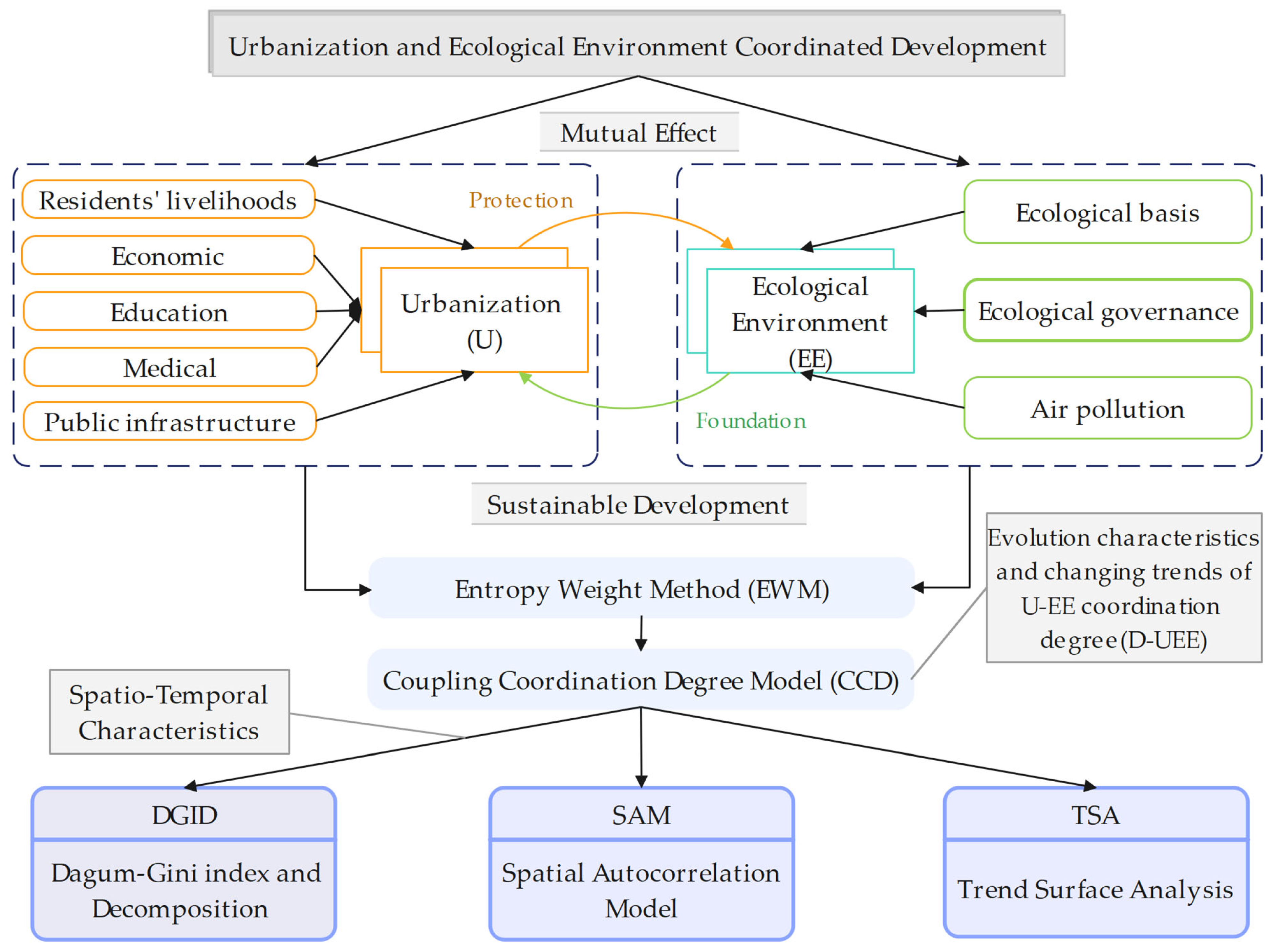
Figure 1. U-EE structural framework.
Sustainability 18 04559 g001
Figure 2. D-UEE (time perspective).
Sustainability 18 04559 g002
Figure 3. D-UEE (regional perspective).
Sustainability 18 04559 g003
Figure 4. Regional DGID.
Sustainability 18 04559 g004
Figure 5. LMI results.
Sustainability 18 04559 g005
Figure 6. TSA results.
Sustainability 18 04559 g006aSustainability 18 04559 g006b
Table 1. VIF test (urbanization indicators).
SubsystemVariablesVIF1/VIF
UPer Capita Regional GDP7.580.13
HCIHTP per 1000 Persons5.330.19
TIAV/Regional GDP3.540.28
PLC Per Person3.330.30
HEE per 100,000 Population2.430.41
HCIB per 1000 Persons2.220.45
PCAPR2.020.49
PCPRGS1.940.52
CGTRS1.860.54
UAPD1.410.71
Mean VIF3.17-
Table 2. VIF test (ecological and environmental indicators).
SubsystemVariablesVIF1/VIF
EESO2 Emission2.65 0.38
PM Emission2.39 0.42
DGCTV1.80 0.56
COD Emission1.62 0.62
BDGCR1.58 0.63
ISWIRR1.57 0.64
PCWR1.31 0.77
FCR1.25 0.80
Mean VIF1.77-
Table 3. Indicator system for U-EE.
SubsystemDimensionVariablesUnitWeightDirection
UResidents’ livelihoodsUAPDPersons/Sq.km0.071+
RPCDIYuan0.113+
CGTRS100 Million Yuan0.182+
EconomicPer Capita Regional GDPYuan0.116+
TIAV/Regional GDP %0.064+
EducationPLC Per PersonCopy0.181+
HEE per 100,000 Population Person0.065+
MedicalHCIB per 1000 PersonsBeds0.054+
HCIHTP per 1000 PersonsPerson0.052+
Public infrastructurePCAPRSq.m0.050+
PCPRGSSq.m0.053+
EEEcological basisBDGCR%0.028 +
PCWRCu.m/Person0.308 +
FCR%0.122 +
Ecological governance ISWIRR%0.077 +
CSDDC10,000 Cu.m0.197 +
DGCTV10,000 Tons0.178 +
Air pollutionPM Emission10,000 Tons0.016
COD EmissionTons0.052
SO2 Emission10,000 Tons0.023
Note: All data utilized in this study are drawn from the China Statistical Yearbook.
Table 4. U-EE weight stability test (running a Monte Carlo simulation 50 times).
SubsystemVariablesEWM-WeightMC-WeightCV
UUAPD0.0710.0710.012
RPCDI0.1130.1130.025
CGTRS0.1820.1820.008
Per Capita Regional GDP0.1160.1160.013
TIAV/Regional GDP0.0640.0650.047
PLC Per Person0.1810.1800.013
HEE per 100,000 Population0.0650.0660.023
HCIB per 1000 Persons0.0540.0540.026
HCIHTP per 1000 Persons0.0520.0520.024
PCAPR0.050.0490.012
PCPRGS0.0530.0530.032
EEBDGCR0.0280.0290.085
PCWR0.3080.3080.005
FCR0.1220.1210.006
ISWIRR0.0770.0770.026
CSDDC0.1970.1960.005
DGCTV0.1780.1780.005
PM Emission0.0160.0160.046
COD Emission0.0520.0520.056
SO2 Emission0.0230.0230.044
Table 5. CCD classification.
D-ValueCoordination Level
0.00–0.09Extreme disorder recession
0.10–0.19Serious disorder recession
0.20–0.29Moderate disorder recession
0.30–0.39Light disorder recession
0.40–0.49Near-disorder recession
0.50–0.59Reluctance coordination
0.60–0.69Primary coordination
0.70–0.79Middle coordination
0.80–0.89Well coordination
0.90–1.00High coordination
Table 6. Four regional classifications.
RegionalRegions
Eastern1. Beijing, 2. Tianjin, 3. Hebei, 9. Shanghai, 10. Jiangsu, 11. Zhejiang, 13. Fujian, 15. Shandong, 19. Guangdong, 21. Hainan
Central4. Shanxi, 12. Anhui, 14. Jiangxi, 16. Henan, 17. Hubei, 18. Hunan
Western5. Inner Mongolia, 20. Guangxi, 22. Chongqing, 23. Sichuan, 24. Guizhou, 25. Yunnan, 26. Shaanxi, 27. Gansu, 28. Qinghai, 29. Ningxia, 30. Xinjiang
Northeastern6. Liaoning, 7. Jilin, 8. Heilongjiang
Table 7. Contribution of Gini decomposition to overall differences.
YearGwGnbGt
Contrib. ValueContrib. Rate %Contrib. ValueContrib. Rate %Contrib. ValueContrib. Rate %
20110.01520.7170.04767.3810.00811.902
20120.01321.1590.04165.0010.00913.840
20130.01320.5560.04167.2950.00712.149
20140.01322.2710.03762.4180.00915.311
20150.01422.1020.03963.2700.00914.628
20160.01321.8370.04065.4730.00812.689
20170.01422.3320.04062.4890.01015.179
20180.01522.8230.03961.3440.01015.833
20190.01522.9560.03959.7790.01117.264
20200.01423.9280.03457.2810.01118.791
20210.01423.5070.03759.5480.01016.945
20220.01423.0750.03860.4850.01016.440
20230.01523.0680.03859.6930.01117.240
mean0.01422.3330.03962.4200.01015.247
Table 8. GMI results.
YearIZp
20110.36733.27970.0010
20120.41813.67670.0002
20130.36813.28170.0010
20140.34793.12420.0018
20150.41323.65990.0003
20160.40863.62260.0003
20170.38703.44640.0006
20180.34613.12000.0018
20190.35813.21970.0013
20200.39403.51360.0004
20210.40923.63470.0003
20220.45494.00740.0001
20230.41833.70140.0002
Disclaimer/Publisher’s Note: The statements, opinions and data contained in all publications are solely those of the individual author(s) and contributor(s) and not of MDPI and/or the editor(s). MDPI and/or the editor(s) disclaim responsibility for any injury to people or property resulting from any ideas, methods, instructions or products referred to in the content.