Article

The Low-Carbon Efficiency Illusion in Agricultural and Rural Systems: Efficiency Measurement, Threshold Effects, and Sustainable Mitigation Strategies


College of Economics and Management, Xinjiang Agricultural University, Urumqi 830000, China
*
Author to whom correspondence should be addressed.
Sustainability 2026, 18(9), 4299; https://doi.org/10.3390/su18094299
Submission received: 23 March 2026 / Revised: 21 April 2026 / Accepted: 24 April 2026 / Published: 26 April 2026

Abstract

This study examines agricultural and rural carbon emission efficiency and the underlying “low-carbon efficiency illusion” in China, where measured efficiency gains fail to translate into genuine environmental improvements. Using panel data from 30 Chinese provinces spanning 2000 to 2022, this study employs a meta-frontier slack-based measure (SBM) model to assess agricultural and rural carbon emission efficiency across meta-frontier and group-frontier benchmarks and investigates the efficiency illusion from the perspective of carbon emission reduction cost constraints. We further combine the Extreme Gradient Boosting (XGBoost) model and Shapley Additive Explanations (SHAP) explainability methods to identify core drivers of agricultural carbon emission reduction costs. We find that technical inefficiency is the primary constraint on China’s agricultural and rural carbon emission efficiency; the number of provinces with an efficiency illusion shows an initial increase followed by a decrease between 2005 and 2022; and core drivers of emission reduction costs exhibit heterogeneous impacts and significant threshold effects across the two frontier frameworks. These findings offer evidence-based guidance for designing differentiated, targeted emission reduction strategies to mitigate the efficiency illusion, advance low-carbon agricultural transition, and support the sustainable development of agricultural and rural systems in the context of the United Nations Sustainable Development Goals.

1. Introduction

The global transition toward carbon peaking and carbon neutrality represents a systemic, society-wide transformation essential. Agriculture plays a unique dual role in this context: it must safeguard global food security and inclusive rural development while contributing to emission reductions [1]. To address these challenges, the Chinese government has introduced a range of policies targeting agricultural carbon emission reductions [2], such as the Action Plan for Agricultural and Rural Carbon Reduction and Sequestration. Despite these efforts, existing research reveals a paradox: while agricultural carbon emission efficiency has shown a continuous upward trajectory, the anticipated improvements in environmental quality have not materialized. This disparity has given rise to the phenomenon known as the “low-carbon efficiency illusion”, wherein overly optimistic efficiency estimates conceal the true shortfalls in emission reductions [3]. Such an illusion exacerbates the misalignment between policy expectations and real-world outcomes. In addition, the rural social system—shaped by the urban-rural dual structure—is deeply interconnected with agricultural production practices. This connection underscores the importance of addressing the carbon emissions generated by rural residential energy consumption. Achieving comprehensive progress in agricultural and rural systems requires a synergistic approach that balances economic, social, and environmental benefits, ensuring advancements in productivity, quality, and ecological sustainability. How to reduce the carbon emissions cost associated with economic development is a central issue of sustainable development. Therefore, it is imperative to reconstruct the evaluation framework for agricultural and rural carbon emission efficiency within an integrated and holistic context. This involves identifying the key constraints on efficiency, examining inter-provincial disparities, and devising sustainable strategies to mitigate the efficiency illusion. Ultimately, this study seeks to provide innovative perspectives and practical solutions to inform the precise formulation of emission reduction policies, particularly in the context of developing countries.
Within the academic community, extensive research has been conducted on agricultural and rural carbon emission efficiency, yielding a wealth of findings across various dimensions. These include efficiency evaluation, temporal and spatial dynamics, spatial effects, and the identification of influencing factors. In terms of indicator system development, the dominant framework in existing literature adopts a standard input-output structure: core inputs typically include agricultural capital, land, labor, and production materials, with gross agricultural output as the primary desirable output, and carbon emissions from agricultural production inputs, rice cultivation, and livestock farming as the key undesirable outputs [4,5]. For efficiency estimation, three methodological approaches are widely adopted in the literature: the Slacks-Based Measure (SBM) model accounting for undesirable outputs [6], conventional Data Envelopment Analysis (DEA) [7], and Stochastic Frontier Analysis (SFA) [8]. Following efficiency estimation, existing studies have largely focused on spatiotemporal dynamics and spatial spillover effects, documenting a broad upward trend in agricultural carbon emission efficiency across national and regional scales, alongside significant regional polarization and localized spatial agglomeration [9]. Further scholarship has examined the coupling and coordination between agricultural carbon emission efficiency and economic growth [10], as well as agricultural modernization [11]. Studies have also employed a range of econometric approaches—including linear regression models and geographical detectors—to unpack the drivers of efficiency dynamics, with a particular focus on the impacts of the digital economy [12], urban-rural integration [5], and industrial agglomeration [13]. In the research regarding the carbon emission costs and carbon shadow prices in agriculture and rural areas, scholars have primarily analyzed agricultural pollutants and the shadow prices and pollution costs associated with agricultural water use [14,15]. Some studies have also focused on the impact of agricultural informatization on carbon shadow prices [16], while others have employed non-parametric methods [17] and techniques such as spatial adaptive reference sets to measure agricultural production and carbon shadow prices [18]. Moreover, there is currently a limited amount of research on the phenomenon of carbon emission efficiency illusion in agriculture and rural areas. Only a few studies have explored this topic. For instance, Wang Lianfen et al. [19] introduced the concept of environmental efficiency illusion; however, the input-output relationships in industry and agriculture differ, which may lead to an overestimation of agricultural environmental efficiency. In this context, He Peipei et al. [3] proposed the concept of low-carbon efficiency illusion in agricultural production, suggesting that the number of provinces in China experiencing low-carbon efficiency illusion in agriculture initially increased and then decreased.
Existing research provides a solid theoretical foundation for this study, but certain gaps remain that warrant further exploration: First, the commonly used frameworks for measuring agricultural carbon emission efficiency predominantly focus on three major carbon sources tied to agricultural production—namely, farmland use, material consumption, and livestock and poultry farming—treated as undesirable outputs. However, these frameworks overlook the carbon emissions generated by rural residential energy consumption, which may lead to an overestimation of carbon emission efficiency. Second, current research has largely neglected the heterogeneity of agricultural and rural carbon emission efficiency, making it difficult to pinpoint the underlying causes of efficiency deficits. Studies by Battese et al. [20] have demonstrated that the meta-frontier approach can effectively address efficiency measurement issues under technological heterogeneity, offering a potential solution to this gap. Third, most studies fail to account for the rigid constraints imposed by factor price limitations on the improvement of agricultural and rural carbon emission efficiency. The assumption that faster economic development necessarily leads to higher efficiency may lead to conclusions that do not fully reflect actual conditions, failing to explain the observed discrepancy between high efficiency and environmental quality improvement. Fourth, many empirical studies rely on traditional econometric methods to analyze the degree of influence of various factors. However, traditional econometric models are limited in their ability to handle high-dimensional variables and nonlinear relationships [21], making it challenging to accurately identify multiple influencing factors and conduct threshold analyses.
Unlike previous studies, the present study utilizes panel data from 30 provinces in China spanning the years 2000 to 2022, focusing on the agricultural and rural sectors. When constructing the indicator system for agricultural and rural carbon emission efficiency, we systematically incorporate carbon emissions arising from both agricultural production processes and rural residential energy consumption, which aligns with the full-chain carbon emission characteristics of China’s agricultural and rural sectors. Subsequently, within the framework of the meta-frontier theory, we employ the meta-frontier SBM model to measure the carbon emission efficiency of China’s agricultural and rural sectors. This allows us to calculate the marginal cost of carbon reduction in these areas and to evaluate the phenomenon of low-carbon efficiency illusion from a cost constraint perspective. To further mitigate the emergence of this efficiency illusion, we utilize the Extreme Gradient Boosting (XGBoost) model and Shapley Additive Explanations (SHAP) interpretability methods to explore the influencing factors and thresholds of agricultural and rural carbon reduction costs. This approach helps to deepen the understanding of agricultural and rural carbon reduction and may provide useful implications for the formulation of differentiated carbon reduction policies, providing valuable insights for advancing carbon neutrality.
This study contributes to the literature in three respects: (1) We construct a holistic evaluation framework for agricultural and rural carbon emission efficiency from a full-system perspective, incorporating carbon emissions from rural residential energy consumption into the indicator system, which helps reduce the estimation bias associated with the narrow focus on agricultural production in much of the existing literature; (2) it proposes and measures the concept of agricultural and rural low-carbon efficiency illusion from the perspective of carbon reduction costs, offering an alternative perspective for assessing whether efficiency gains are substantively meaningful; (3) by combining the meta-frontier SBM model with XGBoost-SHAP analysis, the study identifies the nonlinear and heterogeneous effects of key determinants on carbon reduction costs, thereby improving the understanding of regional low-carbon transition pathways.

2. Materials and Methods

2.1. Measurement of Carbon Emission Efficiency in China’s Agriculture and Rural Areas

Using the meta-frontier SBM model and referring to the studies of Ji Ming et al. [22] and Tian Yun et al. [23], this research selects three categories of indicators—inputs, expected outputs, and unexpected outputs—to evaluate agricultural and rural carbon emission efficiency in China. The input indicators include rural fixed asset investment, employment in the primary industry, total sown area of crops, total power of agricultural machinery, and total consumption of agricultural plastic films, fertilizers, and pesticides. Additionally, rural residents’ domestic energy consumption is incorporated as an input indicator, as it constitutes a critical component of the rural carbon emission system and directly contributes to total rural carbon emissions. Neglecting this component would lead to an incomplete representation of the energy inputs driving agricultural and rural carbon emission efficiency. This energy indicator encompasses ten common energy types—raw coal, coke, liquefied petroleum gas, kerosene, gasoline, diesel, fuel oil, natural gas, electricity, and heat—all converted into standard coal equivalents. The desirable output is represented by the total output value of agriculture, forestry, animal husbandry, and fishery. The undesirable output reflects the total carbon emissions from agriculture and rural areas, calculated based on four primary sources: agricultural material inputs, crop cultivation, livestock breeding, and rural domestic energy consumption, with carbon emission coefficients referenced from Wu Xianrong et al. [24]. It is important to note that this study specifically focuses on carbon emission efficiency within the agricultural and rural system. While other environmental externalities, such as agricultural non-point source pollution and soil degradation, are acknowledged as relevant dimensions of agricultural sustainability, they are beyond the defined scope of this study. Future research may consider broadening the framework of unexpected outputs to include these dimensions for a more comprehensive evaluation of agricultural and rural sustainability.
Following the research methodology established by Färe et al. [25], a meta-frontier SBM model was developed to assess the carbon emission efficiency of decision-making units under the assumption of variable returns to scale (VRS). The mathematical expression of the model is as follows:
ρ = min   1 1 M m = 1 M S m o x x m o   1 + 1 Z + J z = 1 z S z o y y z o + j = 1 J S j o b b j o , s . t . x m o = n = 1 N λ n x m n + S m o x ; y z o = n = 1 N λ n y z n S z o y ; b j o = n = 1 N λ n b j n + S j o b ; S m o x 0 , S z o y 0 , S j o b 0 , n = 1 N λ n = 1
In the formula, ρ represents the efficiency value, strictly decreasing and satisfying 0 < ρ 1 . x m o , y z o , b j o individually represent the m input of the o decision-making unit, the z expected output, and the j undesired output. S m o x , S z o y , S j o b represents the slack variable. n = 1 N λ n = 1 represents the VRS constraint. The group-frontier focuses on the D M U within the group. The calculation form is consistent with Equation (1).
Suppose the meta-frontier efficiency is represented by ρ meta , and the group-frontier efficiency is represented by ρ h , then the common technical gap ratio is expressed as TGR = ρ meta / ρ h . It reflects the relative efficiency of the agricultural and rural carbon emissions of the group, as well as the degree of closeness of the agricultural and rural carbon emission efficiencies.
To further investigate improvement strategies for enhancing carbon emission efficiency in agriculture and rural areas across provinces, we adopt the decomposition method proposed by Chiu [26]. This approach breaks down the inefficiency of carbon emissions in agriculture and rural areas into two components: technical inefficiency and management inefficiency. The relationship can be expressed as follows:
ρ T O I = 1 ρ m e t a = ρ T I + ρ M I ρ T I = ρ h × ( 1 T G R ) = ρ h ρ m e t a ρ M I = 1 ρ h
In the formula, ρ T O I represents the overall inefficiency in carbon emissions. ρ T I represent technical inefficiency. ρ M I represents management inefficiency.
By using the Charnes-Cooper transformation, Equation (1) is transformed into a linear programming form:
max u y y o u x x o u b b o s . t . z = 1 z u z y y z o m = 1 M u m x x m o j = 1 J u j b b j o 0 ; u x 1 M 1 / x o ; u y 1 u x x o u b b o + u y y o Z + J 1 / y o ; u b 1 u x x o u b b o + u y y o Z + J 1 / b o
In the formula, Px, Py and Pb represent the input, the factor prices of expected output and unexpected output. Referring to the research of Färe et al. [27], we standardize the shadow price of the expected output to 1. Consequently, the absolute shadow price of the non-expected output factor can be expressed as:
P b = P y × u b u y
Furthermore, the calculation formula for carbon emission reduction costs can be expressed as follows: C t = i = 1 n Q i t P i t . C t represents the cost of agricultural carbon reduction, Q i t represents the agricultural and rural carbon emissions of the i province in the t year, and P i t represents the shadow price of agricultural and rural carbon emissions in the i province in the t year.

2.2. Assessment of the Low-Carbon Efficiency Illusion in China’s Agriculture and Rural Areas

The agricultural and rural low-carbon efficiency illusion belongs to the broader category of environmental efficiency illusions. It refers to a situation in which the nominal value of agricultural and rural low-carbon efficiency increases while actual environmental quality continues to deteriorate, driven by rising carbon emission reduction costs that are obscured by rapid growth in the agricultural and rural economy. This concept should be distinguished from simple efficiency measurement bias: the illusion does not arise from errors in efficiency calculation, but rather from a structural divergence between the growth trajectory of agricultural and rural economic output and the marginal cost of carbon emission reduction, which causes conventional efficiency metrics to overstate genuine low-carbon progress in agricultural and rural systems.
The formation mechanism of this illusion can be understood through three scenarios in which agricultural and rural low-carbon efficiency may nominally improve. In the first scenario, agricultural and rural economic output increases while carbon emissions remain stable or decline—this represents a genuine improvement in both efficiency and environmental quality. In the second scenario, both output and carbon emissions decrease, but emissions fall at a faster rate than output—this also reflects real environmental improvement, albeit accompanied by a contraction in production. The third scenario constitutes the defining condition of the agricultural and rural low-carbon efficiency illusion: both output and carbon emissions increase simultaneously, but emissions grow at a slower rate than output. In this case, low-carbon efficiency improves only in a nominal sense. Carbon emissions from agricultural production and rural daily life continue to rise, the marginal cost of emission reduction increases, and the overall environmental quality of agricultural and rural areas deteriorates, yet the efficiency metric registers an apparent gain.
The fundamental cause of this illusion is that the absolute growth in the agricultural and rural economic level far exceeds the absolute increase in carbon emission reduction costs, masking the widening gap between their respective growth rates. Introducing a price perspective further clarifies the boundary conditions. In the actual operation of agricultural production and rural daily life, rising carbon emissions are consistently accompanied by increasing carbon emission reduction costs [24]. Given a fixed agricultural output price p and a shadow price of agricultural and rural carbon emissions q, low-carbon efficiency is jointly determined by the relationship between economic output and total carbon emissions. When the growth rate of the agricultural and rural economy significantly outpaces the growth rate of carbon emission reduction costs, low-carbon efficiency will continue to rise even in the absence of meaningful emission reductions. This dynamic masks the actual increase in marginal abatement costs and the underlying deterioration of the agricultural and rural environment, ultimately generating the trap of the agricultural and rural low-carbon efficiency illusion.
Building on this theoretical framework and drawing on existing research [3], this study operationalizes the agricultural and rural low-carbon efficiency illusion as the ratio of the growth rate of carbon emission reduction costs to the growth rate of the agricultural and rural economic level, formally expressed as follows:
I t = C t / C t 1 1 V t / V t 1 1
In the formula, I t represents the degree of the illusion of carbon emission efficiency in agriculture and rural areas, C t is the cost of carbon emission reduction in agriculture and rural areas, V t is the economic level, and the specific indicators are expressed by the total output value of agriculture, forestry, animal husbandry, and fishery. When I t > 1 is true, the illusion of carbon emission efficiency in agriculture and rural areas is in the high illusion range; when 0 < I t < 1 is true, it is in the low illusion range; when I t < 0 is false, there is no illusion of carbon emission efficiency in agriculture and rural areas.

2.3. Interpretable Machine Learning Methods

2.3.1. The XGboost Method

XGBoost was proposed by Chen et al. [28] as an improved algorithm based on gradient boosting decision trees. In each iteration, a decision tree is added, and through an additive strategy, a strong learner is continuously optimized. The objective function of the XGBoost algorithm consists of a loss function and a regularization term. The loss function measures the deviation between the predicted values and the actual values, with the goal of optimizing the model by minimizing this loss. The regularization term comprises the number of leaf nodes and the squared sum of the weights of the leaf nodes, serving to control the model’s complexity and prevent overfitting. The optimal objective function of XGBoost can be expressed as follows:
O b j = 1 2 T j = 1 G j 2 H j + λ + γ T
In the formula, λ represents a fixed coefficient. γ denotes a complexity parameter. T indicates the number of leaf nodes in the tree. G j is the sum of the first-order derivatives of the samples contained in leaf node j . H j is the sum of the second-order derivatives of the samples in leaf node j .

2.3.2. Shap Value Method

Shap values were first introduced by L. Shapley in 1953 [29] to address the problem of contribution distribution in cooperative games. Building on this foundation, Lundberg and Lee developed the SHAP framework [30]. The core idea behind SHAP is to measure the contribution of each influencing factor to the model’s prediction by calculating their average marginal contributions when they are added to the model. SHAP values, which represent the Shapley values of individual feature factors, quantify the extent to which these features contribute to the model’s prediction results. The calculation of SHAP values can be expressed with the following formula:
φ i = S N i S ! n S 1 ! n ! f S i f S
In the formula, φ i represents the contribution of the i feature; N denotes the set of all features; S signifies a subset of features used for prediction; S i indicates the model prediction with the inclusion of the i feature, while f S represents the model prediction without this feature.
SHAP employs an additive feature attribution method to generate interpretable models, meaning that the output of the model is defined as a linear combination of the input variables. The specific formula for this linear model can be expressed as follows:
g z = φ 0 + M i = 1 φ i z i
In the formula, z 0 , 1 M indicates a binary vector where each element corresponds to an input feature; it equals 1 when the feature is observed and 0 otherwise. M represents the total number of input features. φ 0 denotes the predicted outcome when no features are considered, also referred to as the base value. φ i represents the Shapley value associated with the i feature, quantifying its contribution to the model’s prediction.
This study combines the XGBoost method from ensemble learning and the SHAP interpretable machine learning method to analyze the influencing factors of the cost of carbon emission reduction in agriculture and rural areas. This approach overcomes the limitation of the XGBoost model, that it cannot explain the contribution of individual factors, multiple factors, and the relationships between factors. It improves the interpretability of the output of machine learning models in nonlinear regression problems and can quantify the average marginal contribution of each influencing factor when added to the model. Then, it explains the “black box model” from both a global and local perspective [31]. However, the complex integrated decision tree model operates within a closed prediction process. SHAP provides a visualization interface that allows for the calculation of the contribution of each feature when it is incorporated into the model. This approach elucidates the relationship between feature variables and the model’s prediction process. Furthermore, through techniques such as SHAP values, factor importance ranking, and feature contribution rates, the influence of individual indicator factors can be effectively visualized. The method is based on Zhou Da Peng et al. [32], Zhao Qiu et al. [33], and Zhang Lei et al. [34].

2.4. Data Source

This study focuses on 30 provincial-level administrative in China, with a study period spanning 2000 to 2022. The Tibet Autonomous Region, Hong Kong, Macao Special Administrative Regions, and Taiwan Province are excluded from the sample due to the long-term unavailability of continuous and complete agricultural and rural carbon emission-related statistical data. As the world’s largest producer and consumer of agricultural products, China has the world’s largest rural population and a long-standing urban-rural dual institutional structure, with extreme heterogeneity in agricultural production models, resource endowments, economic development levels, and low-carbon technology adoption across regions. This makes China’s agricultural and rural low-carbon transition a paradigmatic case for global agricultural climate governance.
In this study, the calculations and analyses of agricultural and rural carbon emission efficiency, shadow prices, carbon emission reduction costs, and their influencing factors were performed using Python 3.11 (64-bit). The primary packages utilized in this analysis included SciPy1.15.3, Pandas2.2.3, NumPy2.4.3, SHAP0.48.0, XGBoost3.0.4, and Matplotlib3.10.6. The regional classification follows the “Strategy and Policies for Regional Coordinated Development” published by the Development Research Center of the State Council of China, which divides 30 provinces into eight regions: (1) Northeast Region, including Heilongjiang, Jilin, Liaoning. (2) Northern Coastal Region, including Beijing, Hebei, Shandong, Tianjin. (3) Eastern Coastal Region, including Jiangsu, Shanghai, Zhejiang. (4) Southern Coastal Region, including Fujian, Guangdong, Hainan. (5) Middle Yellow River Region, including Henan, Inner Mongolia, Shanxi, Shaanxi. (6) Middle Yangtze River Region, including Anhui, Hubei, Hunan, Jiangxi. (7) Greater Southwest Region, including Guangxi, Guizhou, Sichuan, Yunnan, Chongqing. (8) Greater Northwest Region, including Gansu, Ningxia, Qinghai, Xinjiang. It should be noted that while the eight-zone classification substantially reduces cross-group technological heterogeneity, some degree of within-group variation may still exist. Future research could further validate this grouping using likelihood ratio tests or cluster analysis.
The data mainly came from the “China Statistical Yearbook” from 2001 to 2023, the “China Rural Statistical Yearbook”, the “China Energy Statistical Yearbook”, the “China Population and Employment Statistical Yearbook”, and the statistical yearbooks of each province from 2001 to 2023. These yearbooks report data corresponding to the years 2000 to 2022. To facilitate aggregation, all types of greenhouse gases were uniformly converted into standard carbon dioxide statistics, with the carbon dioxide conversion coefficient being 44/12. At the same time, to eliminate the influence of price factors, the variables were deflated using the base year of 2000. Among the original indicator data, missing values are predominantly found in a limited number of province-year observations related to rural residential energy consumption and agricultural fixed asset investment. To address all missing values, we employed a province-level time-trend linear interpolation method. Specifically, for each indicator within each province, we constructed a linear time trend model with the year serving as the primary explanatory variable. Descriptive statistics are shown in Table 1.

3. Results

3.1. Measurement of Carbon Emission Efficiency in China’s Agriculture and Rural Areas

Figure 1 presents the calculated results of China’s agricultural and rural carbon emission efficiency values under both the meta-frontier and the group-frontier from 2000 to 2022. The meta-frontier represents the optimal technical level that all groups can currently achieve and serves as the standard for measuring the absolute values of agricultural and rural carbon emission efficiency. In contrast, the group-frontier reflects the “local optimum” attainable within groups sharing similar technical levels, providing an internal measure of agricultural and rural carbon emission efficiency.
The results indicate that under the meta-frontier, the average annual agricultural and rural carbon emission efficiencies for the eight groups were 0.217, 0.260, 0.420, 0.550, 0.126, 0.187, 0.163, and 0.126, respectively. Significant differences exist among the groups, with agricultural and rural carbon emission efficiency in the southern coastal areas substantially surpassing that of other regions. If the potential optimal production technology is adopted, each group has improvement potential of 0.783, 0.740, 0.580, 0.450, 0.874, 0.813, 0.837, and 0.874, respectively, highlighting a significant opportunity for emission reduction.
From a national perspective, the provinces in China with higher agricultural and rural carbon emission efficiencies are Hainan and Shanghai, both exceeding an average efficiency of 0.5. Conversely, Shanxi and Ningxia exhibit the lowest carbon emission efficiencies, each averaging below 0.1. Under the group-frontier, the average annual agricultural and rural carbon emission efficiencies for the eight groups were 0.905, 0.933, 1.000, 0.802, 0.833, 0.964, 0.866, and 0.935, respectively, indicating that the eastern coastal regions are the most efficient at the current technical level. The agricultural and rural carbon emission efficiencies of the other groups have improvement potentials of 0.095, 0.067, 0.198, 0.167, 0.036, 0.134, and 0.065, respectively. Examining the groups individually, in the northeastern region, Liaoning achieved an average annual carbon emission efficiency of 1, while Heilongjiang had the lowest efficiency at 0.838. In the northern coastal region, Hebei was the only province with an average efficiency below 1, at 0.731. In the eastern coastal region, the average efficiency across provinces was 1. The southern coastal region saw Hainan achieving an average efficiency of 1, whereas Guangdong recorded the lowest efficiency at 0.643. In the middle reaches of the Yellow River, both Henan and Shaanxi reached an average efficiency of 1, with Shanxi showing the greatest potential for emission reduction at an average efficiency of 0.518. In the middle Yangtze River region, only Anhui fell below 1, with an average efficiency of 0.856. In the southwestern region, Guangxi and Sichuan achieved an average efficiency of 1, while Guizhou recorded the lowest efficiency at 0.597. Finally, in the northwest region, both Qinghai and Xinjiang had an average efficiency of 1, with Ningxia displaying the lowest efficiency at 0.757.
The Technology Gap Ratio (TGR) reflects the gap between the current production technology level of a group and the potential optimal production technology level. A higher TGR value indicates that the group’s technology level is closer to the potential optimum, with values ranging from 0 to 1.
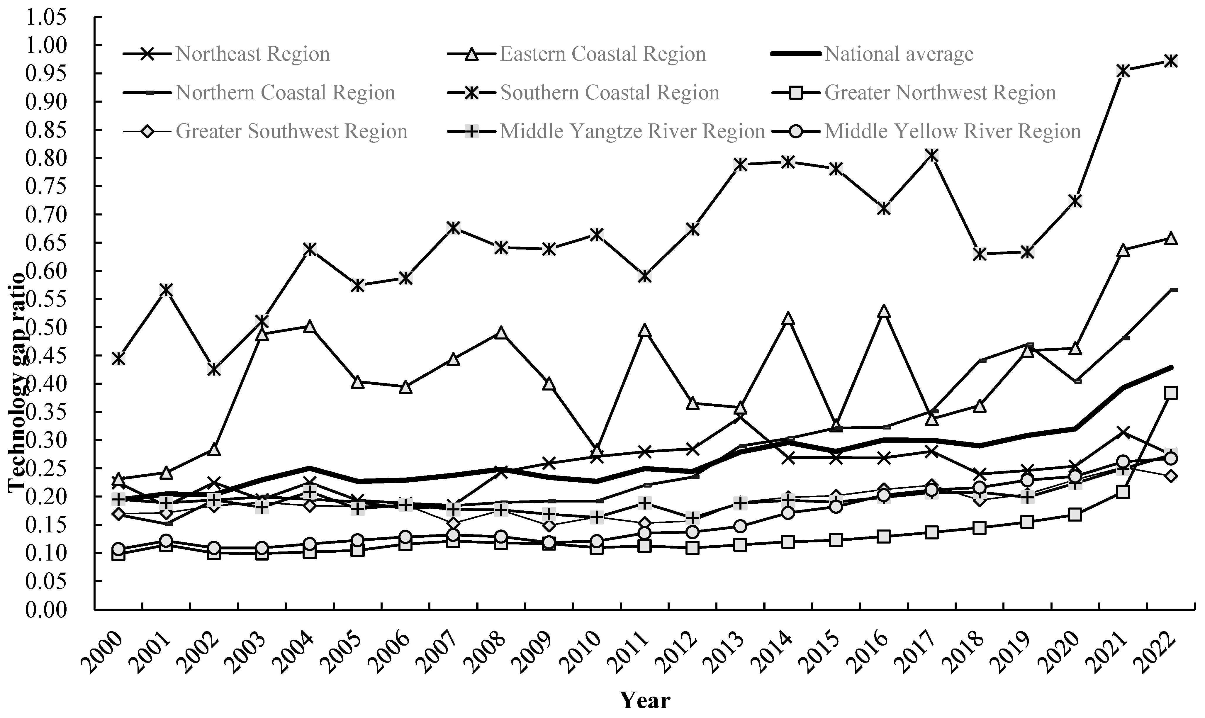
Figure 2 illustrates the average TGR values for eight regions in China from 2000 to 2022. Specifically, the TGR values for the northeastern region, northern coastal region, eastern coastal region, southern coastal region, middle reaches of the Yellow River, middle reaches of the Yangtze River, southwestern region, and northwestern region are 0.248, 0.280, 0.420, 0.671, 0.161, 0.196, 0.189, and 0.135, respectively. A comparison among regions reveals a distinct gradient of TGR values from coastal to inland areas, allowing for the classification into three levels based on proximity to the potential optimal production technology. The first level consists of the southern coastal region, with an average TGR of 0.671, indicating that this area possesses production technology close to the potential optimum. The second level includes the eastern coastal region, the northern coastal region, and the northeastern region, all of which have TGR values above 0.2, with a dominant presence of coastal areas. The third level encompasses the middle reaches of the Yellow River, the middle reaches of the Yangtze River, the southwestern region, and the northwestern region, where TGR values are relatively lower, all below 0.2, suggesting a greater distance from the optimal technology frontier. Notably, the northwestern region has a TGR of only 0.135, indicating the largest technology gap.
From a dynamic perspective, the TGR for all eight regions shows a continuous upward trend, indicating that the agricultural low-carbon technology levels are improving as agricultural modernization progresses. However, the hierarchical structure among regions has not significantly changed. The southern coastal region continues to maintain a technology level above the national average, remaining in a leading position. The eastern coastal and northern coastal regions follow closely behind, exhibiting a fluctuating upward trend and gradually narrowing the gap with the southern coastal region since 2018. The third-level regions consistently remain below the national average TGR, displaying an upward trend but still facing serious technological lag issues. As agricultural economics undergo transformation and technological diffusion continues, it is anticipated that the disparities in TGR among regions will gradually diminish, facilitating the low-carbon transition of the agricultural and rural systems.
To further examine the sources of carbon emission efficiency losses in China’s agricultural and rural areas, Equation (2) is applied to calculate the annual average total inefficiency, technical inefficiency, and managerial inefficiency for 30 provinces over the period 2000–2022. Following the decomposition threshold established by Yan Qingyou et al. [35] provinces are classified according to whether the share of technical inefficiency or managerial inefficiency exceeds 40% of total inefficiency, thereby identifying the dominant direction for efficiency improvement. The results are reported in Table 2.
At the national level, the average total carbon emission efficiency loss is 0.761, indicating substantial room for improvement across China’s agricultural and rural system. Provincial heterogeneity is considerable: 21 provinces, including Jilin, Heilongjiang, and Hebei, record total losses above the national average, while 9 provinces, including Liaoning, Beijing, and Tianjin, fall below it. This dispersion reflects the uneven distribution of low-carbon development capacity across regions.
The decomposition results reveal that technical inefficiency is the dominant source of efficiency loss at the national level, accounting for approximately 87% of total inefficiency on average, with managerial inefficiency contributing the remaining 13%. Notably, 17 of the 30 provinces exhibit group-frontier efficiency values at their maximum, rendering managerial inefficiency structurally zero under the meta-frontier decomposition framework. This pattern is theoretically consistent with the well-documented regional disparities in agricultural technology endowments across Chinese provinces, where the binding constraint on efficiency improvement is access to advanced low-carbon technologies rather than managerial capacity. Consequently, elevating the technological level of low-carbon agricultural production and rural energy use represents the primary pathway for reducing carbon emission efficiency losses across most provinces. Four provinces, namely Shanxi, Fujian, Guangdong, and Guizhou, present a different profile: both technical inefficiency and managerial inefficiency contribute substantially to total efficiency loss, with managerial inefficiency shares exceeding the 40% threshold. These provinces face a dual challenge requiring simultaneous attention to technological upgrading and management improvement.
To verify that this classification is not sensitive to the choice of threshold, we re-examine the provincial groupings using an alternative threshold of 30%. Under this specification, the classification of Shanxi, Fujian, and Guangdong remains unchanged, and Guizhou is additionally identified as requiring management-oriented intervention, representing only a marginal change in the overall pattern. The directional consistency across threshold specifications confirms that technical inefficiency remains the dominant factor.

3.2. Identification of the Illusion of Carbon Emission Efficiency in China’s Agriculture and Rural Areas

Based on the potential deficiencies in the carbon emission efficiency of China’s agricultural and rural sectors during the economic development process, the efficiency illusion values were calculated using Equation (5) for the years 2005, 2010, 2015, 2020, and 2022, as shown in Table 3. Throughout the observation period, the number of provinces exhibiting agricultural and rural low-carbon efficiency illusions under the meta-frontier is consistently higher than those under the group-frontier. This discrepancy arises because the meta-frontier is based on a unified, idealized frontier that overlooks the actual technological disparities among provinces, resulting in many provinces experiencing efficiency illusions. Conversely, the group-frontier is constructed on the basis of the existing technological levels within a group, serving as a more realistic local optimal frontier. Therefore, a focused analysis of efficiency illusions under the group-frontier aligns more closely with actual circumstances. When the efficiency illusion value is less than 1, it indicates that there is no situation where the growth rate of the economic level exceeds the growth rate of carbon reduction costs, leading to an increase in carbon emission efficiency.
Under the group-frontier, the number of provinces in China experiencing agricultural and rural low-carbon efficiency illusions increased from 15 in 2005 to 23 in 2015. However, from 2015 to 2022, this number gradually decreased to 19. Although there is a declining trend in subsequent years, it still suggests that nearly half of the provinces in China have seen an increase in agricultural and rural carbon emission efficiency primarily due to the absolute growth rate of their economic levels exceeding the growth rate of carbon reduction costs, rather than reflecting a genuine low-carbon agricultural and rural production and lifestyle. The increase in carbon emission efficiency is attributed to the declining carbon reduction costs. Specifically, the majority of provinces have efficiency illusion values ranging from 0 to 5, indicating rapid growth in their agricultural economic levels alongside substantial increases in reduction costs. In 2022, the provinces of Anhui, Hunan, Qinghai, Shandong, and Shaanxi reported the highest low-carbon efficiency illusion values, ranking as follows: 127.960, 30.611, 8.754, 8.133, and 6.231. Among them, Anhui Province exhibits a significantly higher efficiency illusion value compared to others, which aligns closely with the actual development trends observed in Anhui’s agricultural and rural sectors in 2022. As one of China’s key grain-producing regions, Anhui’s agricultural economic output demonstrated steady positive growth throughout the year. Concurrently, the large-scale promotion of mature low-carbon agricultural technologies and the accelerated adoption of clean energy in rural households contributed to a notable deceleration in the marginal growth rate of agricultural and rural carbon emission reduction costs in Anhui. This trend accurately reflects the phased development characteristics of the province’s agricultural and rural sectors. These values fall within the high illusion range. suggesting that the growth rate of carbon reduction costs in these provinces significantly exceeds the growth rate of their agricultural economic levels, resulting in negligible improvements in ecological and environmental quality.

3.3. Analysis of the Influencing Factors of Carbon Emission Reduction Costs

3.3.1. Parameter Setting and Model Verification

Based on the previous analysis, the essence of the agricultural and rural low-carbon efficiency illusion lies in the imbalance between the costs of emission reduction and economic growth. Notably, the efficiency illusion can yield negative values, indicating instances where the costs outweigh the benefits. To ensure the robustness of the model, it is essential to investigate the factors that influence changes in emission reduction costs. This exploration can provide targeted pathways for addressing the illusion and enhancing efficiency.
In this study, we focus on the agricultural and rural carbon emission reduction costs under both the meta-frontier and group-frontier frameworks as our target variables. Using the XGBoost model, we allocated 80% of the data for training and the remaining 20% for testing. The model was configured with the following parameters: 500 decision trees, a maximum depth of 4, a feature sampling ratio of 0.8 during node splitting, a sample sampling ratio of 0.8, a minimum node weight of 4, and a learning rate of 0.01. Additionally, L1 and L2 regularization were both set to 1. The results demonstrate that the model performs robustly under both the meta-frontier and group-frontier frameworks. Specifically, for the meta-frontier, the training set achieved an R2 value of 0.908, while the test set attained an R2 of 0.726. In comparison, the group-frontier produced an R2 of 0.834 for the training set, with the test set achieving an R2 of 0.570. These results were further validated through 5-fold cross-validation, confirming that the parameter settings of the model exhibit strong performance on both the training and test sets, characterized by low error rates and significant explanatory power. This indicates that the model is well-calibrated and effective in capturing the underlying relationships influencing agricultural and rural carbon emission reduction costs.

3.3.2. Selection of Influencing Factors

The agricultural ecological environment, as an important part of high-quality development, is influenced by multiple factors including nature, economy, society, and government. Natural development is an unpreventable factor caused by human activities, which directly affects the stability and risk-resistance capacity of agricultural production [36]. This paper selects the degree of land damage to analyze the impact of natural factors on the cost of carbon emission reduction in agriculture and rural areas (Table 4). Economic factors are the core driving force for the development of agriculture and rural areas, and innovative technologies are the key engines for promoting the low-carbon transformation of agriculture [37]. This paper selects the economic development level, rural prosperity level, agricultural industrial structure, and innovation technology level to explore the impact of economic factors on the cost of carbon emission reduction in agriculture and rural areas. Social development cannot be separated from the role of the human subject. By changing the allocation pattern of agricultural resources and improving the acceptance level of agricultural technologies [38], it can indirectly affect the cost of carbon emission reduction in rural areas. This paper selects the rural human capital level and urbanization level to measure the impact of social factors on the cost of carbon emission reduction in rural areas. Policy targeted guidance for the development of agriculture and rural areas provides institutional and financial guarantees [39]. This paper selects the level of fiscal support for agriculture and the level of environmental regulation to measure the impact of government factors on the cost of carbon emission reduction in agriculture and rural areas.

3.3.3. Analysis of Influencing Factors

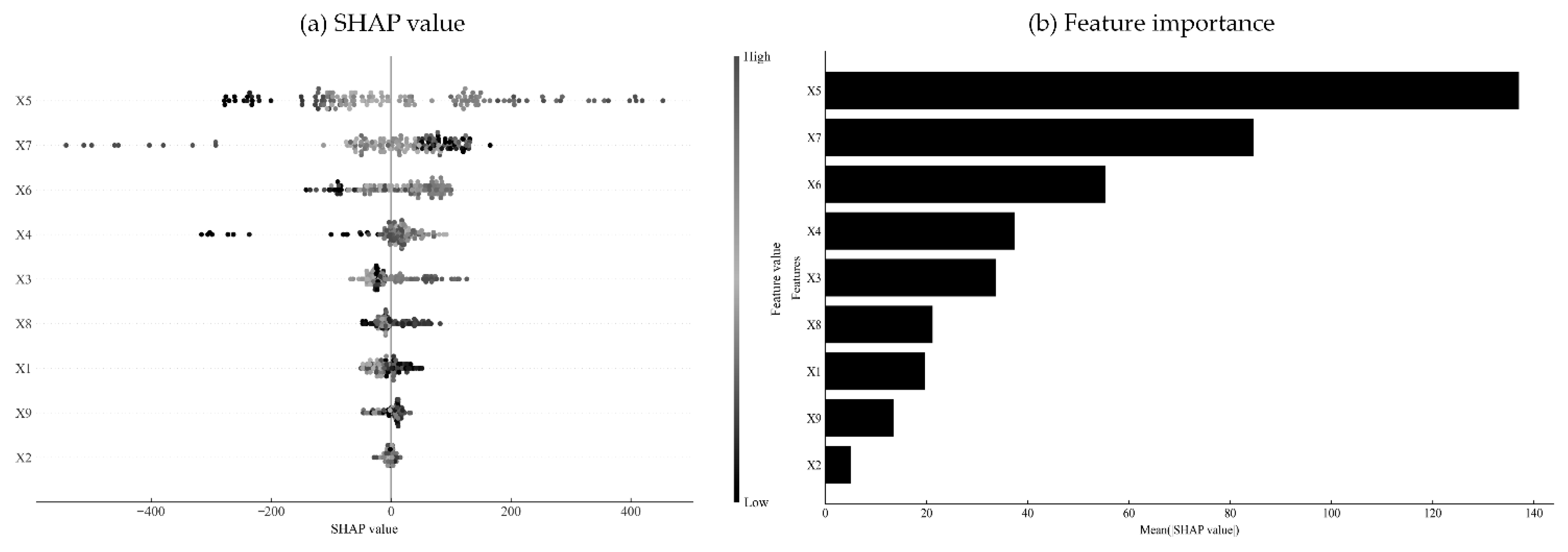
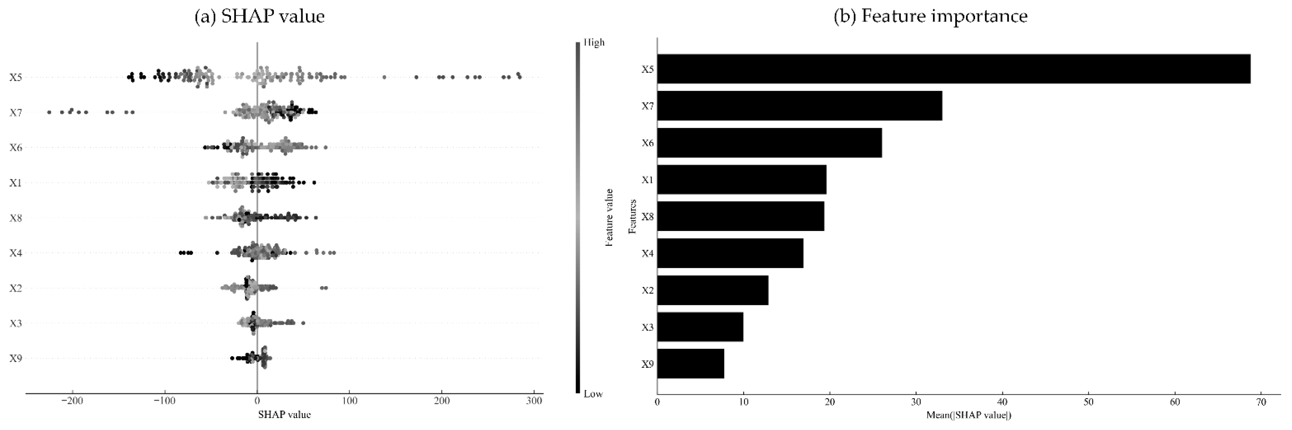
By integrating the SHAP values with the results of the XGBoost model, the positive and negative correlations of the 9 characteristic variables that affect the cost of carbon emission reduction in China’s agriculture and rural areas were analyzed, as shown in Figure 3a and Figure 4a. Under the meta-frontier, the innovation technology level (X5), rural human capital level (X6), and agricultural industrial structure (X4) feature values have a positive correlation with the SHAP contribution; the rural prosperity level (X3) feature value has a weak positive correlation with the SHAP contribution; the urbanization level (X7) feature value has a negative correlation with the SHAP contribution; The eigenvalues of the fiscal support for agriculture level (X8), the degree of land disaster degree (X1), the level of environmental regulation (X9), and the level of economic development (X2) were weakly negatively correlated with the contribution of SHAP. Further analysis shows that Figure 3b indicates that economic and social factors have a significant impact on the carbon emission reduction in China’s agriculture and rural areas. The innovation technology level (X5), urbanization level (X7), rural human capital level (X6), and agricultural industrial structure (X4) are the top four factors in terms of feature importance. Under the group-frontier, the innovation technology level (X5), rural human capital level (X6), agricultural industrial structure (X4), and rural affluence level (X3) feature values have a positive correlation with the SHAP contribution; the urbanization level (X7), land disaster degree (X1), fiscal support for agriculture level (X8), and environmental regulation level (X9) feature values have a negative correlation with the SHAP contribution; the economic development level (X2) feature value has no significant correlation. Further analysis shows that Figure 4b indicates that natural, economic, and social factors have a significant impact on the carbon emission reduction in China’s agriculture and rural areas. The innovation technology level (X5), urbanization level (X7), rural human capital level (X6), and land disaster severity (X1) are the top four factors in terms of feature importance. Based on the above analysis, it can be concluded that whether under the optimal technology level or the existing technology level, economic and social factors are the dominant factors affecting the cost of carbon emission reduction in China’s agriculture and rural areas. Specifically, the influence of the innovation technology level (X5), urbanization level (X7), and rural human capital level (X6) is the greatest.
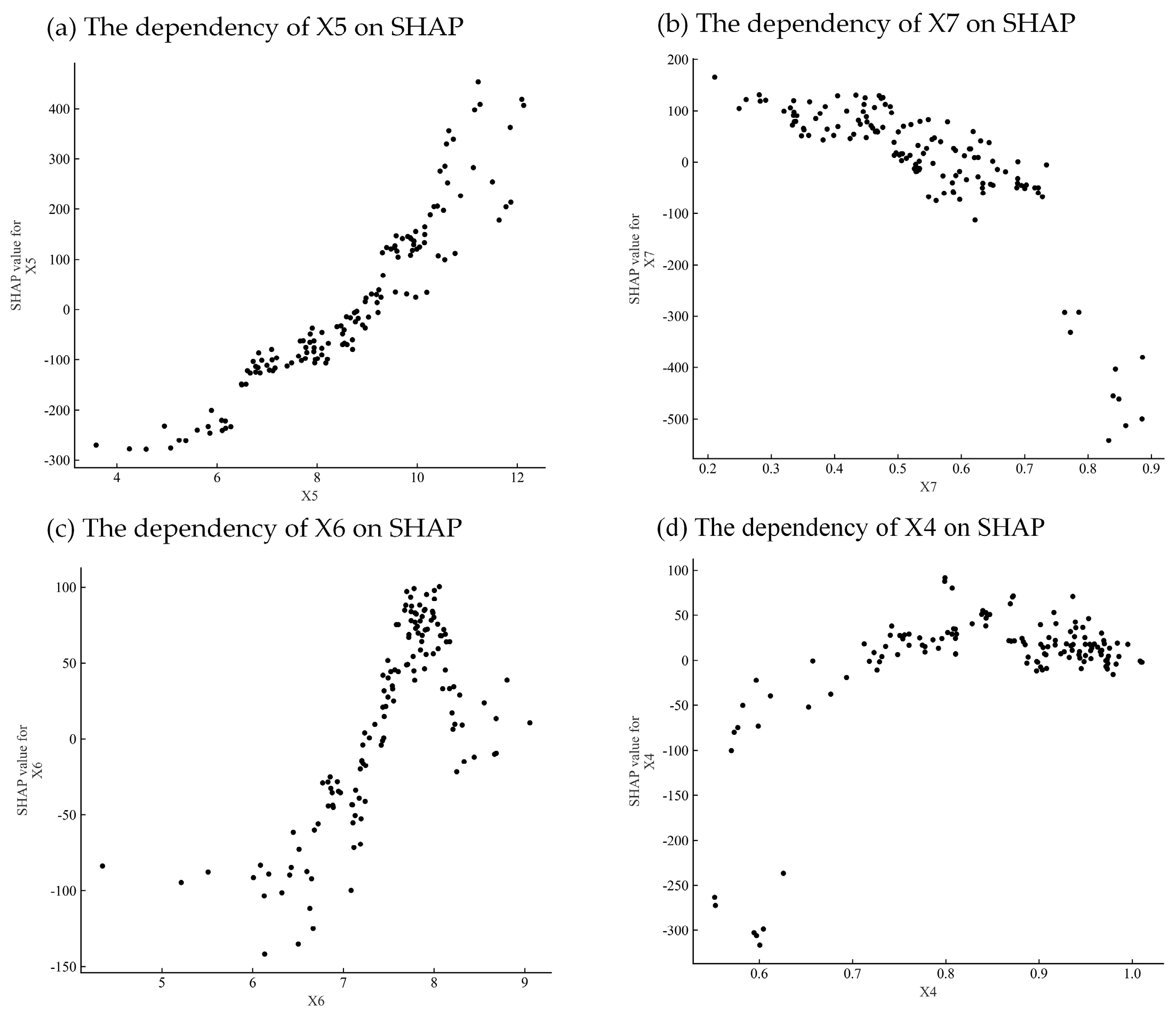
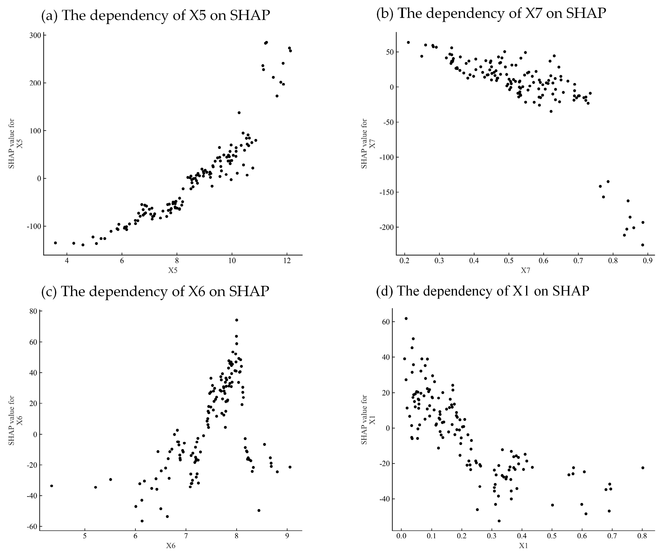
The top four variables in terms of feature importance were selected to construct single-feature SHAP dependence graph (Figure 5 and Figure 6), so as to examine the nonlinear threshold characteristics of individual factors in affecting carbon reduction costs in China’s agricultural and rural sectors. The dependence plots indicate that several key variables exhibit clear turning-point effects, suggesting that their marginal contributions to carbon reduction costs are not constant across the value range, but instead vary with the level of the explanatory variable.
Under the meta-frontier, the innovation technology level (X5) shows a negative SHAP value when its value is below approximately 8, implying that it is associated with lower carbon reduction costs in this range; however, once the value exceeds 8, the SHAP value turns positive and increases rapidly, indicating that the marginal effect shifts toward higher carbon reduction costs. A similar nonlinear pattern is observed for rural human capital (X6). When X6 is below approximately 7, its contribution to carbon reduction costs remains negative; between 7 and 7.5, the SHAP value increases sharply; beyond 7.5, the effect becomes relatively stable at a higher level. For urbanization level (X7), the SHAP value is positive at lower levels and begins to decline substantially once the value exceeds approximately 0.6, suggesting that a sufficiently high urbanization level is associated with a reduction in carbon reduction costs. In contrast, the agricultural industrial structure (X4) exhibits a more gradual threshold effect: when X4 is below 0.7, its SHAP contribution remains negative, whereas values above 0.7 are associated with a gradual increase in carbon reduction costs.
Under the group-frontier, the threshold patterns are broadly consistent but show some differences in turning points. The innovation technology level (X5) remains associated with lower carbon reduction costs when it is below approximately 8.5, while values above 8.5 correspond to a markedly stronger positive contribution. Urbanization level (X7) has a weak cost-increasing effect below approximately 0.45, but once this threshold is crossed, its marginal effect turns sharply cost-reducing. Rural human capital (X6) displays a more complex nonlinear pattern: it slows the growth of carbon reduction costs when below 7.5, increases costs rapidly between 7.5 and 8, and then gradually weakens in its positive effect above 8, eventually tending toward a cost-inhibiting role. Land disaster degree (X1) also exhibits a clear threshold effect: when X1 is below approximately 0.15, it is associated with higher carbon reduction costs, whereas beyond this level, its SHAP value turns negative, indicating a cost-reducing association.
Overall, the SHAP dependence plots reveal that the effects of key determinants are characterized by distinct threshold ranges rather than linear responses. This implies that policy interventions should not only target the direction of influence, but also pay close attention to the specific level at which each factor begins to alter the cost trajectory. Strengthening control over variables near the identified thresholds may help curb the growth of carbon reduction costs and, in turn, alleviate the illusion of agricultural and rural carbon emission efficiency. It should be noted that these threshold values are empirically identified from the SHAP dependence plots and therefore should be interpreted as data-driven turning points rather than strict causal thresholds.

4. Conclusions

This study incorporated rural residential energy use into the carbon accounting framework and applied the meta-frontier SBM model alongside the XGBoost-SHAP method to empirically examine agricultural and rural carbon emission efficiency and the efficiency illusion across 30 Chinese provinces. The following conclusions were obtained:
(1)
Regardless of whether the meta-frontier or the group-frontier is applied, there remains considerable room for improvement in agricultural and rural carbon emission efficiency across China. Significant differences exist among the eight regional groups, with technology gap ratios of 0.248, 0.280, 0.420, 0.671, 0.161, 0.196, 0.189, and 0.135 for the Northeast, Northern Coastal, Eastern Coastal, Southern Coastal, Middle Yellow River, Middle Yangtze River, Southwestern, and Northwestern regions, respectively, revealing a clear coastal-to-inland gradient in technological proximity to the optimal frontier. Efficiency loss decomposition further shows that technical inefficiency is the dominant constraint across all provinces, accounting for approximately 87% of total inefficiency on average, while Shanxi, Fujian, Guangdong, and Guizhou additionally face non-negligible managerial inefficiency. These findings suggest that elevating the level of low-carbon technology adoption and diffusion should be the primary pathway for improving carbon emission efficiency across most provinces, while the four identified provinces additionally require attention to production management capacity, given that both technical and managerial inefficiency contribute substantially to their total efficiency loss.
(2)
Based on the group-frontier, the number of provinces exhibiting agricultural and rural low-carbon efficiency illusion increased from 15 in 2005 to 23 in 2015, before declining to 19 by 2022. For most of these provinces, the apparent rise in carbon emission efficiency was driven by the absolute growth rate of agricultural economic output exceeding the growth rate of carbon reduction costs, rather than reflecting genuine low-carbon transformation. This finding reveals a structural paradox in which measured efficiency improvement can coexist with deteriorating cost conditions, demonstrating that frontier efficiency indicators alone are insufficient to evaluate the quality of the low-carbon transition and that carbon reduction cost dynamics must be explicitly incorporated into the assessment framework.
(3)
The XGBoost-SHAP analysis shows that innovation technology level, urbanization level, and rural human capital level are the most influential determinants of agricultural and rural carbon reduction costs under both frontier settings, followed by agricultural industrial structure under the meta-frontier and land disaster degree under the group-frontier. More importantly, the SHAP dependence plots reveal that each of these factors exhibits clear nonlinear threshold effects and that the critical turning points differ substantially between the meta-frontier and group-frontier specifications. This implies that the same policy instrument may generate different cost consequences depending on the technological reference system and the development stage of a given region, and that effective intervention requires not only identifying the direction of influence but also calibrating policy intensity according to where key variables stand relative to their identified thresholds.

5. Discussion

This study advances the assessment of agricultural and rural low-carbon transition in China by incorporating rural residential energy use into the carbon accounting framework and combining meta-frontier SBM analysis with XGBoost-SHAP interpretation. Compared with conventional studies that focus primarily on agricultural production emissions, this framework captures the joint carbon performance of agricultural production and rural living, thereby providing a more complete picture of carbon emission efficiency and its underlying constraints. More importantly, by introducing carbon reduction costs into the analysis of efficiency illusion, the study reveals that measured efficiency improvement does not necessarily imply substantive low-carbon progress. The integration of frontier analysis and machine-learning-based interpretation therefore helps bridge the gap between static efficiency measurement and the dynamic mechanisms driving low-carbon transition.
The first major finding is that technical inefficiency remains the dominant source of efficiency loss across Chinese provinces, accounting for the overwhelming majority of total inefficiency. This suggests that the central barrier to improving agricultural and rural carbon emission efficiency is not merely the quality of management, but the limited diffusion, absorption, and application of low-carbon technologies. The pronounced coastal-to-inland gradient in technology gap ratios further confirms that technological proximity to the meta-frontier is strongly associated with regional development disparities. Provinces in coastal areas are generally closer to the frontier, whereas inland provinces remain farther behind, indicating that the low-carbon transition is uneven not only in terms of economic development but also in terms of technological access and adaptive capacity. In provinces where technical inefficiency is high, observed gains in efficiency may result more from incremental adjustments or output expansion than from genuine technological upgrading. This means that the apparent narrowing of efficiency gaps should not be interpreted as evidence of substantive low-carbon transformation. For the four provinces where managerial inefficiency is also non-negligible, the implication is that low-carbon transformation depends not only on technological supply but also on the organizational capacity to translate technologies into effective operational outcomes.
A second important contribution of this study is the identification of agricultural and rural low-carbon efficiency illusion. The results show that the number of provinces exhibiting efficiency illusion increased substantially before declining slightly in recent years, suggesting that many provinces experienced rising measured efficiency without a commensurate improvement in carbon reduction conditions. This phenomenon reveals a structural paradox: when economic output grows faster than carbon reduction costs, frontier-based efficiency indicators may improve even if the environmental quality of agricultural and rural development does not. Accordingly, the efficiency illusion should not be regarded as a statistical artifact, but rather as a manifestation of the mismatch between growth-oriented development and emission-reduction constraints. The illusion is particularly informative because it highlights the limitations of conventional frontier measures, which tend to reward output growth while underweighting the cost side of the low-carbon transition. The implication is that the evaluation of agricultural and rural carbon performance should move beyond single-dimensional efficiency scores and explicitly incorporate carbon reduction cost dynamics. In this regard, the use of the group-frontier is especially valuable because it provides a more realistic benchmark for judging whether a province is genuinely improving or merely approaching a locally feasible frontier while still facing rising reduction costs.
The third major finding concerns the nonlinear determinants of carbon reduction costs. The XGBoost-SHAP results show that innovation technology level, urbanization level, and rural human capital level are the most influential factors under both frontier settings, while agricultural industrial structure and land disaster degree also play important roles depending on the frontier specification. What is particularly noteworthy is that these variables exhibit clear threshold effects, and the thresholds differ between the meta-frontier and group-frontier models. This threshold heterogeneity carries substantial policy implications. It indicates that interventions aimed at reducing carbon reduction costs should be sequenced rather than uniformly deployed. For example, when innovation capacity or rural human capital remains below the threshold, additional investment may initially raise adjustment costs because the absorptive capacity required to convert resources into efficiency gains is still weak. Once the threshold is crossed, however, the same factor is more likely to produce cost-saving effects through better technology adoption and more efficient resource allocation. Therefore, policies should be calibrated not only to regional heterogeneity but also to the position of each key determinant relative to its threshold.
Taken together, in formulating low-carbon development policies for the agricultural and rural sectors, adopting the group-frontier as a short-term reference benchmark can help enhance factor allocation efficiency and technological progress, while the meta-frontier should be the long-term strategic goal for substantive low-carbon transformation. It is essential to consider the threshold effects of core determinants on carbon reduction costs and implement targeted policy calibration to slow the growth of agricultural and rural carbon reduction costs. This approach serves as an effective pathway to improving carbon emission efficiency and addressing the efficiency illusion. In the long term, efforts should focus on optimizing the agricultural industrial structure, promoting advanced agricultural production and management technologies, expanding clean energy use in both agricultural production and rural residential life, and improving the agricultural socialized service system. Leveraging the cross-regional diffusion of low-carbon technologies and human capital accumulation can enhance agricultural climate resilience, while improving the efficiency of agricultural resource utilization and advancing standardized large-scale livestock farming are crucial for sustainable cost control. These measures will drive high-quality development and low-carbon green transformation in the agricultural and rural sectors, enabling provincial production systems to converge continuously toward the meta-frontier, and ultimately maintain a balanced synergy between economic and ecological benefits for sustainable growth.

Author Contributions

Conceptualization, Y.X.; methodology, Y.X.; software, Y.X.; validation, Y.X. and X.C.; formal analysis, Y.X. and G.Y.; investigation, Y.X., X.C. and G.Y.; resources, X.C. and G.Y.; data curation, X.C. and G.Y.; writing—original draft preparation, Y.X. and G.Y.; writing—review and editing, Y.X., X.C. and G.Y.; visualization, Y.X., X.C. and G.Y.; supervision, X.C.; project administration, G.Y. All authors have read and agreed to the published version of the manuscript.

Funding

This study was supported by the National Natural Science Foundation of China (72163032).

Institutional Review Board Statement

Not applicable.

Informed Consent Statement

Not applicable.

Data Availability Statement

Restrictions apply to the availability of these data. Data were obtained from national statistical databases and are available from the authors with the permission of national statistical databases.

Conflicts of Interest

The authors declare no conflicts of interest.

Abbreviations

The following abbreviations are used in this manuscript:
XGboostExtreme Gradient Boosting
SHAPShapley Additive Explanations
SBMSlacks-Based Measure

References

  1. Han, J. Prioritizing agricultural, rural development and implementing the rural revitalization strategy. China Agric. Econ. Rev. 2020, 12, 14–19. [Google Scholar] [CrossRef]
  2. Ji, K.; Kong, X.; Leung, C.-K.; Shum, K.-L. Navigating sustainability through environmental regulations: Assessing the effects of command-and-control and market-incentive policies on carbon emissions in China. Sustainability 2025, 17, 2559. [Google Scholar] [CrossRef]
  3. He, P.-P.; Zhang, J.-B.; He, K.; Chen, Z.-K. Why there is a low-carbon efficiency illusion in agricultural production: Evidence from Chinese provincial panel data in 1997–2016. J. Nat. Resour. 2020, 35, 2205–2217. [Google Scholar] [CrossRef]
  4. Yang, H.; Wang, X.; Bin, P. Agriculture carbon-emission reduction and changing factors behind agricultural eco-efficiency growth in China. J. Clean. Prod. 2022, 334, 130193. [Google Scholar] [CrossRef]
  5. Sun, C.; Xia, E.; Huang, J.; Tong, H.; Zhu, F.; Yan, K. How does urban-rural integration synergize food security and agricultural carbon efficiency? The moderating role of artificial intelligence and heterogeneous pathways. J. Rural. Stud. 2026, 123, 104082. [Google Scholar] [CrossRef]
  6. Jin, M.; Wang, S.; Chen, N.; Feng, Y.; Cao, F. Can Rural Digitization and the Efficiency of Agricultural Carbon Emissions Be Coupled and Harmonized under the “Dual-Carbon” Goal? Agronomy 2024, 14, 1460. [Google Scholar] [CrossRef]
  7. Li, J.; Li, S.; Liu, Q.; Ding, J. Agricultural carbon emission efficiency evaluation and influencing factors in Zhejiang province, China. Front. Environ. Sci. 2022, 10, 1005251. [Google Scholar] [CrossRef]
  8. Wang, H.; Cui, H.; Zhao, Q. Effect of green technology innovation on green total factor productivity in China: Evidence from spatial durbin model analysis. J. Clean. Prod. 2021, 288, 125624. [Google Scholar] [CrossRef]
  9. Wu, G.; Xie, Y.; Li, H.; Riaz, N. Agricultural ecological efficiency under the carbon emissions trading system in China: A spatial difference-in-difference approach. Sustainability 2022, 14, 4707. [Google Scholar] [CrossRef]
  10. Qing, Y.; Zhao, B.; Wen, C. The coupling and coordination of agricultural carbon emissions efficiency and economic growth in the Yellow River Basin, China. Sustainability 2023, 15, 971. [Google Scholar] [CrossRef]
  11. Yang, F. Impact of agricultural modernization on agricultural carbon emissions in China: A study based on the spatial spillover effect. Environ. Sci. Pollut. Res. 2023, 30, 91300–91314. [Google Scholar] [CrossRef]
  12. Feng, Y.; Wang, S.; Cao, F. The Impact of Rural Digital Economy Development on Agricultural Carbon Emission Efficiency: A Study of the N-Shaped Relationship. Agriculture 2025, 15, 1583. [Google Scholar] [CrossRef]
  13. Liu, H.; Wen, S.; Wang, Z. Agricultural production agglomeration and total factor carbon productivity: Based on NDDF–MML index analysis. China Agric. Econ. Rev. 2022, 14, 709–740. [Google Scholar] [CrossRef]
  14. Tang, K.; Gong, C.; Wang, D. Reduction potential, shadow prices, and pollution costs of agricultural pollutants in China. Sci. Total Environ. 2016, 541, 42–50. [Google Scholar] [CrossRef] [PubMed]
  15. Shen, X.; Lin, B. The shadow prices and demand elasticities of agricultural water in China: A StoNED-based analysis. Resour. Conserv. Recycl. 2017, 127, 21–28. [Google Scholar] [CrossRef]
  16. Meng, Y.; Shen, Z.; Štreimikienė, D.; Baležentis, T.; Wang, S.; Zhang, Y. Investigating the impact of agricultural informatization on the carbon shadow price. J. Clean. Prod. 2024, 445, 141330. [Google Scholar] [CrossRef]
  17. Zhang, Y.; Zhuo, J.; Baležentis, T.; Shen, Z. Measuring the carbon shadow price of agricultural production: A regional-level nonparametric approach. Environ. Sci. Pollut. Res. 2024, 31, 17226–17238. [Google Scholar] [CrossRef] [PubMed]
  18. Shen, Z.; Boussemart, J.-P.; Vardanyan, M.; Zhang, Y. Shadow pricing of carbon emissions from agriculture using spatially adaptive reference sets. Eur. Rev. Agric. Econ. 2025, 52, 1469–1500. [Google Scholar] [CrossRef]
  19. Wang, L.; Dai, Y. Analysis of provincial eco-efficiency and eco-efficiency illusion in China. China Popul. Resour. Environ. 2017, 27, 71–76. [Google Scholar]
  20. Battese, G.E.; Rao, D.P.; O’donnell, C.J. A metafrontier production function for estimation of technical efficiencies and technology gaps for firms operating under different technologies. J. Product. Anal. 2004, 21, 91–103. [Google Scholar] [CrossRef]
  21. Mirza, N.; Rizvi, S.K.A.; Naqvi, B.; Umar, M. Inflation prediction in emerging economies: Machine learning and FX reserves integration for enhanced forecasting. Int. Rev. Financ. Anal. 2024, 94, 103238. [Google Scholar] [CrossRef]
  22. Ji, M.; Li, J.; Zhang, M. What drives the agricultural carbon emissions for low-carbon transition? Evidence from China. Environ. Impact Assess. Rev. 2024, 105, 107440. [Google Scholar] [CrossRef]
  23. Tian, Y.; Wang, R.; Yin, M.; Zhang, H. Study on the measurement and influencing factors of rural energy carbon emission efficiency in China: Evidence using the provincial panel data. Agriculture 2023, 13, 441. [Google Scholar] [CrossRef]
  24. Wu, X.; Zhang, J.; You, L. Marginal abatement cost of agricultural carbon emissions in China: 1993–2015. China Agric. Econ. Rev. 2018, 10, 558–571. [Google Scholar] [CrossRef]
  25. Färe, R.; Grosskopf, S.; Lovell, C.K.; Yaisawarng, S. Derivation of shadow prices for undesirable outputs: A distance function approach. Rev. Econ. Stat. 1993, 75, 374–380. [Google Scholar] [CrossRef]
  26. Chiu, C.-R.; Liou, J.-L.; Wu, P.-I.; Fang, C.-L. Decomposition of the environmental inefficiency of the meta-frontier with undesirable output. Energy Econ. 2012, 34, 1392–1399. [Google Scholar] [CrossRef]
  27. Färe, R.; Grosskopf, S. Shadow pricing of good and bad commodities. Am. J. Agric. Econ. 1998, 80, 584–590. [Google Scholar] [CrossRef]
  28. Chen, T.; Guestrin, C. Xgboost: A scalable tree boosting system. In Proceedings of the 22nd ACM Sigkdd International Conference on Knowledge Discovery and Data Mining, San Francisco, CA, USA, 13–17 August 2016; pp. 785–794. [Google Scholar] [CrossRef]
  29. Shapley, L.S. A Value for n-Person Games; Princeton University Press: Princeton, NJ, USA, 1953. [Google Scholar] [CrossRef]
  30. Lundberg, S.M.; Lee, S.-I. A unified approach to interpreting model predictions. arXiv 2017, arXiv:1705.07874. [Google Scholar] [CrossRef]
  31. Alam, S.K.; Li, P.; Rahman, M.; Fida, M.; Elumalai, V. Key factors affecting groundwater nitrate levels in the Yinchuan Region, Northwest China: Research using the eXtreme Gradient Boosting (XGBoost) model with the SHapley Additive exPlanations (SHAP) method. Environ. Pollut. 2025, 364, 125336. [Google Scholar] [CrossRef]
  32. Zhou, D.P.; Zhang, J.; Zou, F.; Li, Z.; Huan, H. Research on Optimization and Driving Mechanism of Agricultural Resilience Measurement Based on XGBoost-SHAP Model: Evidence from China. Front. Sustain. Food Syst. 2026, 10, 1767684. [Google Scholar] [CrossRef]
  33. Zhao, Q.; Gao, F.; He, B.; Li, Y.; Li, H.; Xiao, Y.; Lin, R. Analysis of Temporal and Spatial Variations in Cropland Water-Use Efficiency and Influencing Factors in Xinjiang Based on the XGBoost–SHAP Model. Agronomy 2025, 15, 1902. [Google Scholar] [CrossRef]
  34. Zhang, L.; Zhang, X.; Gao, S.; Gu, X. Revealing nonlinear relationships and thresholds of human activities and climate change on ecosystem services in Anhui Province based on the XGBoost–SHAP model. Sustainability 2025, 17, 8728. [Google Scholar] [CrossRef]
  35. Qingyou, Y.; Zengkan, G.; Wenhua, Z.; Lizhong, C. The heterogeneity of regional energy shadow price and energy environment efficiency in China. Resour. Sci. 2020, 42, 1040–1051. [Google Scholar]
  36. Rehman, A.; Ma, H.; Ozturk, I.; Ahmad, M.I. Examining the carbon emissions and climate impacts on main agricultural crops production and land use: Updated evidence from Pakistan. Environ. Sci. Pollut. Res. 2022, 29, 868–882. [Google Scholar] [CrossRef]
  37. Sun, C.; Xia, E.; Huang, J.; Tong, H. Coupling and coordination of food security and agricultural carbon emission efficiency: Changing trends, influencing factors, and different government priority scenarios. J. Environ. Manag. 2024, 370, 122533. [Google Scholar] [CrossRef]
  38. Ye, L. Digital economy and high-quality agricultural development. Int. Rev. Econ. Financ. 2025, 99, 104028. [Google Scholar] [CrossRef]
  39. Tang, L.; Sun, S. Fiscal incentives, financial support for agriculture, and urban-rural inequality. Int. Rev. Financ. Anal. 2022, 80, 102057. [Google Scholar] [CrossRef]
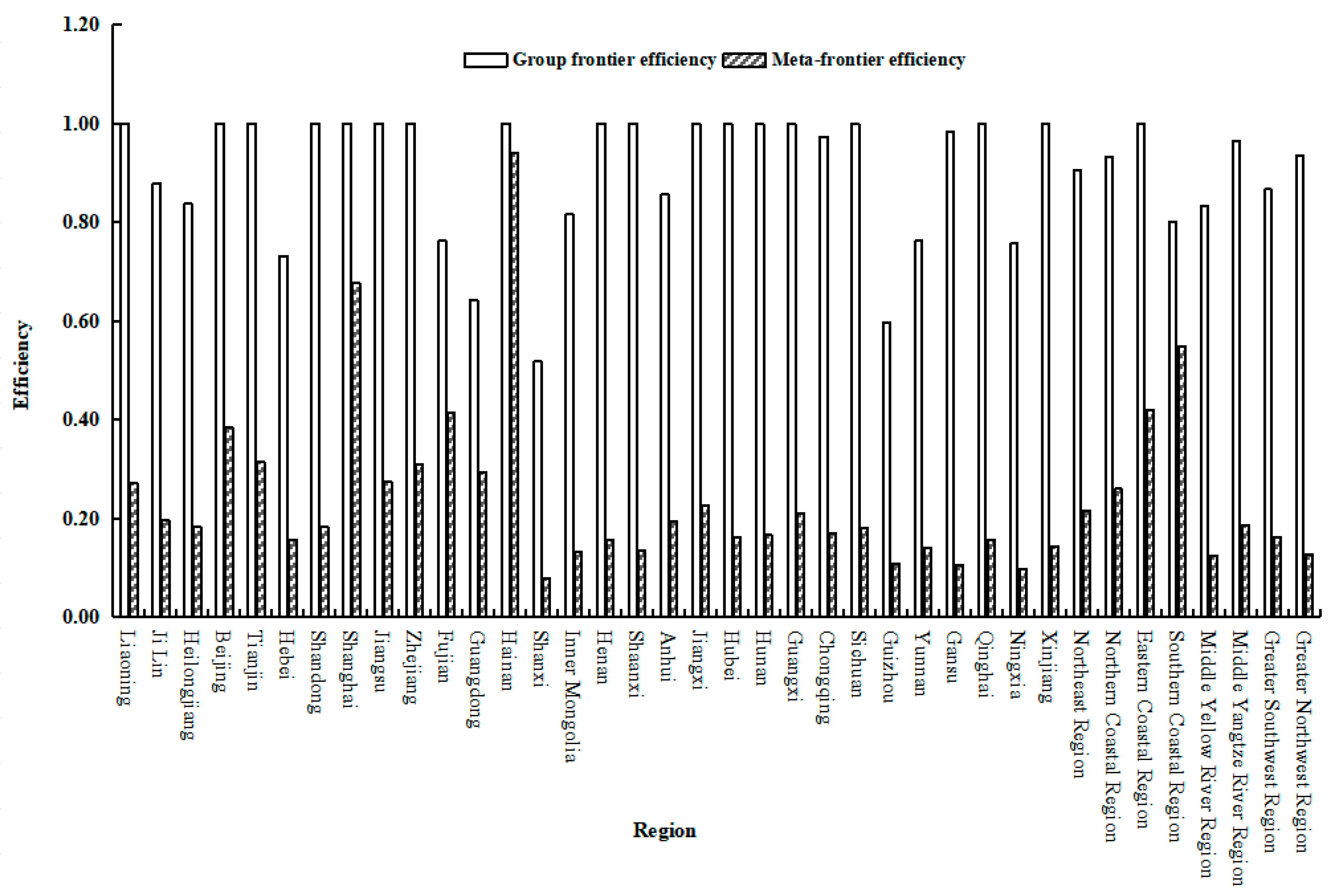
Figure 1. Average carbon emission efficiency of agriculture and rural areas in China from 2000 to 2022.
Sustainability 18 04299 g001
Figure 2. Graph showing the trend of technological gap ratio in China from 2000 to 2022.
Sustainability 18 04299 g002
Figure 3. SHAP value and feature importance under the meta-frontier.
Sustainability 18 04299 g003
Figure 4. SHAP value and feature importance under the group-frontier.
Sustainability 18 04299 g004
Figure 5. The meta-frontier feature SHAP dependence graph.
Sustainability 18 04299 g005
Figure 6. The group-frontier feature SHAP dependency graph.
Sustainability 18 04299 g006
Table 1. Descriptive statistics.
IndicatorUnitStandard DeviationMinimum ValueMaximum ValueQuantityAverage Value
Input indicatorsRural fixed asset investment108 CNY69068.24565.7550.100512.7
Employment in the primary industry104 persons690901.210680.256213569
Total sown area of crops104 hm2690534.576370.9648.8551520.940
Total power of agricultural machinery104 kW6902909.9292725.77693.97013,353
Total consumption of agricultural materials104 t690186.965144.1845.500745.160
Rural residents’ domestic energy consumption104 t of standard coal690330.355290.1124.2752009.680
Expected output indicatorsActual agricultural, forestry, animal husbandry and fishery output value108 CNY6901434.0601090.24956.9805652.878
Unexpected output indicatorsAgricultural and rural carbon emissions104 t6904095.8072603.399378.66312,029.300
Table 2. Decomposition of Inefficiency Values of Agricultural and Rural Carbon Emissions in All Chinese Provinces and Improvement Strategies.
RegionCarbon Emissions InefficiencyTechnical InefficiencyManagement InefficiencyImprovement Strategy
MeanPercentageMeanPercentageTechnologyManagement
Beijing0.6160.616100%0.0000%
Tianjin0.6840.684100%0.0000%
Hebei0.8420.57368%0.26932%
Shanxi0.9200.43848%0.48252%
Inner Mongolia0.8680.68479%0.18421%
Liaoning0.7290.729100%0.0000%
Ji Lin0.8040.68285%0.12215%
Heilongjiang0.8170.65580%0.16220%
Shanghai0.3230.323100%0.0000%
Jiangsu0.7250.725100%0.0000%
Zhejiang0.6900.690100%0.0000%
Anhui0.8050.66182%0.14418%
Fujian0.5850.34759%0.23841%
Jiangxi0.7730.773100%0.0000%
Shandong0.8160.816100%0.0000%
Henan0.8440.844100%0.0000%
Hubei0.8380.838100%0.0000%
Hunan0.8340.834100%0.0000%
Guangdong0.7070.34949%0.35751%
Guangxi0.7880.788100%0.0000%
Hainan0.0600.060100%0.0000%
Chongqing0.8300.80397%0.0263%
Sichuan0.8190.819100%0.0000%
Guizhou0.8910.48855%0.40345%
Yunnan0.8590.62172%0.23828%
Shaanxi0.8650.865100%0.0000%
Gansu0.8940.87798%0.0162%
Qinghai0.8440.844100%0.0000%
Ningxia0.9010.65873%0.24327%
Xinjiang0.8560.856100%0.0000%
National average0.7610.66587%0.09613%
Table 3. Low-carbon efficiency illusion values of agriculture and rural areas in each province of China.
Region20052010201520202022
Meta-FrontierGroup-FrontierMeta-FrontierGroup-FrontierMeta-FrontierGroup-FrontierMeta-FrontierGroup-FrontierMeta-FrontierGroup-Frontier
Beijing38.83424.612−31.5262.542−3.700−0.261−12.6626.311−35.464−11.992
Tianjin−3.285−1.6108.8300.94618.7525.17838.34834.31311.5201.257
Hebei1.000−4.4541.00094.2261.0001.31817.16539.6451.0001.000
Shanxi−1.000−1.0001.0001.0001.0001.0001.0001.0001.0001.000
Inner Mongolia1.0001.5781.000−6.3621.0001.0001.0001.0001.0001.000
Liaoning1.0000.8741.0004.5341.000−0.1041.00011.1131.000−7.667
Ji Lin1.000−5.5961.000−0.0501.0001.0001.000−2.9681.000−17.304
Heilongjiang1.0005.2471.00016.1111.000−14.5891.000−0.7201.0000.781
Shanghai−3.875−1.4126.780−0.33818.278−2.717−4.4140.06442.442−13.645
Jiangsu−24.170−1.3881.0001.2571.0000.4521.00015.7921.0003.611
Zhejiang106.329−3.17871.369−0.2761.00017.817143.7328.351−16.917−0.612
Anhui1.0005.6551.000−16.8271.0001.0001.0005.9801.000127.960
Fujian1.0001.0001.0001.0001.0001.0005.5193.1509.5943.069
Jiangxi1.0002.8361.0002.2871.0004.9411.000−2.9691.000−2.813
Shandong1.000−4.1011.0002.1991.0001.3991.0004.8231.0008.133
Henan1.000−1.3461.0000.0671.0004.5011.0001.5291.0000.565
Hubei1.0001.6411.000−4.4061.0004.4311.000−7.0061.000−4.781
Hunan1.0006.7981.0004.8091.0002.4841.000−13.4801.00030.611
Guangdong−10.629−13.3191.0001.0001.0001.0006.4210.8911.0001.000
Guangxi1.000−3.2671.0007.9161.000−4.8751.000−2.0591.000−3.445
Hainan1.2121.2111.5341.205−0.617−0.1651.1043.068−2.909−1.612
Chongqing15.332−5.6641.00013.6941.0000.7281.0001.2201.0001.942
Sichuan1.000−0.7541.000−0.7711.0000.6001.0002.5351.0002.629
Guizhou1.0001.0001.00011.8181.0001.0001.00057.9991.000−21.245
Yunnan1.0001.6571.0003.7931.0001.0001.000−1.3081.0002.880
Shaanxi1.0001.3901.0000.4251.0003.5311.000−2.3171.0006.231
Gansu1.0002.8221.0002.5311.0000.7951.000−1.3591.0001.020
Qinghai1.000−0.0991.0000.4101.0001.505−18.4308.0786.9178.754
Ningxia1.0001.0001.0001.0001.000−2.7411.0003.0251.000−5.822
Xinjiang1.000−1.1821.0000.4451.0001.0901.000−3.7261.0000.608
The number of provinces with an efficiency illusion25152923282327202719
Table 4. Selection of influencing factors.
CategoryCharacteristic VariableSymbolMeaning
Natural factorsLand disaster degreeX1Affected area/Cropland sown area
Economic factorsEconomic development levelX2Actual per capita GDP (logged)
Rural prosperity levelX3Rural residents’ per capita disposable income (logged)
Agricultural industrial structureX4(Total output value of animal husbandry + Total output value of agriculture)/Total output value of agriculture, forestry, animal husbandry and fishery
Innovation technology levelX5Domestic invention patent application acceptance volume (logged)
Social factorsRural human capital levelX6Average years of education in rural areas
Urbanization levelX7Urban population/Total population
Government factorsFiscal support for agriculture levelX8Local fiscal expenditure on agriculture, forestry and water affairs/Local fiscal general budget expenditure
Environmental regulation levelX9Investment in industrial pollution control/Industrial added value
Disclaimer/Publisher’s Note: The statements, opinions and data contained in all publications are solely those of the individual author(s) and contributor(s) and not of MDPI and/or the editor(s). MDPI and/or the editor(s) disclaim responsibility for any injury to people or property resulting from any ideas, methods, instructions or products referred to in the content.