Article

Regional Balance of Urban Multimodal Public Transport Network Based on Path Diversity

School of Mechanics and Aeronautics, Inner Mongolia University of Technology, Hohhot 010051, China
*
Author to whom correspondence should be addressed.
Sustainability 2026, 18(9), 4193; https://doi.org/10.3390/su18094193
Submission received: 29 March 2026 / Revised: 17 April 2026 / Accepted: 20 April 2026 / Published: 23 April 2026

Abstract

The imbalance of urban public transport networks often leads to traffic congestion. Traditional planning prioritizes system optimization and single-mode travel, neglecting interactions between different modes. From an economic perspective and based on passenger travel behavior, this paper constructs a reasonable path set for multimodal networks. Using information entropy, it establishes multidimensional indicators including site path diversity entropy, destination regional entropy vectors, and weighted comprehensive entropy. Regional aggregation and coefficient of variation analyze internal balance, while scatter plots and the Gini coefficient measure global resource allocation equity. ArcGIS Pro 3.4.3 is employed for spatial analysis and visualization. An empirical study of Beijing’s six central districts reveals significant spatial heterogeneity in path distribution across functional zones: working areas exhibit concentric patterns, commercial areas form corridor agglomerations, residential areas have the highest entropy values, and transport hubs are relatively balanced. Cluster analysis based on entropy vectors effectively identifies commuter, residential, and hub station types. Some hubs show an ideal “high richness, low imbalance” state, while areas like Beijing Railway Station exhibit “low richness, high imbalance.” The Gini coefficient of 0.1864 indicates relatively balanced public transport resources overall. The “route-region-demand” collaborative analysis framework constructed in this study achieves a paradigm shift from static network structure to dynamic human-oriented evaluation, providing methodological support for equity assessment, network optimization, and resource allocation in multimodal public transport networks, and can contribute to the equitable and balanced sustainable development of public transport.

1. Introduction

The fairness and equity of public resource allocation are key indicators of high-quality urban development. In particular, the regional equity of public transport network configuration directly affects the convenience of residents’ travel [1]. A well-balanced structure and layout of the public transport network can meet a greater volume of travel demand, enhance the utilization rate and network accessibility, and promote the sustainable development of multimodal public transport systems [2]. However, with the continuous advancement of urbanization, urban development models are gradually exhibiting a trend toward low density and decentralization, leading to significant spatial disparities in public transport network density and travel convenience across different regions. Traditional public transport network design typically prioritizes system optimization, which results in imbalanced layouts in some areas during the network optimization process [3]. Therefore, a reasonable evaluation of public transport network equity can improve the accessibility and utilization of the public transport system and effectively enhance the rationality of the urban travel structure [4,5]. In summary, there is an urgent need for research on the equity of public transport network layout and route distribution.
Currently, there is a substantial body of research both domestically and internationally on the structural characteristics and layout of public transport networks, with most studies focusing on network accessibility as a critical breakthrough point [6,7,8]. Quan Wei et al. utilized taxi trajectory data, employing kernel density analysis and hot spot detection methods, and introduced the coefficient of variation of regional public transport supply and demand to study bus accessibility in sensitive areas [9]. Chen Yanyan et al. adopted accessibility as a measure of service capacity for conventional public transport and validated their approach using the Beijing bus network as a case study [10]. However, most of these studies are based on a single travel mode. As public transport systems for different modes often operate independently, they lack efficient connections and coordination with one another [11,12]. Therefore, Zhao C. et al. modeled the urban multimodal transport network and measured its resilience and sensitivity [13]; Chen B. et al. integrated dynamic travel data to establish a multimodal transport network model and evaluated its disturbance resistance [14]; Liu Z. et al. constructed a multimodal transport network incorporating pedestrian data, identified critical nodes, compared changes in transport equity before and after the collapse of critical nodes using geospatial analysis, and proposed network optimization strategies [15]. Furthermore, factors such as the structure of urban travel demand, trip purposes, and temporal distribution all influence passengers’ travel choices, thereby affecting the equity of the network [15,16].
Consequently, research on the fairness and equity of public transport networks has gradually increased. Equity, a research hotspot in the socio-economic field, serves as a metric for the fairness of wealth distribution and resource allocation. Pei Yulong et al. investigated public transport network equity from the perspectives of both bus network topology and road network layout, defined its connotation, and proposed an equity measurement method combining the Gini coefficient and the Atkinson index [17]. Xu Qi et al., utilizing multiple travel modes, employed an improved two-step floating catchment area method to propose a job accessibility measurement method that considers travel costs, and evaluated the equity of regional public transport job accessibility using the Lorenz curve [18]. Based on bipartite network theory, Duan Dezhong et al. constructed a spatial dependency matrix of urban roads and bus routes, proposed spatial measure-based dependency indicators, and measured the layout impact of Beijing’s bus routes from both global and local dimensions [19]. Liu J. et al. analyzed the impact of human activities on the development of transportation systems from the perspective of human activities, approaching transportation decision-making from a human-centered perspective, aiming to provide fairer transportation planning for different population groups [20]. Concurrently, with the advancement of GIS and spatial geoinformation technologies, research integrating equity indicators with spatial visualization features has become increasingly prevalent [21]. Ben-Elia et al. started from the service coverage area of stops, using accessibility as a measure of public transport service capacity, and applied it to the study of networks such as conventional bus and bus rapid transit (BRT) [22]. Ghasemlou K. et al. proposed a user-based travel analysis method by disaggregating data on different usage patterns derived from smart card data, providing a more equitable planning foundation by accounting for users with lower trip frequencies [23]. Scholars like Cao X. et al. divided the study area into multiple traffic analysis zones (TAZs), calculated indicator values for each zone, and employed aggregate analysis to evaluate equity [24,25]. They also achieved quantitative evaluation of equity by constructing Lorenz curves and calculating the Gini coefficient area. Furthermore, the Gini coefficient, as an equity evaluation method, possesses a relatively mature theoretical foundation and classification standards and is widely used for quantifying and evaluating regional equity [26,27].
In summary, while existing research on the structure and layout of public transport networks is extensive, most findings are based on network topology and single travel modes, with limited attention given to the interactions between different travel modes and regional equity. Moreover, current research often evaluates regional equity using factors such as transit routes, surrounding economic and demographic attributes, and public transport accessibility. Few studies approach equity evaluation from the perspective of passengers’ reasonable travel paths, resulting in a lack of an evaluation system centered on travel routes. The number of reasonable travel paths available to passengers can not only reflect the transfer convenience and accessibility of a region but also indicate the supply and service capacity of its public transport. However, simply using the proportion of reasonable paths as an equity indicator cannot accurately reflect the equity of stops and regions, highlighting the need for more reasonable evaluation metrics. Based on this, building upon previous research and focusing on passengers’ actual travel characteristics, this paper establishes a method for evaluating the regional equity of multimodal public transport networks from the perspective of reasonable travel paths. It employs ArcGIS for spatial econometric analysis, aiming to provide a useful reference for the planning, design, and evaluation of urban multimodal public transport.

2. Research Framework

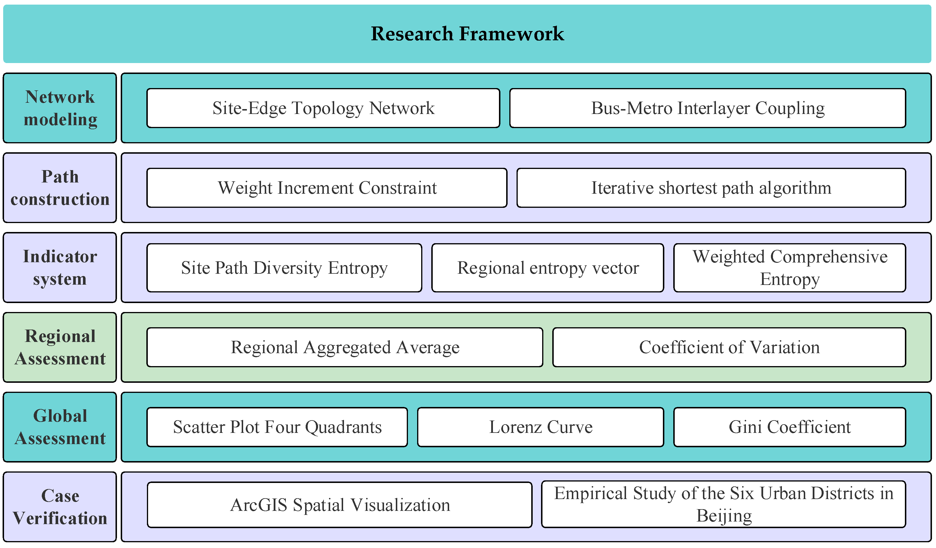
This study begins with the coupling mechanism of multimodal public transport networks, constructs a set of reasonable paths based on actual passenger travel behavior, and introduces information entropy theory to establish a multidimensional indicator system comprising stop-level path diversity entropy, destination regional entropy vectors, and weighted comprehensive entropy. By employing regional aggregation and coefficient of variation, it analyzes internal regional equity. Combined with scatter plots and the Gini coefficient, it measures the equity of global resource allocation. Using ArcGIS for spatial econometric analysis and visualization, and taking the six central districts of Beijing as a case study, it identifies the distribution characteristics of path resources and supply–demand imbalances across different functional zones. This achieves a paradigm shift from static network structure to dynamic people-oriented evaluation, providing a novel analytical framework of demand orientation–spatial equity–multimodal synergy for equity assessment and network optimization of multimodal public transport systems. The research framework is shown in Figure 1.

3. Methods for Measuring Regional Equity of Multimodal Public Transport Networks

3.1. Multimodal Public Transport Network Model

A multimodal public transport network can be abstracted as a multi-layered network consisting of nodes and edges, where nodes represent stops and edges represent routes [28]. Different layers of the network are connected through certain coupling rules. This study primarily explores regional public transport route equity based on bus and subway networks, with the coupling rules defined as follows:
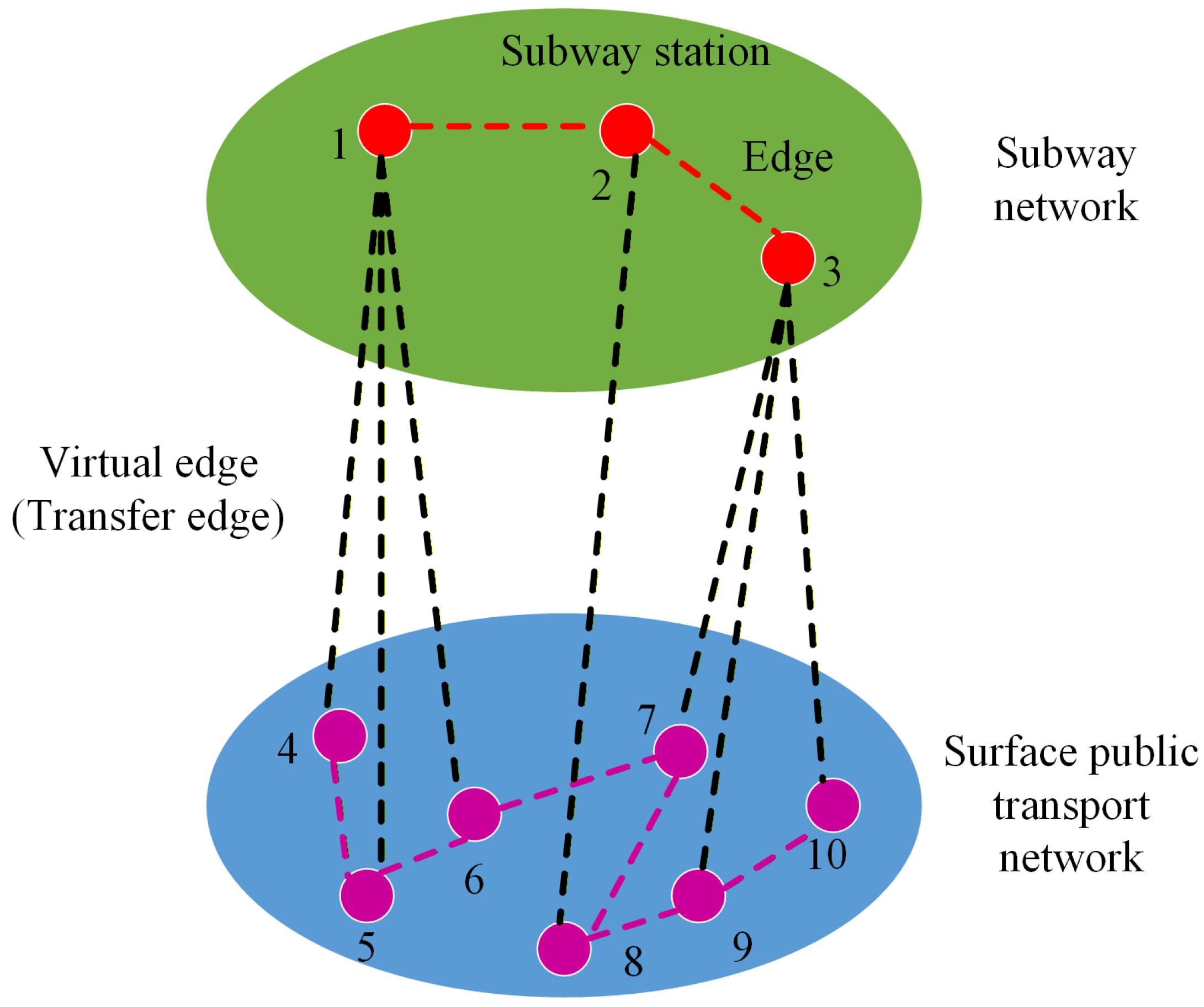
If two stops are directly connected by an edge within a single-layer network (i.e., bus or rail transit), then a r o u t e = 1 ; if two stops belong to different network layers and the rail transit stop is connected to any bus stop within a 500 m radius, then a v i r t u a l = 1 ; otherwise, no edge exists between the two stops, and the value is 0 [29]. Based on the above rules, the coupling result of the bus and subway networks is shown in Figure 2.
In the above coupling rules, bus stops within a 500 m radius of a rail transit stop are considered to be directly connected via a virtual edge, which implicitly assumes that the walking transfer process is free from physical barriers and that walking conditions are homogeneous. In real urban environments, transfer paths may be affected by factors such as building obstacles, the quality of walking facilities, and environmental safety, which can cause the actual walking distance to exceed 500 m or result in longer walking transfer times. Since this paper focuses on measuring path diversity at the topological level of multimodal public transport networks, and because the walking network within 500 m of rail transit stops in Beijing’s six central districts is generally well-developed, the actual detour distance does not greatly exceed the 500 m range. Therefore, the above idealised assumption is acceptable at the macro scale. However, when conducting refined assessments for specific hubs that face significant transfer constraints due to irreplaceable factors (e.g., Beijing Chaoyang Railway Station, which is physically blocked by railway lines), walking accessibility correction factors—such as impedance functions based on actual road network distance—can be introduced to ensure the reasonableness of stop transfer connections.

3.2. Set of Reasonable Paths and Path Diversity Index for Multimodal Public Transport Networks

3.2.1. Set of Reasonable Paths in Multimodal Public Transport Networks

During the path search process, the weight of a path consists of two components: the initial weight of the network path and the dynamic path weight of the network. The initial weight of a path in a multimodal public transport network can be expressed as the travel time of the path, as defined in Equation (1):
E w e i g h t , i = D ( s , t ) V ( s , t )
where E w e i g h t , i represents the initial travel time between two adjacent stops; D ( s , t ) represents the Euclidean distance, i.e., the straight-line distance between two adjacent stops; V ( s , t ) represents the operating speed of bus or rail transit; f denotes the adjacent stops; N is the set of stops in the multimodal public transport network.
The optimal objective for constructing a set of reasonable travel paths for passengers is to satisfy passengers’ daily detour needs while also meeting their requirements in terms of time and monetary costs. Currently, there are two main methods for calculating path sets: the K-shortest path algorithm and the completely disjoint path algorithm. Although the K paths generated by the former have relatively short weights, they often have significant overlap. Once a disruption occurs on an overlapping segment, all alternative paths sharing that segment become unusable, meaning the alternative paths lack robustness. While the path set calculated by the latter is completely non-overlapping, it imposes no constraints on path length, resulting in excessive detours and insufficient reasonableness [30]. Therefore, to suppress the repeated appearance of high-risk paths during the search process, a link weight increment function is used as a constraint. In subsequent iterations, the increased weights of higher-risk segments are gradually reduced, and the shortest path is recalculated under the new weights.
E w e i g h t , i = γ k × ( 1 β i ) δ × D s × D t L × E 0   0 < γ < 1   ,   0 < β < 1
where E w e i g h t , i represents the link weight increment between two adjacent stops; γ is the iteration parameter; β denotes the reliability of the link between adjacent stops; D is a parameter characterizing the topological properties of the multimodal public transport network node (measured by node degree in this paper); L represents the distance between adjacent stops in the multimodal public transport network; k is the iteration number; is usually relatively large, and this chapter uses the recommended value of 1.5 to 2.0 times the shortest path length [31].
Therefore, based on the above dynamic path weight calculation method, the weight of adjacent stops in this chapter can be defined as follows:
E i = E w e i g h t , i + E w e i g h t , i
In the selection of a set of reasonable paths, there are many paths between any two stops in a multimodal public transport network. However, in actual travel, only a few of these paths can meet passengers’ travel needs, while most paths are too long in distance or time-consuming. Therefore, to ensure that the reasonable paths satisfy passengers’ requirements for travel distance and time, a path constraint parameter λ is introduced to restrict the selection of reasonable paths, as shown in Equation (4):
L s , k < λ L s , 0
where L s , k represents the cost of the k -th path between any two stops in the multimodal public transport network; L s , 0 represents the cost of the shortest path; λ is a constraint parameter that can be calibrated based on passengers’ actual travel characteristics. The specific model parameters will be calibrated and introduced below.

3.2.2. Model Parameter Calibration

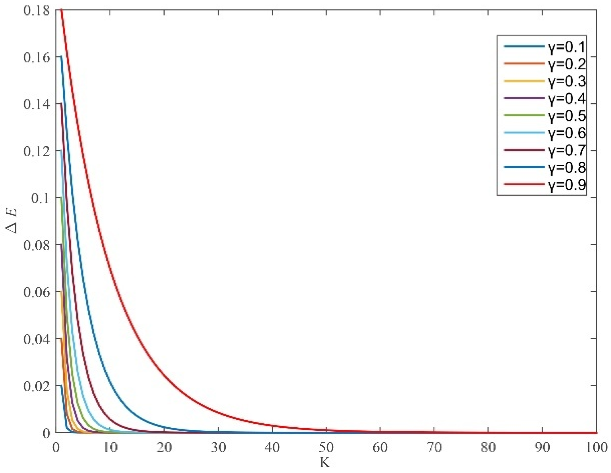
According to Equation (2), in order to prevent the link weights in the network from changing too rapidly as the number of iterations increases, the iteration parameter γ is selected for numerical simulation experiments. The value range of the iteration parameter is 0 to 1, and the specific simulation results are shown in Figure 3. It can be observed from Figure 2 that as the iteration parameter varies, the link weight increment changes continuously. Moreover, a larger iteration parameter yields results closer to the real situation. When the iteration parameter γ takes the value of 0.9, the link weight increment reaches its optimal value.
According to Equation (2), the route reliability in this chapter includes both bus route reliability and rail transit route reliability. During operation, bus networks are affected by various factors such as traffic congestion and time periods, which can cause bus route delays and thus reduce reliability. In contrast, rail transit operates in a relatively closed environment, with arrival times strictly following the train schedule, resulting in higher route reliability. Meanwhile, the virtual edges in the multimodal public transport network, which correspond to transfer edges in reality (typically realized by cycling, walking, etc.), have a reliability of 1. Therefore, in this chapter, the route reliability of the rail transit network within the multimodal public transport network is also set to 1, and the research focuses primarily on the route reliability of the bus network.
For the ground bus network, numerical simulation experiments were first conducted to verify the variation curve of ground bus route reliability with the number of iterations, as shown in Figure 4. It can be seen from Figure 4 that the higher the route reliability, the more significant the change in the link weight increment function, indicating that the route reliability parameter has an important influence on the model. Therefore, through field investigation, the reliability of ground bus routes under different time periods was statistically analyzed.
Through field investigation, 30 min periods under different time intervals (morning peak, morning off-peak, afternoon off-peak, and evening peak) were selected, and the route reliability of the ground bus network was calculated using Equation (5).
β i = T 1 m ( T f T i ) T
where β i represents the reliability of the ground bus route; T f represents the scheduled arrival time of the bus at the stop, which can be obtained from the timetable; T i represents the actual bus arrival time from field investigation; T represents the survey time; m represents the number of buses during the survey period. Therefore, based on the investigation, the route reliability of the multimodal public transport network is shown in Table 1.
According to Equation (4), in order to calibrate the reasonable path constraint parameters of the multimodal public transport network, six OD pairs in the multimodal public transport network of Beijing were selected and calibrated. The specific OD pairs are shown in Table 2.
By calculating the passenger travel time for each OD pair, the distribution of travel times across different time periods (including the 10th and 90th percentiles of travel time) was obtained. The travel time distributions for the six OD pairs are shown in Figure 5.
Based on the passenger travel time statistics for the different OD pairs mentioned above, the shortest path travel time and the average travel time for each pair were calculated. On this basis, the average value of the ratio of the average travel time to the shortest path travel time was used as the value of the constraint parameter λ for reasonable alternative paths in the model of this chapter. The specific results are shown in Table 3.
Through parameter calibration of the reasonable path selection model, the model calculates the number and direction of reasonable paths between each OD pair of stops, thereby forming a reasonable path dataset for equity evaluation.

3.2.3. Stop Path Diversity Entropy

Path diversity entropy is used to quantify the diversity and distribution uniformity of paths between network nodes. By calculating the probability distribution entropy of reasonable paths from a given stop to all other stops, the stop’s hub status and network connectivity can be evaluated. A higher entropy value indicates greater diversity in travel choices from that stop and a higher degree of hub functionality.
To calculate stop path diversity entropy, the selection of reasonable paths at a public transport stop must be transformed into probabilities before entropy calculation. This paper selects an equal-probability entropy calculation model, assuming that passengers choose randomly among all reasonable paths passing through a given public transport stop, meaning the probability of selecting any one path is equal. The formula for calculating the path diversity entropy for a single public transport stop is shown in Equation (6):
H ( s ) = i = 1 n s p i log b ( p i )
where: n s is the total number of reasonable paths originating from that stop; p i is the probability of a passenger choosing the i -th path; b is the logarithm base (the choice of logarithm base is mathematically arbitrary, but the same base must be used in all calculations within the study; different bases affect the absolute numerical values but do not affect relative ranking). In this study, the logarithm base is uniformly set to b = 1.2 , primarily for the convenience of visualization and result interpretation. This base yields entropy values distributed within the range of 0 50 , avoiding the issues of values being concentrated in a narrow band when the base is too small, or becoming too small for easy comparison when the base is too large.
The calculated value of H ( s ) can be used to evaluate the path diversity of the stop. A larger value H ( s ) indicates richer travel choices from that stop and a higher hub status. If a stop has only one reasonable path, then H ( s ) = 0 .

3.2.4. Stop Path Diversity Entropy for Destination Areas

Path diversity entropy evaluates a stop’s hub status on a global scale, so the n s in its calculation refers to the set of reasonable paths from that stop to all other stops. However, this cannot determine the relative equity of a stop within the global context. Because stop path diversity entropy is calculated using all reasonable paths from a given stop to all other stops, a stop might have many reasonable routes but, after accounting for different destinations, have fewer reasonable paths to important destination areas compared to other stops. Therefore, the path diversity from a stop to the city center versus to the suburbs has entirely different meanings, and a simple calculation of stop path diversity entropy cannot reflect the stop’s equity.
Thus, when evaluating the equity of reasonable path resources for public transport travel from different stops to various areas, judgment cannot be based solely on the number of routes passing through a stop. To address this, this paper proposes a method for calculating stop path diversity entropy based on destination areas. First, the city needs to be divided into traffic analysis zones (TAZs) and important destination areas defined, such as central business districts (CBDs), major transportation hubs, and large residential areas. Then, the OD path diversity entropy H ( s D k ) from each stop s to an important destination area D k is calculated using Equation (7):
H ( s D k ) = i P ( s , D k ) p i log b p i
where: P ( s , D k ) refers to the set of all reasonable paths from stop s to any stop within the destination area D k ; p i is the probability of a passenger choosing the i -th path; b is the logarithm base.
Based on the calculated value H ( s D k ) , different public transport stops can be evaluated for the richness of reasonable paths to the same destination, thus exploring the equity of public transport resources in terms of reasonable paths available at different origin stops while keeping the destination variable fixed.

3.2.5. Stop Entropy Feature Vector

A single entropy value often contains only simple and singular information, numerically representing a stop’s accessibility to a specific area. Therefore, this paper proposes constructing a stop entropy feature vector. Compared to a single entropy value, the entropy vector contains richer and more detailed information, more comprehensively reflecting the structural characteristics of public transport at individual stops, between stops, and across regions. The formula for the stop entropy feature vector H ( s ) is shown in Equation (8):
H ( s ) = [ H ( s D 1 ) ,   H ( s D 2 ) , ,   H ( s D k ) ]
where each component refers to the reasonable path diversity entropy from stop s to the k -th destination area.
Compared to single entropy analysis, the entropy vector can comprehensively characterize a stop’s structural pattern and facilitate cluster analysis of stops. Assuming a city has three core areas: CBD (working area), residential area (living area), and commercial center (commercial area). If stop A has an entropy vector H ( A ) = [ 3.2 ,   1.8 ,   2.5 ] , with high entropy to the working area, low entropy to the residential area, and medium entropy to the commercial area, it can be interpreted as a commute-oriented stop, primarily serving work-related travel, with average convenience for daily life services. If stop B has an entropy vector H ( B ) = [ 2.0 ,   3.1 ,   2.8 ] , it can be interpreted as a life-service-oriented stop, with poor commuting convenience.
Still using the three core areas (working, living, commercial) as an example, the entropy values from different stops to these three core areas can form entropy vectors. Cluster analysis can then be performed based on these three entropy values, as shown in Table 4, to identify different types of stops within the city.

3.2.6. Weighted Comprehensive Entropy

After establishing the entropy feature vector for a stop, compared to calculating a single comprehensive entropy, the vector allows for comprehensive entropy calculation based on different evaluation objectives. By assigning different weights to different components within the vector, the reasonable path service capabilities between stops can be compared under different research focuses or travel demands, providing data support for initial public transport route planning and operational route adjustments in response to changes in regional demand. The calculation formula is shown in Equation (9):
H w e i g h t e d ( s ) = k = 1 m w k × H ( s D k )
where: w k is the weight; H ( s D k ) is the reasonable path diversity entropy from stop s to the k -th destination area.
Regarding weight determination, when studying the equity of stops, equal weights are generally chosen for multiplying and summing the components. When studying the level of public transport service provision for travel demand, the weight for a stop’s OD entropy to each core area is typically determined by the proportion of travel groups from that stop to each core area, i.e., using OD passenger flow data. For research focusing on different travel purposes, weights can be adjusted based on the importance of regional functions. For example, if the research focuses on commuting, the weight for the working area can be increased; if the focus is on living convenience, the weights for residential and commercial areas can be increased accordingly.

3.3. Regional Path Diversity Evaluation Indicators Based on Stop Aggregation

3.3.1. Regional Path Diversity Indicators

Under different research objectives and focuses, it is necessary to calculate stop path diversity entropy, OD reasonable path diversity entropy for stop-based travel, and weighted comprehensive entropy to facilitate research on regional equity, among other aspects. When conducting research on regional travel paths, data from individual stops need to be aggregated to enable a unified study of the region. The average richness H ¯ of a region can be obtained by aver-aging the various types of path diversity entropy of stops within the study area, as shown in Equation (10):
H ¯ ( s ) = 1 M i = 1 M H ( s i )
where: M is the total number of stops in the region or traffic analysis zone (TAZ); H ( s i ) is the path diversity entropy of stop s i .
For OD-based travel, it is also necessary to calculate the average destination area path diversity entropy H ¯ ( s D k ) , which serves as a component of the coefficient of variation to evaluate the dispersion of reasonable path entropy values among stops within a region. The calculation formula is shown in Equation (11)
H ¯ ( s D k ) = 1 M i = 1 M H ( s i D k )
where: M is the total number of stops in the region or TAZ; H ( s i D k ) is the destination area (weighted) path diversity entropy of stop s i .
Representing the reasonable path diversity entropy H ( d D k ) between regions, using the averaging method of Equation (11) may obscure differences between regions. Therefore, data processing must be performed based on the selection of important destination areas. Public transport stops within the same destination area are considered components of that area. By filtering the data, the total number of reasonable paths from other public transport stops outside the destination area to all stops within that area is obtained as the total number of reasonable paths from a given stop to the destination area. Simultaneously, different origin stops are matched to traffic analysis zones. The sum of the number of reasonable paths from origin public transport stops in the same area to the destination area is considered the number of reasonable paths from the origin area to the destination area. The calculation formula is shown in Equation (12):
H ( d D k ) = i P ( d , D k ) p i log b p i
where: P ( d , D k ) refers to the set of all reasonable paths from stop d to any stop within the destination area D k ; p i is the probability of a passenger choosing the i -th path; b is the logarithm base.
Through this calculation, the average level of overall travel diversity for the traffic analysis zone can be reflected under different research focuses. A higher value indicates that passengers in the area, on average, enjoy a richer selection of paths.

3.3.2. Equity Among Stops Within a Region

When studying the diversity of travel choices within a region, average richness is used as a definition. However, in practice, focusing solely on the average reasonable path entropy value of a region can mask differences among stops within that region. It is possible that a region has a few hub stops with very high entropy values, while a large number of ordinary stops have very low values. Therefore, the differences among stops within a region cannot be ignored in the research process. In studying the disparities among stops within a region, this paper adopts indicators that reflect the dispersion of stop entropy values within the region to represent and analyze internal equity.
When studying the equity of reasonable paths among stops within a region, the coefficient of variation can intuitively reflect the dispersion of entropy values among stops. Moreover, the coefficient of variation eliminates dimensional effects, allowing direct comparison of relative inequality among regions with different average levels. The formula for the coefficient of variation C V z is shown in Equation (13):
σ z = 1 M 1 i = 1 M [ H ( s i ) H ¯ ( s ) ] 2 C V z = σ z H ¯ ( s )
where: H ( s i ) is the (destination area) path diversity entropy of stop s i ; H ¯ ( s ) is the mean value calculated from the path diversity entropy of each stop; M is the total number of stops in the region; σ z is the standard deviation of stop entropy values within the region.
Since the coefficient of variation can measure the relative disparity among stops within a region, a smaller value of the coefficient of variation C V z indicates smaller differences among stops within the region, implying that the path diversity among stops within the region is more equitable.

3.4. Methods for Measuring Regional Equity Based on Path Diversity

3.4.1. Comparison of Equity Among Stops Within Regions

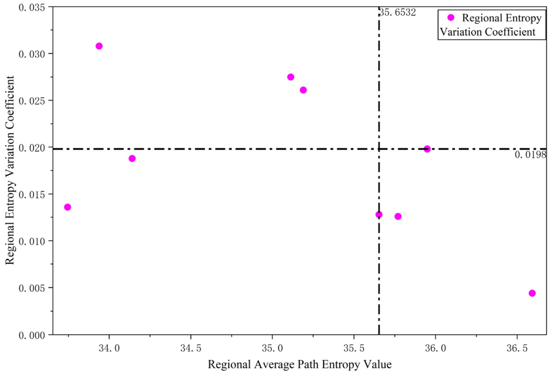
After numerically calculating the distribution equity of public transport stops within different traffic analysis zones (TAZs) or defined areas using the coefficient of variation, it is necessary to conduct a centralized comparison and evaluation of different regions from a global perspective. A scatter plot can be used for this centralized analysis. By locating the position of different regions on the scatter plot, their equity status can be evaluated from a global perspective. In the scatter plot, the average entropy value H ¯ ( s ) of each region is used as the X-axis, and the coefficient C V z of variation of entropy is used as the Y-axis. The X-axis represents the average richness of reasonable paths in the region, while the Y-axis represents the equity among stops within different regions.
When establishing the coordinate axes, it is first necessary to calculate the median of the average path entropy values for all regions and the median of the coefficients of variation of entropy for all regions. Then, the quadrants of the scatter plot are established using these two medians as the axes. Finally, the data for each region are plotted on the scatter plot. The position of each region on the scatter plot represents its level of richness and equity on a global scale.
To objectively evaluate the relative position of each transport hub area within the global context, the scatter plot is divided into four quadrants using the median of the average entropy values of all areas as the X-axis dividing line, and the median of the coefficients of variation of all areas as the Y-axis dividing line. The median, rather than the mean, is chosen as the cut-off point because it is insensitive to extreme values and thus more robustly reflects the central tendency of the dataset. Moreover, using the median ensures that the numbers of samples in the high and low groups are approximately equal, avoiding group imbalance caused by skewed distributions.
The median of the average path entropy values serves as the dividing line for the X-axis. Regions with values greater than the median are located on the right side, indicating higher richness; regions with values less than the median are located on the left side, indicating lower richness. The median of the coefficients of variation of entropy serves as the dividing line for the Y-axis. Regions with values greater than the median are located above, indicating high imbalance; regions with values less than the median are located below, indicating low imbalance. As shown in Table 5, the four quadrants have the following interpretations within the global context.
Through the scatter plot and quadrant division, the relative level of equity in stop distribution within regions at the overall urban level can be evaluated more objectively.

3.4.2. Evaluation of Global Urban Public Transport Resource Distribution Equity

This paper uses the Gini coefficient based on the set of stop reasonable path diversity indices to test the regional equity of multimodal public transport. The specific formula is shown in Equation (14) [32].
f ( ) = S 1 S 1 + S 2 S 2 = 0 1 f ( )   d ( ) S 1 = 1 2 S 2
where: is a formal parameter, referring to the path diversity entropy of stops in this paper; f ( ) is the Gini coefficient for indicator ; S 1 is the area enclosed by the Lorenz curve and the line of absolute equality; S 2 is the area enclosed by the Lorenz curve and the line of absolute equality.
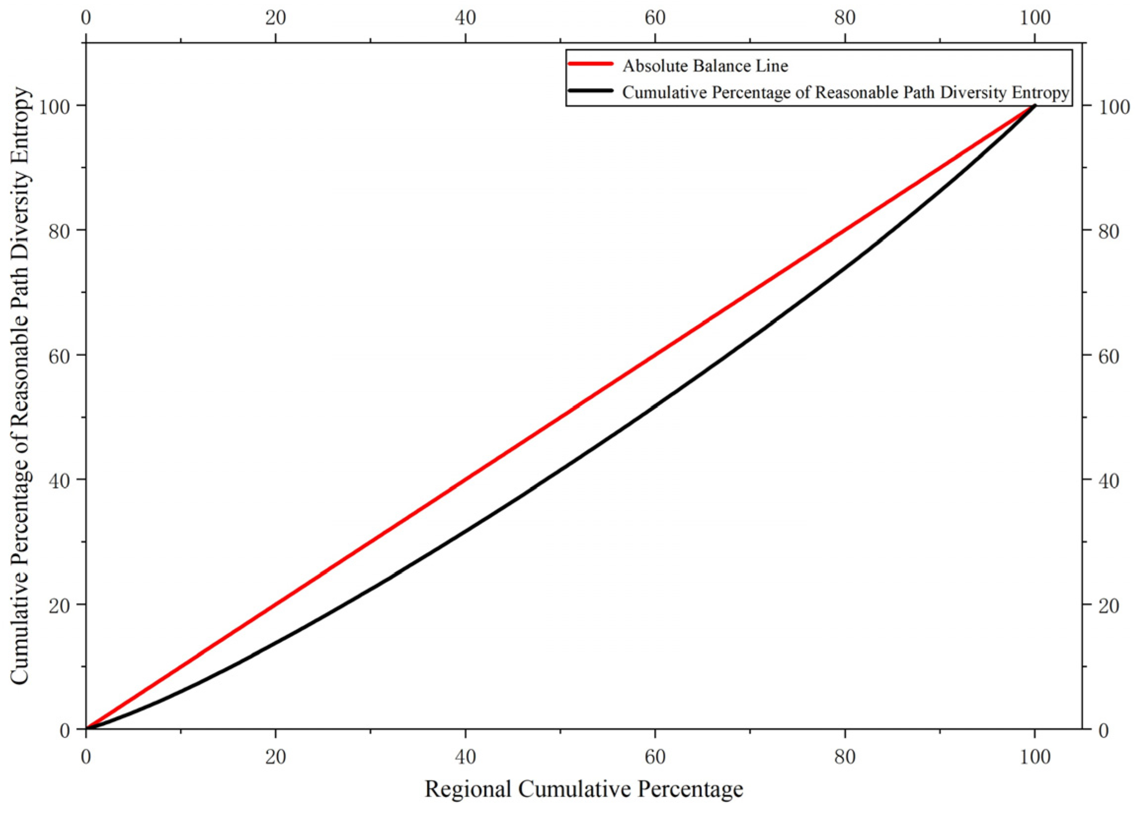
When plotting the Lorenz curve, the obtained path diversity entropy values of each stop or region are first sorted from smallest to largest. The cumulative proportion of stops or regions is then used as the X-axis, for example, the first 10% of stops (regions), the first 20% of stops (regions), and so on. The cumulative proportion of path diversity entropy is used as the Y-axis, representing the cumulative proportion of the total path diversity index held by these stops or regions. Finally, the Lorenz curve is plotted using the resulting dataset. In the figure, the more curved the Lorenz curve (i.e., the more it deviates from the line of absolute equality, the diagonal), the more unequal the distribution of public transport resources in the city as a whole [33].
f ( ) characterizes the gap between the current distribution of the research object and the ideal situation of absolute equality. It is a quantitative representation of the area between the Lorenz curve and the line of absolute equality. A larger value indicates a more unequal distribution of current urban public transport resources. The international evaluation standards for the Gini coefficient are shown in Table 6.

4. Case Study

This paper takes the public transport network of Beijing as the research object. By obtaining information on Beijing’s public transport network, data cleaning and correction are performed using TransBigData 0.5.3. A topological model of the public transport network is established, and various diversity indicators are analyzed. ArcGIS Pro 3.4.3 is used for spatial visualization analysis and presentation. Specifically, this paper takes the six central districts of Beijing (Dongcheng, Xicheng, Chaoyang, Haidian, Fengtai, and Shijingshan) and the Beijing Capital International Airport area as the case study objects. Using the spatial clipping and division functions of ArcGIS Pro, the six central districts of Beijing are extracted and divided into 359 traffic analysis zones (TAZs). Within these six central districts, there are a total of 3251 public transport stops. Topological connections between public transport stops and topological connections between stops across different layers of the public transport network within a reasonable range have been established. The division of TAZs in the six central districts of Beijing is shown in Figure 6.

4.1. Case Analysis of Stop and Regional Path Diversity Indices

4.1.1. Diversity Entropy of Total Reasonable Paths for Public Transport Stops and Regions

Using the public transport stop and connection information, the reasonable paths from each stop to other stops were calculated using Equation (2). A dataset of reasonable paths for stop-based travel was established, obtaining the number of reasonable paths from each stop to every other stop, as well as the total number of reasonable paths passing through each stop. The total number of reasonable paths passing through each stop allows for a macroscopic assessment of the richness of reasonable paths for each stop and region. Assuming passengers choose routes randomly with equal probability, the path diversity entropy for a single public transport stop was calculated using Equation (6). In this paper, a logarithm base of 1.2 is used for calculating stop path diversity entropy. A scatter plot was created with the total number of reasonable paths passing through public transport stops on the X-axis and the entropy values on the Y-axis. The scatter plot of the diversity entropy of total reasonable paths per stop is shown in Figure 7.
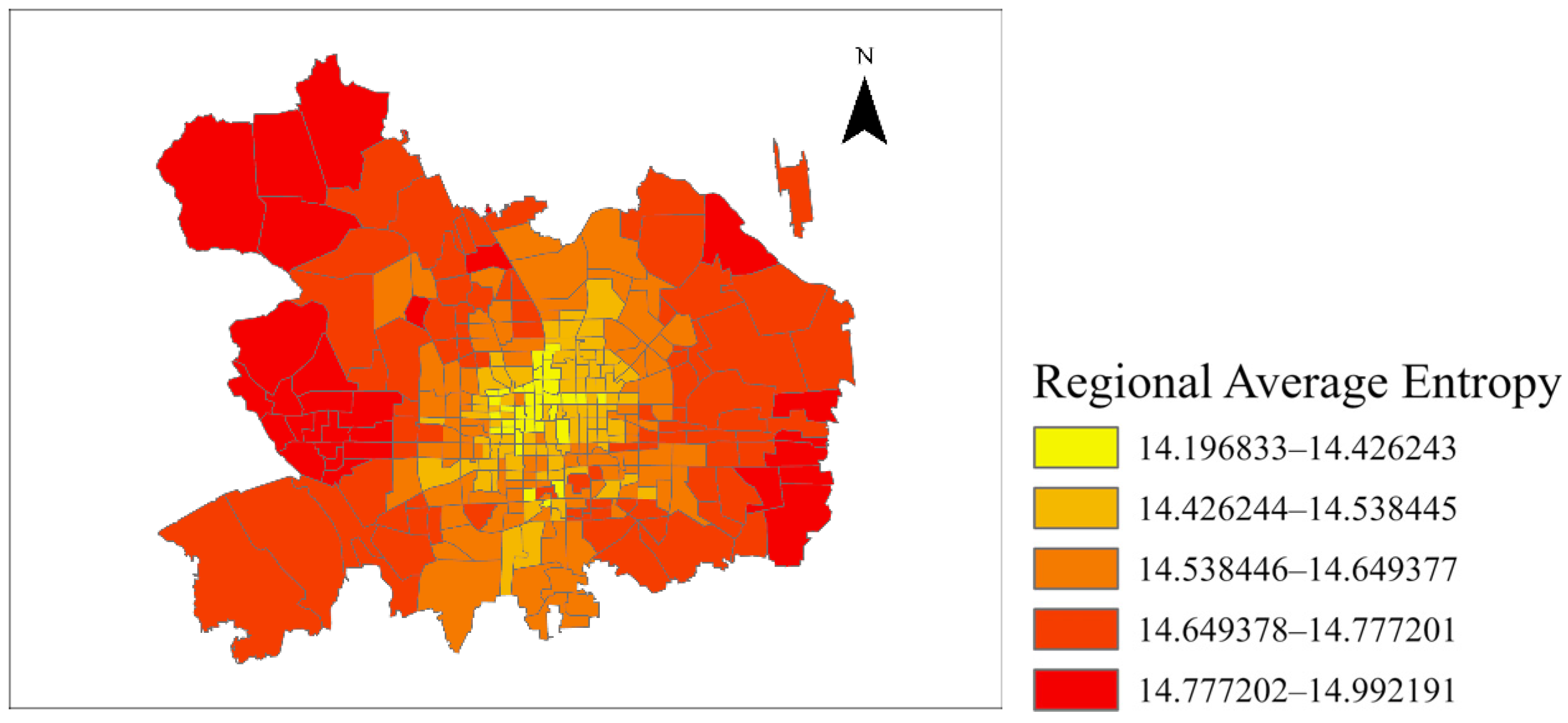
As shown in the figure, among the 3251 public transport stops within the six central districts of Beijing, after analyzing the total number of reasonable paths passing through each stop and calculating the diversity entropy, it can be observed that in terms of richness, the diversity of public transport travel across stops in Beijing’s six central districts shows little variation, and route concentration is generally good. Subsequently, based on the stop path diversity entropy, the regional public transport travel diversity entropy for TAZs was calculated using Equation (10), yielding the regional richness of the public transport network. Visualization of regional richness was performed using ArcGIS Pro. The distribution map of the diversity entropy of total reasonable paths for TAZs in the six central districts is shown in Figure 8.
The color depth in the figure reflects the magnitude of path diversity entropy for each TAZ. Darker colors indicate higher average path diversity for the region as a travel origin. In terms of spatial distribution, entropy values are generally higher in the central urban area, such as parts of Dongcheng, Xicheng, Chaoyang, and Haidian, indicating that when these areas serve as origins, passengers have access to a richer set of reasonable paths and stronger network connectivity. In contrast, entropy values are relatively lower in Fengtai, Shijingshan, and peripheral parts of the six central districts, suggesting that travel path choices from these origins are relatively limited, possibly due to insufficient network coverage or inconvenient transfers. Adding bus routes or optimizing transfer nodes in low-entropy areas could enhance the diversity and convenience of regional travel.

4.1.2. Selection of TAZs for Key Destination Areas and Reasonable Path Diversity Entropy for Destination Areas

Within the scope of Beijing’s six central districts, this case study selects TAZs for four key destinations: working areas (CBDs), commercial areas, major residential areas, and transport hub areas. Based on relevant literature and established facts, the boundaries of these different key areas are defined, thereby determining their locations within the divided TAZs of the six central districts and the number of public transport stops within them.
For the selection of a working area in Beijing’s six central districts, the Zhongguancun industrial park areas are chosen as the case study working area. Liu Xiaobing et al. [34] identified the central layout of 35 metropolitan areas in China using Baidu map data, finding that Beijing exhibits a typical unbalanced polycentric urban structure, with nearly half of its employment located within the Fifth Ring Road. Employment centers are mainly distributed in areas such as the Pan-CBD, Zhongguancun, Financial Street, Wangjing, and Fengtai Science Park [35]. This paper selects the employment concentration area of Zhongguancun Science Park as the working area for research. Zhongguancun Science Park, a concentration of high-tech industries in China, houses nearly 30,000 high-tech enterprises and a large working population. The park is bounded by Suzhou Street to the west, the Beijing-Baotou Railway to the east, North Third Ring Road West to the south, and Chengfu Road to the north, covering an area of approximately 5.91 km2. The land use is primarily commercial and high-tech industrial zones, generating significant work-related public transport travel demand. In the TAZ division, Zhongguancun Science Park corresponds to areas 446, 449, 450, and 451, containing a total of 28 public transport stops.
For the selection of a commercial area in Beijing’s six central districts, the Beijing CBD is chosen as the case study commercial area. The Beijing CBD is an emerging urban commercial center [36]. The study area is bounded by Dongdaqiao Road to the west, Xidawang Road to the east, Tonghuihe North Road to the south, and Chaoyang North Road to the north, with a core area of approximately 3.99 km2. Land use is primarily commercial and financial districts, characterized by high pedestrian traffic and significant commercial travel demand. The core area of the Beijing CBD corresponds to TAZ 252, containing 10 public transport stops.
For the selection of major residential areas in Beijing’s six central districts, representative suburban concentrated residential areas with a jobs–housing separation pattern are chosen as the case study residential areas. Meng Bin et al. [37,38,39,40] analyzed commuting times and jobs–housing balance across several different residential areas in Beijing. Their selection of representative residential areas included Changping Residential Area, Wangjing Residential Area, Huilongguan Residential Area, and Fangzhuang Residential Area. This paper combines these four concentrated residential areas into one overall representative area for research. The corresponding TAZ numbers and the number of public transport stops within them are shown in Table 7.
For the selection of transport hub areas in Beijing’s six central districts, several dispersed multimodal transport areas are chosen as the case study transport hub areas. Multiple comprehensive multimodal transport hubs are distributed within Beijing’s six central districts, including Beijing Railway Station, Beijing North Railway Station, Beijing South Railway Station, Beijing West Railway Station, Beijing Fengtai Railway Station, Beijing Chaoyang Railway Station, Qinghe Railway Station, Liuliqiao Long-Distance Bus Hub, and the Beijing Capital International Airport area. This paper combines these nine key hub areas into one overall transport hub area for research. The corresponding TAZ numbers and the number of public transport stops within them are shown in Table 8.

4.1.3. Reasonable Path Diversity Entropy for Destination Areas

Based on the TAZ division, the defined destination areas (e.g., working area) for the case study are set as the trip endpoints. The public transport stops within these areas serve as the specific destinations. Using the dataset of reasonable paths between origins and destinations, the data are matched. Areas outside the destination area are considered origin areas. By counting the number of reasonable paths from public transport stops in other areas to public transport stops in the destination area, and using the number of reasonable paths between areas, the regional reasonable path diversity entropy from other areas to the specified destination area can be calculated using Equation (12). Based on the regional reasonable path entropy values obtained for different important destinations, the entropy values for each origin area are visualized using ArcGIS Pro.
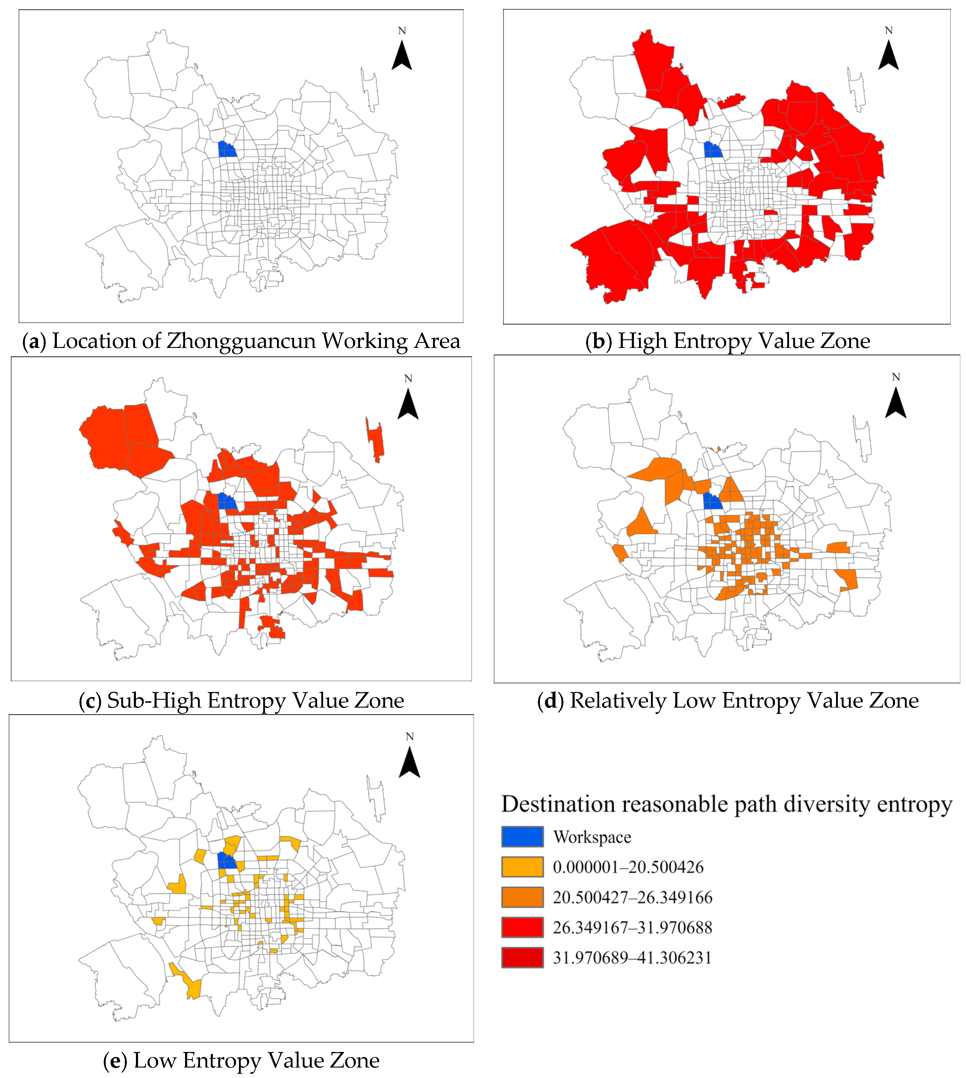
Following the selection of the working area, areas 446, 449, 450, and 451 are set as the destination areas. The number of reasonable paths from stops in other areas to these areas is counted, and entropy values are calculated using Equation (12). The distribution map of reasonable path diversity entropy for other areas with the working area as the destination is shown in Figure 9.
The blue area in the northwest of the central districts in Figure 6 is the selected Zhongguancun working area, an important destination area. The distribution of reasonable travel paths across areas generally exhibits a concentric pattern, with high values in the core and lower values on the periphery. Focusing on the key destination area, it can be observed that entropy values in areas surrounding Zhongguancun are significantly higher than in outer suburban areas, indicating that commuting path resources are highly concentrated in the employment core. Furthermore, it can be seen that the reasonable path entropy values from major residential areas on the urban periphery to the working area are relatively high. This distribution pattern aligns with the urban jobs–housing spatial structure and can meet the efficient travel needs of a large commuting population.
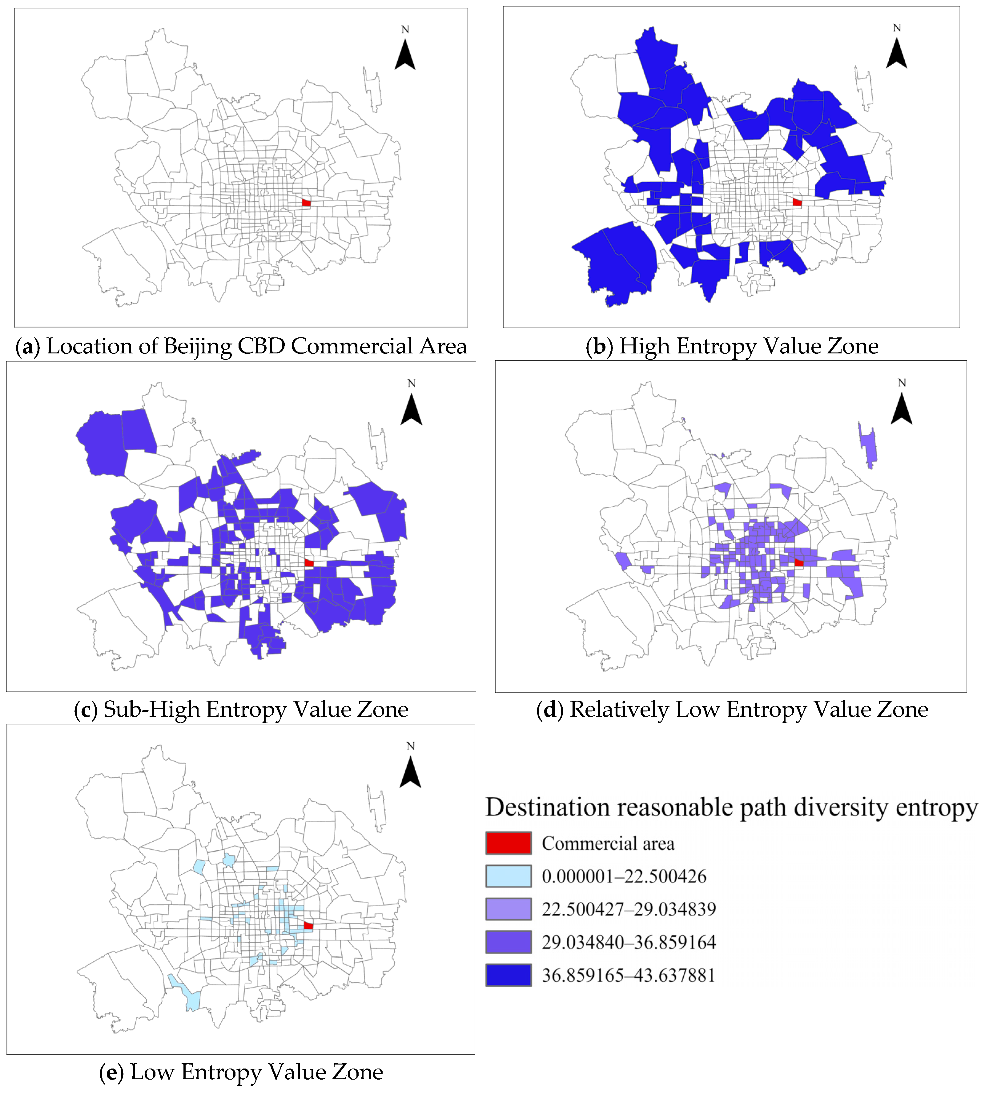
Following the selection of the commercial area, area 252 is set as the destination area. The number of reasonable paths from stops in other areas to this area is counted, and entropy values are calculated using Equation (12). The distribution map of reasonable path diversity entropy for other areas with the commercial area as the destination is shown in Figure 10.
The red area in the eastern part of the central districts in Figure 7 is the selected Beijing CBD commercial area, an important destination area. The distribution of reasonable travel paths across areas exhibits an irregular spatial pattern. High-entropy areas form corridor-like agglomerations radiating from the CBD towards the northwest, northeast, and southwest, while there is a noticeable break in high entropy towards the southeast. Some areas immediately adjacent to the core even show medium-to-low entropy values. The urban periphery is not uniformly low in entropy; instead, there are multiple patches of high or sub-high entropy formed around transport hubs and main bus routes. Low-entropy areas are scattered in patches or isolated clusters in the southwestern outskirts and northeastern margins. As a commercial core area, the path diversity to the commercial area is not determined by linear distance from the CBD but is instead dominated by the layout of the bus network and the direction of main corridors. The radiation capacity varies significantly across different directions, with network orientation playing a much greater role than distance orientation, ensuring convenience for shopping, office, and other trips.
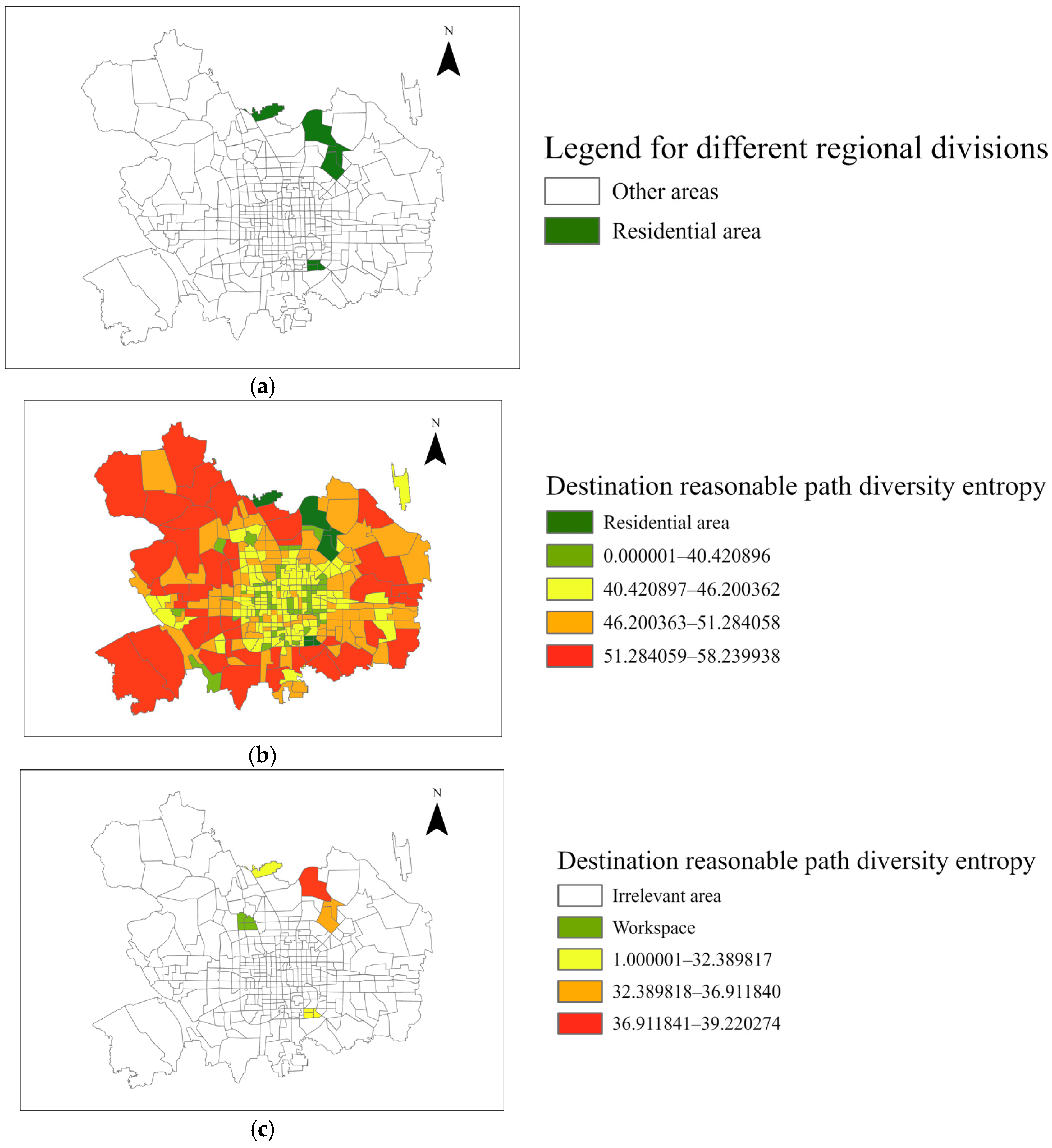
Following the selection of residential areas, the areas listed in Table 4 are set as the destination areas. The number of reasonable paths from stops in other areas to these areas is counted, and entropy values are calculated using Equation (12). The distribution map of reasonable path diversity entropy for other areas with the residential areas as the destination is shown in Figure 11.
The collection of green areas in the northern and southeastern parts of the central districts in Figure 8 represents the four major residential areas selected as important destination areas. It can be observed that when these four major residential areas are the destinations, the maximum entropy value is 58.24, which is significantly higher than that for the working and commercial areas. This is because residential areas are high-density population zones with higher supporting bus network densities and more comprehensive stop coverage. The high-entropy distribution highly overlaps with the residential areas themselves, adequately meeting residents’ diverse daily travel needs. Additionally, analyzing the reasonable path diversity entropy for the jobs–housing commuting type between each residential area and the Zhongguancun working area reveals that the entropy values for the four residential areas show little difference. This confirms that, within the peripheral residential areas of Beijing’s six central districts, the richness of reasonable paths for commuting to work is relatively high, capable of meeting the diverse commuting needs of the working population living in these areas.
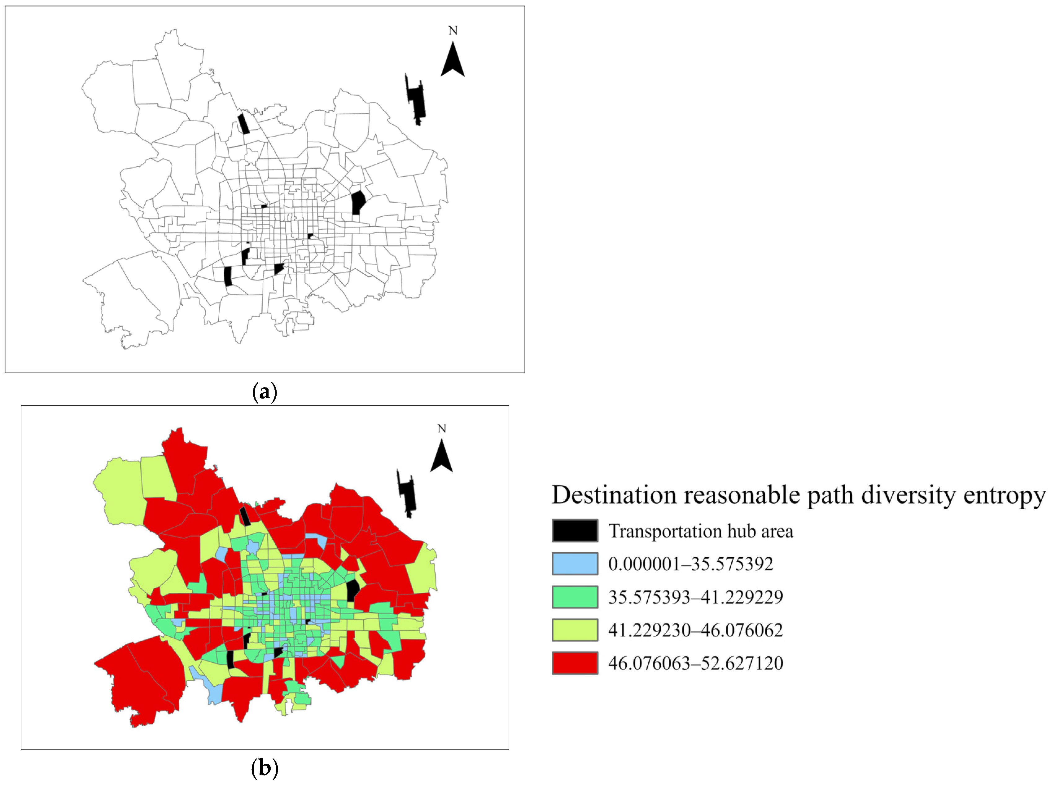
Following the selection of transport hub areas, the areas listed in Table 5 are set as the destination areas. The number of reasonable paths from stops in other areas to these areas is counted, and entropy values are calculated using Equation (12). The distribution map of reasonable path diversity entropy for other areas with the transport hub areas as the destination is shown in Figure 12.
The collection of black areas surrounding the central districts and including the Beijing Capital International Airport area in Figure 9 represents the nine transport hub areas selected as important destination areas. The maximum entropy value is 52.63, falling between that of residential areas and that of commercial/working areas. The entropy distribution is relatively balanced, with no obvious extreme high-value areas. This is attributed to the dispersed layout of the transport hubs and the fact that they are all multimodal transfer nodes. This distribution characteristic ensures travel convenience for people from different urban areas to reach the hubs, supporting efficient connections between external and internal urban transport.

4.1.4. Comparative Evaluation of Stop Entropy Feature Vectors

Using Equation (7), the destination entropy from each public transport stop to specific destination areas can be calculated. According to Equation (8), entropy vectors can be established using multiple destination area entropy components. Comparing the entropy vectors of multiple stops allows for the identification of differences between stops, forming a table of relative functional type classifications for stops, similar to Table 1.
Based on the division of Beijing’s six central districts and the selection of important destination areas, this study uses stops in the residential area with the largest residential population and highest travel demand as an example. Taking the Changping Central Residential Area as an example, five public transport stops within TAZ 557 are randomly selected. Based on the number of reasonable routes from these stops to the working area, commercial area, and transport hub areas, each entropy component for each stop is calculated using Equation (7), yielding the entropy vector for each stop and an evaluation. The stop IDs, entropy vectors, and relative type evaluations for these five stops are shown in Table 9.

4.1.5. Comparative Evaluation of Weighted Comprehensive Entropy

For research on weighted comprehensive entropy, different research focuses typically determine the weights of entropy components, or weights are determined based on passenger flow data, and calculations are performed using Equation (9). This allows for an objective comparison of the travel matching capabilities of different stops under the same demand within a unified weighted entropy system.
Taking the five stops in Table 6 as an example, a higher weight is assigned to the travel demand for the working area, while the remaining weight is equally divided between the commercial area and transport hub areas. Thus, the final weight for the working area is set to 0.6, and the weights for the commercial area and transport hub areas are both set to 0.2. The weighted comprehensive entropy for each stop is calculated using Equation (9), and the results are shown in Table 10.
By simulating the weights based on travel demand, the weighted comprehensive entropy calculation reveals that when the travel distribution ratio to the working area, commercial area, and transport hub areas is 6:2:2, Stop 4463 best matches the passenger flow demand oriented towards the working area.

4.2. Regional Equity Evaluation Based on Path Diversity

4.2.1. Comparison of Equity Among Stops Within Regions

Travel from stops can also vary significantly among different stops within a region. Using a scatter plot can intuitively reflect the relative positions of different stops within the overall stop set, providing an objective relative evaluation of equity among stops.
Taking the major transport hub areas in Beijing as an example, and considering the distribution of the main migrant worker residential population in Beijing, this study takes the Changping Central Residential Area selected in this paper as the destination. It explores the reasonable paths from each public transport stop in various transport hub areas to the Changping Central Residential Area, as well as the relative disparity in reasonable path entropy values among public transport stops within each transport hub area. The relative disparity among different transport hub areas is compared using the distribution of points on a scatter plot of regional average entropy vs. coefficient of variation.
Using the set of reasonable paths between pairs of public transport stops, the number of reasonable paths from any stop in a transport hub area to any stop in the Changping Central Residential Area can be obtained. Consequently, the number of reasonable paths from any stop in the transport hub area to the Changping Central Residential Area can be determined. The coefficient of variation C V z for each transport hub area is then calculated using Equation (13). The scatter plot of regional average entropy vs. coefficient of variation is shown in Figure 13.
Based on the internal coefficient of variation of stops in each area and their positions in the figure, the following observations can be made:
First Quadrant: Characterized by high average entropy and high coefficient of variation, including areas like “Beijing Fengtai Railway Station.” This indicates that the overall path richness in this area is high, but internal differences among stops are significant. There may be a few hub stops concentrating a large amount of path resources.
Second Quadrant: Characterized by low average entropy and high coefficient of variation, including areas like “Beijing Railway Station,” “Beijing Chaoyang Railway Station,” and “Beijing Capital International Airport.” This indicates that overall path choices in these areas are limited, and internal resource distribution is uneven, with some stops having very few paths.
Third Quadrant: Characterized by low average entropy and low coefficient of variation, including areas like “Beijing North Railway Station” and “Beijing South Railway Station.” Overall path resources in these areas are scarce, but differences among stops are small, indicating generally weak service capacity.
Fourth Quadrant: Characterized by high average entropy and low coefficient of variation, including areas like “Beijing West Railway Station,” “Qinghe Railway Station,” and “Liuliqiao Long-Distance Bus Hub.” This represents an ideal state, where the area has rich path resources and even distribution, allowing passengers diverse and equitable travel choices.
The specific positions and types of each area in the figure are shown in Table 11.
For Beijing Railway Station, Beijing Chaoyang Railway Station, and the Beijing Capital International Airport area, which are located in the second quadrant of Figure 13, a further analysis of the causes of their poor performance is provided below:
Beijing Railway Station, as a traditional railway hub built in 1959, has its surrounding bus stop layout constrained by the spatial limitations of the historic urban area. Stop spacing is uneven, and the transfer distance to Metro Line 2 is long, resulting in a relatively low number of effective alternative paths in the set of reasonable paths. Moreover, the passenger flow at Beijing Railway Station is mainly composed of low-frequency long-distance travelers on conventional trains and suburban rail passengers, as well as tourists, who have a relatively weak demand for path diversity in the urban multimodal public transport network. Furthermore, historical planning did not reserve sufficient transfer space, causing path resources to become concentrated in a few stops.
Beijing Chaoyang Railway Station is a newly built high-speed railway station, but the supporting bus and rail transit services in its surrounding area lagged behind the station’s opening. The number of public transport resources serving the station is limited. In addition, physical barriers caused by railway lines and expressways force walking transfer distances between bus stops and station entrances to exceed reasonable thresholds, requiring detours from some directions. This directly restricts the number of reasonable paths with this station as an origin or destination, leading to significant differences in path diversity among stops within the area.
The Beijing Capital International Airport area, as a special functional zone, relies mainly on airport express trains and airport buses, with low coverage of conventional ground buses. Most stops are located on the periphery of the terminals. Due to the physical boundaries of the airport security check zone and terminals, connectivity between stops within the airport area is weak. Moreover, passengers are highly time-sensitive, have a low demand for path diversity, and focus more on travel efficiency. These factors objectively result in a situation of “limited overall path choices and significant internal differences” in this area.
In summary, the “low richness, high imbalance” state of these hubs is not accidental but the result of the interplay of historical planning legacies, physical spatial constraints, and passenger demand characteristics. For these areas, simply increasing the total number of routes is not the optimal solution; instead, spatially targeted transfer improvements should be implemented. For areas with spatial constraints due to historical planning, such as Beijing Railway Station, priority should be given to optimizing pedestrian direct-access corridors and local micro-circulation connecting the station with surrounding public transport stops. For areas where newly built facilities lag behind, such as Beijing Chaoyang Railway Station, the opening of radial feeder routes and high-capacity, multi-direction rail transit lines should be accelerated to fully integrate the station into the urban public transport network. For areas with functional particularities, such as Capital Airport, shuttle buses between internal stops should be strengthened, and public transport routes connecting to other multi-direction hub stations should be introduced. On this basis, feeder connections between conventional buses and rail transit should be increased, and walking and transfer conditions around stops should be improved.

4.2.2. Evaluation of Global Urban Public Transport Resource Distribution Equity Under Different Travel Demands

By plotting and analyzing the Gini coefficient and Lorenz curve, the equity of overall urban resource distribution can be evaluated. Furthermore, for specific travel demands, such as traveling to a fixed destination like a working area or commercial area, a targeted global equity analysis can be conducted. The analysis can also be performed with stops or regions as independent units. Using stops as independent units yields more detailed results, better capturing changes in equity. Using regions as independent units yields more macroscopic results, providing a preliminary analysis from a macro perspective and offering suggestions for micro-level adjustments.
This paper selects the working area as the destination, uses the calculation from Equation (14), and plots the Lorenz curve to present the Gini coefficient equity analysis with regions as independent units. The Lorenz curve is shown in Figure 14.
The calculation based on Equation (14), comparing the Lorenz curve with the line of absolute equality obtained using regions as independent units, yields a Gini coefficient value of 0.1864. According to the international Gini coefficient evaluation standards, when conducting global equity analysis with regions as independent units, from a macro perspective of TAZs, the distribution of public transport resources in Beijing’s six central districts is in a state of absolute equity. As the central area of Beijing, the disparity in public transport resources among the various TAZs is not significant, and the public’s travel needs are generally met.
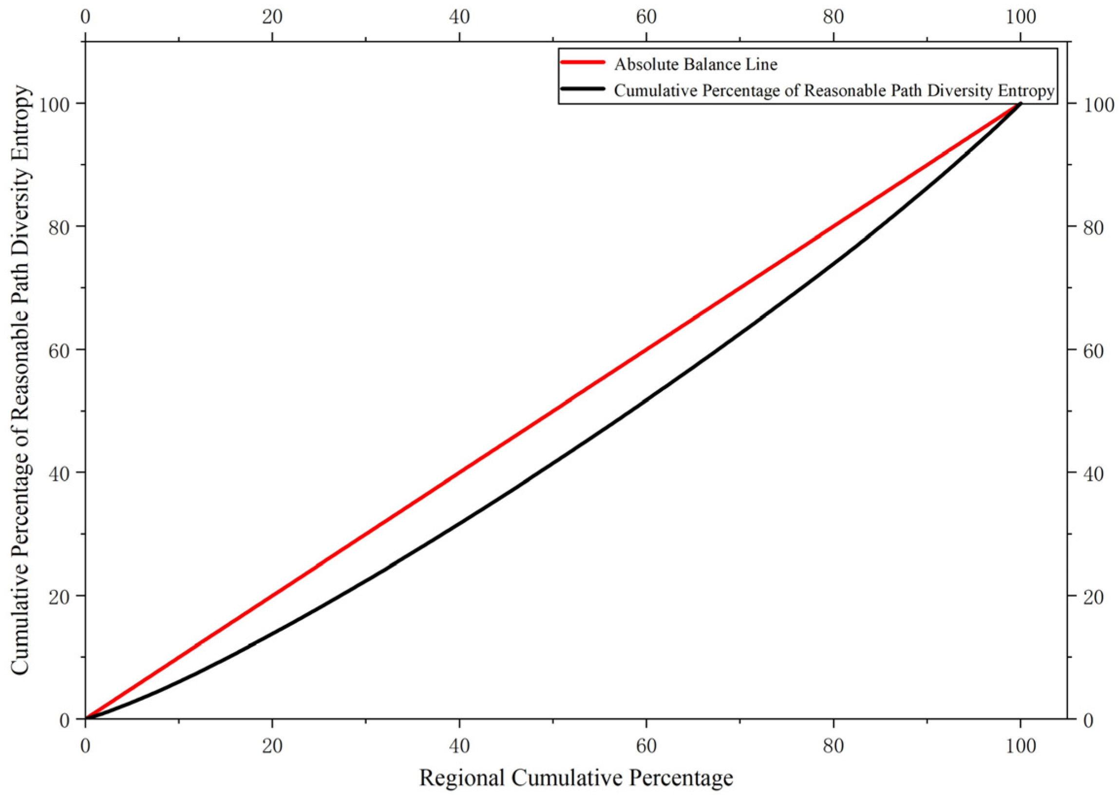
Meanwhile, taking the working area as the destination, a Gini coefficient equity analysis with individual public transport stops as independent variables is provided, and the Lorenz curve is shown in Figure 15.
According to Equation (10), the Lorenz curve obtained with regions as independent variables is compared with the line of absolute equality, yielding a Gini coefficient of 0.0565. According to the international Gini coefficient evaluation standards, this value also falls within the range of absolute equity and is even lower than the Gini coefficient at the regional level. This result indicates that when stops are taken as the independent units, the distribution of public transport resources is more equitable than at the regional level. The reason is that regional aggregation averages out high-entropy and low-entropy stops within the same area, thereby amplifying apparent differences between regions. In contrast, the stop-level analysis directly reflects the path diversity of each individual stop. Due to the high density of stops and adequate network coverage in Beijing’s six central districts, the entropy values of the vast majority of stops are concentrated at the medium-to-high level, resulting in a lower Gini coefficient. Both scales support the conclusion of “absolute equity,” demonstrating the robustness of our findings across different aggregation scales. It should be noted, however, that macro-level global equity, even when absolute, does not imply the absence of low-entropy areas or stops. In practical planning, targeted optimization of low-entropy areas or stops is necessary. It is also recommended that both scales be consulted in actual planning: the regional scale for macro-level resource allocation, and the stop scale for identifying specific low-entropy stops for precise optimization.


5. Discussion and Planning Recommendations

5.1. Main Conclusions

Starting from the path diversity of multimodal public transport networks, this paper achieves a quantitative measurement and visual representation of regional equity in public transport networks through multidimensional indicators such as stop path diversity entropy, destination regional entropy vectors, and weighted comprehensive entropy, combined with spatial econometric analysis methods. An empirical study is conducted using the six central districts of Beijing as a case study.
The research findings indicate that path diversity entropy values in Beijing’s central urban area are generally higher than those in peripheral areas, and the distribution of paths across different functional zones exhibits significant spatial heterogeneity, with distinct characteristics in working areas, commercial areas, residential areas, and transport hubs. Stop function classification based on entropy vectors effectively identifies stop types such as commuter-oriented, life-oriented, and hub-oriented stops. Weighted comprehensive entropy can reflect the service matching capability under different travel demands. Internal equity varies across regions, with some transport hubs exhibiting an ideal state of “high richness, low imbalance,” while other areas suffer from “low richness, high imbalance.” The global Gini coefficient is 0.1864, indicating that the overall distribution of public transport resources among TAZs is relatively equitable. However, significant differences in path diversity still exist among stops within individual regions. For example, some transport hub areas such as Beijing Railway Station and Beijing Chaoyang Railway Station exhibit the characteristics of “low richness, high imbalance,” while other areas such as Beijing West Railway Station and Qinghe Railway Station achieve the ideal state of “high richness, low imbalance.” This coexistence of macro-level overall equity with micro-level internal inequity within some regions suggests that aggregate fairness does not necessarily guarantee service equity within each individual area, and there remains considerable room for refining local resource allocation.
The “route–region–demand” collaborative analysis framework constructed in this study achieves a shift from static network structure to dynamic people-oriented evaluation, providing methodological support for equity assessment, network optimization, and resource allocation in multimodal public transport networks. The analytical framework constructed in this paper can identify spatially mismatched areas of public transport resources and stop-level path diversity differences, thereby helping to enhance the social equity of network layout and facilitating research on network resilience. By reducing passengers’ inefficient detours and optimizing resource allocation, the framework also has positive implications for environmental emission reduction and operational economic efficiency. Therefore, the research findings can make a positive contribution to steering multimodal public transport networks toward greater sustainability. However, the transfer radius assumption in the network coupling rules of this paper does not account for the influence of factors such as building obstacles in the actual walking environment. In future research, data such as walking networks can be integrated to construct a coupling model based on actual walking impedance. Furthermore, this paper does not yet incorporate real-time passenger flow data or travel preferences, and the model’s dynamic responsiveness needs improvement. Future research could introduce multi-source data for validation and extend the analysis to more cities for comparative studies to enhance the generalizability and practical applicability of the conclusions.

5.2. Recommendations for Urban Transport Planning and Management

Based on the above research findings, the following specific recommendations are proposed for optimizing the equity of multimodal public transport networks in Beijing and similar high-density megacities:

5.2.1. Differentiated Network Optimization Strategies by Zone

For areas with high richness but high imbalance (e.g., Beijing Fengtai Railway Station area), the total number of routes should not be blindly increased in public transport network planning. Instead, the connections between stops within the area should be optimized. By linking low-entropy stops with hub stops, the accessibility of low-entropy stops can be improved, preventing excessive concentration of resources on a few hubs. For areas with low richness and high imbalance (e.g., Beijing Railway Station, Beijing Chaoyang Railway Station, and Capital Airport area), feeder routes between conventional buses and rail transit should be increased, walking and transfer conditions around stops should be improved, and short-distance circulator buses or shared mobility services should be prioritized at low-entropy stops. For areas with low richness and low imbalance (e.g., Beijing North Railway Station and Beijing South Railway Station areas), the overall network density should be comprehensively increased, with a focus on adding outward radial routes to enhance external accessibility and avoid a “low-level equilibrium”.

5.2.2. Functional-Zone-Oriented Allocation of Public Transport Resources

For working areas (e.g., Zhongguancun area), the “concentric” high-entropy coverage should be maintained and strengthened. During peak hours, directional express services or express trains on rail transit serving major residential areas should be introduced to reduce the number of transfers for commuting and improve travel efficiency for cross-regional jobs–housing commuters. For commercial areas (e.g., Beijing CBD area), given the “corridor agglomeration” pattern, radial trunk lines and perpendicular feeder routes should be strengthened to prevent commercial accessibility from relying excessively on a few transport corridors. For large residential areas (e.g., Huilongguan, Wangjing, etc.), the advantage of high entropy values should be preserved, with emphasis on ensuring the diversity of jobs–housing commuting paths and direct connectivity during peak hours, thereby avoiding systemic risks caused by single-path dependence.

5.2.3. Dynamic Resource Allocation Mechanism Under Different Travel Demands

The data-supporting role of weighted comprehensive entropy in resource allocation should be leveraged to dynamically identify areas that are currently disadvantaged in terms of commuting, commercial, or living orientation. When travel demand patterns change, the weight coefficients of destination areas and resource allocation plans should be adjusted in advance, achieving a proactive demand-oriented response for resource allocation updates.

Author Contributions

Conceptualization, J.T. and J.J.; methodology, J.T. and J.J.; software, J.T. and J.J.; validation, J.T.; formal analysis, J.T.; investigation, J.J.; resources, J.J.; data curation, J.T.; writing—original draft preparation, J.T.; writing—review and editing, J.J.; visualization, J.T.; supervision, J.J.; funding acquisition, J.T. and J.J. All authors have read and agreed to the published version of the manuscript.

Funding

This research was funded by the National Natural Science Foundation of China (No. 52462046), Natural Science Foundation of Inner Mongolia Autonomous Region (No. 2024QN05046), Innovation and Entrepreneurship Training Program for Chinese College Students (No. 202510128010); Inner Mongolia University of Technology Professional and Innovation Integration Course Development Project (No. ZC2024012).

Institutional Review Board Statement

Not applicable.

Informed Consent Statement

Not applicable.

Data Availability Statement

The data presented in this study are available upon approved request from the corresponding author, due to institutional ethical research and data management processes.

Conflicts of Interest

The authors declare no conflicts of interest.

Abbreviations

The following abbreviations are used in this manuscript:
CBDCentral Business District
TAZTraffic Analysis Zone
ODOrigin–Destination
BRTBus Rapid Transit
GISGeographic Information System

References

  1. Editorial Department of China Journal of Highway and Transport. Review on China’s Traffic Engineering Research Progress: 2016. China J. Highw. Transp. 2016, 29, 1–161. [Google Scholar]
  2. Welch, T.F.; Mishra, S. A Measure of Equity for Public Transit Connectivity. J. Transp. Geogr. 2013, 33, 29–41. [Google Scholar] [CrossRef]
  3. Tao, T.; Cao, J. Exploring nonlinear and collective influences of regional and local built environment characteristics on travel distances by mode. J. Transp. Geogr. 2023, 109, 103599. [Google Scholar] [CrossRef]
  4. Chen, Z.; Haynes, K.E. Multilevel assessment of public transportation infrastructure: A spatial econometric computable general equilibrium approach. Ann. Reg. Sci. 2015, 54, 663–685. [Google Scholar] [CrossRef]
  5. Manitz, J.; Harbering, J.; Schmidt, M.; Kneib, T.; Schöbel, A. Source estimation for propagation processes on complex networks with an application to delays in public transportation systems. J. R. Stat. Soc. 2017, 66, 521–536. [Google Scholar] [CrossRef]
  6. Sun, Z.; Zacharias, J. Transport equity as relative accessibility in a megacity: Beijing. Transp. Policy 2020, 92, 8–19. [Google Scholar] [CrossRef]
  7. Li, L.; Ren, H.; Zhao, S.; Duan, Z.; Zhang, Y.; Zhang, A. Two dimensional accessibility analysis of metro stations in Xi’an, China. Transp. Res. Part A Policy Pract. 2017, 106, 414–426. [Google Scholar] [CrossRef]
  8. Chen, Z.S.; Wang, Y.; Chen, Y.H.; Mardani, A.; Pedrycz, W.; Martínez, L. Towards a collective opinion generation approach with multiple objectives for evaluating rail transit station accessibility in urban areas. Knowl.-Based Syst. 2024, 294, 111721. [Google Scholar] [CrossRef]
  9. Sun, C.; Quan, W. Evaluation of Bus Accessibility Based on Hotspot Detection and Matter-Element Analysis. IEEE Access 2020, 8, 138800–138809. [Google Scholar] [CrossRef]
  10. Chen, Y.Y.; Wei, P.Y.; Lai, J.H.; Feng, G.H.; Li, X.; Gong, Y. A Calculation Method of Area Public Transit Accessibility Based on GIS. J. Transp. Syst. Eng. Inf. Technol. 2015, 137, 132–140. [Google Scholar]
  11. Wang, Y.; Li, J.; Shu, X. A Review and Perspectives on Complex Network Theory and Its Application in Transportation System Resilience. In Proceedings of the 28th International Symposium on Advancement of Construction Management and Real Estate; Lecture Notes in Operations Research; Springer Nature: Singapore, 2024; pp. 677–690. [Google Scholar]
  12. Zhang, L.; Wen, H.; Lu, J.; Li, S.; Lei, D. Vulnerability assessment and visualization of large-scale bus transit network under route service disruption. Transp. Res. Part D Transp. Environ. 2020, 88, 102570. [Google Scholar] [CrossRef]
  13. Zhao, C.; Fei, M.A.; Cui, R.; Ren, W. Metropolitan area multimodal transportation network modeling and integrated resilience measurement. J. Tsinghua Univ. Sci. Technol. 2025, 65, 1930–1944. [Google Scholar]
  14. Chen, B.; Wang, B.; Pan, S.; Wu, J.; He, Z. On the Resilience Evaluation of Urban Multimodal Transportation Network Considering Dynamic Travel Demand. Transp. Res. Rec. 2026, 2680, 519–549. [Google Scholar] [CrossRef]
  15. Liu, Z.; Dong, K.; Xu, Y.; Lin, D.; Deng, M. Urban multimodal network resilience: Graph-geospatial analysis of post-collapse impact and transit equity in Baltimore. GeoJournal 2025, 90, 185. [Google Scholar] [CrossRef]
  16. Orlando, V.M.; Degano, I.L.; Lotito, P.A. Social optimum in public transport networks when users choose strategies: Analysis and comparison with Wardrop equilibrium. Ann. Oper. Res. 2025, 349, 1785–1815. [Google Scholar] [CrossRef]
  17. Almutairi, A.; Owais, M.; Ahmed, A.S. Notes on bus user assignment problem using section network representation method. Appl. Sci. 2024, 14, 3406. [Google Scholar] [CrossRef]
  18. Pei, Y.; Jin, Y.; Chang, Z. Equilibrium of Topology and Layout of Urban Multimode Public Transit Network. China J. Highw. Transp. 2021, 34, 127–138. [Google Scholar]
  19. Xu, Q.; Chen, Y.; Huang, J.; Gao, S.; Zhang, Z. Job Accessibility Analysis Considering Travel Cost. J. Transp. Syst. Eng. Inf. Technol. 2022, 22, 37–44. [Google Scholar]
  20. Liu, J.; Yang, X.; Luo, L.; Li, J.; Chen, H.; An, R.; Li, J. Inspecting urban transit-oriented development from the perspective of human activity: A case study of Xi’an, China. J. Transp. Geogr. 2025, 128, 104381. [Google Scholar] [CrossRef]
  21. Duan, D.; Liu, C.; Du, D.; Gui, Q. Spatial dependency of bus-line distribution based on bipartite network: A case study of Beijing city. Acta Geogr. Sin. 2016, 71, 2185–2198. [Google Scholar]
  22. Zhang, L.; Lu, J.; Fu, B.; Li, S.B. A Review and Prospect for the Complexity and Resilience of Urban Public Transit Network Based on Complex Network Theory. Complexity 2018, 2018, 2156309. [Google Scholar] [CrossRef]
  23. Ben-Elia, E.; Benenson, I. A Spatially-explicit Method for Analyzing the Equity of Transit Commuters’ Accessibility. Transp. Res. Part A Policy Pract. 2019, 120, 31–42. [Google Scholar] [CrossRef]
  24. Ghasemlou, K.; Ergun, M.; Dadashzadeh, N. Exploring equity in public transportation planning using smart card data. Sensors 2021, 21, 3039. [Google Scholar] [CrossRef]
  25. Cao, X.; Chen, H.; Liang, F.; Wang, W. Measurement and Spatial Differentiation Characteristics of Transit Equity: A Case Study of Guangzhou, China. Sustainability 2018, 10, 1069. [Google Scholar] [CrossRef]
  26. Fang, J.Y. Evaluation of Urban Public Transportation Network Equilibrium Based on Gini Coefficient. J. Transp. Syst. Eng. Inf. Technol. 2012, 12, 178–183. [Google Scholar]
  27. Lucas, K.; Van Wee, B.; Maat, K. A method to evaluate equitable accessibility: Combining ethical theories and accessibility-based approaches. Transportation 2016, 43, 473–490. [Google Scholar] [CrossRef]
  28. Song, Y.; Kim, H.; Lee, K.; Ahn, K. Subway Network Expansion and Transit Equity: A Case Study of Gwangju Metropolitan Area, South Korea. Transp. Policy 2018, 72, 148–158. [Google Scholar] [CrossRef]
  29. Schakenbos, R.; La Paix, L.; Nijenstein, S.; Geurs, K.T. Valuation of a transfer in a multimodal public transport trip. Transp. Policy 2016, 46, 72–81. [Google Scholar] [CrossRef]
  30. Wang, Z.; Song, J.; Zhang, Y.; Li, S.; Jia, J.; Song, C. Spatial Heterogeneity Analysis for Influencing Factors of Outbound Ridership of Subway Stations Considering the Optimal Scale Range of “7D” Built Environments. Sustainability 2022, 14, 16314. [Google Scholar] [CrossRef]
  31. Jia, J.L.; Huang, Y.W.; Zhang, W.T.; Chen, Y.Y.; Liu, Z. A Route Diversity-Based Approach for Estimating Vulnerability of Stations in a Multimodal Public Transport Network. J. Adv. Transp. 2024, 2024, 6995651. [Google Scholar] [CrossRef]
  32. Chen, Y.Y.; Wang, D.Z. Heuristic algorithm for emergency candidate paths with high reliability. J. Beijing Univ. Technol. 2010, 36, 1242–1247. [Google Scholar]
  33. Artekin, A.O.; Kalayci, S. Comparative analysis of Gini coefficient, GDP, energy consumption, and transportation modes on CO2 using NARDL (Nonlinear Distributed Lag Autoregressive Model) for the USA. Sustainability 2024, 16, 9030. [Google Scholar] [CrossRef]
  34. Delbosc, A.; Currie, G. Using Lorenz curves to assess public transport equity. J. Transp. Geogr. 2011, 19, 1252–1259. [Google Scholar] [CrossRef]
  35. Liu, X.B.; Li, F.X.; Tian, X.M.; Yan, X.D. Identifying Metropolitan Center Structure Based on Commuting Patterns. J. Transp. Syst. Eng. Inf. Technol. 2022, 22, 17–28. [Google Scholar]
  36. Han, H.; Yang, C. Spatial Pattern Evolution of Residential and Industrial Land and Its Impact on Commuting Behavior in Beijing Metropolitan Area. Econ. Geogr. 2019, 39, 65–75. [Google Scholar]
  37. Long, Y.; Zhang, Y.; Cui, C. Identifying commuting pattern of Beijing using bus smart card data. Acta Geogr. Sin. 2012, 67, 14. [Google Scholar]
  38. Bin, M.; Yu, H.L.; Zheng, L.M. The Analysis of Commuting Behavior in the Huge Residential Districts: A Case Study of Wangjing and Tiantongyuan in Beijing. Geogr. Res. 2012, 31, 2069–2079. [Google Scholar]
  39. Meng, B. The spatial organization of the separation between jobs and residential locations in Beijing. Acta Geogr. Sin. 2009, 64, 1457–1466. [Google Scholar]
  40. Zhan, D.; Meng, B. Spatial clustering analysis of residential and employment distribution in Beijing based on their social characteristics. Acta Geogr. Sin. 2013, 68, 1607–1618. [Google Scholar]
Figure 1. Research Framework.
Sustainability 18 04193 g001
Figure 2. Schematic Diagram of Multimodal Public Transport Network Coupling.
Sustainability 18 04193 g002
Figure 3. The iterative inhibitor γ vary with the number of iterations.
Sustainability 18 04193 g003
Figure 4. The reliability varies with the number of iterations.
Sustainability 18 04193 g004
Figure 5. Distribution of travel times between OD pairs. (a) The travel time distribution of Jintailu Station to Guomao station; (b) The travel time distribution of Liuliqiao Station to Beijing South Railway station; (c) The travel time distribution of Zhichunlu Station to Guomao station; (d) The travel time distribution of Zhichunlu Station to Beijing West Railway station; (e) The travel time distribution of Zhichunlu Station to Guomao station; (f) The travel time distribution of Xidan Station to Guomao station.
Sustainability 18 04193 g005
Figure 6. Schematic diagram of TAZ division in the six central districts of Beijing.
Sustainability 18 04193 g006
Figure 7. Scatter plot of the diversity entropy of total reasonable paths per stop.
Sustainability 18 04193 g007
Figure 8. Distribution map of the diversity entropy of total reasonable paths for TAZs in the six central districts.
Sustainability 18 04193 g008
Figure 9. Composite distribution map of reasonable path diversity entropy for other areas with the working area as the destination.
Sustainability 18 04193 g009
Figure 10. Composite distribution map of reasonable path diversity entropy for other areas with the commercial area as the destination.
Sustainability 18 04193 g010
Figure 11. Composite distribution map of reasonable path diversity entropy for other areas with the residential areas as the destination. (a) Location of Major Residential Areas; (b) Distribution Map of Reasonable Path Diversity Entropy for Other Areas with Residential Areas as the Destination; (c) Distribution Map of Reasonable Path Diversity Entropy from Each Residential Area to the Working Area.
Sustainability 18 04193 g011
Figure 12. Composite distribution map of reasonable path diversity entropy for other areas with the transport hub areas as the destination. (a) Location of Transport Hub Areas; (b) Distribution Map of Reasonable Path Diversity Entropy for Other Areas with Transport Hub Areas as the Destination.
Sustainability 18 04193 g012
Figure 13. Scatter plot of regional average entropy vs. coefficient of variation for each transport hub area with the Changping Central Residential Area as the destination.
Sustainability 18 04193 g013
Figure 14. Lorenz curve with regions as independent units.
Sustainability 18 04193 g014
Figure 15. Lorenz curve with stops as independent variables.
Sustainability 18 04193 g015
Table 1. The calibration results of reliability parameter.
Time PeriodMetro Line ReliabilityVirtual Line ReliabilityBus Line ReliabilityTime Period
Morning Peak110.65Morning Peak
Morning Off-Peak110.80Morning Off-Peak
Afternoon Off-Peak110.85Afternoon Off-Peak
Table 2. The distribution of OD pairs for case study.
CaseOriginDestinationSample Count
1Jintailu StationGuomao Station80
2Liuliqiao StationBeijing South Railway Station61
3Zhichunlu StationGuomao Station134
4Zhichunlu StationBeijing West Railway Station45
5Liuliqiao StationGuomao Station134
6Xidan StationGuomao Station262
Table 3. The calibration results of constraint parameter.
OD PairOriginDestinationShortest Path Time (min)Average Travel Time (min)Constraint Parameter
1Jintailu StationGuomao Station1015.651.57
2Liuliqiao StationBeijing South Railway Station2736.161.34
3Zhichunlu StationGuomao Station3641.141.14
4Zhichunlu StationBeijing West Railway Station2333.791.47
5Liuliqiao StationGuomao Station3747.731.29
6Xidan StationGuomao Station1620.881.30
Table 4. Main types of urban public transport stops based on entropy vectors using three core areas as an example.
Cluster CategoryTypical Entropy Vector PatternRepresentative Stop
Versatile Hub[High, High, High]Large downtown transfer station
Commute-Oriented Stop[High, Low, Medium]Suburb-to-city commuter stop
Life-Oriented Stop[Low, High, Medium]Large residential area stop
Shopping-Oriented Stop[Medium, Medium, High]Stop near commercial district
Isolated Stop[Low, Low, Low]End-of-line stop
Table 5. Interpretation of quadrants in the scatter plot comparing equity of stop distribution within regions.
QuadrantCharacteristicDescription
First QuadrantHigh richness, high imbalanceThe region offers many travel choices overall, but there are significant internal differences. Typically, this is an urban core area.
Second QuadrantLow richness, high imbalanceThe least desirable type. The region offers few travel choices overall, and resources are highly concentrated in a few stops.
Third QuadrantLow richness, low imbalanceTravel choices are relatively scarce overall. Commonly found in newly developed areas or low-density peripheral areas.
Fourth QuadrantHigh richness, low imbalanceThe target state for network planning and optimization. The region not only offers abundant travel choices overall but also distributes convenience relatively evenly among stops.
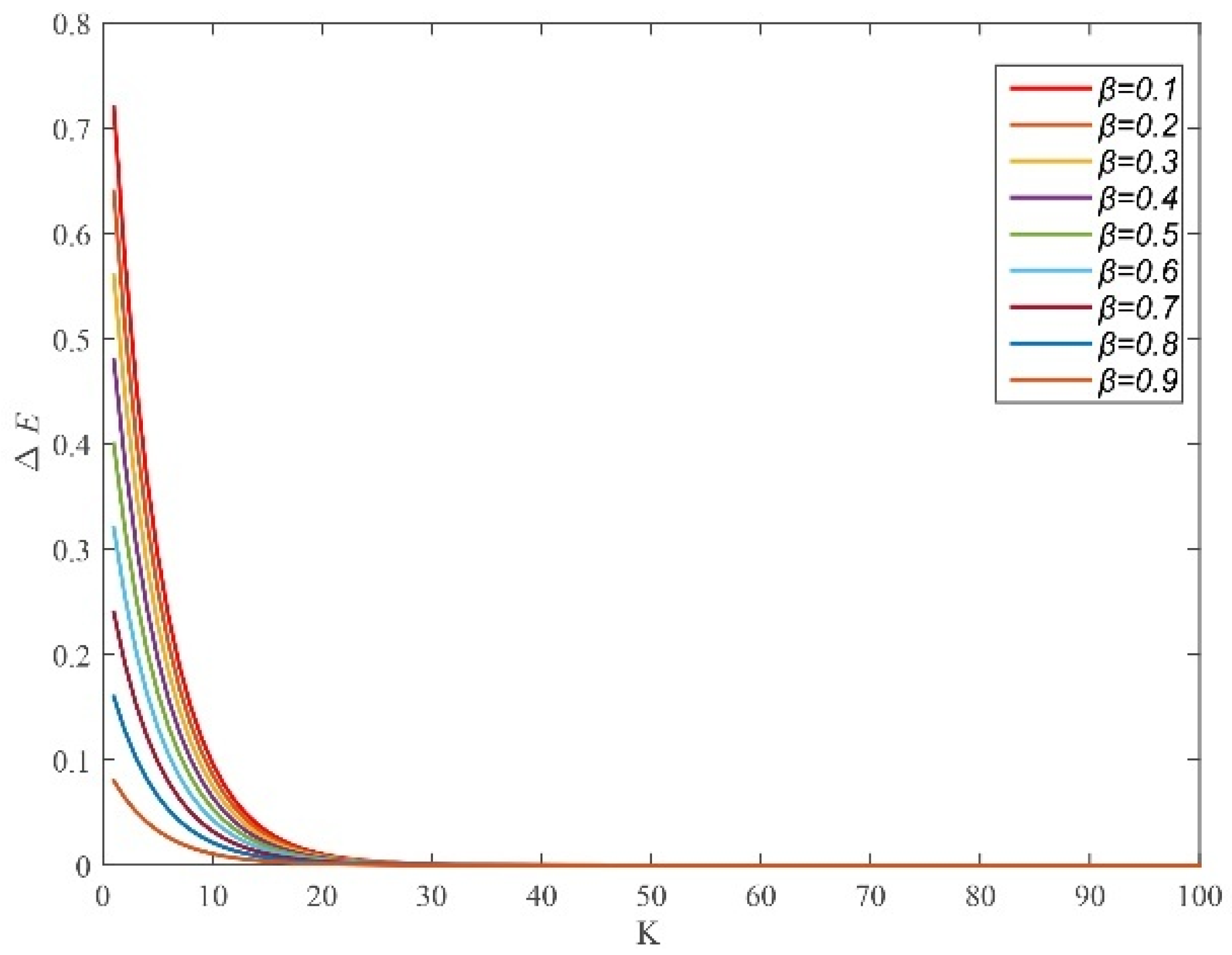
Table 6. International evaluation standards for the Gini coefficient.
f ( ) [0, 0.2)[0.2, 0.3)[0.3, 0.4)[0.4, 0.5)[0.5, 1]
RatingAbsolutely equalRelatively equalModerately equalUnequalHighly unequal
Table 7. Correspondence information of representative residential areas in TAZ division.
Representative Residential Area NameTAZ Number(s)Number of Internal Public Transport Stops
Changping Central Residential Area55761
Wangjing Residential Area272, 27574
Huilongguan Residential Area147, 54920
Fangzhuang Residential Area420, 421, 42222
Table 8. Correspondence information of different transport hubs in TAZ division.
Transport Hub NameTAZ Number(s)Number of Internal Public Transport Stops
Beijing Railway Station3925
Beijing North Railway Station4622
Beijing South Railway Station4304
Beijing West Railway Station4762
Beijing Fengtai Railway Station49717
Beijing Chaoyang Railway Station28516
Qinghe Railway Station52214
Liuliqiao Long-Distance Bus Hub4908
Beijing Capital International Airport Area5594
Table 9. Entropy vectors and type evaluations for five random stops in the Changping Central Residential Area.
Stop IDStop NameEntropy VectorEntropy Vector CharacteristicsRelative Stop Type
4463Naizifang Station[18.649, 21.7763, 28.603][Medium, Medium, High]Residential-Hub Connection Type Stop
3278Chengtei Beiyuan Station[16.6986, 20.5004, 28.5128][Medium, Medium, High]Residential-Hub Connection Type Stop
1482Beiyuan Station[16.431, 19.6549, 28.1689][Medium, Medium, High]Residential-Hub Connection Type Stop
2676Dayangfang East Station[16.6986, 19.9515, 28.1689][Medium, Medium, High]Residential-Hub Connection Type Stop
5852Yuexi Xiaoqu South Gate Station[16.6986, 21.2328, 28.6917][Medium, Medium, High]Residential-Hub Connection Type Stop
Table 10. Weighted comprehensive entropy values for five random stops in the Changping Central Residential Area.
Stop IDStop NameWeighted Comprehensive Entropy
4463Naizifang Station21.26526
3278Chengbei Beiyuan Station19.8218
1482Beiyuan19.42336
2676Dayangfang East Station19.64324
5852Yuexi Xiaoqu South Gate Station20.00406
Table 11. Area conditions in the scatter plot comparing the equity of stop distribution within each transport hub area.
Area NameQuadrant PositionCharacteristics
Beijing North Railway StationThird QuadrantOverall service capacity is weak; needs comprehensive improvement in bus network density.
Beijing Chaoyang Railway StationSecond QuadrantFew overall paths and uneven distribution; requires enhanced route coverage and transfer optimization.
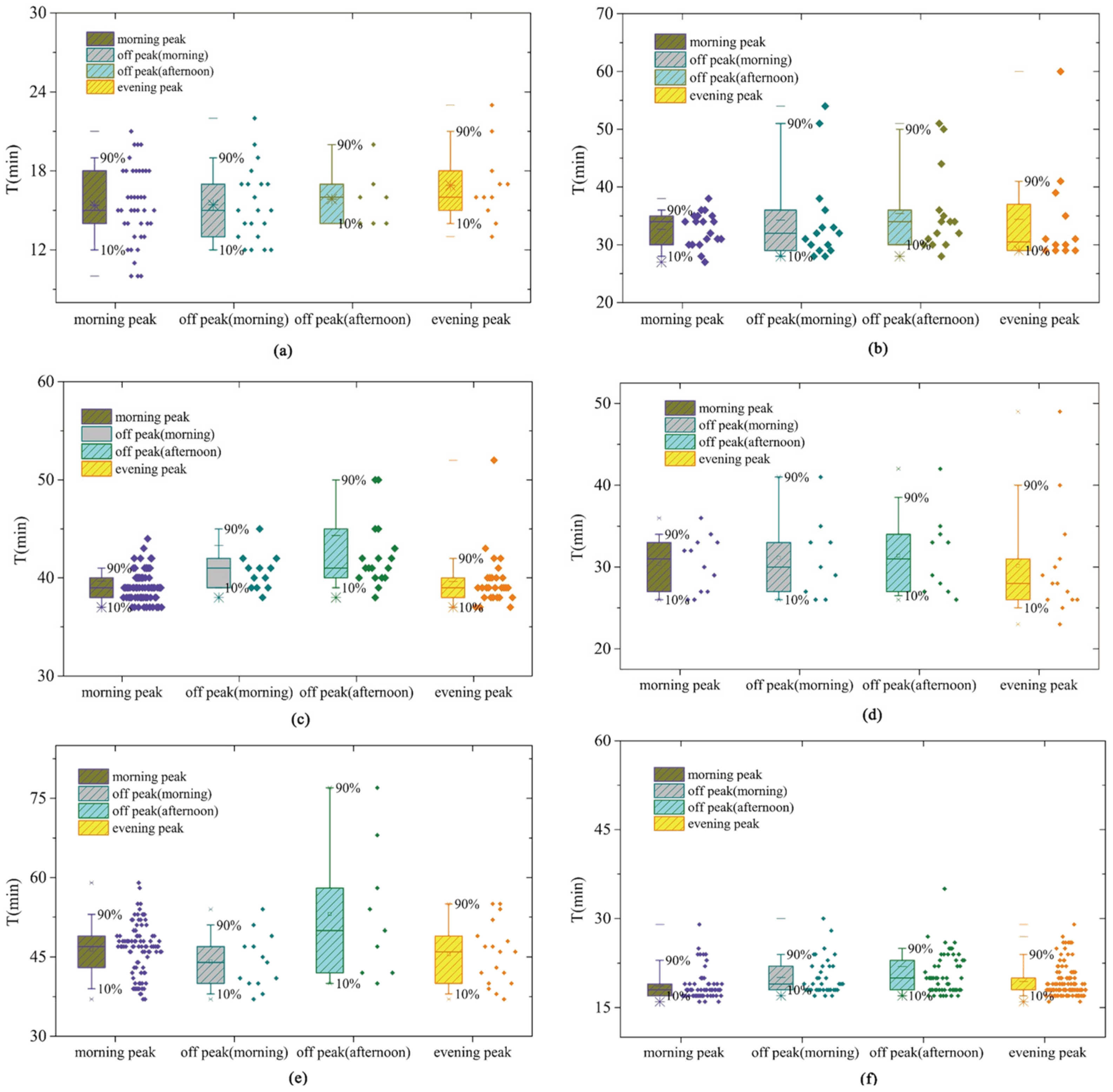
Beijing South Railway StationThird QuadrantOverall service capacity is weak; needs comprehensive improvement in bus network density.
Beijing Capital International AirportSecond QuadrantFew overall paths and uneven distribution; requires enhanced route coverage and transfer optimization.
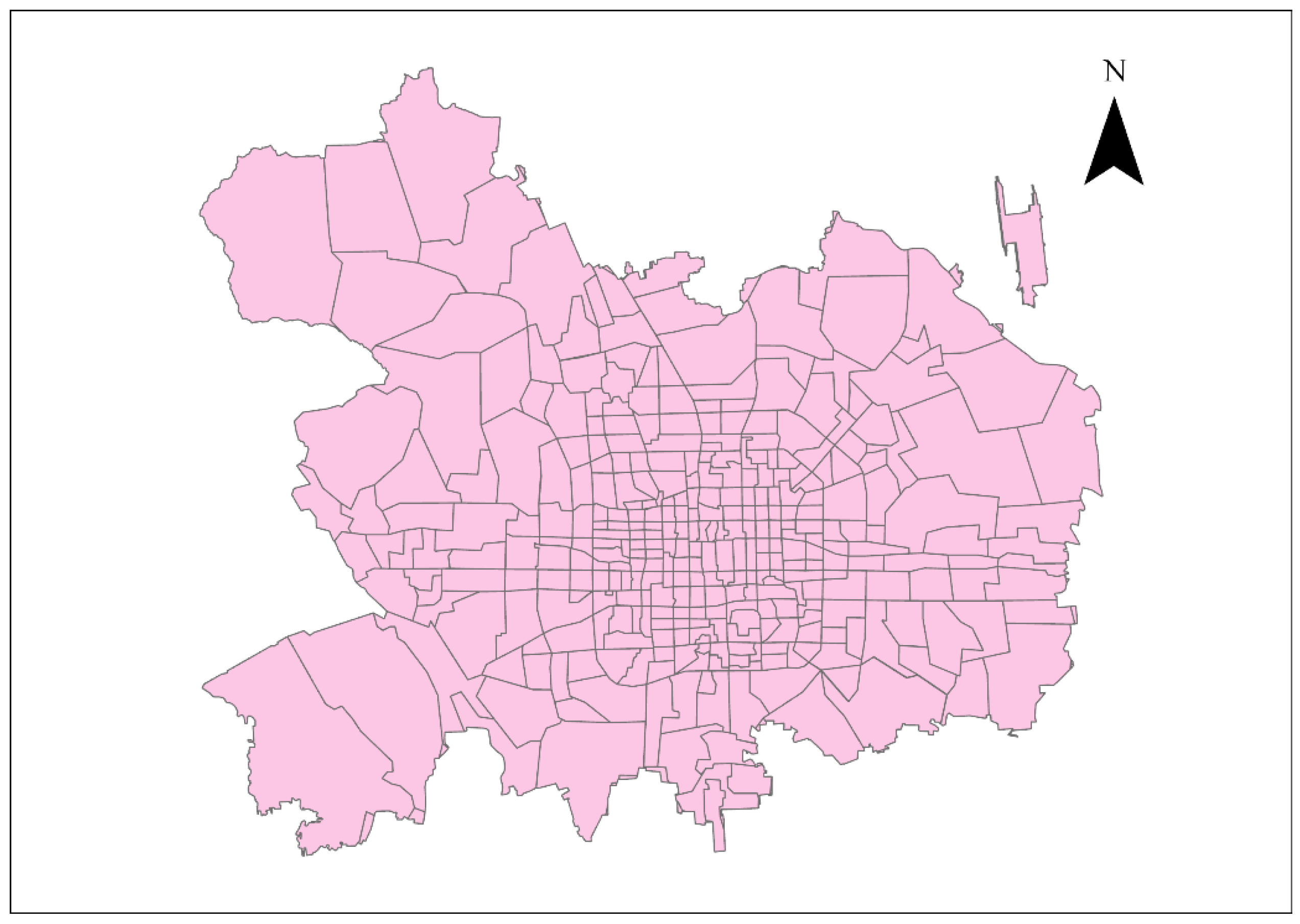
Beijing Railway StationSecond QuadrantFew overall paths and uneven distribution; requires enhanced route coverage and transfer optimization.
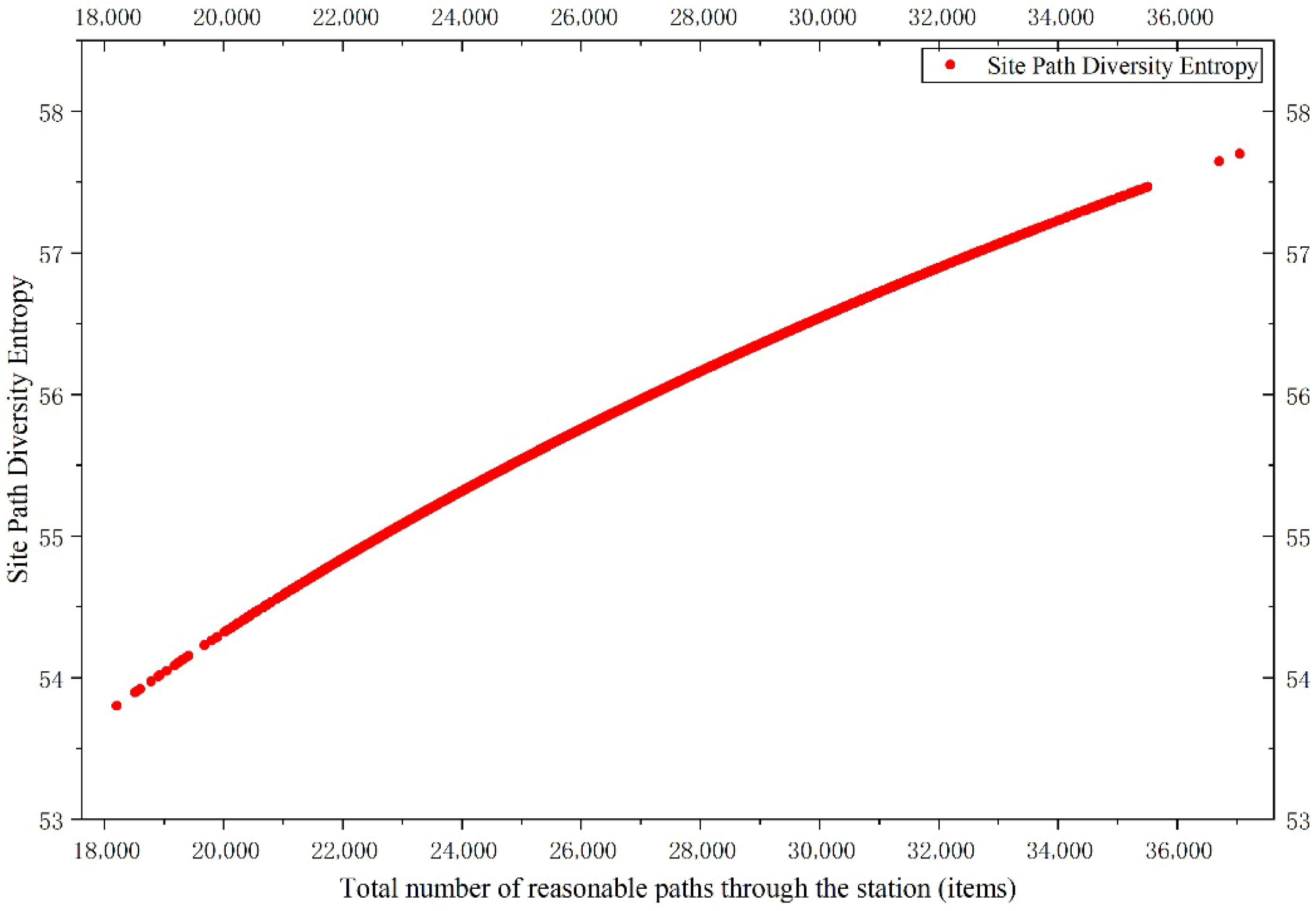
Beijing West Railway StationFourth QuadrantInternal stop path distribution is even; high passenger travel convenience.
Beijing Fengtai Railway StationFirst/Fourth QuadrantPath resources concentrated in a few stops; needs optimization of internal stop connections.
Liuliqiao Long-Distance Bus HubThird/Fourth QuadrantInternal stop path distribution is even; high passenger travel convenience.
Qinghe Railway StationFourth QuadrantInternal stop path distribution is even; high passenger travel convenience.
Disclaimer/Publisher’s Note: The statements, opinions and data contained in all publications are solely those of the individual author(s) and contributor(s) and not of MDPI and/or the editor(s). MDPI and/or the editor(s) disclaim responsibility for any injury to people or property resulting from any ideas, methods, instructions or products referred to in the content.