Thermal Performance of Earthen Architecture in Ushaiger, Saudi Arabia: A Pilot Digital-Twin Feasibility Study

Abstract

This study presents a pilot methodological investigation of the thermal performance of a Najdi mudbrick dwelling in Ushaiger, Saudi Arabia, using short-term field monitoring and a preliminary digital-twin inspired workflow. Two field campaigns in August and September 2025 measured indoor and outdoor conditions with a portable weather station under severe site constraints, including lack of electrical infrastructure, restricted access, and the use of consumer-grade sensors. The monitored results indicate that the massive earthen walls attenuated part of the outdoor daily temperature swing, but indoor conditions remained very hot: in August, indoor temperatures averaged 38.1 °C, compared with 40.2 °C outdoors, and in September, indoor temperatures averaged 36.3 °C, compared with 36.1 °C outdoors. A simplified IDA ICE model was compared with the monitored indoor temperature over the available windows, and a post-processing affine bias adjustment was tested only as a diagnostic short-window correction rather than as a transferable calibration. Monte Carlo sensitivity analysis was used in an exploratory way. It examined how passive envelope and boundary-related parameters influenced simulated indoor relative humidity, with infiltration emerging as the dominant factor affecting relative humidity dynamics; peak indoor relative humidity increased from about 67% at 0.15 air changes per hour (ACH) to more than 74% at 0.60 ACH, whereas wall thickness had a modest buffering effect. Given the short monitoring duration and field limitations, the study is not presented as a fully validated digital twin but as a feasibility-oriented workflow that combines constrained in situ monitoring with exploratory simulation to support future, longer-term conservation and adaptive reuse research on earthen heritage in hot–arid climates.

1. Introduction

Earthen architecture has long shaped cultural identity and sustainable construction in hot–arid regions. Mud brick is favored for its low embodied energy, local availability, and passive thermal performance [1]. In Saudi Arabia, heritage settlements such as Ushaiger contain clusters of earthen dwellings. These reflect traditional responses to climate, materials, and social organization. Ushaiger Heritage Village, northwest of Riyadh, has been documented and culturally recognized [2,3]. However, its material performance [4] and environmental behavior [5,6,7,8,9] have not been closely examined.

The question of human comfort in Saudi heritage buildings has gained momentum as diverse climatic zones have historically produced distinct architectural responses. Research on Hijazi architecture in Jeddah shows how thermal mass and natural ventilation, supported by Al-Mangabi stone, moderated indoor conditions in hot–humid environments, while central and eastern settlements developed courtyard houses and orientation strategies suited to dry, arid climates [10,11,12,13]. Field studies in Riyadh further indicate that adobe dwellings can reduce internal temperatures through passive strategies [14], and experiments on ventilated courtyards in central Arabia demonstrate the benefits of cross-ventilation [15]. Recent work in Jeddah’s classrooms illustrates how modern zonal air distribution can complement passive traditions [16].

Scholarship on Ushaiger and other heritage villages focuses on cultural significance, community participation, and sustainability agendas [2,17,18,19,20]. Earthen construction is now seen as a cultural asset and a model for contemporary ecological strategies. However, while these works focus on architecture and conservation, they do not address how earthen dwellings perform environmentally during the harsh summer conditions of central Arabia.

Despite a growing body of research on earthen and climate-responsive architecture, rigorous in situ monitoring of Najdi mud-brick dwellings during peak summer remains scarce. Much empirical literature focuses on Mediterranean or North African contexts or reports short campaigns and single-zone spot measurements that cannot resolve diurnal damping, time lags, cross-ventilation pathways, or envelope-driven stratification in rooms typical of Najdi houses [18,19]. Saudi studies often emphasize courtyards or coastal Hijazi settings, while central-Arabian adobe research is dated or simulation-heavy, leaving a geographic and methodological blind spot for Ushaiger and comparable settlements; this limits evidence-based guidance for conservation design, comfort targets, and retrofit strategies under today’s extreme heat [21,22].

Another gap concerns integrative methods. Few studies combine high-frequency indoor–outdoor microclimatic monitoring with precise geometric survey and physics-based building simulation in a way that allows measured and simulated behaviour to be compared under real field constraints [23,24,25]. Without such coupled datasets, it remains difficult to test passive measures against observed performance or to translate findings into evidence-based conservation strategies for the Najdi fabric. Ushaiger, although well documented culturally, still lacks this combined empirical–computational evidence base.

The present study addresses this gap through short-term empirical monitoring of an earthen dwelling in Ushaiger across two summer campaigns, supported by a CAD-based digital survey and a preliminary digital-twin workflow. This integrative approach provides an initial dataset on indoor–outdoor microclimatic dynamics in a Najdi heritage village and proposes a pilot methodological framework for future conservation analysis and adaptive-reuse studies in similar contexts. Situating the analysis within debates on thermal comfort, conservation, and sustainable reuse, the research contributes to the literature and extends prior work on Ushaiger [2,26] by offering a replicable, feasibility-oriented framework for conservation policy and adaptive-reuse strategies in similar contexts. This research is funded by Prince Sultan University (Research and Initiative Center RIC Seed Project No. 208_2025), which enabled the procurement of the initial equipment for digital-twin-oriented monitoring; however, the monitoring duration was constrained by site accessibility, unsafe building conditions, and the lack of permanent electrical power in the abandoned building, requiring a temporary power supply for the sensors.

In this study, the term ‘digital twin’ is used in a simplified, non-real-time sense to denote a geometry-based and data-linked simulation model; it does not imply continuous data synchronization, bidirectional data exchange, or control functionality [27]. Thus, the study is a pilot feasibility phase of a longer digital-twin monitoring plan for Ushaiger Heritage Village. It aims to test field deployment under real constraints and build a protocol for future campaigns. The temporary power supply (Wagan Tech Power Dome NX2) and access limits reduced the temporal continuity of measurements. Therefore, the results serve as baseline evidence to support model plausibility and to interpret hygrothermal conditions in a deteriorated dwelling. This is not a full seasonal or annual assessment. In the next project phase, monitoring will be longer and more robust with upgraded equipment and on-site power. This will enable broader evaluation of model robustness over seasonal periods.

2. Literature Review

The Kingdom’s diverse climates and regional building traditions shape comfort in Saudi heritage buildings. The five major regions—central, northern, southern, eastern, and western—developed unique massing, spatial, and material strategies. These approaches temper heat and solar gain while supporting social practices [17]. In the humid west, Hijazi dwellings rely on cross-ventilation, shading, and porous masonry to stabilize indoor conditions. Architectural studies in Jeddah’s Baeshen House demonstrate these passive techniques [11]. Cross-regional syntheses confirm that vernacular dwellings aim to control airflow, manage radiant heat, and leverage thermal inertia. However, their quantitative performance varies by local conditions and occupancy patterns [28,29].

The Arid Najdi and Gulf contexts evolved distinct repertoires. Courtyard houses with optimized orientations, thick adobe envelopes, and controlled apertures reduce conductive and radiant gains while supporting buoyancy-driven airflow; classic measurements in a Riyadh-area test house showed that a ventilated interior courtyard measurably cools adjacent spaces under peak summer loads [15]. Recent outdoor–indoor studies on courtyard orientation indicate that geometry and exposure materially affect air temperatures and cooling demand in school compounds, reinforcing the transferability of courtyard intelligence to contemporary programs [3,30]. At the envelope scale, thermal-mass sensitivity analyses using Saudi reference climates demonstrate that wall heat capacity and diffusivity can shift cooling energy significantly, clarifying when mass helps or penalizes demand in hot regions [31,32].

Field evidence from Riyadh adobe houses underscores the potential and limits of passive operation. Monitoring and simulation of traditional dwellings showed average indoor air temperatures 4–6 °C below outdoors and peak dampening up to 12 °C when night purging and courtyard evaporative conditioning were actively managed, suggesting that this performance depended on precise ventilation timing and moisture sources rather than on fabric mass alone [14]. Complementary work in historic Jeddah demonstrated that combining mashrabiya (lattice windows) with evaporative techniques elevates airflow and reduces operative temperatures during extreme summer periods, illustrating hybridization paths that respect heritage morphology [33]. Across earthen typologies, new studies link material physics to building-scale outcomes: hygrothermal monitoring and enhancement of rammed earth in hot climates connect lab properties to in situ behaviour [34], while compressed-earth case studies report seasonal buffering and intra-wall moisture–conductivity coupling with comfort implications [35].

Moreover, current work (

Table 1. Recent IDA-ICE studies.

Reference	Location/Type	IDA-ICE Focus	Key Finding/Relevance
[36]	Sweden, multi-storey housing	Overheating assessment with IDA-ICE 4.8	Demonstrates IDA-ICE for floor/orientation sensitivity under present and future climates; strong template for overheating metrics.
[37]	Nordics, decarbonization scenarios	Zero-emission actions simulated in IDA-ICE	Uses IDA-ICE to quantify energy-saving actions toward zero-emission targets; evidences tool’s policy-relevant scenario analysis.
[38]	Europe, office test case	Hygrothermal modelling; IDA-ICE with 1D HAM wall	Shows thermal model in IDA-ICE and HAM wall coupling for hygrothermal response; method relevant for moisture-active earthen envelopes.
[39]	Mixed climates; field + simulation	Operating building analysis using IDA-ICE inputs	Details IDA-ICE building inputs and compares with measured data; supports monitoring–simulation coupling approach.
[40]	Cold climate; retrofitted glazing	Energy and indoor climate with added glazing	Early but foundational IDA-ICE use to quantify glazing retrofits; relevant to solar-gain control and overheating.
[41]	Highly glazed spaces	IDA-ICE 4.61 glazed-space thermal simulation	Establishes IDA-ICE suitability for detailed solar/thermal behaviour in glazed spaces; informs SHGC and shading scenarios.

) confirms IDA-ICE as a validated dynamic simulation platform across climates and applications, including overheating assessment, zero-emission scenario design, hygrothermal modelling with Heat, Air, and Moisture (HAM) extensions, and mixed field–simulation studies. Studies deploy IDA-ICE for indoor overheating risk and mitigation, system-level retrofits, and bias-adjusted building analyses, while earlier research established its suitability for glazed-space physics and envelope sensitivity. Despite this breadth, to our knowledge, no study couples IDA-ICE with in situ monitoring of Najdi mud-brick dwellings, underscoring the need for a Saudi heritage case with empirical grounding.

Sustainability framings have advanced in parallel [42,43]. Life-cycle assessments increasingly position earthen construction as a low-impact alternative, quantifying the benefits and trade-offs of stabilized rammed earth and fibre-reinforced earthen construction relative to conventional assemblies [6]. Whole-building hygrothermal analyses show climate-dependent limits, cautioning against one-size-fits-all prescriptions for raw-earth monolayer walls [44]. These material-level insights complement broader reviews calling for measured datasets and standardized protocols to bridge simulation and reality in earthen buildings [24].

A substantive gap persists for Najdi earthen settlements. Research on Ushaiger has largely focused on its cultural importance, conservation methods, and reuse for tourism, but little attention has been given to how its buildings actually perform under extreme summer conditions. There is still no detailed monitoring of indoor and outdoor climates in Najdi mud-brick houses, whether inhabited or partly abandoned. Understanding how heat, humidity, air movement, and courtyards interact in these settings is crucial, yet systematic evidence is missing. Without such knowledge, strategies for reuse, comfort improvement, and conservation in central Arabia remain vague and incomplete.

To address this shortcoming, the present study combines field measurements with digital analysis to examine the environmental behaviour of a Ushaiger earthen dwelling during summer. Continuous monitoring of temperature, humidity, and air movement is paired with detailed CAD-based surveys and a digital-twin workflow that aligns observations with physics-based simulations. This approach generates a high-resolution dataset tied to spatial form and material properties, while also demonstrating how bias-adjusted models can inform conservation guidelines and support low-energy reuse strategies for Najdi mud-brick architecture.

Within this framework, the study is guided by the following research questions:

• RQ1: How do indoor temperatures and relative humidity in a Ushaiger mud-brick dwelling behave during peak summer compared with outdoor conditions, and what level of diurnal damping and time lag do the earthen walls provide?
• RQ2: How can the combination of on-site monitoring and a simplified IDA ICE model test the feasibility of a preliminary digital-twin workflow to support future conservation and adaptive-reuse strategies for Najdi mud-brick houses?

3. Methodology

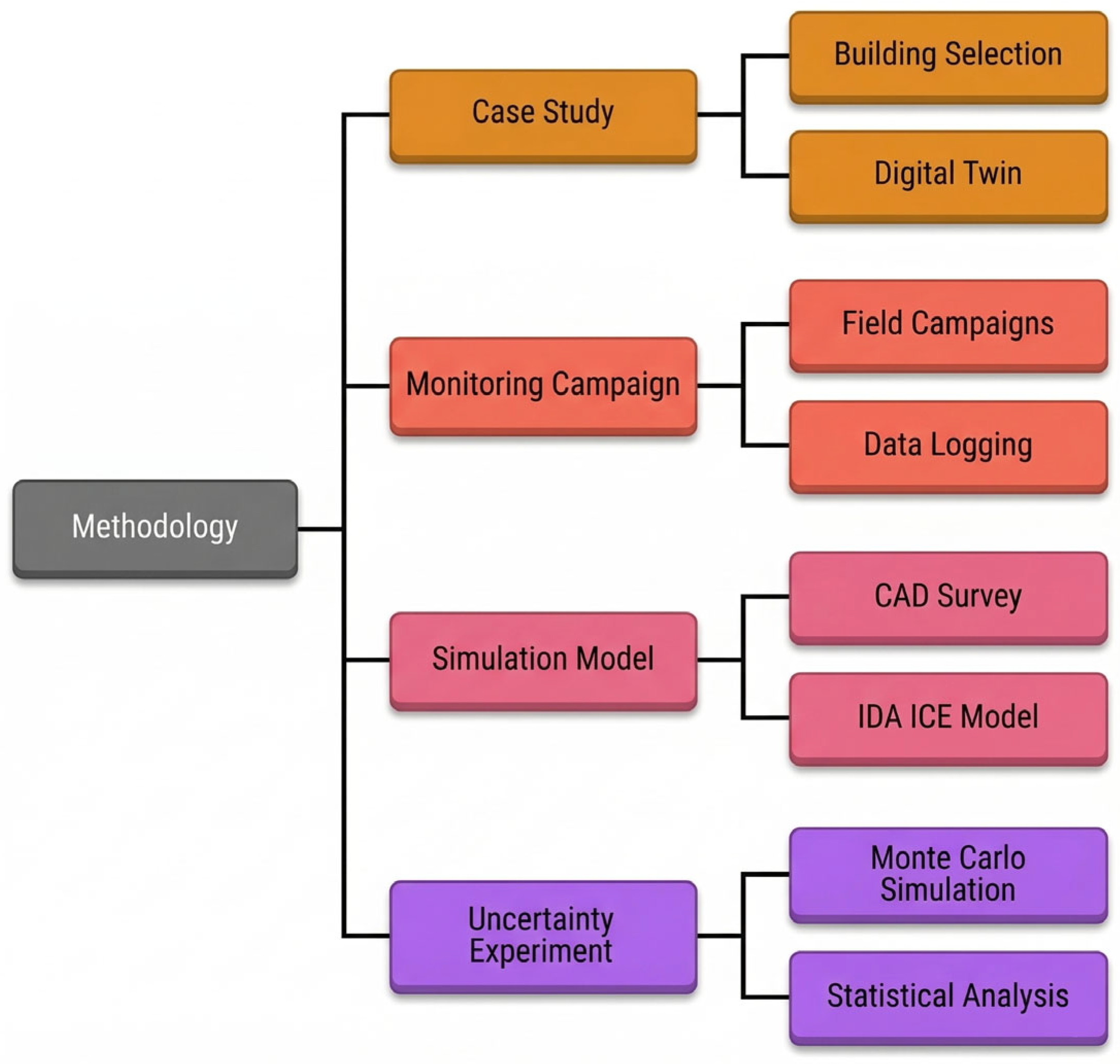
The research followed a multi-step methodology (Figure 1) combining empirical monitoring, digital modelling, and statistical analysis to assess the thermal performance of a mud-brick dwelling in Ushaiger. The process began with selecting a representative case study and developing a digital twin. Field campaigns were then conducted to collect high-resolution environmental data, both indoor and outdoor.

A CAD-based survey was used to reconstruct the building geometry, which was implemented in IDA ICE to create a simulation model aligned with measured conditions. Finally, a Monte Carlo sensitivity analysis was performed to examine how passive envelope and boundary-related parameters influenced RH-related simulation outputs, particularly maximum indoor relative humidity (MaxRH). This integrated workflow ensured both empirical grounding and computational robustness for evaluating the performance of earthen architecture under extreme climatic conditions.

3.1. Case Study: The Ushaiger Mud Brick Dwelling

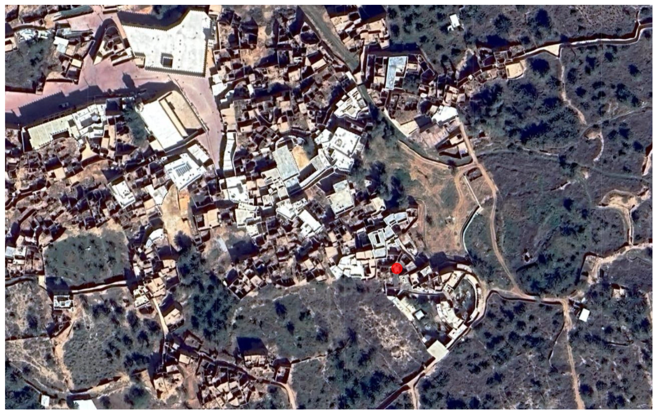
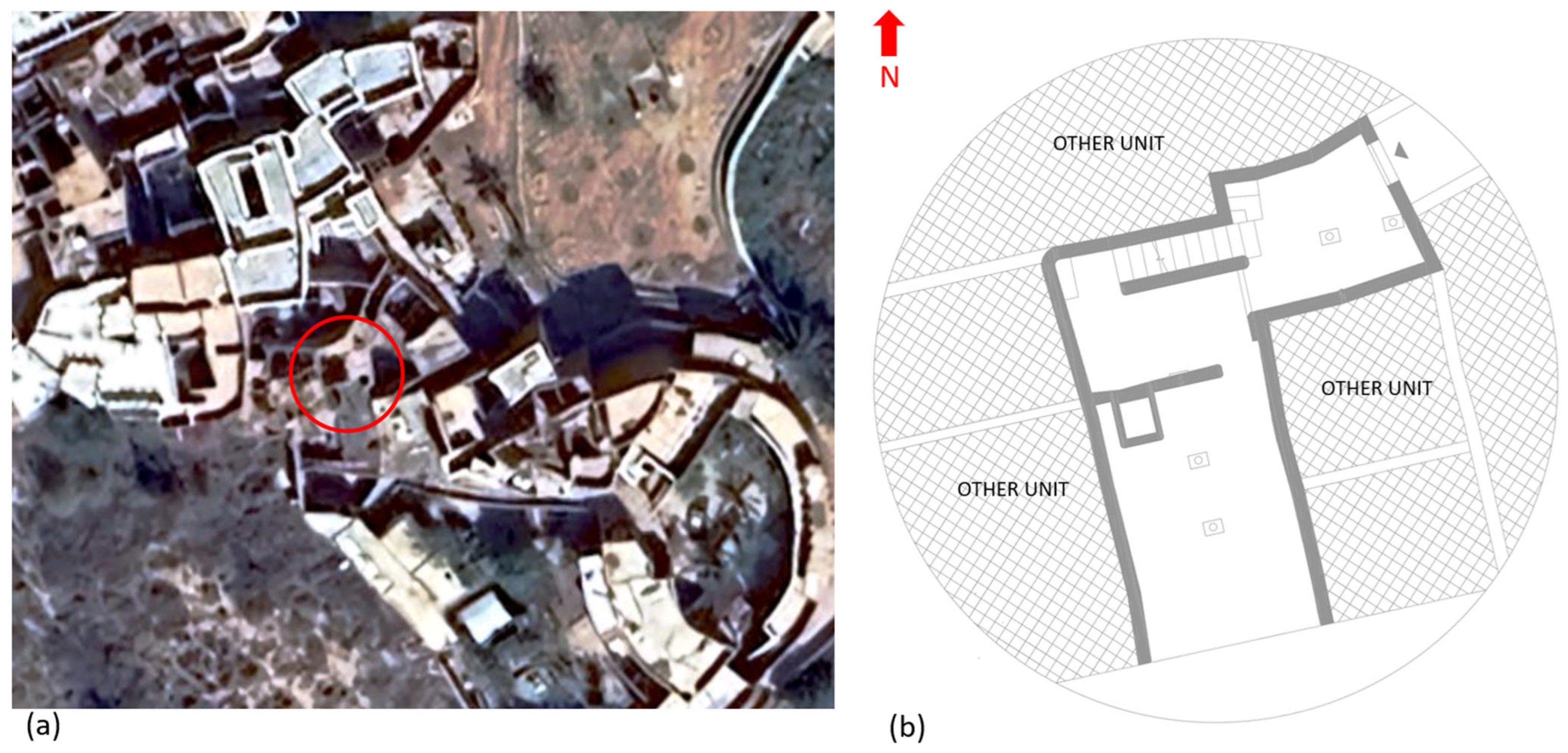
The building selected for monitoring is situated at coordinates 25.3384° N and 45.1946° E, within the central nucleus of Ushaiger Heritage Village (Figure 2). The structure is partially abandoned and has lost its electrical connection, a condition common across the village. Constructed of traditional mud bricks, the dwelling features massive earthen walls, a flat rooftop, and a modest footprint consistent with Najdi vernacular architecture. Documentation of the building’s geometry and orientation was undertaken through a three-dimensional CAD survey, which was then elaborated into a digital twin model used to represent the building’s as-found condition and to support exploratory simulation under the monitored field conditions. The digital model was linked to environmental monitoring, providing a framework for interpreting performance data and ensuring alignment between observed and simulated behaviours.

The broader assessment of Ushaiger’s building stock indicates that many of the village’s structures are in fragile states of preservation, ranging from partially collapsed to only partially in use, with conservation levels often rated between average and poor. The dwelling analysed in this study corresponds to a portion of a larger compound recorded in the survey, representing the typical conditions of partially abandoned houses where earthen walls survive but roofs and plaster are in an advanced state of decay. Such structures, while compromised, retain enough integrity to offer valuable opportunities for monitoring and experimentation.

The selection of this particular case study was motivated by several factors that underline its significance for future reuse strategies. First, the house embodies the common typology of many neglected dwellings in Ushaiger, making it a representative pilot for performance monitoring and conservation-oriented interventions. Second, its location adjacent to the settlement’s agricultural fringe emphasizes the historic interdependence between domestic architecture and subsistence practices, which were essential to the survival of the inhabitants. Third, and most importantly, the dwelling is linked to instances of community participation in restoration work, where local residents have demonstrated a strong inclination to reuse existing structures in spontaneous, incremental ways. This bottom-up engagement, observed during restoration efforts across the village, provides a critical framework for envisioning sustainable reuse strategies that balance authenticity with contemporary needs.

By anchoring the analysis in measured indoor and outdoor conditions, this study seeks to inform practical proposals for adaptive reuse that address current climatic pressures while preserving the social significance of heritage. The chosen dwelling, positioned between abandonment and reuse, illustrates how earthen architecture can simultaneously embody cultural memory and function as a testing ground for preservation and reuse approaches oriented toward the future.

3.2. Monitoring Campaign

Monitoring was conducted in two field campaigns, the first in early August 2025 during peak summer conditions and the second in early September 2025 under slightly milder outdoor conditions. Because the dwelling lacked permanent electrical infrastructure, all instruments were powered by a Wagan Tech Power Dome NX2 portable supply, manufactured by Wagan Corporation (Hayward, CA, USA), and sourced in Riyadh, Saudi Arabia. Measurements were obtained with a Netatmo Smart Weather Station, composed of one outdoor module and two indoor modules, linked wirelessly to a central logger, enabling almost continuous recording with occasional gaps. The monitoring duration was constrained by site conditions typical of partially unsafe heritage buildings with limited infrastructure: electrical power was available only via a rechargeable battery with limited autonomy, and access to the dwelling was restricted for safety reasons to a small number of operators. These constraints influenced the achievable temporal coverage of each campaign and explain why the dataset is organized in short monitoring windows. This strategy was adopted to establish a safe, repeatable protocol under real field conditions as a preparatory step for longer deployments in subsequent project phases. Figure 3 illustrates the location of the selected dwelling in Ushaiger village and the ground-floor plan of the monitored building and adjacent units.

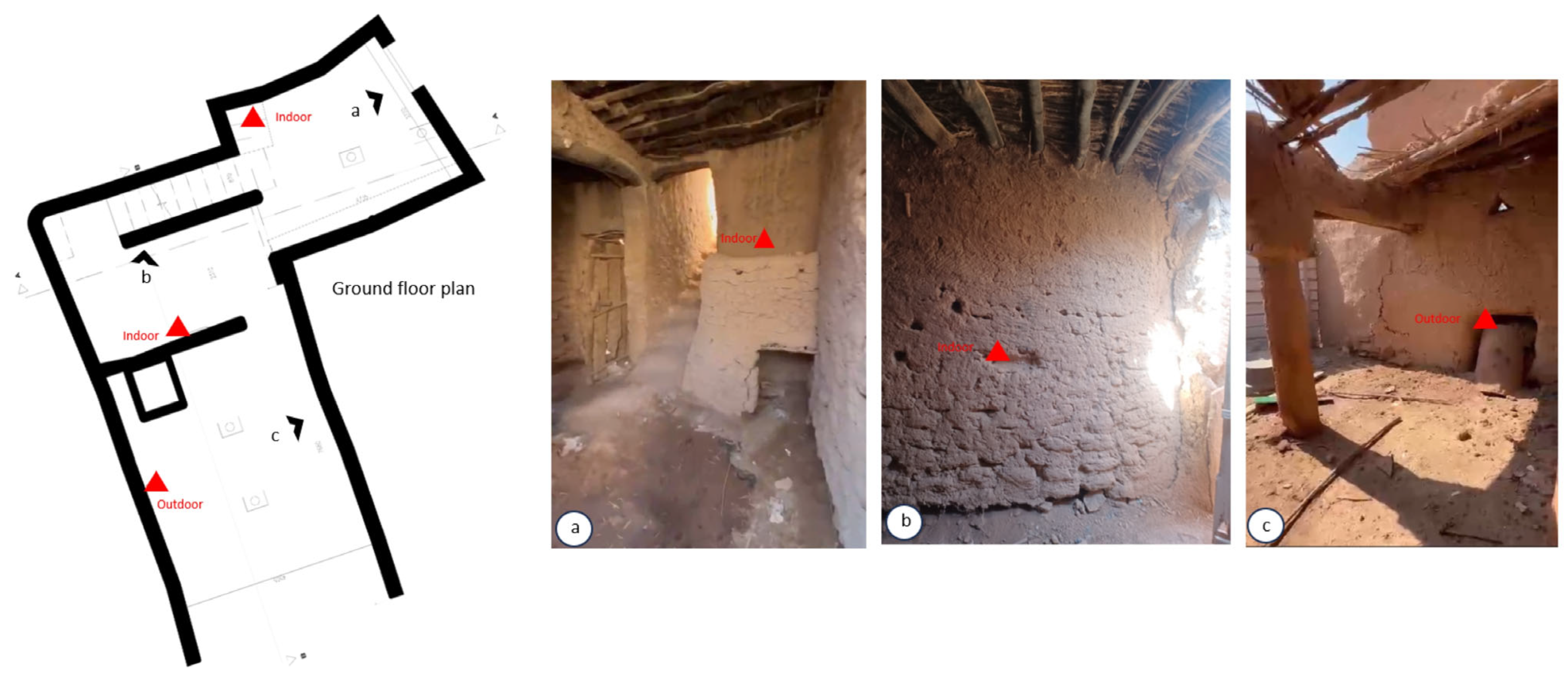
The monitored parameters included air temperature, relative humidity, barometric pressure, carbon dioxide concentration, and noise level. According to manufacturer specifications, the sensors achieve an accuracy of ±0.3 °C for temperature, ±3% for relative humidity, ±5% for CO₂, ±1 mbar for pressure, and ±3 dB for sound level. Data were logged at five-minute intervals for several consecutive days in each campaign, producing a high-resolution dataset that captured both diurnal cycles and short-term fluctuations. The indoor probe was positioned at approximately 1.5 m above the floor in the main intact room of the dwelling, representing breathing-zone height. The first indoor module was positioned close to the wall opposite the main entrance, mounted above an earthen protruding element to provide a stable and representative indoor reading. The second indoor module was placed in an adjacent space to confirm spatial consistency, close to the wall. The indoor temperature and relative humidity values reported in this paper refer to the primary indoor module located in the main intact room. The second indoor module was used solely as a qualitative cross-check of spatial consistency and was not averaged with or used interchangeably with the primary indoor series, because the two sensors were installed in distinct micro-locations within the dwelling. The outdoor sensor was mounted in a shaded, well-ventilated position in the courtyard, ~1.0 m above ground level, near the façade, and sheltered from direct solar radiation and wall reflections. All the Netatmo modules were installed on the ground floor, as indicated in the ground floor plan in Figure 4.

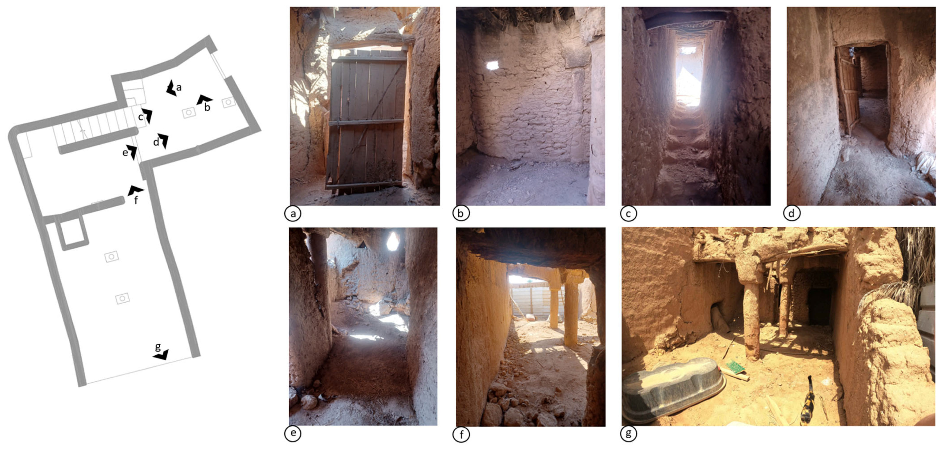
The selected dwelling unit represents a highly degraded, non-serviced earthen structure typical of the still-unrestored buildings in Ushaiger. As documented in Figure 5, the building exhibits advanced decay, including missing door leaves and incomplete closures at openings (Figure 5a,d), eroded and cracked earthen wall surfaces (Figure 5b,e), and localized collapses and damaged transition spaces that increase exposure between interior rooms and the courtyard/exterior (Figure 5c,f,g). The intent of this study is therefore not to represent an “ideal restored” house, but to characterize indoor–outdoor hygrothermal behaviour under the as-found condition, establish a baseline to quantify the buffering potential of earthen fabric and passive strategies, and inform future restoration scenarios and longitudinal monitoring.

The raw data were exported for processing, and outliers caused by power interruptions or sensor resets were removed. Gaps shorter than 15 min were interpolated, and the cleaned dataset was resampled to hourly means for analysis, while the original five-minute records were retained for verification.

Instrumentation and Data Quality

The monitoring system was selected to operate under restricted access and limited electrical infrastructure in a deteriorated heritage dwelling. The deployed sensors are consumer-grade devices; therefore, the measurements should be interpreted as indicative of relative behavioural trends, and potential measurement bias may affect both absolute values and the apparent level of agreement between monitored and simulated results.

Therefore, the measurements should be interpreted as supporting comparative behavioural analysis within the monitored windows rather than as reference-grade observations suitable for rigorous absolute validation. Manufacturer-stated sensor performance is reported in

Table 2. Instrumentation overview and uncertainty reporting for the pilot monitoring campaign.

Instrument	Variables	Sampling and Aggregation Used in This Study	Uncertainty Reporting Approach	Placement and Notes
Netatmo indoor module	Temperature, RH	Native sampling aggregated to hourly means	Manufacturer-stated performance reported, no reference co-location in this phase	Indoor sensor location described in text and shown in Figure 4
Netatmo outdoor module	Temperature, RH	Native sampling aggregated to hourly means	Manufacturer-stated performance reported	Placed in shaded, ventilated location to reduce radiative bias where feasible
Portable power supply	Power continuity	Battery-based	Data gaps documented	Limited power duration constrained monitoring window length

, but no reference-grade co-located calibration or validation was feasible within the present field constraints. Accordingly, the dataset is used primarily to capture short-term indoor–outdoor dynamics, relative temporal patterns, and comparative differences between monitored and simulated behaviour, rather than to claim laboratory-grade absolute accuracy [1,35]. Data processing included time-based harmonisation, removal of clearly spurious spikes, and documentation of missing-data gaps. For this reason, the monitored data are interpreted mainly as evidence of relative behavioural trends and short-window model plausibility, rather than as a basis for high-precision absolute performance verification.

To ensure transparency in data quality, all timestamp discontinuities were quantified during preprocessing. Short gaps (≤15 min) were treated as brief transmission losses and were filled using linear interpolation, as described above. Longer gaps (>15 min) were not interpolated and were retained as missing data to avoid introducing artificial trends; analyses and model-affine adjustment of the simulated temperature series were therefore performed only on the continuous monitoring windows available. In the dataset, 3 indoor and 5 outdoor gaps longer than 15 min were identified. These include one shared long interruption consistent with a temporary loss of station connectivity/power affecting both modules, as well as shorter outages. Reporting these occurrences clarifies the effective usable monitoring duration and supports a conservative interpretation of the short monitoring campaign.

The processed dataset provided the basis for analysing indoor–outdoor thermal dynamics, relative humidity behaviour, and the extent of diurnal lag and damping attributable to the adobe envelope. CO₂ levels were used to verify the building’s very low occupancy and to assess ventilation effectiveness, while pressure and noise data supported a contextual understanding of environmental events.

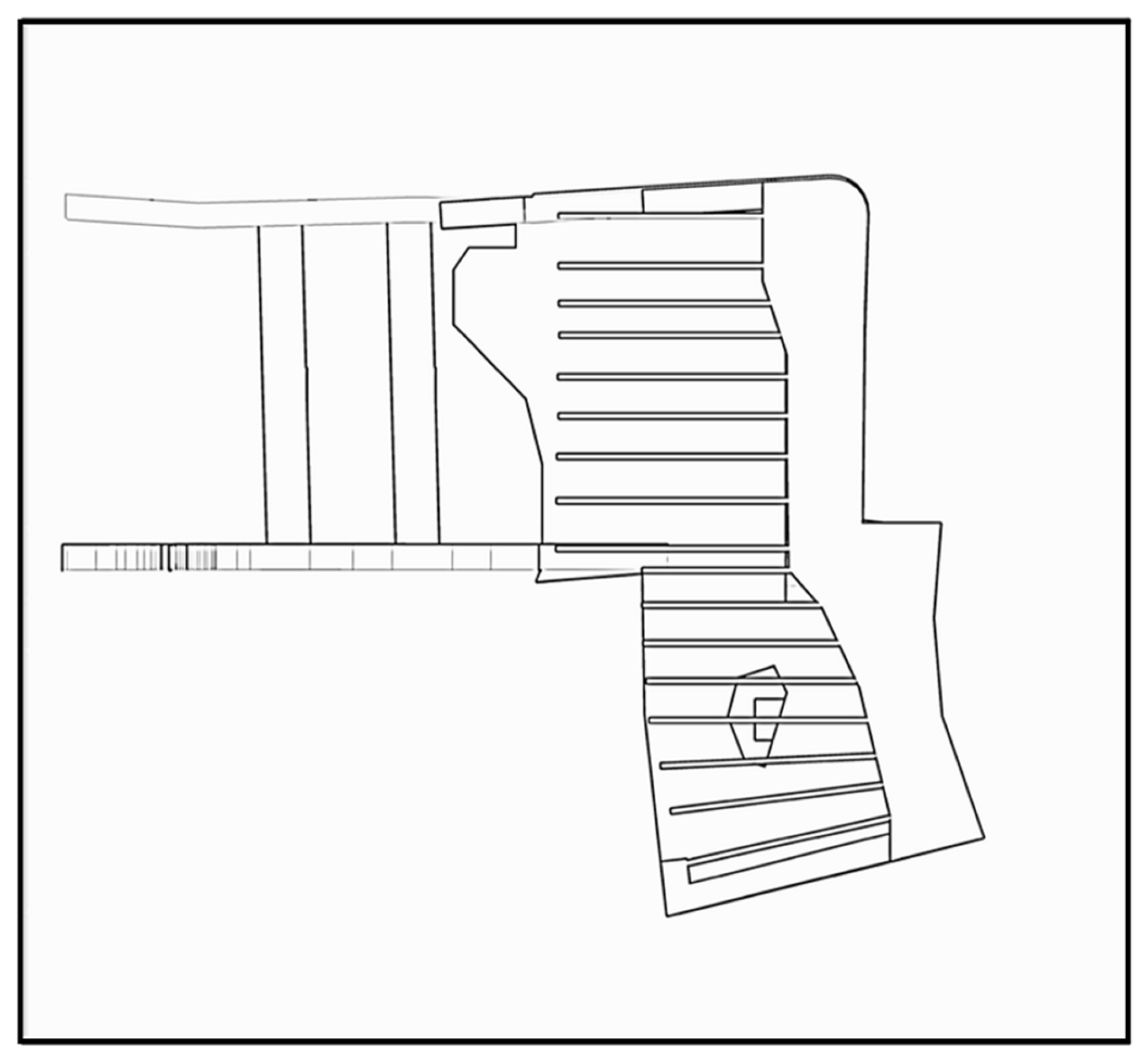
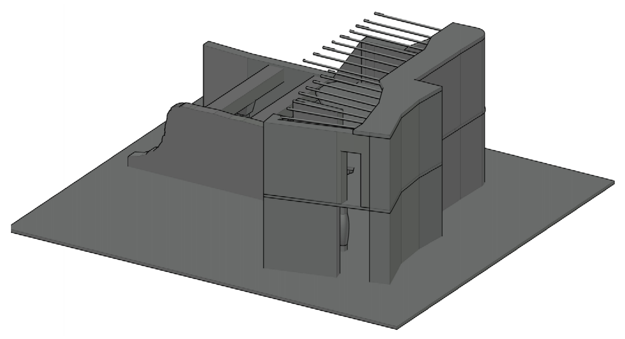
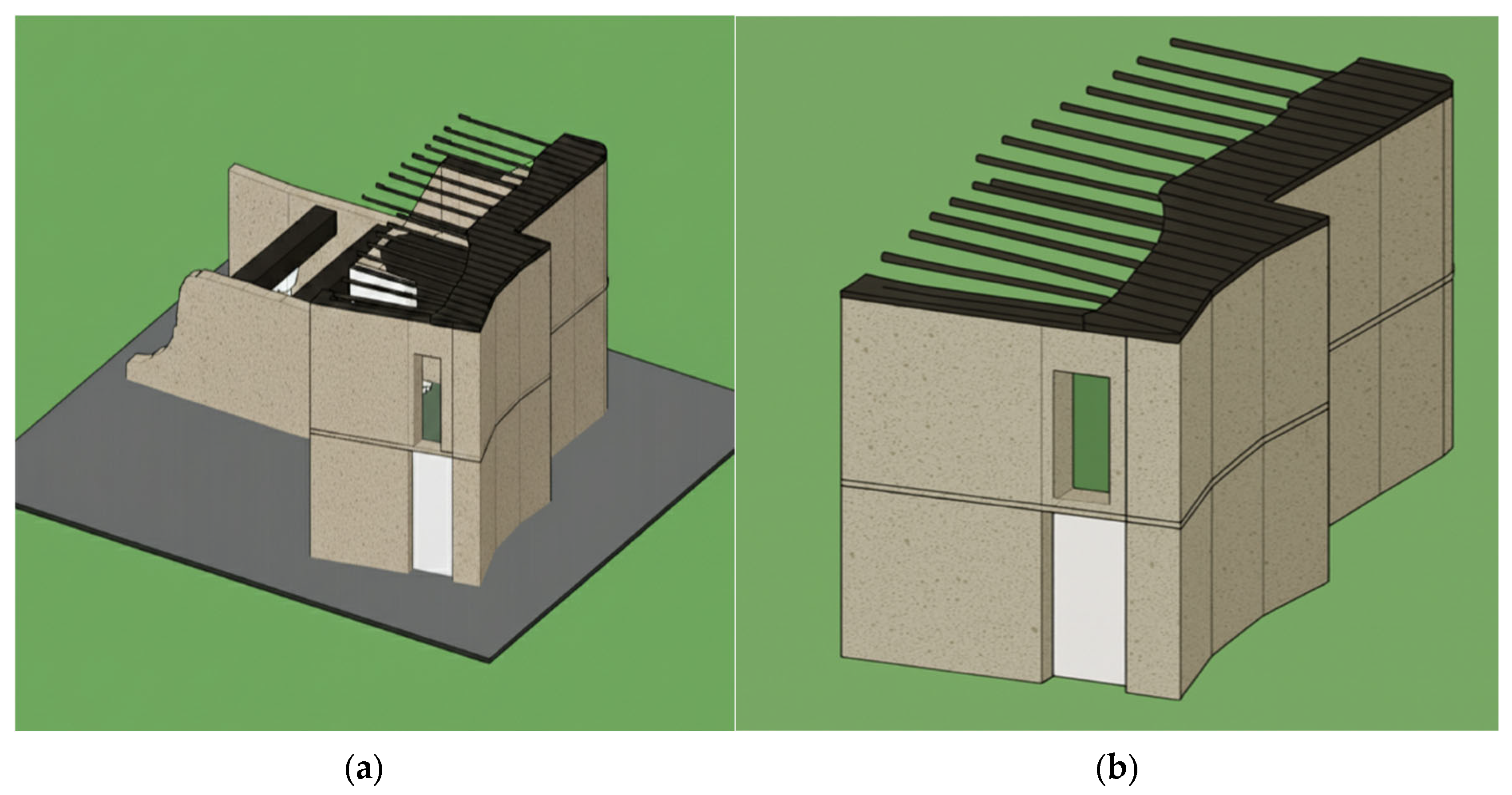
A CAD-based digital survey was undertaken to reconstruct the geometry, wall thickness, and spatial configuration of the dwelling (Figure 6). From this, a three-dimensional volumetric model was produced (Figure 7) that illustrates the envelope stratification and the house’s overall form. Thus, the study uses these CAD models to serve as the first stage of a digital twin: a geometry-based digital representation of the dwelling directly linked to the monitoring campaign. At this stage, the twin serves primarily as a documentation and visualization tool, ensuring that sensor locations, monitored zones, and envelope properties are clearly referenced. In later steps of the methodology, this geometric twin serves as the basis for developing a simplified simulation model in IDA ICE, enabling the integration of empirical data and scenario testing.

3.3. Simulation Model Development in IDA ICE

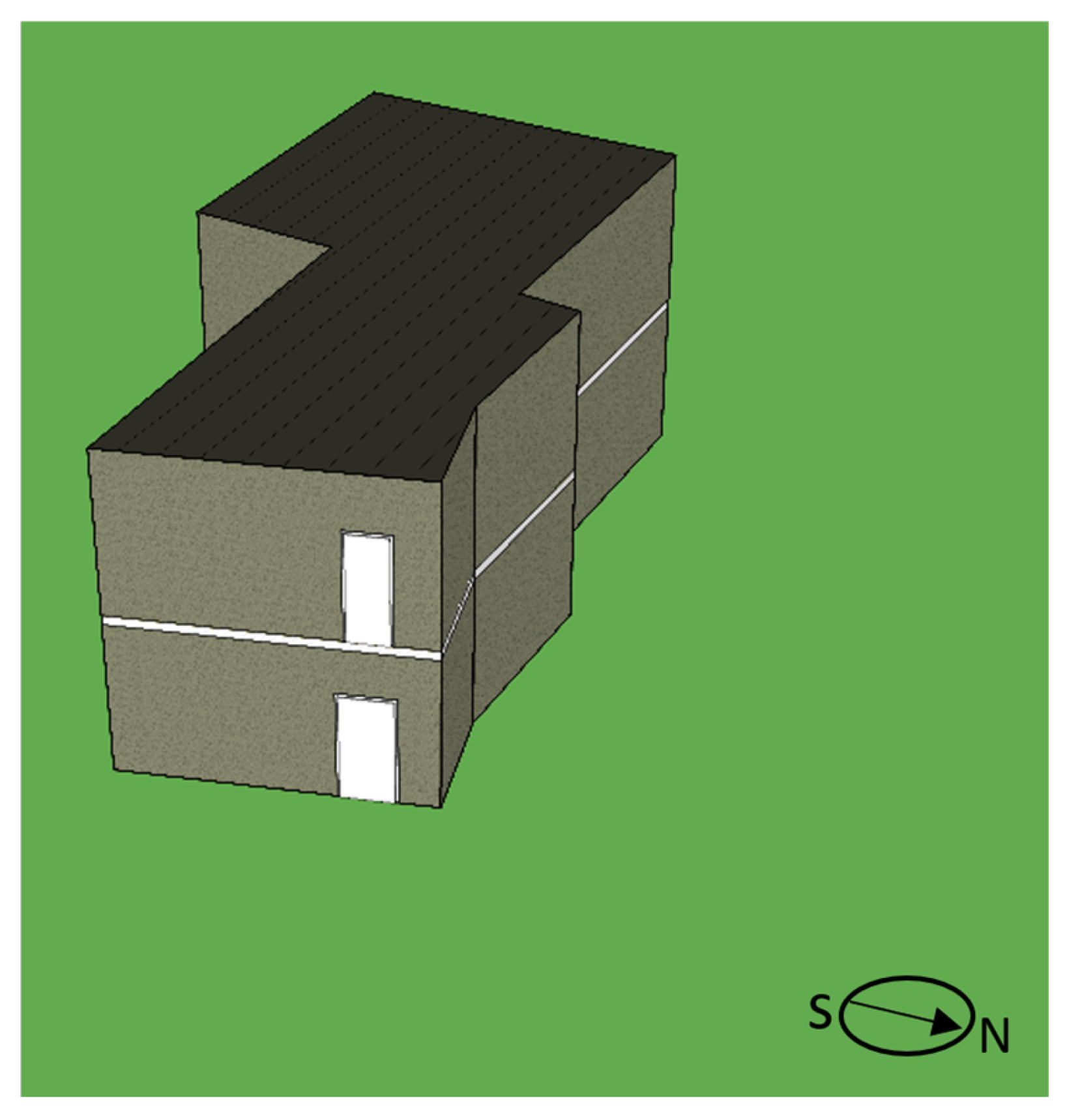
The CAD survey was converted into a three-step simulation geometry: full compound, extracted intact wing, and a minimal volumetric model aligned directly with the instrumented rooms. Collapsed or uncertain volumes were removed. Orientation and façade window-to-wall ratios were preserved within ±3%, while total floor area and internal volume were within ±5%. Two thermal zones were defined, representing the ground and upper floors, each with a floor-to-ceiling height of 3.0 m; the upper floor is elevated 3.0 m above ground, with inter-zone coupling occurring through the floor–ceiling interface.

Reconstruction Assumptions and Evidence Traceability

The as-found condition of the dwelling includes degraded or incomplete openings and partially deteriorated building elements. The digital model, therefore, includes explicit assumptions and reconstructions.

Table 3. Reconstructed and assumed elements in the as-found digital model and associated uncertainty handling.

Element or Feature	Evidence Basis	Model Representation	Uncertainty Treatment in This Study
Missing door leaves and incomplete closures	Site photos and survey notes	Opening geometry represented, closure simplified for numerical stability	Effect represented primarily through infiltration uncertainty range
Damaged window conditions	Site survey and photos	Window areas and locations retained	Sensitivity through infiltration and solar related parameters
Roof discontinuities or gaps	Site photos and observations	Simplified roof continuity in model	Discussed as structural modelling limitation, tested indirectly via infiltration range
Collapsed or inaccessible volumes	Safety constraints, limited access	Excluded from conditioned volume or idealised boundary	Documented in limitations, impact assessed qualitatively
Internal moisture and latent gains	Assumed free-running, no occupancy	Set to low or zero gains depending on period assumptions	Identified as limitation for RH interpretation
Natural ventilation behaviour	Observational	No mechanical control, free-running	Infiltration treated as key uncertain driver

documents each assumed or reconstructed element, the evidence basis used, the modelling representation, and how uncertainty is handled in the analysis. Earthen material properties were adopted from the literature due to restricted site access and the inability to extract specimens for laboratory testing. Since Adobe properties vary with density and moisture content, key envelope parameters are treated as uncertain inputs in the sensitivity and uncertainty analysis, and conclusions are bounded accordingly.

External walls were modelled using a custom Adobe material (mud brick) with thermal properties.

$$\mathsf{\lambda }=0.65 \mathrm{W} {\mathrm{m}}^{-1}{\mathrm{K}}^{-1},\hspace{1em}\mathsf{\rho }=1700 \mathrm{kg}{\mathrm{m}}^{-3},\hspace{1em}{\mathrm{c}}_{\mathrm{p}}=1000 \mathrm{J} \mathrm{k}{\mathrm{g}}^{-1}{\mathrm{K}}^{-1}$$

To support the interpretation of indoor relative humidity and to document hygrothermal assumptions, representative water-vapour diffusion resistance factors (μ) were also considered for the main envelope materials. Since no in situ cup-test characterization was possible for the studied dwelling, μ-values were adopted from published reference ranges for earthen/clay-based materials and common renders: unfired earthen/clay units can span μ ≈ 3–7 (wet-cup) and μ ≈ 7–9 (dry-cup), while unfired clay bricks reported in the literature can reach μ ≈ 10.6–23.1 depending on density and test direction; therefore, a conservative constant μ = 7 was assumed for the adobe layer, in the lower-to-mid range, for transparency in Relative Humidity (RH)-related interpretation. For renders, literature-based reference values were used as indicative bounds, consistent with standard building-physics datasets; the assumed μ-values adopted in the model are reported in Table 4. These hygric assumptions clarify the basis for RH-related interpretation, while acknowledging that future work should measure site-specific vapour diffusion resistance and moisture-storage properties for fully coupled hygrothermal modelling.

The baseline wall consists of 0.50 m adobe without plaster layers, consistent with the exposed façades observed on site. Thermal transmittance was verified analytically according to EN ISO 6946 [45] (thermal resistance and thermal transmittance calculation method):

$$\mathrm{U}={\displaystyle \frac{1}{{\mathrm{R}}_{\mathrm{s}\mathrm{i}}+\sum \left(\frac{{\mathrm{d}}_{\mathrm{i}}}{{\mathsf{\lambda }}_{\mathrm{i}}}\right)+{\mathrm{R}}_{\mathrm{s}\mathrm{e}}}}$$

$$\mathrm{with} {\mathrm{R}}_{\mathrm{s}\mathrm{i}}=0.13,{\mathrm{R}}_{\mathrm{s}\mathrm{e}}=0.04 {\mathrm{m}}^2\mathrm{K}/\mathrm{W}$$

For a single Adobe layer with

$$\mathrm{d}=0.50 \mathrm{m},\hspace{1em}\mathsf{\lambda }=0.65$$

The resistance is

$${\mathrm{R}}_{\mathrm{layer}}={\displaystyle \frac{0.50}{0.65}}=0.769 {\mathrm{m}}^2\mathrm{K}/\mathrm{W}$$

and the total resistance is

$${\mathrm{R}}_{\mathrm{tot}}=0.13+0.769+0.04=0.939 {\mathrm{m}}^2\mathrm{K}/\mathrm{W}$$

which yields

$$\mathrm{U}={\displaystyle \frac{1}{0.939}}=1.065 \mathrm{W}/{\mathrm{m}}^2\mathrm{K}$$

in agreement with the IDA ICE calculation. The corresponding specific heat capacity is

$${\mathrm{C}}^{\prime }=\sum \left(\mathsf{\rho }\hspace{0.17em}{\mathrm{c}}_{\mathrm{p}}\hspace{0.17em}\mathrm{d}\right)=1700\times 1000\times 0.50=850 \mathrm{k}\mathrm{J}/{\mathrm{m}}^2\mathrm{K}.$$

The roof construction was modelled as an earthen slab on palm trunks, consisting of four layers: an interior render of 0.01 m (λ = 0.70 W/m K), a palm-wood deck of 0.05 m (λ = 0.14 W/m K), an earthen layer of 0.22 m (λ = 0.80 W/m K), and an exterior render of 0.01 m (λ = 0.70 W/m K). Using surface resistances ${\mathrm{R}}_{\mathrm{s}\mathrm{i}}=0.10 {\mathrm{m}}^2\mathrm{K}/\mathrm{W},\hspace{1em}{\mathrm{R}}_{\mathrm{s}\mathrm{e}}=0.04 {\mathrm{m}}^2\mathrm{K}/\mathrm{W}$, the calculated values are

$$\mathrm{U}=1.25 \mathrm{W}/{\mathrm{m}}^2\mathrm{K},\hspace{1em}{\mathrm{C}}^{\prime }=448 \mathrm{k}\mathrm{J}/{\mathrm{m}}^2\mathrm{K}$$

This construction applies only to the upper zone, while the ground floor ceiling is treated as the inter-zone interface.

The ground-contact slab was modelled in accordance with EN ISO [46] as an uninsulated construction: an interior clay–lime render of 0.02 m, compacted earth/gravel of 0.10 m, and soil. Soil properties were set as

$${\mathsf{\lambda }}_{\mathrm{s}}=1.50 \mathrm{W}{\mathrm{m}}^{-1}{\mathrm{K}}^{-1},$$

$$\mathsf{\rho }\mathrm{c}=2.0 \mathrm{MJ}{\mathrm{m}}^{-3}{\mathrm{K}}^{-1},$$

$$\mathrm{depth}=3.0 \mathrm{m}.$$

As the real dwelling lacks door leaves, doorways were modelled as sealed opaque infill panels with no leakage area. Collapsed or missing wall sections were reconstructed using the adobe construction to maintain geometric continuity and stable energy balances.

The modelling choices were not intended to “restore” the building to an ideal intact condition, but to reproduce the as-found configuration at the time of monitoring while ensuring that IDA ICE could define a stable indoor thermal zone for energy and moisture balance calculations. Because the dwelling has no door leaves, doorways were represented as sealed infill panels primarily to establish a clear indoor–outdoor boundary in the model (i.e., to prevent the zone from behaving as a permanently open space), while the effective air exchange was handled explicitly through the infiltration/ventilation settings and tested via sensitivity checks. Similarly, portions of partially collapsed wall segments were only partially reconstructed (using the same adobe construction) to maintain geometric continuity and numerically stable heat and moisture balances, while preserving the overall degraded envelope condition observed on site rather than assuming a fully intact enclosure. This modelling effort should therefore be read as an initial, exploratory digital-twin baseline, given the scarcity of comparable bias-adjusted simulations for Najdi earthen dwellings, aimed at quantifying hygrothermal behaviour under the building’s current condition and explicitly acknowledging the implications of these assumptions in the limitations discussion.

The uncertainties related to these idealisations are accounted for in infiltration and thermal-bridge sensitivity analysis.

Weather inputs included both campaign-aligned measurements (August–September) and IWEC2 reference data for King Khaled International Airport (24.933° N, 46.717° E, 614 m, UTC+3).

All IDA ICE simulations used the ASHRAE weather file to provide hourly boundary conditions. The monitoring-aligned validation runs were extracted for the exact dates covered by the field campaigns (August–September 2025), while the Monte Carlo uncertainty analysis was conducted over the August–October simulation window used for the performance assessment. To verify representativeness, the monitored outdoor temperature and relative humidity during the two campaigns were compared with the weather-file values for the same calendar windows, and a summary is reported in Appendix A. The ASHRAE 2021 [47] design-day file was also used, and the boundary-layer model was set to Open country following ASHRAE Handbook—Fundamentals (American Society of Heating, Refrigerating and Air-Conditioning Engineers: Atlanta, GA, USA, 1993). Table 4 summarizes the model’s main parameters. The full CAD volumetric model is shown in (Figure 8a), while (Figure 8b) the extracted monitored wing, and the simplified IDA ICE model with north reference and final zone layout in (and Figure 9).

Table 4. Summary of model parameters and constructions. Vz denotes the zone air volume, and Aenv denotes the exterior envelope area used for distributing infiltration as an equivalent exterior air-exchange flux. Abbreviations: AHU, air handling unit; ACH, air changes per hour; IWEC2, International Weather for Energy Calculations 2; WWR, window-to-wall ratio; Rsi, internal surface resistance; Rse, external surface resistance. Symbols: λ, thermal conductivity; ρ, density; c_p, specific heat capacity; μ, vapour diffusion resistance factor; U, thermal transmittance; C′, areal heat capacity; α, solar absorptance.

Category	Parameter	Value/Setting
Software and numerics	Simulation tool	IDA ICE 5.1, release 19 November 2024 [48]
Software and numerics	Numerical settings	Default IDA ICE numerical configuration, no user overrides [48]
Software and numerics	Output resolution	Hourly export for validation and reporting
Geometry and zones	Floors	2 zones, Ground 0–3 m, Upper 3–6 m
Geometry and zones	Room height	Ground 2.825 m, Upper 3.0 m
Geometry and zones	Orientation	From CAD, preserved
Geometry and zones	Area and volume	Within ±5 percent of survey
External wall	Material	Mud brick (custom)
External wall	Properties	λ = 0.65 W·m−1·K−1, ρ = 1700 kg·m−3, cp = 1000 J·kg−1·K−1
External wall	Vapour diffusion resistance factor μ (adobe)	Adopted baseline μ = 7, literature range about 3–9 typical, up to about 10.6–23.1 reported for unfired clay bricks
External wall	Layering	0.50 m adobe (no plaster)
External wall	U-value (calc.)	1.065 W·m−2·K−1
External wall	Areal heat capacity C′	850 kJ·m−2·K−1
Roof	Layers	0.01 m render (λ = 0.70) + 0.05 m palm wood (λ = 0.14, ρ = 500, cp = 1600) + 0.22 m mud (λ = 0.80, ρ = 1700, cp = 1000) + 0.01 m render (λ = 0.70)
Roof	Vapour diffusion resistance factor μ render reference bounds	Reference values used for interpretation: lime plaster μ = 7, cement–lime plaster μ = 18. Lime plaster about 7.3 dry and 6.4 wet, cement–lime plaster about 19 dry and 18 wet
Roof	Areal heat capacity C′	448 kJ·m−2·K−1
Slab to ground	Layers	0.02 m render (λ = 0.80) + 0.10 m compacted earth (λ = 1.20) + soil
Slab to ground	Vapour diffusion resistance factor μ render reference bounds	Same reference values as roof render layers: lime plaster μ = 7, cement–lime plaster μ = 18
Slab to ground	Soil model	λs = 1.50 W·m−1·K−1, ρc = 2.0 MJ·m−3·K−1, depth 3.0 m
Openings	Doors	Sealed opaque infill panels, U = 3.0 W·m−2·K−1, leakage = 0
Openings	Windows	Minimal single glazing where present; façade window-to-wall ratio (WWR) preserved within ±3%
Ventilation	Baseline	No air handling unit (AHU); infiltration = 0.15 air changes per hour (ACH), applied as equivalent exterior air-exchange flux via $q_{\mathrm{s}\mathrm{u}\mathrm{r}\mathrm{f}}=\mathrm{A}\mathrm{C}\mathrm{H} V/\left(3.6A_{\mathrm{e}\mathrm{x}\mathrm{t}}\right)$
Ventilation and openings	Natural ventilation schedule	None, free-running with infiltration only
Conditioning	Baseline	Free-running, no heating or cooling
Weather	Design days	ASHRAE 2021(ASHRAE Handbook—Fundamentals. American Society of Heating, Refrigerating and Air-Conditioning Engineers: Atlanta, GA, USA, 2021) 404370.tbl (Riyadh) [47]
Weather	IWEC2 file	SAU_KING-KHALED-INTL-AP_404370(IW2), International Weather for Energy Calculations 2 (IWEC2), 24.933° N, 46.717° E, 614 m a.s.l., UTC+3, wind height 10 m [49]
Site wind	Wind profile	Open country (ASHRAE 1993) [50]
Internal gains	Occupants	0 (unoccupied dwelling during monitoring, no schedule)
Internal gains	Lighting	0 (abandoned and unoccupied condition)
Internal gains	Equipment	0 (no plug loads, abandoned and unoccupied condition)
Heat transfer surface	Internal surface resistance Rsi	EN ISO 6946 for U-value checks; Rsi = 0.13 m2·K·W−1 for vertical walls, 0.10 m2·K·W−1 for ceilings with upward heat flow, and 0.17 m2·K·W−1 for floors with downward heat flow [45]
Heat transfer surface	External surface resistance Rse	EN ISO 6946 for U-value checks; Rse = 0.04 m2·K·W−1 [45]
Heat transfer surface	Surface heat transfer in simulation	IDA ICE default internal and external surface heat-transfer modelling [48]
Solar properties	Solar absorptance α external adobe walls	α = 0.65 assumed baseline, optional sensitivity ±0.10
Solar properties	Solar absorptance α roof	α = 0.70 assumed baseline, optional sensitivity ±0.10
Solar properties	Solar absorptance α external render	α = 0.55 assumed baseline, optional sensitivity ±0.10

Table 4. Summary of model parameters and constructions. Vz denotes the zone air volume, and Aenv denotes the exterior envelope area used for distributing infiltration as an equivalent exterior air-exchange flux. Abbreviations: AHU, air handling unit; ACH, air changes per hour; IWEC2, International Weather for Energy Calculations 2; WWR, window-to-wall ratio; Rsi, internal surface resistance; Rse, external surface resistance. Symbols: λ, thermal conductivity; ρ, density; c_p, specific heat capacity; μ, vapour diffusion resistance factor; U, thermal transmittance; C′, areal heat capacity; α, solar absorptance.

Category	Parameter	Value/Setting
Software and numerics	Simulation tool	IDA ICE 5.1, release 19 November 2024 [48]
Software and numerics	Numerical settings	Default IDA ICE numerical configuration, no user overrides [48]
Software and numerics	Output resolution	Hourly export for validation and reporting
Geometry and zones	Floors	2 zones, Ground 0–3 m, Upper 3–6 m
Geometry and zones	Room height	Ground 2.825 m, Upper 3.0 m
Geometry and zones	Orientation	From CAD, preserved
Geometry and zones	Area and volume	Within ±5 percent of survey
External wall	Material	Mud brick (custom)
External wall	Properties	λ = 0.65 W·m−1·K−1, ρ = 1700 kg·m−3, cp = 1000 J·kg−1·K−1
External wall	Vapour diffusion resistance factor μ (adobe)	Adopted baseline μ = 7, literature range about 3–9 typical, up to about 10.6–23.1 reported for unfired clay bricks
External wall	Layering	0.50 m adobe (no plaster)
External wall	U-value (calc.)	1.065 W·m−2·K−1
External wall	Areal heat capacity C′	850 kJ·m−2·K−1
Roof	Layers	0.01 m render (λ = 0.70) + 0.05 m palm wood (λ = 0.14, ρ = 500, cp = 1600) + 0.22 m mud (λ = 0.80, ρ = 1700, cp = 1000) + 0.01 m render (λ = 0.70)
Roof	Vapour diffusion resistance factor μ render reference bounds	Reference values used for interpretation: lime plaster μ = 7, cement–lime plaster μ = 18. Lime plaster about 7.3 dry and 6.4 wet, cement–lime plaster about 19 dry and 18 wet
Roof	Areal heat capacity C′	448 kJ·m−2·K−1
Slab to ground	Layers	0.02 m render (λ = 0.80) + 0.10 m compacted earth (λ = 1.20) + soil
Slab to ground	Vapour diffusion resistance factor μ render reference bounds	Same reference values as roof render layers: lime plaster μ = 7, cement–lime plaster μ = 18
Slab to ground	Soil model	λs = 1.50 W·m−1·K−1, ρc = 2.0 MJ·m−3·K−1, depth 3.0 m
Openings	Doors	Sealed opaque infill panels, U = 3.0 W·m−2·K−1, leakage = 0
Openings	Windows	Minimal single glazing where present; façade window-to-wall ratio (WWR) preserved within ±3%
Ventilation	Baseline	No air handling unit (AHU); infiltration = 0.15 air changes per hour (ACH), applied as equivalent exterior air-exchange flux via $q_{\mathrm{s}\mathrm{u}\mathrm{r}\mathrm{f}}=\mathrm{A}\mathrm{C}\mathrm{H} V/\left(3.6A_{\mathrm{e}\mathrm{x}\mathrm{t}}\right)$
Ventilation and openings	Natural ventilation schedule	None, free-running with infiltration only
Conditioning	Baseline	Free-running, no heating or cooling
Weather	Design days	ASHRAE 2021(ASHRAE Handbook—Fundamentals. American Society of Heating, Refrigerating and Air-Conditioning Engineers: Atlanta, GA, USA, 2021) 404370.tbl (Riyadh) [47]
Weather	IWEC2 file	SAU_KING-KHALED-INTL-AP_404370(IW2), International Weather for Energy Calculations 2 (IWEC2), 24.933° N, 46.717° E, 614 m a.s.l., UTC+3, wind height 10 m [49]
Site wind	Wind profile	Open country (ASHRAE 1993) [50]
Internal gains	Occupants	0 (unoccupied dwelling during monitoring, no schedule)
Internal gains	Lighting	0 (abandoned and unoccupied condition)
Internal gains	Equipment	0 (no plug loads, abandoned and unoccupied condition)
Heat transfer surface	Internal surface resistance Rsi	EN ISO 6946 for U-value checks; Rsi = 0.13 m2·K·W−1 for vertical walls, 0.10 m2·K·W−1 for ceilings with upward heat flow, and 0.17 m2·K·W−1 for floors with downward heat flow [45]
Heat transfer surface	External surface resistance Rse	EN ISO 6946 for U-value checks; Rse = 0.04 m2·K·W−1 [45]
Heat transfer surface	Surface heat transfer in simulation	IDA ICE default internal and external surface heat-transfer modelling [48]
Solar properties	Solar absorptance α external adobe walls	α = 0.65 assumed baseline, optional sensitivity ±0.10
Solar properties	Solar absorptance α roof	α = 0.70 assumed baseline, optional sensitivity ±0.10
Solar properties	Solar absorptance α external render	α = 0.55 assumed baseline, optional sensitivity ±0.10

To support reproducibility,

Table 5. Reproducibility summary.

Reproducibility Item	Value Used in This Study	Where It Is Reported
IDA ICE version	IDA ICE 5.1, release 19 November 2024 [48]	Methods Section 3.3 and Table 5
Solver settings	Default IDA ICE numerical configuration, no user overrides [48]	Methods Section 3.3
Time stepping and export	Default IDA ICE time stepping, hourly export used for validation	Methods Section 3.3 and Section 4.2
Climate file	SAU_KING-KHALED-INTL-AP_404370(IW2), IWEC2 Riyadh station 404370 [49]	Methods Section 3.3 and Table 4
Wind profile	Open country (ASHRAE 1993) [50]	Methods Section 3.3 and Table 4
Construction definitions	Wall, roof, and slab constructions with layer properties, U-values and areal heat capacity	Methods Section 3.3 and Table 4
Boundary conditions	Weather-driven outdoor temperature, RH, solar, wind from IWEC2	Methods Section 3.3 and Table 4

summarizes the software version, solver/time-step settings, and boundary-condition inputs used in this study.

3.4. Monte Carlo Uncertainty Analysis Inputs and Scope

The revised Monte Carlo experiment focuses on passive envelope and boundary-related parameters that are physically meaningful for the as-found behaviour of the free-running dwelling. The sensitivity analysis focused on RH-related outcomes because indoor temperature had already been assessed through a direct comparison of monitored and simulated data, whereas humidity-related behaviour in the free-running abandoned dwelling remained more uncertain and more strongly dependent on infiltration and literature-based hygric assumptions. Input ranges were selected from the literature and field plausibility, and are used for sensitivity screening and influence ranking rather than to claim precise probabilistic forecasting (

Table 6. Monte Carlo input parameters for a free-running dwelling and basis for ranges.

Parameter	Distribution	Range Used	Basis and Interpretation
Infiltration rate, ACH	Uniform	0.15–0.60	Dominant uncertain driver in damaged envelope, treated as sensitivity screening
Adobe thermal conductivity, W per m K	Uniform	0.55–0.75	Earthen material variability, used for influence ranking
Adobe volumetric heat capacity, kJ per m3 K	Uniform	1500–1900	Captures mass and moisture variability effects on thermal inertia
Surface solar absorptance	Uniform	0.55–0.75	Solar gain uncertainty under field conditions
Wall thickness, m	Uniform	0.45–0.55	Directly measured geometry uncertainty

). A preliminary convergence check indicated that the relative ranking of input parameters stabilized beyond approximately 80 runs, supporting the use of n = 100 as sufficient for exploratory sensitivity screening.

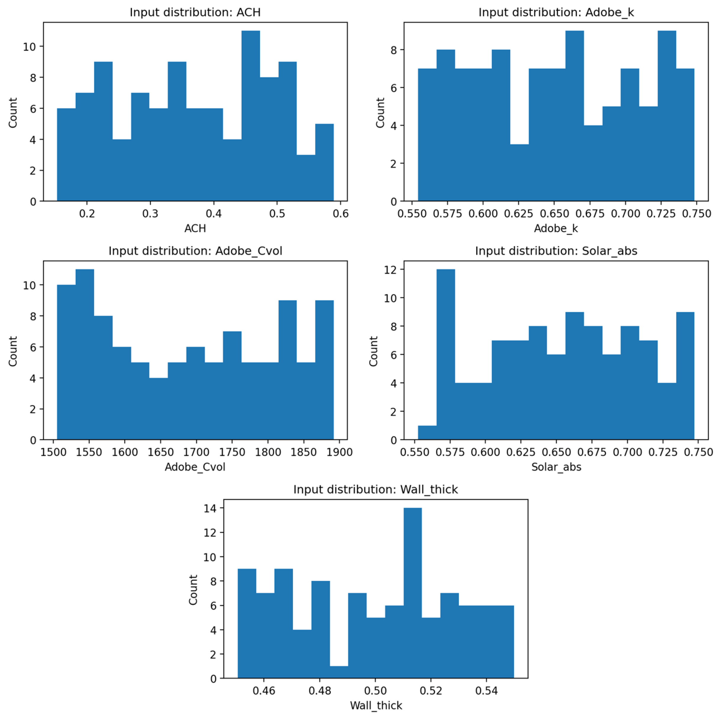
The parameters were sampled from uniform distributions within explicit lower and upper bounds derived from literature and field constraints, as reported in Table 6.

Each parameter set was evaluated in IDA ICE using its parametric run functionality. This tool automates repeated simulations by systematically varying the input values according to the defined distributions. After the runs were completed, the ensemble of results was analysed statistically. Percentile ranges (e.g., 5th–95th percentile envelopes) were derived to illustrate the spread of possible outcomes, and the mean trajectory was compared with the baseline case.

4. Results

4.1. Indoor Environmental Monitoring Results

The August monitoring campaign highlighted the extreme thermal stress the dwelling experienced during the summer. Outdoor air temperatures during this period averaged 40.2 °C, ranging from 32.7 °C to 47.7 °C. Indoor conditions were somewhat moderated by the building envelope, with an average of 38.1 °C, a maximum of 40.3 °C, and a minimum of 35.9 °C. While these results suggest that the massive adobe walls attenuated the peak outdoor extremes, indoor temperatures still remained above comfort thresholds for prolonged periods. Mean relative humidity was low, averaging 22.9% outdoors and 20.0% indoors, reflecting the arid climatic context.

In September, the monitoring captured milder climatic conditions. Outdoor temperatures averaged 36.1 °C, while indoor temperatures were slightly higher at 36.3 °C. Maximum values indoors and outdoors were nearly identical (43.5 °C and 43.4 °C, respectively), although the indoor minimum of 34.4 °C remained higher than the outdoor minimum of 30.5 °C, again reflecting the envelope’s buffering effect. Relative humidity values were slightly higher than in August, averaging 24.7% outdoors and 20.8% indoors. These differences highlight that the building moderates diurnal extremes but maintains persistently elevated indoor temperatures during the summer months.

To capture the dynamic thermal response of the dwelling beyond minimum/maximum/average values, the monitored time series were additionally analysed in terms of the hourly temperature difference ΔT = T_out − T_in and its day–night behaviour and a semi-quantitative time-lag between outdoor and indoor air temperature peaks. Using hourly means over the continuous monitoring windows, ΔT was predominantly positive during daytime, indicating indoor cooling relative to outdoors (e.g., in the August window, ΔT averaged ≈4.7 °C during 08:00–18:00, with peaks up to ≈8.7 °C), while nighttime ΔT was much smaller (≈0.2 °C) and occasionally inverted, reflecting the damping effect of the earthen envelope. The indoor diurnal temperature swing was markedly attenuated compared to outdoors (indoor range ≈ 3–4 °C versus outdoor ≈ 12–15 °C across the two campaigns), and cross-correlation of the hourly profiles indicates an indoor peak delay of ~1–3 h, consistent with thermal inertia. For relative humidity, the discussion was expanded to include not only mean values but also minimum and maximum values: indoor RH ranged approximately 17–26% in the August window and 14–34% in the September window (hourly), compared to outdoor ranges of about 17–35% and 15–45%, respectively, with indoor RH exceeding 30% only briefly during the September campaign (≈7% of hours). These additional indicators provide a clearer basis for interpreting the building’s buffering capacity and its differentiated daytime/nighttime behaviour.

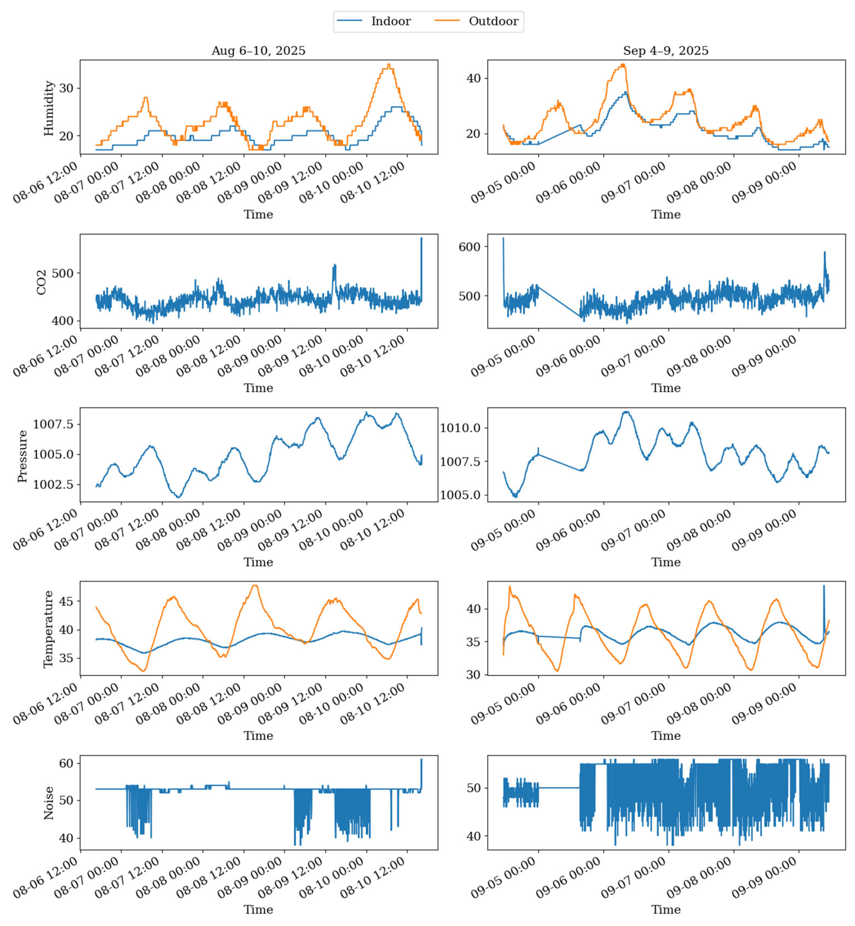
In addition to thermal and humidity measurements, the monitoring campaign also recorded carbon dioxide (CO₂) concentration, pressure, and noise levels (Figure 10). CO₂ remained stable around 400–500 ppm, consistent with unoccupied or sparsely occupied conditions, while pressure showed expected diurnal fluctuations linked to outdoor weather patterns. Noise data showed occasional peaks from external sources, but the dwelling itself provided limited acoustic buffering. Together, these additional variables confirm that the building envelope primarily affects thermal and moisture dynamics, while indoor air quality and noise levels are more directly influenced by external boundary conditions.

Table 7. Summary of indoor and outdoor thermal conditions and relative humidity statistics (mean, minimum, and maximum) for the August and September 2025 monitoring campaigns.

Month	Location	Mean Temp (°C)	Max Temp (°C)	Min Temp (°C)	Mean Humidity (%)	Min Humidity (%)	Max Humidity (%)
August	Indoor	38.12	40.3	35.9	20.0	17	26
August	Outdoor	40.22	47.7	32.7	22.86	17	35
September	Indoor	36.27	43.5	34.4	20.82	14	34
September	Outdoor	36.07	43.4	30.5	24.69	15	45

provides a summary of indoor and outdoor mean, maximum, and minimum temperatures, together with mean, minimum, and maximum relative humidity values for both campaigns. This combined dataset serves as the basis for subsequent affine adjustment of the simulated temperature series and for evaluating building-envelope performance.

To complement the descriptive monitoring results, additional short-window passive performance indicators were derived from the monitored data for each campaign window. These include estimated time lag, decrement factor, damping behaviour, exceedance hours above 30 °C and 35 °C, and degree-hours above 30 °C (

Table 8. Short-window passive performance indicators derived from the monitored indoor and outdoor temperature data for the August and September 2025 campaigns. The exceedance-hour and degree-hour columns refer to indoor air temperature thresholds.

Period	Time Lag Estimate, Hours	Decrement Factor Estimated	Indoor Hours Above 30 °C	Indoor Hours Above 35 °C	Indoor Degree-Hours Above 30 °C
6–10 August 2025	3	0.217	97	97	788.08
4–9 September 2025	1	0.308	107	92	670.57

). Although based on short monitoring periods, these indicators are sufficiently robust for limited-duration analysis and provide a useful basis for comparing the dwelling’s passive thermal response across the two campaigns, without extending the interpretation to seasonal generalization [51,52].

4.2. Raw Physics-Based Model Comparison Against Monitored Indoor Temperature

Measured indoor air temperatures from 6–10 August 2025, were compared with the IDA ICE baseline simulation. Hourly averages of the sensor data were aligned with the simulation output.

The model agreement was quantified using the root-mean-square error (RMSE), computed from the hourly measured indoor temperatures and the corresponding simulated indoor temperatures at matched time steps.

$$RMSE=\sqrt{{\displaystyle \frac{1}{N}}\sum _{i=1}^N{\left(T_{m,i}−T_{s,i}\right)}^2}$$

RMSE represents the typical magnitude of the temperature error in °C during the evaluated comparison window. Mean bias error (MBE) and the coefficient of variation of RMSE (CVRMSE) were also computed as

$$MBE={\displaystyle \frac{1}{N}}\sum _{i=1}^N\left(T_{s,i}-T_{m,i}\right),CVRMSE={\displaystyle \frac{RMSE}{\overline{T_m}}}\times 100\%$$

where $\overline{T_m}$ is the mean of the measured indoor temperature over the same window.

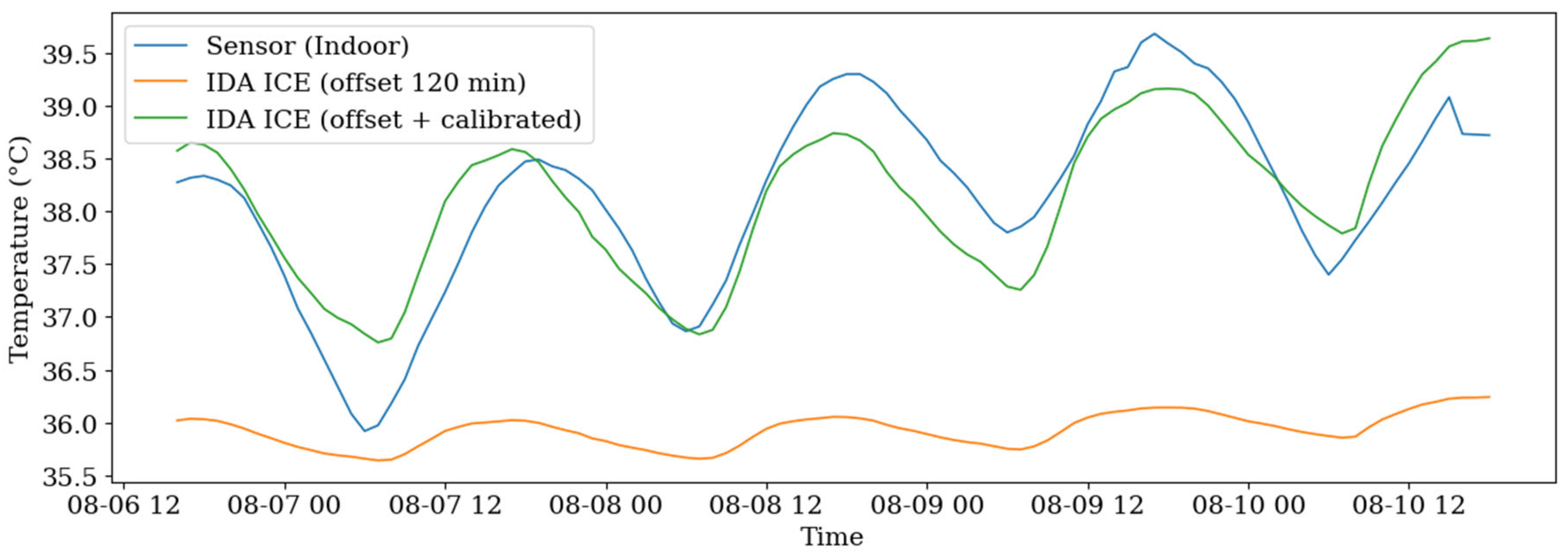
A systematic offset search identified a 120 min lag between the model and the measurements, likely due to a mismatch between the logger reference and the thermal response. Although applying this shift improved the correlation (r from 0.71 to 0.84), the model still underestimated both the mean level and the amplitude. The raw physics-based model output, with and without time-offset alignment, therefore serves as the primary basis for interpreting model performance during the monitored periods.

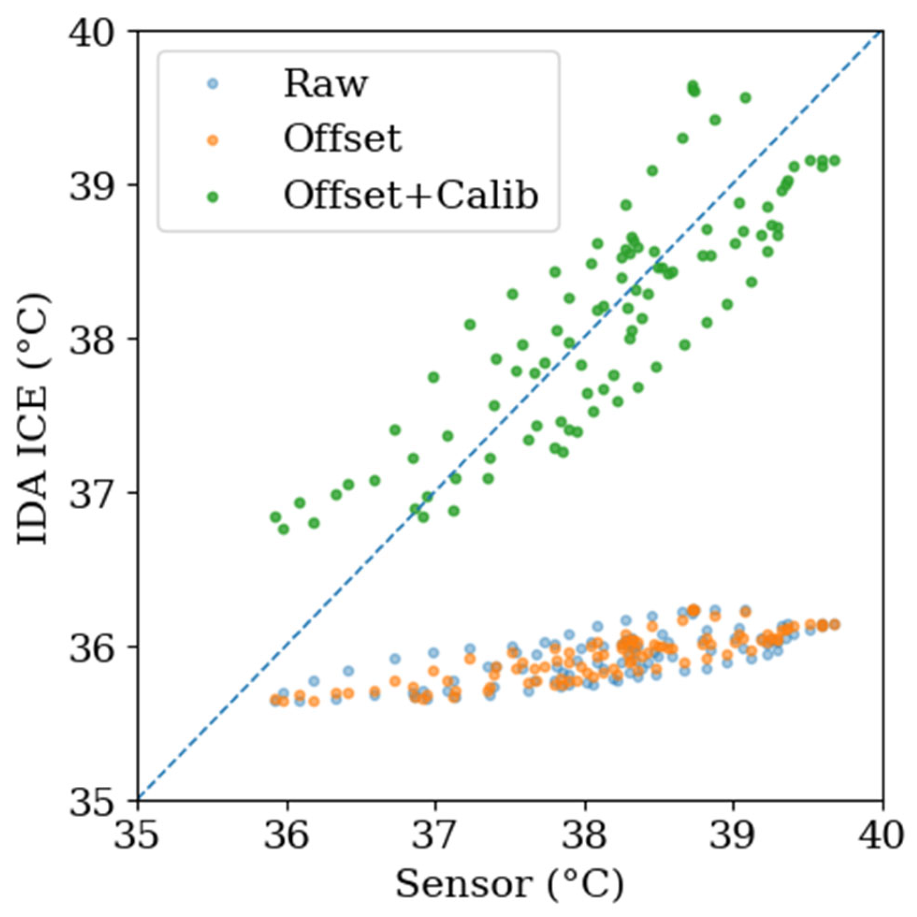
To explore any remaining systematic offset, a simple affine mapping was computed for the August window only as a diagnostic post-processing step of the simulated indoor temperature series. This mapping is not a physical calibration of model parameters and is not used here as evidence of the model’s transferable accuracy. Rather, it is reported only to illustrate the magnitude of short-window linear bias that may arise from residual effects such as sensor bias, unmodelled micro-ventilation events, or local radiative influences. Because this August-derived affine mapping does not transfer to the independent September window, increasing RMSE and introducing a positive bias, it is interpreted strictly as a non-transferable diagnostic bias correction rather than as a robust basis for model evaluation.

To illustrate the magnitude of residual systematic bias within the August fitting window, a simple affine adjustment was applied of the form:

$${\mathrm{T}}_{\text{bias-adjusted}}=\mathrm{a}+\mathrm{b}\hspace{0.17em}{\mathrm{T}}_{\mathrm{IDA}}$$

With fitted coefficients, this adjustment substantially improved agreement, reducing RMSE from 2.34 °C (raw) to 0.47 °C and eliminating the mean bias.

The affine mapping is presented solely as a post-processing bias correction to illustrate systematic offsets and is not intended as a physical adjustment of building parameters; such adjustments should instead target infiltration, solar gains, and envelope properties [53,54].

To assess whether the raw physics-based model remained plausible beyond the August monitoring window, an independent comparison was carried out using the September monitoring period. The August window was used only to identify the diagnostic affine mapping, whereas the September window served as an out-of-sample test of transferability without re-fitting. This separation was used to verify whether the August-derived post-processing correction remained representative under different boundary conditions and to reduce the risk of overfitting to a single short window. The hourly indoor air temperature datasets used for this comparison are summarized in

Table 9. Hourly measured indoor air temperature used for diagnostic affine-bias identification and independent out-of-sample comparison.

Monitoring Period	Use in Study	N (Hourly)	Mean (°C)	Min (°C)	Max (°C)
6–10 August 2025	Diagnostic bias-identification window	97	38.12	35.92	39.68
4–9 September 2025	Independent out-of-sample raw-model comparison	107	36.27	34.54	37.90

: 6–10 August 2025 (97 hourly values; mean 38.12 °C; min 35.92 °C; max 39.68 °C) and 4–9 September 2025 (107 hourly values; mean 36.27 °C; min 34.54 °C; max 37.90 °C).

The affine adjustment presented in this study was performed only on indoor air temperature, because temperature was the primary comparison variable for aligning the energy balance of the single-zone model with the short monitoring windows available. RH-related outputs are treated as exploratory sensitivity indicators, and the associated assumptions are summarized in Section 7.

To examine whether the affine adjustment derived from the August monitoring window is suitable for use outside the August adjustment window, we conducted an out-of-sample evaluation using the independent September monitoring campaign. A strict separation between adjustment and evaluation was maintained. The time offset and the affine mapping were identified using the 6–10 August 2025 dataset only, and were then applied unchanged to the 4–9 September 2025 simulation results without any re-fitting. The agreement between simulated and measured hourly indoor operative temperatures was quantified using an hourly-aligned time series.

Error was defined as $e_i=T_{\mathrm{s}\mathrm{i}\mathrm{m},i}-T_{\mathrm{m}\mathrm{e}\mathrm{a}\mathrm{s},i}$ for $i=1,\dots ,N$.

The root mean square error was computed as $\mathrm{R}\mathrm{M}\mathrm{S}\mathrm{E}=\sqrt{{\displaystyle \frac{1}{N}}{\sum }_{i=1}^N{e}_i^2}$, the mean bias error as $\mathrm{M}\mathrm{B}\mathrm{E}={\displaystyle \frac{1}{N}}{\sum }_{i=1}^N{e}_i$, and the coefficient of variation of RMSE as $\mathrm{C}\mathrm{V}\mathrm{R}\mathrm{M}\mathrm{S}\mathrm{E}={\displaystyle \frac{\mathrm{R}\mathrm{M}\mathrm{S}\mathrm{E}}{{\overline{T}}_{\mathrm{m}\mathrm{e}\mathrm{a}\mathrm{s}}}}\times 100\%$, where ${\overline{T}}_{\mathrm{m}\mathrm{e}\mathrm{a}\mathrm{s}}$ is the mean measured temperature over the same evaluation window (

Table 10. Raw physics-based, time-offset, and diagnostic affine-bias comparison results for hourly indoor operative temperature, with September used as an independent out-of-sample test. Time offset and affine coefficients were identified only for 6–10 August 2025, and applied unchanged to the independent 4–9 September 2025, monitoring period.

Period	N (Hours)	Output	RMSE (°C)	MBE (°C)	CVRMSE (Percent)
6–10 August 2025	97	Raw simulation	2.34	−2.20	6.13
6–10 August 2025	97	Time-offset only	2.33	−2.20	6.12
6–10 August 2025	97	Time-offset plus August affine	0.46	0.00	1.20
4–9 September 2025	107	Raw simulation	1.02	−0.45	2.82
4–9 September 2025	107	Time-offset only	1.00	−0.43	2.75
4–9 September 2025	107	Time-offset plus August affine	2.12	1.42	5.84

).

Table 10 presents the direct comparison between monitored indoor operative temperature and the corresponding IDA ICE output under the free-running configuration, using only the physically defined envelope and boundary conditions described in Section 3.3. The agreement is already strong during the September monitoring window, with an RMSE of 1.02 °C, indicating that the model provides a physically consistent representation of the dwelling’s dominant passive thermal dynamics within the monitored periods, including diurnal swing, time lag, and damping, without empirical tuning. We therefore interpret the raw comparison as preliminary evidence that the model provides plausible representation of the main passive thermal behaviour of the monitored dwelling over the available windows, supporting comparative behavioural interpretation rather than rigorous absolute accuracy claims. Accordingly, the monitored dataset supports relative interpretation of model behaviour within the monitored periods rather than validation of model accuracy under broader conditions.

The comparison between measured and simulated indoor temperature indicates that the raw physics-based model is consistent with the dominant passive thermal dynamics observed in the monitored data of the dwelling, including diurnal variation, time lag, and damping effects. While a diagnostic affine adjustment reduces error within the August window, its lack of transferability to the independent September dataset confirms that it reflects short-window residual effects (e.g., sensor bias or unmodelled micro-scale processes) rather than physically meaningful calibration. Therefore, the interpretation of model performance relies primarily on the raw physics-based results, with the affine adjustment used only to illustrate the magnitude of systematic offsets within constrained monitoring conditions.

Applying the same time offset identified in August yields only a small additional improvement in September (RMSE 1.00 °C). The August-derived affine adjustment is therefore retained only as a short-window diagnostic post-processing step and not as a transferable correction across periods; the out-of-sample September results support reliance on the raw physics-based model for interpretation.

A direct monitored–simulated comparison proved particularly challenging with such a dataset. The monitoring campaign was short and subject to gaps and sensor inconsistencies, requiring careful preprocessing. Aligning time references, correcting logger drift, and accounting for thermal response delays all added complexity. Moreover, only one primary indoor sensor location was used for the quantitative comparison; the second indoor module served only as a qualitative spatial cross-check in an adjacent space and was not used for averaging or direct model comparison. This limits the ability to assess indoor spatial variability rigorously or to compare relative humidity and air-quality-related outputs across multiple indoor positions.

Given the short monitoring duration, data gaps, preprocessing challenges, and the use of only one primary indoor sensor for quantitative comparison, affine adjustment was performed using the August monitoring window, while the September window was used as an out-of-sample check to assess robustness without re-fitting. This provides only a narrow feasibility check of short-window model comparison under constrained field conditions. Expanding the monitoring period, increasing the number of sensors, and automating parts of the affine-adjustment workflow will be important next steps. The next phase should extend the monitored period to at least one month and broaden the comparison beyond temperature to include relative humidity and ventilation-related indicators, strengthening the robustness of the digital-twin workflow.

The comparison between monitored and simulated indoor temperatures is illustrated through a time-series overlay (Figure 11) and a scatter plot against the 1:1 reference line (Figure 12). Owing to the limited duration and coverage of the monitoring campaign, the quantitative comparison was restricted to indoor temperature, while other variables, such as relative humidity and CO₂, were not included due to higher uncertainty and data limitations.

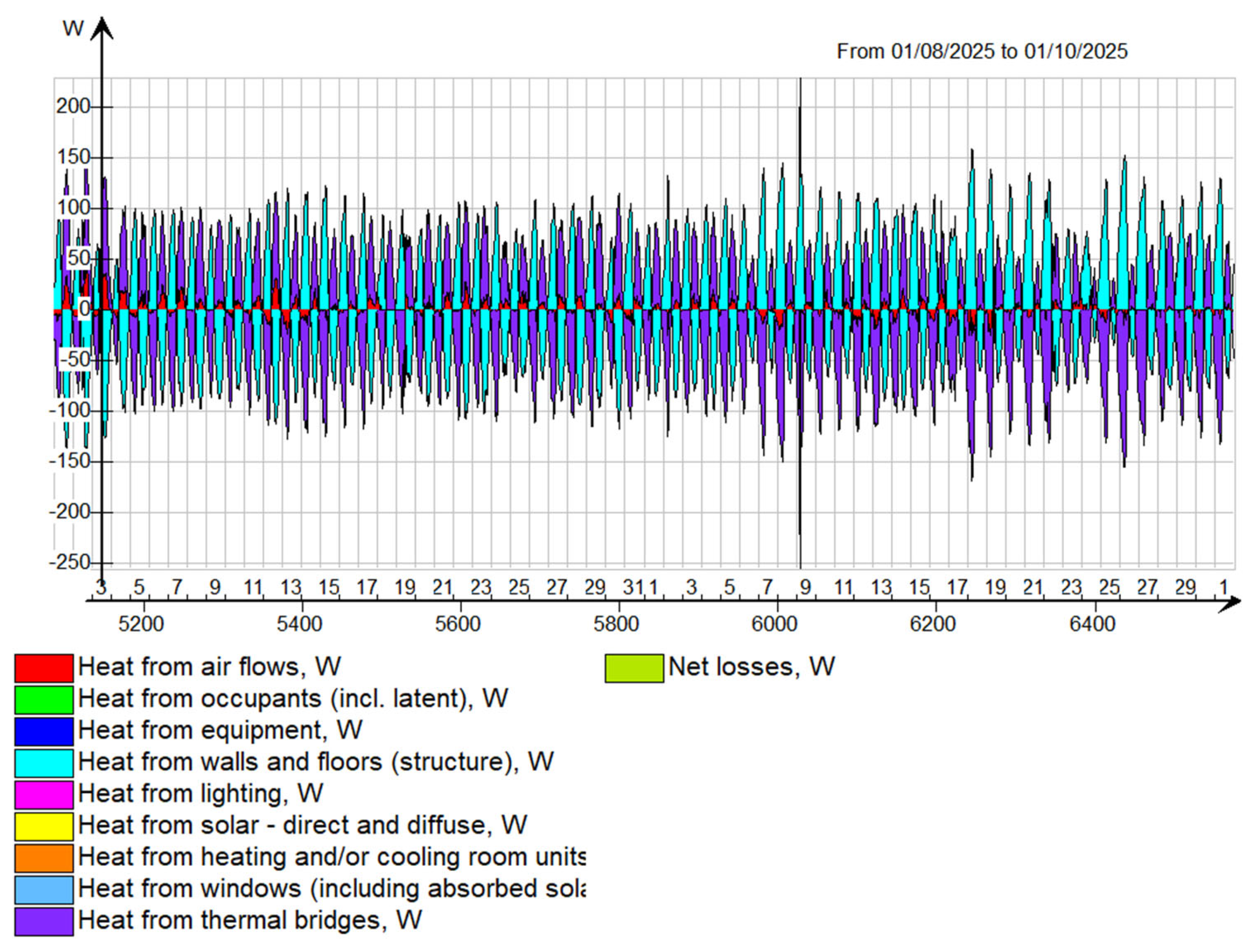
Figure 13 presents the hourly heat balance of the simulated dwelling from 1 August to 1 October 2025, illustrating the temporal interaction between internal and external heat gains and losses that govern indoor thermal conditions. This indicates that solar gains dominate daytime heat input, while transmission losses and infiltration govern nocturnal heat dissipation, highlighting the asymmetric role of passive processes across the diurnal cycle.

The dominant positive contributions arise from solar radiation and direct solar gains on the structure. On the loss side, thermal transmission through walls, windows, and thermal bridges, as well as infiltration airflows, account for significant negative values, driving the oscillating heat balance observed across the period. The daily cycles of solar input are clearly reflected in the amplitude of fluctuations, with peaks during daytime and losses at night. Net heat losses remain evident throughout, underscoring the dwelling’s passive nature under free-running conditions and the absence of active heating or cooling systems. This balance highlights the critical role of solar gains and infiltration in shaping the building’s thermal behavior during summer and early autumn. Consequently, temperature is treated as the primary variable for model–measurement comparison, while RH is analysed separately as a sensitivity-driven indicator due to higher uncertainty.

4.3. Uncertainty Analysis Results from Monte Carlo Simulations

Within this exploratory framework, the Monte Carlo analysis is used to rank the relative influence of uncertain inputs on MaxRH within the assumed hygrothermal model structure. Relative humidity (RH) is analysed here as a sensitivity-driven indicator to explore moisture-related risks under uncertainty, rather than as a validated predictive output, due to the absence of extended monitoring and the additional uncertainties associated with moisture processes, where the corresponding assumptions and limitations are discussed in Section 7.

Figure 14 presents the distributions of input variables used in the Monte Carlo experiment. Uniform sampling was adopted to ensure an even exploration of the uncertainty space. The figure summarizes the sampling structure and supports the interpretation of subsequent results.

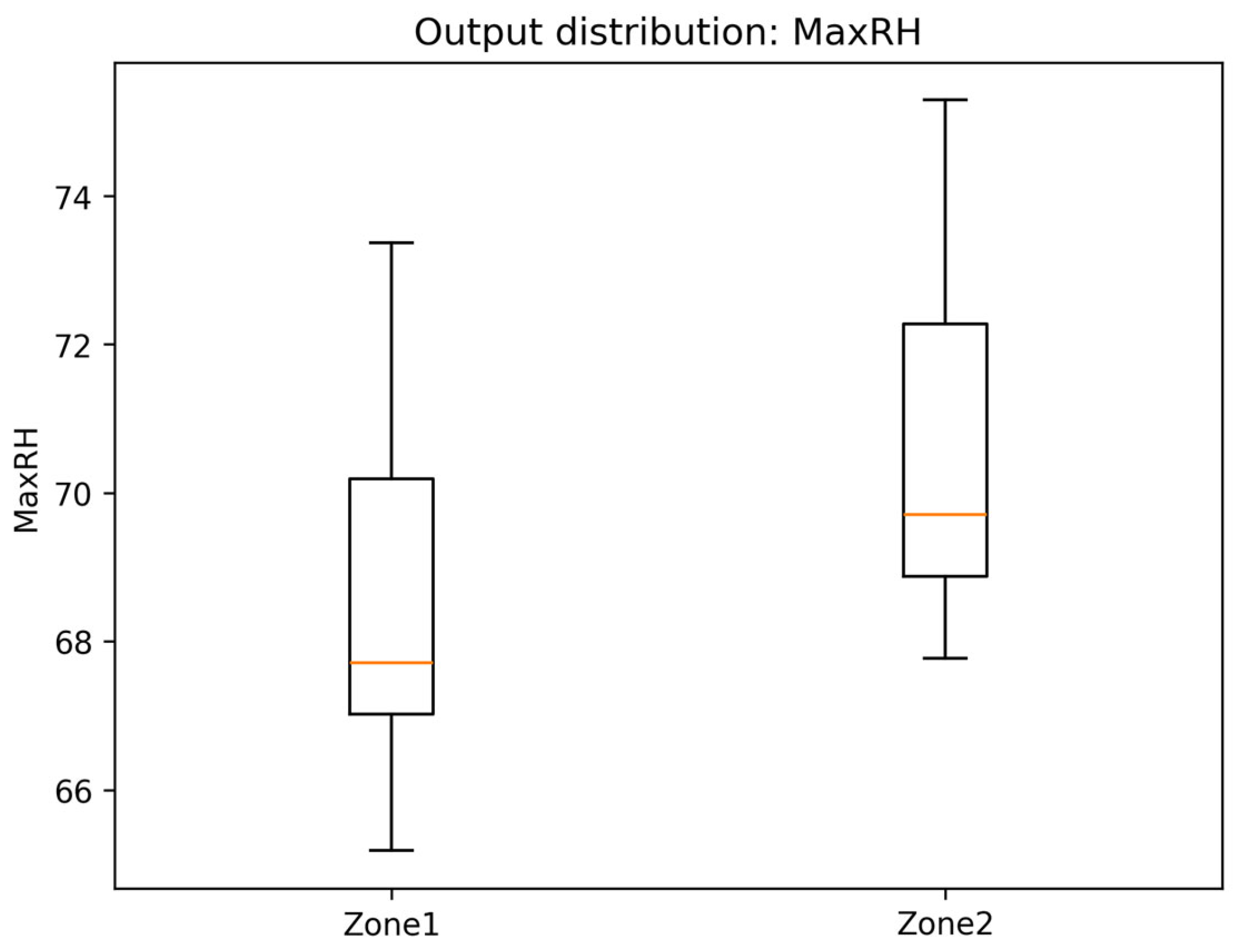
As shown in Figure 15, the Monte Carlo results indicate that infiltration exerts the strongest influence on MaxRH within the tested parameter ranges, whereas wall thickness, adobe thermal conductivity, adobe volumetric heat capacity, and surface solar absorptance have comparatively smaller effects. These outputs should be interpreted as sensitivity-ranking results within the assumed model structure, not as probabilistic forecasts of future indoor humidity conditions. The maximum relative humidity (MaxRH) consistently reaches higher levels in the upper zone (second floor) compared to the lower one (first floor), despite identical boundary conditions and input parameter ranges, which suggests that vertical stratification and envelope exposure contribute to higher peak moisture levels upstairs, while the lower zone remains slightly more stable. The boxplots also show that the variability in MaxRH is broader in the upper zone, indicating that uncertainty in inputs such as infiltration and envelope properties propagates more strongly into the upper thermal environment. This difference underscores the importance of accounting for intra-building variation when evaluating comfort and moisture risks.

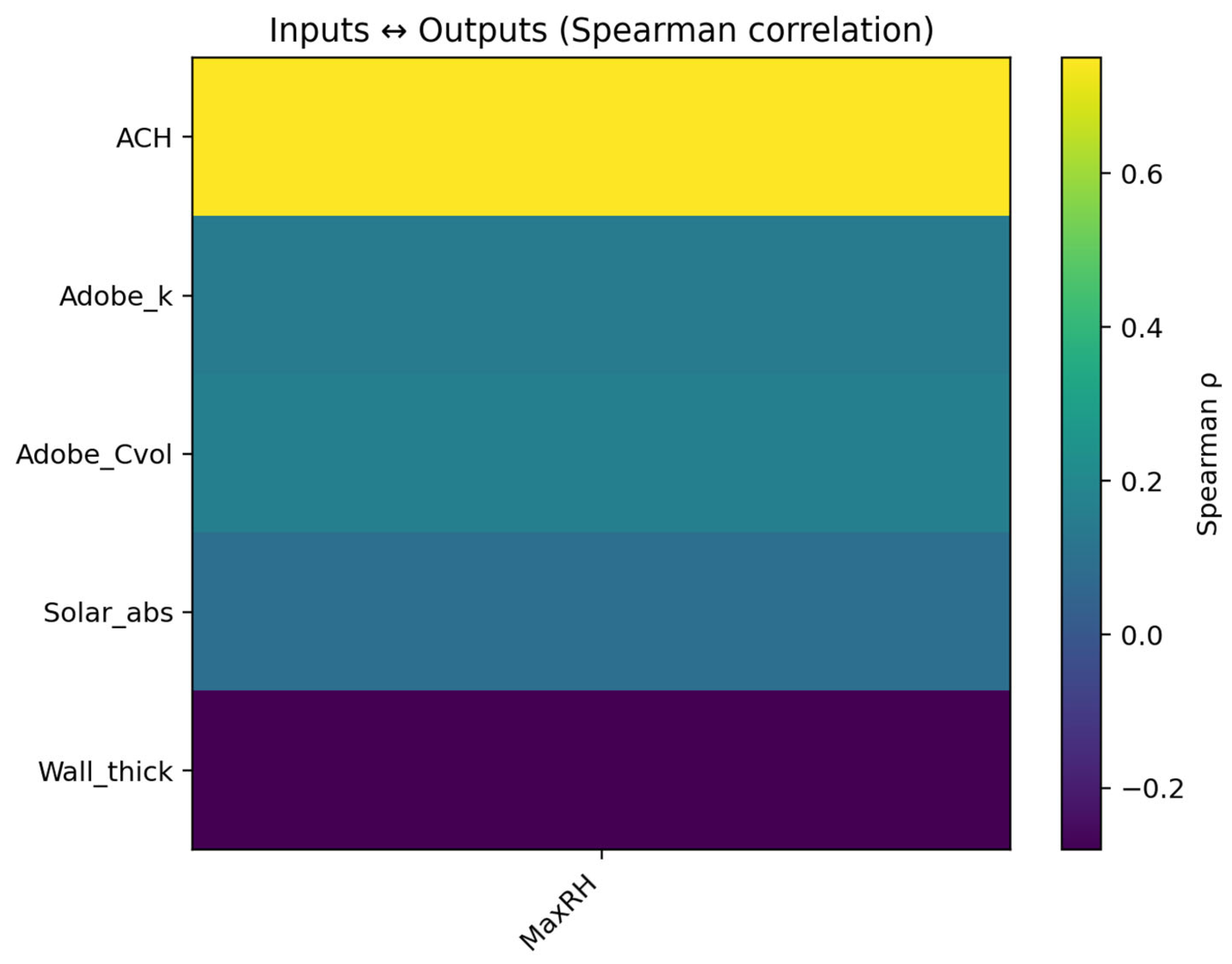
Figure 16 presents the Spearman rank correlations between the five input parameters and MaxRH. The results indicate that infiltration rate (air changes per hour, ACH) emerges as the dominant parameter within the assumed model structure and tested ranges within the explored sensitivity space, with a strong, monotonic positive association with MaxRH. In other words, as infiltration increases, so too does indoor peak humidity, reflecting the greater exchange of moisture-laden outdoor air with the indoor environment. By contrast, adobe thermal conductivity, adobe volumetric heat capacity, and surface solar absorptance show weak or negligible correlations, suggesting they play only a minor role in shaping peak humidity conditions within the investigated ranges. Wall thickness shows a weak negative correlation, consistent with the buffering effect of higher thermal mass, though its magnitude is modest compared to that of infiltration.

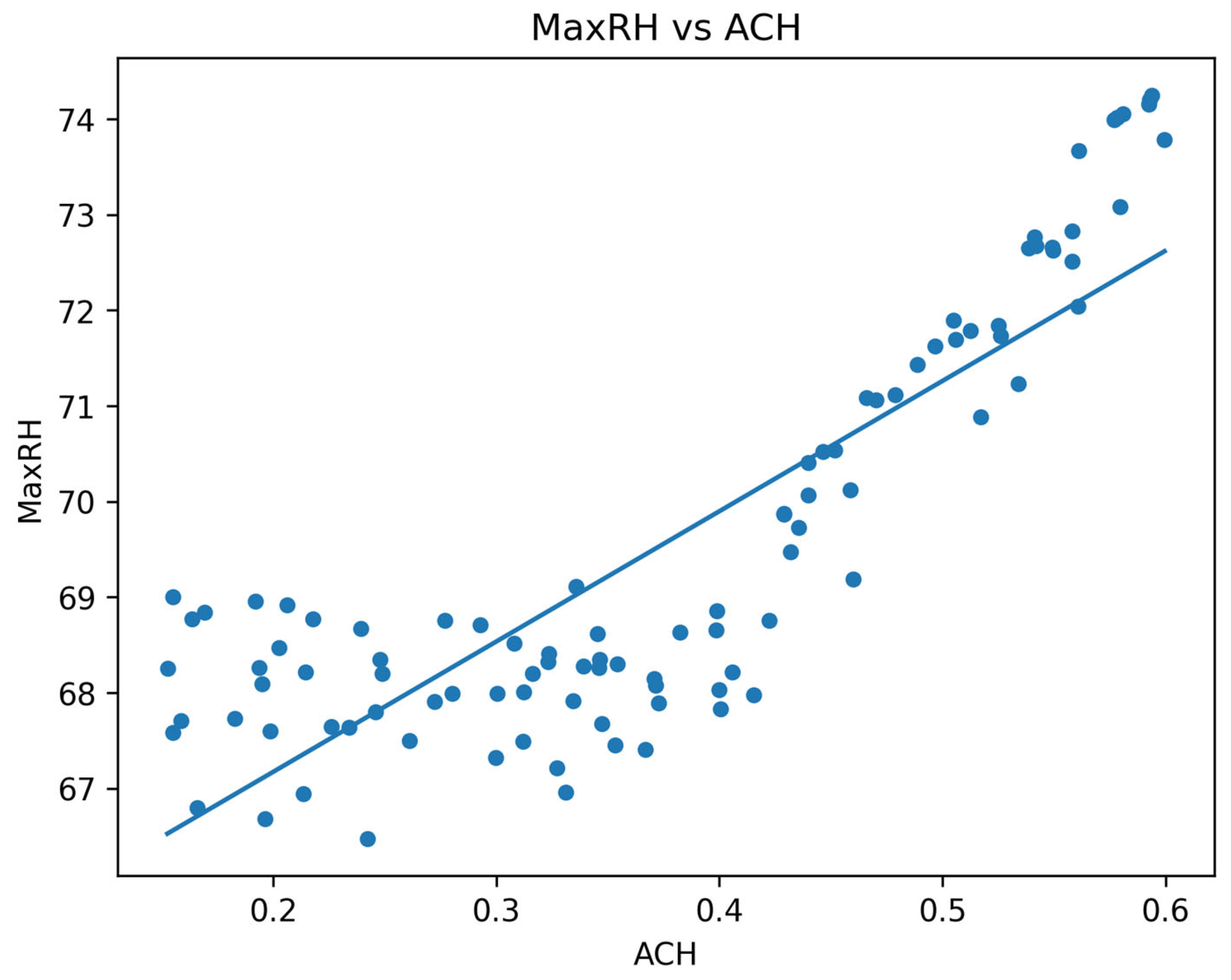
The strong role of infiltration is further illustrated by the direct bivariate relationship (Figure 17). The scatter of MaxRH against ACH shows a clear upward trend, with values of MaxRH increasing from approximately 67% at the lower infiltration bound (0.15 h⁻¹) to over 74% at the upper bound (0.60 h⁻¹) within the explored parameter space. The fitted regression line confirms the monotonic nature of this relationship, with limited scatter around the trend. This pattern supports the interpretation that infiltration is the most influential tested parameter for RH-related outcomes in the present exploratory analysis, rather than a probabilistic prediction of future indoor humidity levels. It also suggests that infiltration is practically relevant to the indoor climate of the monitored heritage dwelling within the uncertainty ranges examined.

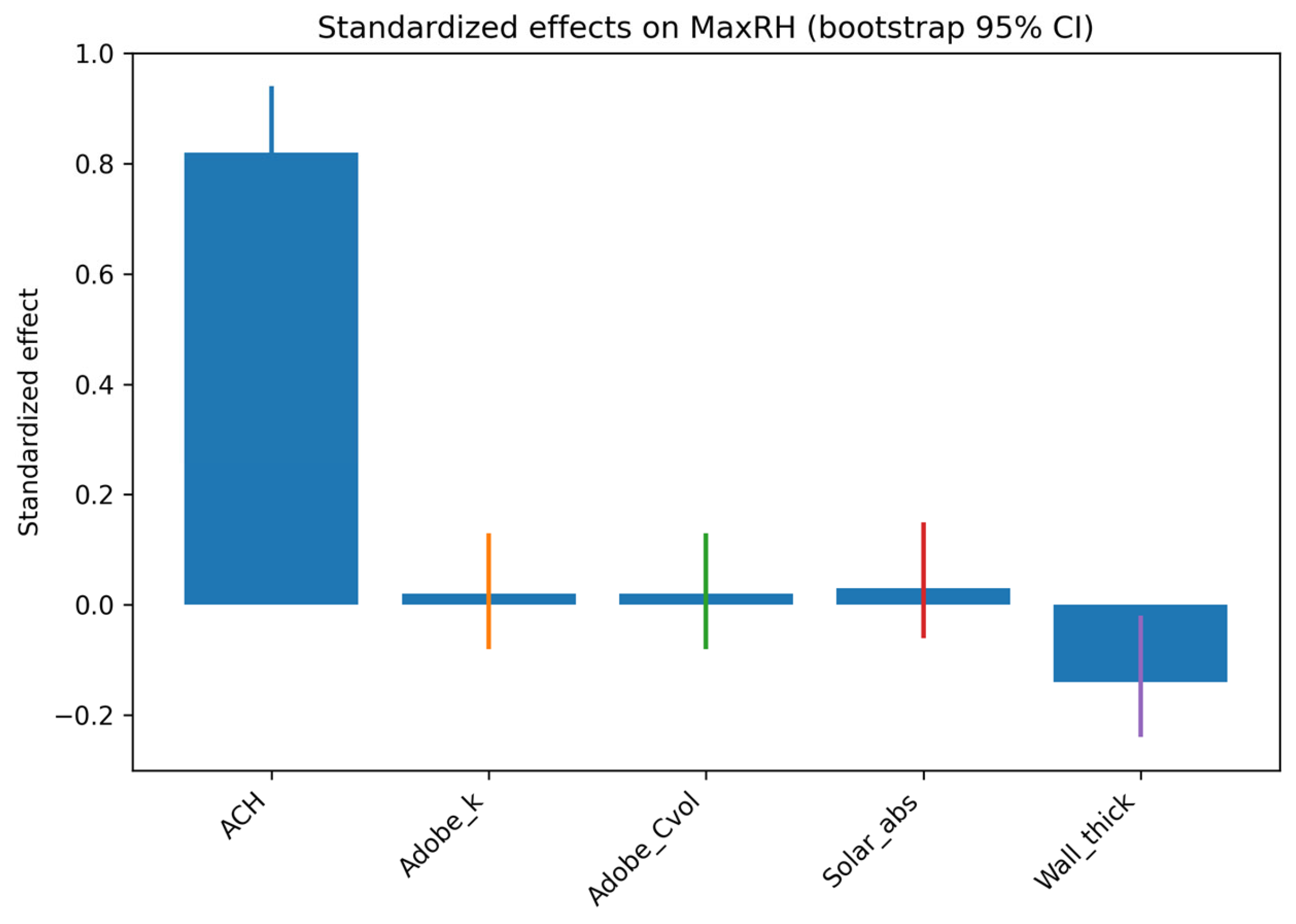
To quantify the relative contributions of each input, standardized regression analysis with bootstrap confidence intervals was performed (Figure 18). Again, the results reinforce the dominance of infiltration: ACH shows a large positive standardized effect, significantly greater than zero, supporting its interpretation as the primary tested driver of MaxRH variability within the present sensitivity framework. Wall thickness exerts a small but consistent negative effect, supporting the idea that thicker adobe walls moderate indoor humidity extremes through their combined thermal and moisture capacity. In contrast, adobe thermal conductivity (Adobe_k), adobe volumetric heat capacity (Adobe_Cvol), and surface solar absorptance (Solar_abs) all show effects close to zero, with confidence intervals overlapping the baseline, meaning they do not contribute meaningfully to the variance in MaxRH within the explored ranges. These findings should be interpreted strictly within the assumed model structure and parameter ranges, and do not constitute validated predictions of indoor moisture behaviour.

5. Discussion

The results provide a preliminary understanding of the thermal behaviour of the monitored earthen dwelling during the two summer monitoring windows. Within these monitored periods, the massive mud-brick walls attenuated outdoor fluctuations, delayed indoor peaks, and produced measurable damping of diurnal extremes. However, these findings are representative only of the monitored August and September 2025 periods and should not be generalized to seasonal or annual performance. At the same time, the absence of effective ventilation and shading mechanisms in the studied dwelling resulted in sustained indoor temperatures well above comfort thresholds. This indicates that thermal inertia, while important, was not sufficient on its own to ensure indoor thermal adequacy under the extreme summer conditions observed in central Arabia.

The integration of digital-twin modelling and field monitoring adds an important interpretive layer to the empirical findings. In particular, the combined monitoring–simulation approach demonstrates that even under constrained field conditions, it is possible to identify dominant passive mechanisms and assess model plausibility without relying on full calibration, thereby supporting feasibility-oriented applications in heritage contexts where high-resolution data are difficult to obtain. Although the August affine adjustment reduced error within the same short fitting window, the independent September comparison showed that this post-processing correction was not transferable and could increase bias, reinforcing the importance of relying primarily on the raw physics-based model for interpretation.

The raw physics-based September result is therefore treated as the more reliable basis for interpretation. By contrast, the August affine correction functioned only as a short-window diagnostic adjustment and was not transferable to the independent September period. Together with the exploratory Monte Carlo results, which identify infiltration as the dominant tested driver of RH-related sensitivity, these findings indicate that future work should prioritize longer monitoring periods, better characterization of air-exchange pathways, and broader seasonal assessment rather than short-window bias correction alone. In this respect, the study directly addresses the previously identified gap in coupled monitoring–simulation evidence for Najdi earthen dwellings by providing a first empirical–computational dataset and demonstrating a feasible workflow under real heritage-site constraints.

An important implication of these findings is that thermal buffering should not be equated with thermal adequacy in abandoned or poorly ventilated earthen dwellings during present-day summer extremes. In the monitored case, the adobe envelope delayed and damped outdoor peaks, but this passive moderation remained insufficient because stored heat was not effectively purged through night ventilation or controlled air exchange. For the monitored dwelling and the short summer periods analysed here, thermal mass alone was therefore insufficient to maintain acceptable indoor conditions, and ventilation pathways and envelope permeability emerged as important factors for further investigation. Broader conclusions for Najdi earthen dwellings will require longer multi-season monitoring and additional case studies.

This distinction is particularly important for conservation practice, where reliance on thermal mass as a primary passive strategy may lead to overestimation of performance under current climatic extremes. The results suggest that ventilation pathways and air-exchange mechanisms are equally critical components of thermal resilience in earthen heritage buildings.

From a conservation perspective, the study suggests that rehabilitation efforts should combine passive ventilation strategies, such as reactivated courtyards, wind catchers, or operable openings, with selective mechanical support when comfort thresholds are consistently exceeded. These measures can be designed to respect the authenticity of Najdi earthen fabric while ensuring resilience under future climatic extremes. The integration of empirical monitoring with digital-twin simulation provides a preliminary workflow for feasibility-oriented assessment under constrained field conditions. At this stage, the workflow should be understood as a pilot methodological approach that may inform future studies, rather than as a basis for direct generalization across similar settlements. This distinction is particularly relevant for current heritage rehabilitation policies in Saudi Arabia, where passive performance is often assumed rather than empirically verified.

6. Conclusions

This study presents a pilot methodological and feasibility investigation rather than a validated digital-twin study. The model reproduces key passive thermal behaviours observed in the monitored periods, including attenuation of diurnal peaks and short time-lag effects; however, the limited duration and resolution of the dataset do not support full validation or predictive application beyond these specific conditions.

Based on two short monitoring campaigns conducted in August and September 2025, the results indicate that during the monitored periods, the earthen envelope moderated diurnal outdoor temperature fluctuations but, on its own, did not ensure indoor comfort during peak summer conditions. The monitored–simulated comparison further suggests that the simplified physics-based model can reproduce part of the observed passive thermal behaviour over short periods; however, the non-transferability of the August affine correction confirms that the present dataset is insufficient for full digital-twin validation or for generalized performance claims. These findings are therefore representative only of the monitored periods and should not be interpreted as evidence of seasonal or year-round performance.

The main contribution of the study is therefore methodological. Specifically, the study advances current knowledge by demonstrating a field-constrained digital-twin workflow for earthen heritage buildings that explicitly integrates short-window monitoring, uncertainty-aware simulation, and non-transferable bias diagnostics, a combination that to our knowledge, no prior study has combined short-window monitoring, bias-diagnostic evaluation, and uncertainty-aware simulation for Najdi earthen dwellings.

The paper documents a feasible workflow linking short-term monitoring, geometry reconstruction, simplified IDA ICE modelling, and exploratory uncertainty analysis under difficult heritage-site conditions. More importantly, the study highlights several practical lessons from constrained monitoring in deteriorated heritage buildings, including the difficulty of maintaining continuous records, the limits of consumer-grade instrumentation, the need for careful time alignment and data preprocessing, and the importance of distinguishing comparative behavioural interpretation from rigorous absolute validation. Within the analysed period, the exploratory Monte Carlo analysis indicates that infiltration is the most influential parameter affecting RH-related sensitivity within the assumed model structure and should therefore be prioritized in future investigations, restoration, and adaptive reuse strategies.

From a practical standpoint, these findings support the prioritization of ventilation-focused interventions in conservation and adaptive reuse strategies for earthen heritage buildings in hot–arid climates, particularly in partially abandoned structures where uncontrolled air exchange governs indoor environmental conditions. More broadly, the study should be read as a preliminary framework for longer-term monitoring and future seasonal assessment, rather than as a basis for direct transferability to other dwellings or broader climatic generalization. Longer multi-season campaigns, reference-supported instrumentation, and broader comparison targets will be required before stronger conclusions about model robustness, transferability, and predictive performance can be drawn.

7. Limitations and Future Works

Despite these contributions, the study is subject to several limitations. Given the constrained monitoring duration and the limited continuous record available, the present study should be interpreted as a pilot feasibility assessment of a digital twin setup under challenging field conditions rather than a full, seasonally representative evaluation.

As a result, model agreement achieved within the available monitoring windows primarily supports the plausibility of the adopted boundary conditions and parameter ranges for the as-found state of the dwelling and the feasibility of using the workflow for comparative analyses within similar short periods. However, generalization across seasons, longer-term degradation dynamics, and moisture-driven processes remains provisional until extended multi-season (ideally annual) measurements and additional monitored target variables for model comparison and refinement become available. Monitoring was limited to two short summer campaigns, which constrained the ability to capture seasonal variation, occupant-driven dynamics, and long-term deterioration. The effective continuous record spans only a short period (approximately 10–11 days); therefore, the dataset cannot capture the full range of seasonal variability, episodic events, or longer-term thermal lag effects that typically govern vernacular building performance, and the generality of the derived conclusions should be interpreted cautiously. The dwelling’s abandoned state, while representative of many structures in Ushaiger, may not fully reflect performance in inhabited houses where occupancy, shading devices, and night ventilation influence indoor climate. In the simulation model, several assumptions were necessary for collapsed volumes, missing door leaves, and boundary conditions, which introduce uncertainty that the post-processing affine adjustment does not remove.

Relative humidity should be interpreted more cautiously than temperature in the present study. Although indoor RH was measured and is reported descriptively, it was not used as a primary comparison target, and the model was not formally evaluated against moisture-related state variables because of the short monitoring duration and the additional uncertainties associated with moisture sources and sinks, air exchange, the abandoned condition of the dwelling, and field measurement limitations [46,47]. In addition, key hygric material parameters, including vapour diffusion resistance factors (μ) for adobe and renders, were adopted from literature ranges rather than measured on site. For these reasons, RH-related outputs, including MaxRH, are presented as exploratory sensitivity results within the assumed model structure rather than as predictive humidity estimates. Future work should strengthen RH-specific evaluation by extending monitoring campaigns, conducting additional moisture-related material characterization, and comparing simulated and monitored humidity-related indicators.

During preprocessing, brief gaps (≤15 min) were treated as short transmission losses and were interpolated to preserve continuity for time-series analysis, whereas longer gaps (>15 min) were retained as missing values and were not interpolated to avoid introducing artificial trends. Consequently, analyses and affine adjustments of the simulated temperature series were restricted to the available continuous monitoring windows. Future work should extend monitoring to cover full annual cycles and additional dwellings in different states of preservation, creating a more robust dataset for both validation and comparative analysis. A more robust on-site power supply strategy should also be implemented to minimize outages and improve data continuity.

Coupling hygrothermal sensors with occupancy logging would enable a more detailed understanding of moisture buffering, air quality, and adaptive comfort responses. On the modelling side, integrating hygrothermal modules, knowledge graphs, and advanced optimization techniques could deepen insights into retrofit strategies and their trade-offs. Ultimately, scaling this approach across Saudi heritage settlements will enable evidence-based conservation guidelines that balance cultural authenticity with environmental performance, while also informing contemporary ecological design inspired by vernacular traditions.

References

1. Ben-Alon, L.; Rempel, A.R. Thermal Comfort and Passive Survivability in Earthen Buildings. Build. Environ. 2023, 238, 110339. [Google Scholar] [CrossRef] [Scilit]
2. Mazzetto, S. Fostering National Identity Through Sustainable Heritage Conservation: Ushaiger Village as a Model for Saudi Arabia. Heritage 2025, 8, 4. [Google Scholar] [CrossRef] [Scilit]
3. AL-Mohannadi, A.S.; Furlan, R. The Spatiality of the Vernacular Courtyard House in the Arabian Gulf Region. Heritage 2025, 8, 268. [Google Scholar] [CrossRef] [Scilit]
4. Shukla, A.; Tiwari, G.N.; Sodha, M.S. Embodied Energy Analysis of Adobe House. Renew. Energy 2009, 34, 755–761. [Google Scholar] [CrossRef] [Scilit]
5. Ben-Alon, L.; Loftness, V.; Harries, K.A.; DiPietro, G.; Hameen, E.C. Cradle to Site Life Cycle Assessment (LCA) of Natural vs Conventional Building Materials: A Case Study on Cob Earthen Material. Build. Environ. 2019, 160, 106150. [Google Scholar] [CrossRef] [Scilit]
6. Ramezannia, A.; Gocer, O.; Bashirzadeh Tabrizi, T. The Life Cycle Assessment of Stabilized Rammed Earth Reinforced with Natural Fibers in the Context of Australia. Constr. Build. Mater. 2024, 416, 135034. [Google Scholar] [CrossRef] [Scilit]
7. Dwidar, S.I.; Metwally, W.; Abbas Abdelsattar, A. Analytical Study of Heritage Residential Buildings in the Central Region of Saudi Arabia. JES J. Eng. Sci. 2020, 48, 82–93. [Google Scholar] [CrossRef] [Scilit]
8. Metwally, W.M.; Ibrahim, V.A.R. The Integration of Bio-Active Elements into Building Façades as a Sustainable Concept. Buildings 2024, 14, 3086. [Google Scholar] [CrossRef] [Scilit]
9. Moscatelli, M. Rethinking the Heritage through a Modern and Contemporary Reinterpretation of Traditional Najd Architecture, Cultural Continuity in Riyadh. Buildings 2023, 13, 1471. [Google Scholar] [CrossRef] [Scilit]
10. Dwidar, S.I. Bioclimatic Architecture for Heritage Residential Buildings in the Kingdom of Saudi Arabia. Environmental Design Approach Towards Providing Thermal Comfort in Future Buildings. JES J. Eng. Sci. 2019, 47, 868–882. [Google Scholar] [CrossRef] [Scilit]
11. Basunbul, A.I.; Braham, W.W. Climate Responsive Lessons from an Architectural and Ethnographic Study of Hijazi Traditional Dwellings in Jeddah, Saudi Arabia. Front. Built Environ. 2023, 9, 1127615. [Google Scholar] [CrossRef] [Scilit]
12. Sirror, H. Lessons Learned from the Past: Tracing Sustainable Strategies in the Architecture of Al-Ula Heritage Village. Sustainability 2024, 16, 5463. [Google Scholar] [CrossRef] [Scilit]
13. Furlan, R. Modern and Vernacular Settlements in Doha: An Urban Planning Strategy to Pursue Modernity and Consolidate Cultural Identity. Arts Soc. Sci. J. 2016, 7, 1000171. [Google Scholar]
14. Al-Oraier, F. The Thermal Analysis of Traditional Adobe Dwellings in Riyadh City, Saudi Arabia. Ph.D. Thesis, Cardiff University, Cardiff, UK, 2005. [Google Scholar]
15. Al-Hemiddi, N.A.; Megren Al-Saud, K.A. The Effect of a Ventilated Interior Courtyard on the Thermal Performance of a House in a Hot–Arid Region. Renew. Energy 2001, 24, 581–595. [Google Scholar] [CrossRef] [Scilit]
16. Jastaneyah, Z.; Kamar, H.M.; Hashmi, A.; Ghaleb, F.A.; Al Garalleh, H. The Influence of Zonal Air Supply on Thermal Comfort in a Classroom Located in a Hot and Humid Environment: A Case Study from Jeddah—Saudi Arabia. Discov. Sustain. 2024, 5, 526. [Google Scholar] [CrossRef] [Scilit]
17. Alnaim, M.M. Understanding the Traditional Saudi Built Environment: The Phenomenon of Dynamic Core Concept and Forms. World J. Eng. Technol. 2022, 10, 292–321. [Google Scholar] [CrossRef]
18. Alnaim, M.M. Traditional Najdi Settlement Architectural Elements: Harmonizing Function, Aesthetics, and Shared Socio-Cultural Meaning. J. Archit. Plan.—King Saud Univ. 2021, 33, 261–276. [Google Scholar] [CrossRef] [Scilit]
19. Alnaim, M.M. The Hierarchical Order of Spaces in Arab Traditional Towns: The Case of Najd, Saudi Arabia. World J. Eng. Technol. 2020, 8, 347–366. [Google Scholar] [CrossRef]
20. Mazzetto, S. Sustainable Heritage Preservation to Improve the Tourism Offer in Saudi Arabia. Urban Plan. 2022, 7, 195–207. [Google Scholar] [CrossRef] [Scilit]
21. Khaksar, A.; Tabadkani, A.; Mofidi Shemirani, S.M.; Hajirasouli, A.; Banihashemi, S.; Attia, S. Thermal Comfort Analysis of Earth-Sheltered Buildings: The Case of Meymand Village, Iran. Front. Archit. Res. 2022, 11, 1214–1238. [Google Scholar] [CrossRef] [Scilit]
22. Eman Sabry Abowardah, S.D. Contemporary Islamic Architecture Towards Preserving Islamic Heritage. In Proceedings of the ARCHDESIGN’ 14 on design methodologies, Istanbul, Turkey, 8–10 May 2014. [Google Scholar]
23. Ascione, F.; Bianco, N.; De Stasio, C.; Mauro, G.M.; Vanoli, G.P. Simulation-Based Model Predictive Control by the Multi-Objective Optimization of Building Energy Performance and Thermal Comfort. Energy Build. 2016, 111, 131–144. [Google Scholar] [CrossRef] [Scilit]
24. Carrobé, A.; Rincón, L.; Martorell, I. Thermal Monitoring and Simulation of Earthen Buildings. A Review. Energies 2021, 14, 2080. [Google Scholar] [CrossRef] [Scilit]
25. Idrissi Kaitouni, S.; Chahboun, R.; Bouhssine, Z.; Cakan, M.; Brigui, J.; Ahachad, M. Simulation-Based Assessment of the Climate Change Impact on Future Thermal Energy Load and Indoor Comfort of a Light-Weight Ecological Building across the Six Climates of Morocco. Therm. Sci. Eng. Prog. 2023, 45, 102137. [Google Scholar] [CrossRef] [Scilit]
26. Mazzetto, S.; Vanini, F. Urban Heritage in Saudi Arabia: Comparison and Assessment of Sustainable Reuses. Sustainability 2023, 15, 9819. [Google Scholar] [CrossRef] [Scilit]
27. Singh, M.; Fuenmayor, E.; Hinchy, E.; Qiao, Y.; Murray, N.; Devine, D. Digital Twin: Origin to Future. Appl. Syst. Innov. 2021, 4, 36. [Google Scholar] [CrossRef] [Scilit]
28. Yang, W.; Xu, J.; Lu, Z.; Yan, J.; Li, F. A Systematic Review of Indoor Thermal Environment of the Vernacular Dwelling Climate Responsiveness. J. Build. Eng. 2022, 53, 104514. [Google Scholar] [CrossRef] [Scilit]
29. Pan, Y.; Zhong, W.; Zheng, X.; Xu, H.; Zhang, T. Natural Ventilation in Vernacular Architecture: A Systematic Review of Bioclimatic Ventilation Design and Its Performance Evaluation. Build. Environ. 2024, 253, 111317. [Google Scholar] [CrossRef] [Scilit]
30. Salameh, M.; Abu-Hijleh, B.; Touqan, B. Impact of Courtyard Orientation on Thermal Performance of School Buildings’ Temperature. Urban Clim. 2024, 54, 101853. [Google Scholar] [CrossRef] [Scilit]
31. Alayed, E.; Bensaid, D.; O’Hegarty, R.; Kinnane, O. Thermal Mass Impact on Energy Consumption for Buildings in Hot Climates: A Novel Finite Element Modelling Study Comparing Building Constructions for Arid Climates in Saudi Arabia. Energy Build. 2022, 271, 112324. [Google Scholar] [CrossRef] [Scilit]
32. Azouqah, H.; Alomar, N.; Kaadan, L.; Sonbul, M.; Abdulaziz, H.; Labib, W. Sustainable Local Materials: A Study of Adobe Bricks in Saudi Arabia. Mater. Sci. Forum 2021, 1047, 163–173. [Google Scholar] [CrossRef] [Scilit]
33. Bagasi, A.A.; Calautit, J.K. Experimental Field Study of the Integration of Passive and Evaporative Cooling Techniques with Mashrabiya in Hot Climates. Energy Build. 2020, 225, 110325. [Google Scholar] [CrossRef] [Scilit]
34. Idrissi Kaitouni, S.; Charai, M.; Es-sakali, N.; Mghazli, M.O.; El Mankibi, M.; Uk-Joo, S.; Ahachad, M.; Brigui, J. Energy and Hygrothermal Performance Investigation and Enhancement of Rammed Earth Buildings in Hot Climates: From Material to Field Measurements. Energy Build. 2024, 315, 114325. [Google Scholar] [CrossRef] [Scilit]
35. Wakil, M.; El Mghari, H.; Idrissi Kaitouni, S.; El Amraoui, R. Thermal Energy Performance of Compressed Earth Building in Two Different Cities in Moroccan Semi-Arid Climate. Energy Built Environ. 2024, 5, 800–816. [Google Scholar] [CrossRef] [Scilit]
36. Schade, J.; Ylmén, P.; Wallenberg, N.; Thorsson, S. Overheating in a Common Swedish Residential Multi-Story Building under Current and Future Climate—Integrating Trees to Combat Overheating. City Environ. Interact. 2025, 27, 100206. [Google Scholar] [CrossRef] [Scilit]
37. Nord, N.; Tereshchenko, T.; Woszczek, A.; Næss, J.S.; Sandberg, N.H.; Pahlavan, H.M.; Brattebø, H. A Dynamic Modelling Approach to Explore Zero Emission Building Stock Opportunities towards 2050—Case Study of a University Campus. Energy Build. 2024, 325, 115024. [Google Scholar] [CrossRef] [Scilit]
38. Frasca, F.; Verticchio, E.; Cornaro, C.; Siani, A.M. Performance Assessment of Hygrothermal Modelling for Diagnostics and Conservation in an Italian Historical Church. Build. Environ. 2021, 193, 107672. [Google Scholar] [CrossRef] [Scilit]
39. Zhang, Y.; Zhao, C.; Olofsson, T.; Nair, G.; Yang, B.; Li, A. Field Measurements and Numerical Analysis on Operating Modes of a Radiant Floor Heating Aided by a Warm Air System in a Large Single-Zone Church. Energy Build. 2022, 255, 111646. [Google Scholar] [CrossRef] [Scilit]
40. Hilliaho, K.; Nordquist, B.; Wallentèn, P.; Hamid, A.A.; Lahdensivu, J. Energy Saving and Indoor Climate Effects of an Added Glazed Facade to a Brick Wall Building: Case Study. J. Build. Eng. 2016, 7, 246–262. [Google Scholar] [CrossRef] [Scilit]
41. Hilliaho, K.; Lahdensivu, J.; Vinha, J. Glazed Space Thermal Simulation with IDA-ICE 4.61 Software—Suitability Analysis with Case Study. Energy Build. 2015, 89, 132–141. [Google Scholar] [CrossRef] [Scilit]
42. Hosamo, H.; Coelho, G.B.A.; Nordahl Rolfsen, C.; Kraniotis, D. Building Performance Optimization through Sensitivity Analysis, and Economic Insights Using AI. Energy Build. 2024, 325, 114999. [Google Scholar] [CrossRef] [Scilit]
43. Hosamo, H.H.; Nielsen, H.K.; Alnmr, A.N.; Svennevig, P.R.; Svidt, K. A Review of the Digital Twin Technology for Fault Detection in Buildings. Front. Built Environ. 2022, 8, 1013196. [Google Scholar] [CrossRef] [Scilit]
44. Belarbi, Y.E.; Ferroukhi, M.Y.; Issaadi, N.; Poullain, P.; Bonnet, S. Assessment of Hygrothermal Performance of Raw Earth Envelope at Overall Building Scale. Energy Build. 2024, 310, 114119. [Google Scholar] [CrossRef] [Scilit]
45. EN ISO 6946; Building Components and Building Elements, Thermal Resistance and Thermal Transmittance, Calculation Methods. International Organization for Standardization: Geneva, Switzerland, 2017.
46. EN ISO 13370:2017; Thermal Performance of Buildings—Heat Transfer via the Ground—Calculation Methods. European Committee for Standardization (CEN): Brussels, Belgium, 2017.
47. ASHRAE. 2021 ASHRAE Handbook: Fundamentals; American Society of Heating, Refrigerating and Air-Conditioning Engineers: Peachtree Corners, GA, USA, 2021. [Google Scholar]
48. EQUA Simulation AB. IDA ICE 5.1. Available online: https://www.equa.se/en/ida-ice (accessed on 3 March 2026).
49. ASHRAE. International Weather for Energy Calculations, IWEC2 Weather Data for Riyadh King Khalid International Airport, Station 404370; American Society of Heating, Refrigerating and Air-Conditioning Engineers: Peachtree Corners, GA, USA, 2012. [Google Scholar]
50. ASHRAE. Wind Exposure and Terrain Categories, Open Country (ASHRAE 1993); American Society of Heating, Refrigerating and Air-Conditioning Engineers: Peachtree Corners, GA, USA, 1993. [Google Scholar]
51. EN 16798-1; Indoor Environmental Input Parameters for Design and Assessment of Energy Performance of Buildings. European Committee for Standardization: Brussels, Belgium, 2006.
52. ASHRAE Standard 55; Thermal Environmental Conditions for Human Occupancy. American Society of Heating, Refrigerating and Air-Conditioning Engineers: Peachtree Corners, GA, USA, 2023.
53. ASHRAE Guideline 14; Measurement of Energy and Demand Savings. American Society of Heating, Refrigerating and Air-Conditioning Engineers: Peachtree Corners, GA, USA, 2005.
54. IPMVP. International Performance Measurement and Verification Protocol; Efficiency Valuation Organization: Washington, DC, USA, 2022. [Google Scholar]
Figure 1. The methodology framework.
Sustainability 18 03634 g001
Figure 2. Roofscape map of Ushaiger showing, marked with a red dot, the position of the monitored building, based on a cleaned satellite google map.
Sustainability 18 03634 g002
Figure 3. Location of the selected dwelling in Ushaiger village, highlighted by the red circle: (a) neighborhood area elaborated from Google Maps; (b) ground-floor plan of the building and the adjacent units.
Sustainability 18 03634 g003
Figure 4. Plan drawing of the mud brick dwelling in Ushaiger, elaborated from CAD survey, showing modules positioning and layout of monitored spaces. The right-side photographs correspond to (a) position of the primary indoor monitoring module (b) position of the second indoor module in the adjacent space and (c) position of the outdoor module in the courtyard.
Sustainability 18 03634 g004
Figure 5. Ground-floor plan and photographs (ag) documenting the as-found condition of the monitored dwelling in Ushaiger, showing degraded earthen surfaces, missing door leaves/incomplete closures, and partially collapsed or exposed transition spaces toward the courtyard/exterior.
Sustainability 18 03634 g005
Figure 6. Plan drawing of the mud brick dwelling in Ushaiger, elaborated from CAD survey, showing orientation and layout of monitored spaces.
Sustainability 18 03634 g006
Figure 7. 3D digital twin model of the dwelling, illustrating volumetric configuration and material stratification used for simulation and monitored comparison.
Sustainability 18 03634 g007
Figure 8. (a) IDA ICE geometry reconstructed directly from the CAD survey, retaining original wall alignments, openings, and roof structure of the dwelling. (b) Extracted intact wing of the building used as the basis for simulation, representing the preserved section with adobe walls and palm-trunk roof elements.
Sustainability 18 03634 g008
Figure 9. Final IDA ICE model with two thermal zones, preserving orientation and envelope characteristics for comparison with monitored data.
Sustainability 18 03634 g009
Figure 10. Monitored indoor and outdoor environmental conditions for two representative periods (6–10 August and 4–9 September 2025). Time series include relative humidity, CO2 concentration, pressure, temperature, and noise levels. Indoor values are shown in blue, outdoor values in orange. The Netatmo outdoor module records only air temperature and relative humidity. Therefore, CO2, noise, and barometric pressure are available only from the indoor module and no outdoor series is plotted for these variables.
Sustainability 18 03634 g010
Figure 11. Comparison of measured and simulated indoor temperature during 6–10 August 2025. The raw IDA ICE output underestimates both mean level and amplitude (orange, after application of the 120 min time offset). The August affine-adjusted curve (green) is shown only as a diagnostic post-processing illustration of short-window systematic bias and is not interpreted as evidence of transferable model accuracy.
Sustainability 18 03634 g011
Figure 12. Scatter plot of measured versus simulated indoor temperature for 6–10 August 2025. Raw (blue) and offset-only (orange) simulations cluster below the 1:1 line, indicating a systematic cool bias. The affine-adjusted results (green) are included only as a diagnostic visualization of short-window linear bias reduction within the August fitting window and are not used as evidence of robust model accuracy, especially because the same correction was not transferable to the independent September period.
Sustainability 18 03634 g012
Figure 13. Hourly heat balance of the simulated dwelling from the first of August to the first of October 2025, showing contributions from air flows, occupants, equipment, structure, lighting, solar gains, windows, and thermal bridges, together with net heat losses.
Sustainability 18 03634 g013
Figure 14. Distributions of the five input variables used in the Monte Carlo experiment. The figure provides a graphical representation of the sampling structure adopted in the uncertainty analysis. ACH denotes infiltration rate (air changes per hour, ACH), Adobe_k denotes adobe thermal conductivity (W/m·K), Adobe_Cvol denotes adobe volumetric heat capacity (kJ/m3·K), Solar_abs denotes surface solar absorptance, and Wall_thick denotes wall thickness (m).
Sustainability 18 03634 g014
Figure 15. Distribution of maximum relative humidity (MaxRH) for Zone 1 and Zone 2.
Sustainability 18 03634 g015
Figure 16. Spearman correlations between input parameters and MaxRH.
Sustainability 18 03634 g016
Figure 17. Scatter plot of infiltration rate (ACH) versus MaxRH across Monte Carlo runs.
Sustainability 18 03634 g017
Figure 18. Standardized regression effects of all inputs on MaxRH with bootstrap 95% confidence intervals.
Sustainability 18 03634 g018