Continuous-Time Modeling for the Electric Vehicle Routing Problem with Flexible Charging Decisions Under Charging Station and Battery Capacity Constraints

Abstract

In electric vehicle logistics, limited range and charging station capacity pose critical challenges to route planning, with direct implications for the sustainability of transportation systems. Conventional electric vehicle routing problem (EVRP) models that account for charger capacity typically rely on discrete-time approximations or fixed charging rules, failing to capture continuous-time waiting behavior or flexible charging decisions. These limitations may lead to additional vehicle dispatch, resulting in energy waste and increased carbon emissions. This study develops a novel EVRP model that simultaneously incorporates constraints on both station and battery capacity, and proposes a tailored genetic-algorithm-based heuristic to address computational challenges. The model innovatively employs a set of linear constraints to precisely represent limited chargers in continuous time, clearly distinguishing vehicle charging from waiting. Moreover, it enables vehicles to autonomously determine optimal charging amounts based on route and battery state, rather than following preset rules. Numerical results on an eight-customer instance show that the proposed model reduces total task completion time from 98.9 units to 60.4 units, a 38.9% improvement, compared to the conventional vehicle-count-based capacity constraint. On a 20-customer instance, the proposed heuristic obtains an objective value of 101.99 within 15 s, whereas Gurobi requires 205 s to achieve a marginally better value of 99.00. For a 60-customer network, the proposed GA converges within 30 s, and sensitivity analysis on charger availability further validates the model’s effectiveness. These results validate the model’s capability under limited charging resources and the algorithm’s scalability for time-sensitive logistics scheduling.

1. Introduction

The global expansion of electric vehicles (EVs) has been accompanied by their growing share in the automotive market. For instance, in China, annual EV sales are projected to reach approximately 8.6 million units by 2026 [1]. Compared with conventional internal combustion engine vehicles, the deployment of EVs in logistics distribution introduces distinct operational challenges. These include driving range limitations due to finite battery capacity, extended charging durations, as well as constraints related to the location and capacity of charging stations (CS) [2,3].

Beyond operational challenges, the efficiency of EV routing and charging scheduling has profound implications for broader environmental sustainability goals. Optimized routing can significantly reduce total energy consumption and associated carbon emissions per delivery, directly contributing to carbon footprint reduction in the logistics sector [4]. Furthermore, rational route scheduling for unmanned ecological monitoring devices can effectively enhance the protection of natural environments [5]. Therefore, developing reasonable routing models is of great significance both for addressing operational constraints and for promoting environmental sustainability.

In response to the aforementioned challenges, the Electric Vehicle Routing Problem (EVRP), which extends the classical Vehicle Routing Problem, has become a key framework for studying the application of EVs in logistics distribution [6]. The classic EVRP introduces a sufficient number of CSs into the network formed by the distribution center and customer nodes. This ensures that EVs can recharge in advance when their battery state of charge (SOC) falls below a predetermined threshold, thereby completing subsequent delivery tasks and returning to the depot.

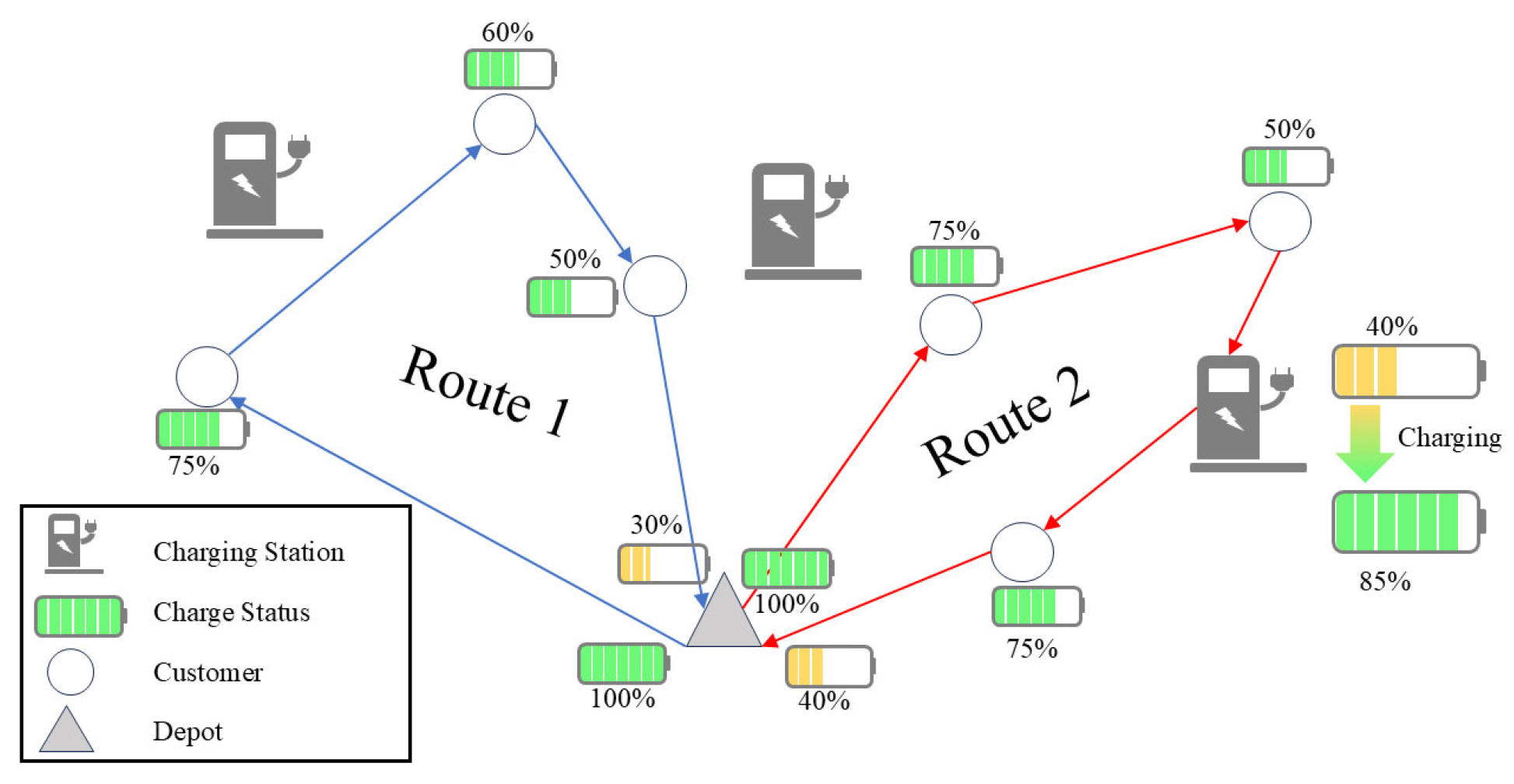
To adapt to diverse real-world application scenarios, the EVRP has been extended into numerous specialized variants. At its core, these developments consistently focus on optimizing the routing and charging behaviors of all EVs within the transportation system, by explicitly accounting for the performance characteristics of EVs and the operational attributes of CSs.

Regarding the impact of EV performance on transportation planning, existing research has comprehensively accounted for the operational characteristics of EVs, particularly the behavior of batteries under various scenarios. For instance, studies have incorporated uncertainties in travel time and energy consumption [7,8,9] when planning routes under battery capacity constraints [10,11,12], or analyzed the linear or nonlinear effects of factors such as driving speed [13] and load weight [14] on energy consumption to develop more rational transportation plans. Additionally, some research has examined the influence of emerging technologies, such as battery state monitoring [15] and mobile charging [16], on route optimization. Given the range limitations imposed by battery capacity, EVs often require en-route energy replenishment in practical operations [17]. Consequently, a number of studies permit EVs to recharge, swap batteries, or replenish energy through other means during trips [18,19], and investigate the complex relationship between charging amount and charging duration [20,21,22].

Regarding the impact of CSs’ status on transportation planning, the accessibility and charging characteristics of stations have emerged as key research topics. Numerous studies have incorporated fast-charging stations [23] to analyze their influence on route selection, or have designed various charging strategies [24,25] to accommodate different operational scenarios. In response to environmental concerns, some studies have further distinguished CSs based on their energy sources [26], guiding EVs to prioritize the use of renewable energy to reduce carbon emissions.

While traditional EVRP research often assumes unlimited service capacity at CSs, recent studies have increasingly focused on the impact of CS capacity constraints on vehicle routing [27]. For instance, some approaches adjust routes or impose additional fees to avoid charging congestion [28,29]. Such research is of significant practical relevance, as actual charging duration and waiting time directly affect scheduling efficiency [30]. Existing methods for implementing capacity constraints typically involve limiting the total number of EVs passing through a given CS [31], adopting discrete-time controls [32,33], or applying complex nonlinear formulations [34,35], analogous to the concept of link flow capacity in traffic networks [36].

However, most existing studies fail to incorporate CS capacity constraints into a continuous-time linear model that allows EVs to flexibly decide when to start and end charging. This limitation prevents the models from fully capturing realistic operational conditions and constrains computational efficiency. Moreover, existing approaches often rely on predetermined charging strategies, which cannot dynamically adjust charging amounts based on real-time routing and SOC, thereby limiting scheduling flexibility.

To address these limitations, this study aims to develop an integrated optimization model for EV routing and charging scheduling. Under the constraints of CSs’ capacity, battery capacity, and charging time characteristics, the model employs linear formulations to enable flexible decisions on charging amounts and timing. This approach is designed to enhance the utilization of charging resources and improve overall transportation efficiency.

The main contributions of this study are summarized as follows:

(1) To address the capacity constraints imposed by the limited number of chargers at CSs, a set of linear constraints is formulated. These ensure that the number of EVs charging simultaneously does not exceed the available chargers, while clearly distinguishing between EVs in charging and waiting states.

(2) Considering the battery capacity and charging time characteristics of EVs, a linear modeling approach is adopted to allow EVs to autonomously determine their optimal charging amounts.

(3) To meet practical large-scale application needs, a heuristic solution method based on a genetic algorithm (GA) is designed, enabling the model to be efficiently solved in realistic distribution scenarios.

The remainder of this paper is structured as follows: Section 2 introduces the application scenario and notation. Section 3 presents the mathematical model. Section 4 describes the GA-based heuristic solution approach. Section 5 validates the model’s effectiveness using small-scale network instances, compares its performance with existing methods, and demonstrates the algorithm’s scalability under large-scale demand. Finally, Section 6 concludes the paper.

2. Problem Formulation

2.1. Scenario and Network

Building upon the classical EVRP, the transportation network considered in this study can be represented as a graph (V, E), where V denotes the set of all nodes and E the set of all links. The node set V consists of one depot, a set of customer nodes, and a set of CSs. All EVs depart from the depot, deliver goods to their assigned customer nodes, and must finally return to the same depot.

As illustrated in Figure 1, the network comprises one depot (denoted as N₀), multiple customer points (set N), and several CSs (set I). Each feasible vehicle route starts and ends at the depot, visiting a subset of customer points and CSs along the way. The objective of this study is to simultaneously optimize the routing and charging schedules of all EVs while satisfying all customer demands, EV capacity limits, battery capacity constraints, CSs’ capacity restrictions, and other relevant conditions, with the aim of minimizing the total completion time of the transportation tasks.

2.2. Basic Assumptions and Notation

To establish the mathematical model, the following basic assumptions are adopted:

(1) Each EV departs from the depot with a fully charged battery.

(2) The service time at customer nodes is sufficiently short and can be neglected.

(3) The energy consumption of an EV is linearly proportional to its travel distance.

(4) The charging duration at a CS is linearly proportional to the amount of energy replenished.

(5) The remaining battery SOC of an EV must remain non-negative throughout its travel and any stationary periods.

The sets, parameters, and decision variables used in the model are summarized in

Table 1. Summary of notation.

Category	Notation	Description
Set	V	Set of all nodes
	E	Set of all links
	N	Set of all customer nodes
	I	Set of all CSs
	I′	Set of all virtual nodes
	K	Set of all EVs
Parameter	N0	Depot node
	$\gamma$	Energy Consumption Rate
	$C_V$	Vehicle Capacity
	M	A large penalty constant
	B	Battery Capacity
	$\mu$	Charging Speed
	V	Vehicle Speed
	$d_{ij}$	Distance from node i to node j
	$C_I$	Capacity (number of chargers) of each CS
	$D_i$	Demand at customer node i
Variables	${\alpha }_i^{lk}$	Binary, equals 1 if EV k arrives earlier than EV l at CS i
	${\beta }_i^{lk}$	Binary, equals 1 if EV l arrives after EV k has departed from CS i
	$m_i^{kl}$	Binary, equals 1 if EV l arrives before EV k departs from CS i
	$x_{ij}^k$	Binary, equals 1 if EV k travels on link (i, j)
	$y_i^k$	Binary, equals 1 if EV k charges at CS i
	${DT}_i^k$	Departure time of EV k from node i
	${AT}_i^k$	Arrival time of EV k at node i
	$R_i^k$	Battery SOC of EV k when departing from node i
	$r_i^k$	Battery SOC of EV k when arriving at node i
	T	Total task completion time of the transportation system

.

3. Model Formulation

When constructing a precise mathematical model, it is necessary to systematically address three interrelated core challenges arising from the physical characteristics of EVs and the scarcity of charging resources:

(1) Accurate Formulation of the capacity constraints of CSs: How to express the hard constraint of “a limited number of chargers” in linear form within a continuous-time domain, while clearly distinguishing among the three EV states: charging, waiting, and merely passing through.

(2) Design of Flexible Charging Decisions: How to model the consumption and replenishment of energy within a linear framework, and allow EVs to autonomously and continuously determine their optimal charging amounts based on their subsequent routes, rather than following preset rules such as full recharge or charge to a fixed threshold.

(3) Seamless Integration of Waiting Time: How to naturally incorporate waiting time caused by the capacity constraints of CSs into the EV’s travel timeline, ensuring that waiting times at virtual nodes, charging times at CSs, and travel times on arcs form a feasible temporal sequence.

It should be noted that the constraints formulated in Section 3.1, Section 3.2 and Section 3.3 are developed specifically in this study to address the challenges of CS capacity constraints, flexible charging decisions, and waiting time integration. As these formulations constitute part of the main contributions of this work, they do not directly reference existing literature. In contrast, the complete EVRP model presented in Section 3.4 is constructed by incorporating these newly developed constraints into the classical EVRP modeling framework, drawing upon established studies in the field [6].

Section 3.1, Section 3.2 and Section 3.3 below elaborate in detail on the modeling approaches designed to address each of these three challenges. Finally, in Section 3.4, these components are integrated into a complete mixed-integer linear programming model.

3.1. Modeling Charging Station Capacity Constraints

The capacity constraint of a CS implies an upper limit on the number of EVs that can charge simultaneously at the CS. If the number of EVs arriving within a certain period exceeds this limit, later arrivals must wait until a charger becomes available. In a practical transportation network, some CSs are located at traffic hubs, and EVs may pass through these CSs merely to optimize their travel route without the intention of replenishing energy. Therefore, when modeling this constraint, an EV must satisfy two conditions to be considered: its route must include the CS node, and it must actually perform charging at that node.

To distinguish whether an EV merely passes through a CS or actually charges there, we define a binary variable $y_i^k$ that equals 1 if EV k charges at CS i, and 0 otherwise. Simultaneously, let $x_{ij}^k$ be a binary variable indicating whether EV k travels from node i to node j (1 if yes, 0 otherwise).

Then, EV k can only perform charging at CS i if it arrives at that CS. This logical relationship can be expressed as:

$$y_i^k⩽\sum _{j\in \mathit{V}}{x}_{ji}^k,\forall i\in \mathit{I},k\in \mathit{K}.$$

(1)

Furthermore, as previously mentioned, due to CS capacity constraints, some arriving EVs may need to wait until an available charger becomes accessible. If waiting and charging durations are directly considered simultaneously at the same node, it becomes difficult to clearly distinguish and mathematically express these two states.

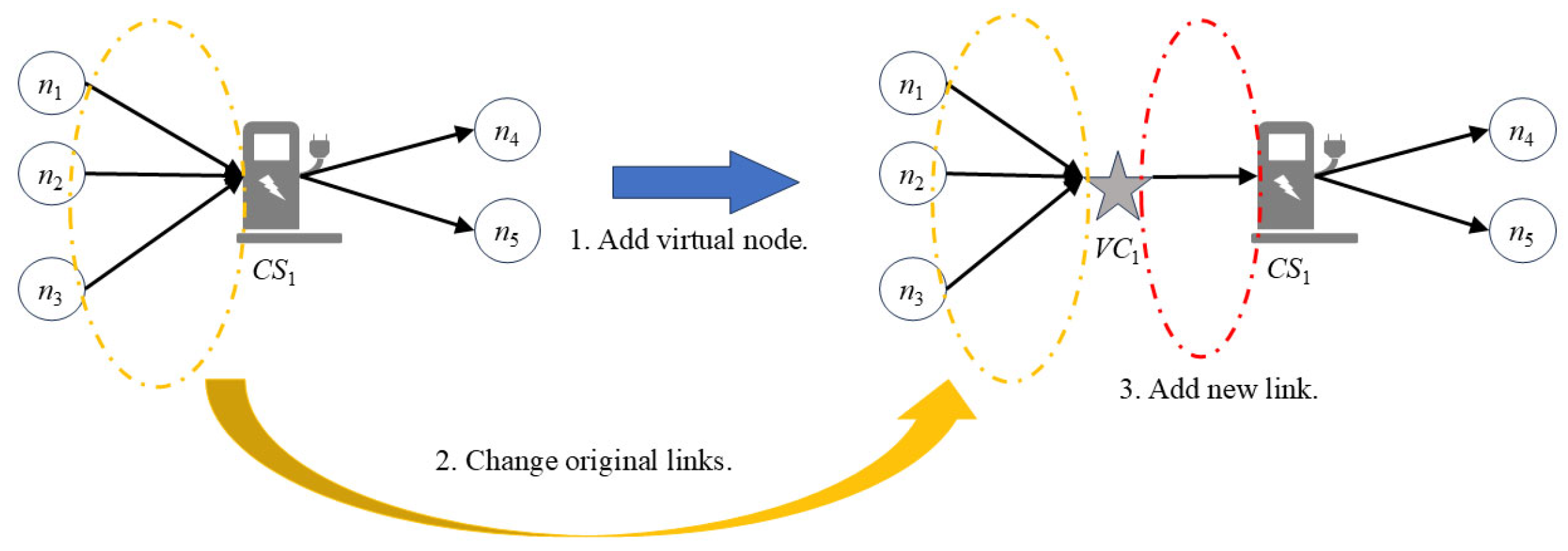
To address this, this study introduces a virtual node for each CS. Specifically, all connections originally directed toward the CS are redirected to its corresponding virtual node, while outgoing connections from the CS remain unchanged. A unidirectional link is then added between the virtual node and the CS. This network reconstruction process is illustrated in Figure 2.

Taking Figure 2 as an example, the process of adding a virtual node is as follows: For the CS node CS₁, in the original network, nodes n₁, n₂, and n₃ have links to CS₁, and CS₁ has outgoing links to n₄ and n₅. First, a virtual node VC₁ corresponding to CS₁ is added. Then, the links from n₁, n₂, and n₃ to CS₁ are redirected to VC₁. Finally, a new link from VC₁ to CS₁ is created. Through these three steps, the network restructuring is completed.

The set of added virtual nodes is denoted by I′, The waiting time incurred due to the unavailability of an idle charger at a CS occurs exclusively at the corresponding virtual node. This implies that when an EV passes through the virtual node and reaches the associated CS, it can begin charging immediately and depart the CS once charging is completed.

Specifically, if an EV’s route includes both a CS and its virtual node, the EV starts waiting upon arriving at the virtual node, and its departure from the virtual node to the corresponding CS indicates that a charger has become available. The arrival of the EV at the CS is treated as the start of charging, while its departure from the CS marks the completion of charging. In practice, if an EV arrives at a CS when a charger is already idle, this is represented in the model as a zero waiting time at the virtual node, meaning the EV can start charging immediately upon arrival.

It should be noted that if a vehicle merely passes through a CS without charging there, it will be modeled as “passing through” both the virtual node and the CS, meaning it only visits the node as part of its route, without incurring any waiting or charging time.

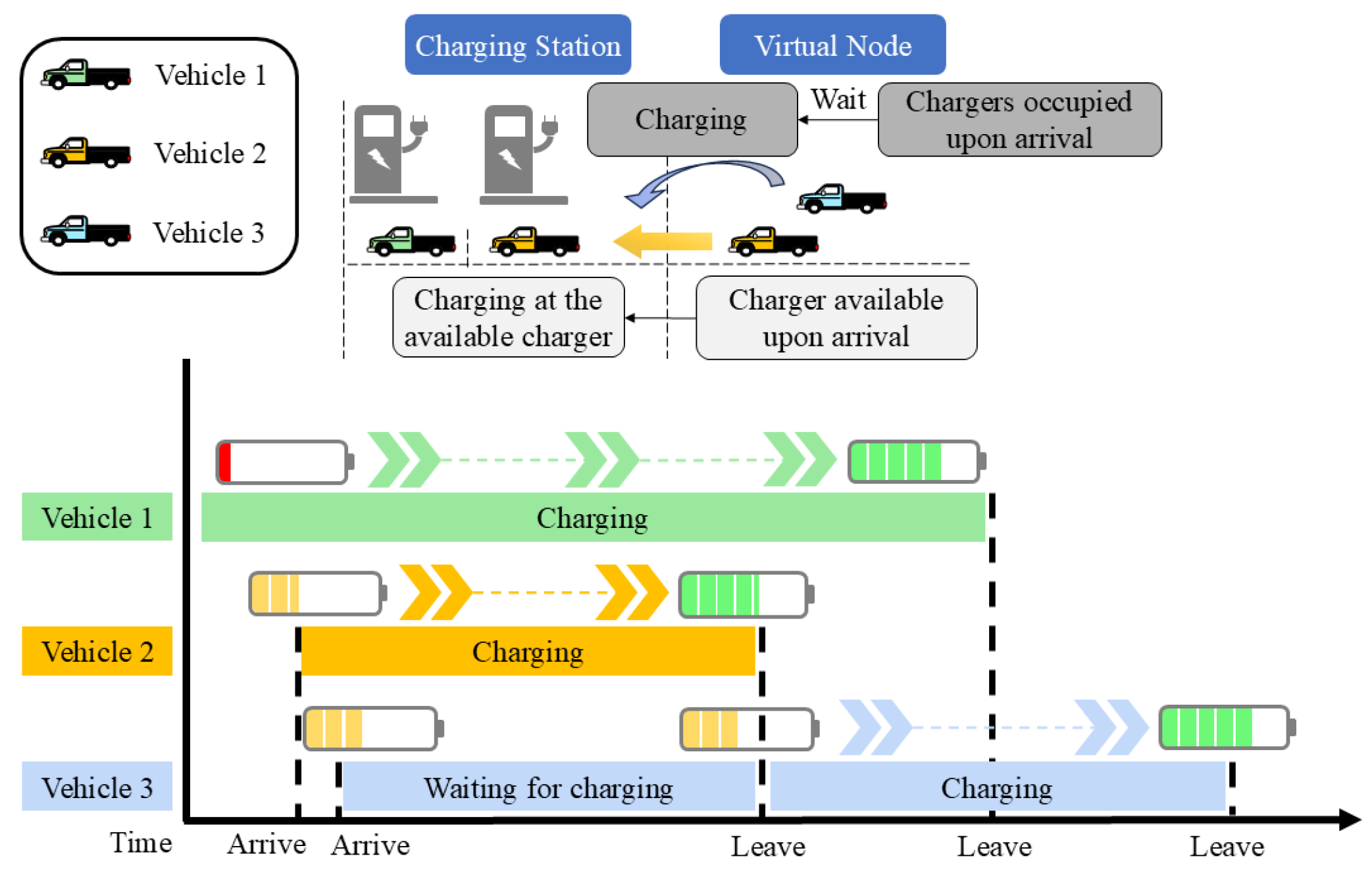
In summary, for the restructured network, the total number of EVs charging simultaneously at any CS must not exceed the total number of chargers available at that CS, denoted by $C_I$. When an EV arrives at a virtual node, if all chargers at the corresponding CS are occupied, the newly arrived EV must wait until a charger becomes available, as illustrated in Figure 3.

As shown in Figure 3, the CS has two chargers, with Vehicle 1 initially occupying one of them. When Vehicle 2 arrives at the corresponding virtual node, an idle charger is available at the station, allowing Vehicle 2 to proceed immediately from the virtual node to the station to start charging. In this case, Vehicle 2 merely passes through the virtual node without waiting. Vehicle 3 arrives slightly later at the same virtual node, at which point no charger is available. Vehicle 3 must therefore wait at the virtual node (with its battery SOC unchanged) until Vehicle 2 completes charging and releases a charger, after which it can proceed to the station.

With the introduction of virtual nodes, if a vehicle stays at a virtual node, it indicates that the vehicle needs to charge at the corresponding station but finds no available charger upon arrival. If a vehicle merely passes through a virtual node, the binary variable $y_i^k$ distinguishes whether it proceeds to charge or simply passes by the station.

This implies that for any EV that chooses to charge at a given CS, the difference between the number of EVs that enter the CS to charge during its charging period and the number of EVs that finish charging and leave during the same period must not exceed $C_I-1$ (since the EV itself occupies one charger). Formally, let ${\gamma }_1$ denote the total number of EVs that start charging at the CS after this EV begins its own charging, and let ${\gamma }_2$ represent the total number of EVs that start charging at the CS before this EV finishes its own charging. Then, the following relationship must hold:

$${\gamma }_1-{\gamma }_2⩽C_I-1,\forall i\in \mathit{I}.$$

(2)

To clearly apply the above condition to all EVs and enable each EV to check the constraint by comparing arrival and departure times, it is necessary to define several auxiliary variables that determine the temporal order of events.

To compare the arrival sequence of EVs charging at CS i, a binary variable ${\alpha }_i^{lk}$ is introduced. For CS i, ${\alpha }_i^{lk}$ equals 1 if EV l arrives later than EV k, (both requiring charging at i), and 0 otherwise. This relationship can be expressed as:

$$A{T}_i^k-A{T}_i^l\le M\cdot \left(1-{\alpha }_i^{lk}\right),\forall i\in \mathit{I},k,l\in \mathit{K},k\ne l,$$

(3)

$$A{T}_i^l-A{T}_i^k\le M\cdot \left(1-{\alpha }_i^{kl}\right),\forall i\in \mathit{I},k,l\in \mathit{K},k\ne l.$$

(4)

To ensure that the variables ${\alpha }_i^{kl}$ and ${\alpha }_i^{lk}$ correctly reflect the arrival order when EVs k and l both charge at the same CS i, the following condition must be satisfied: the sum of the two variables must be greater than or equal to 1 (indicating that one EV necessarily arrives before the other). In all other cases, when at least one of the two EVs does not charge at CS i, their sum should be less than 1 (as order comparison is redundant). That is, through the variable $y_i^k$ only EVs that actually charge at the station are considered within the capacity constraints, while vehicles that merely pass through are excluded:

$${\alpha }_i^{kl}+{\alpha }_i^{lk}\ge y_i^k+y_i^l-1,\forall i\in \mathit{I},k,l\in \mathit{K},k\ne l,$$

(5)

$${\alpha }_i^{kl}+{\alpha }_i^{lk}\le {\displaystyle \frac{y_i^k+y_i^l}{2}},\forall i\in \mathit{I},k,l\in \mathit{K},k\ne l.$$

(6)

Furthermore, it is necessary to ensure that the arrival sequence of EVs charging at CS i does not form a cycle (e.g., where k arrives before l, l before h, h before k, which would be illogical). This condition can be expressed by the following relation:

$${\alpha }_i^{kl}+{\alpha }_i^{lh}+{\alpha }_i^{hk}⩾y_i^k+y_i^l+y_i^h-2,\forall i\in \mathit{I},k,l,h\in \mathit{K},k\ne l\ne h.$$

(7)

To analyze the number of EVs that arrive at CS i for charging before a given EV finishes and departs, an auxiliary variable ${\beta }_i^{lk}$ is introduced. For CS i, ${\beta }_i^{lk}$ equals 1 if EV l (requiring charging) arrives after EV k has completed charging and departed; otherwise, it is 0. This relationship can be expressed as:

$$D{T}_i^k-A{T}_i^l\le M\cdot \left(1-{\beta }_i^{lk}\right),\forall i\in \mathit{I},k,l\in \mathit{K},k\ne l.$$

(8)

To analyze the number of EVs that arrive at CS i for charging before a given EV finishes and departs, a variable $m_i^{kl}$ is introduced. For CS i, $m_i^{kl}$ equals 1 if EV l (which requires charging) arrives before EV k completes charging and departs; otherwise, it is 0. This relationship can be expressed as:

$$A{T}_i^l-D{T}_i^k\le M\cdot \left(1-m_i^{kl}\right),\forall i\in \mathit{I},k,l\in \mathit{K},k\ne l.$$

(9)

To ensure that the variables ${\beta }_i^{lk}$ and $m_i^{kl}$ correctly reflect the temporal relationship when EVs k and l both charge at the same CS i, the following condition must be satisfied: the sum of the two variables must be greater than or equal to 1 (indicating that EV l arrives either before or after EV k departs, only these two possibilities exist). In all other cases, when at least one of the two EVs does not charge at CS i, their sum should be less than 1 (since order comparison is irrelevant). That is:

$${\beta }_i^{lk}+m_i^{kl}\ge y_i^k+y_i^l-1,\forall i\in \mathit{I},k,l\in \mathit{K},k\ne l.$$

(10)

$${\beta }_i^{lk}+m_i^{kl}\le {\displaystyle \frac{y_i^k+y_i^l}{2}},\forall i\in \mathit{I},k,l\in \mathit{K},k\ne l.$$

(11)

By integrating these newly introduced variables, the capacity constraint in Equation (2) can be specified as a set of constraints for each CS and each EV, expressed as follows:

$$\sum _l{\alpha }_i^{lk}-\sum _l{\beta }_i^{lk}\le C_I-1,\forall i\in \mathit{I},k\in \mathit{K}.$$

(12)

Through Equations (3)–(12), a complete mathematical representation of the CS capacity constraint can be formulated and enforced throughout the entire transportation task.

3.2. Modeling Flexible Charging Decisions

As stated in assumption (3) of Section 2.2, this study assumes a linear relationship between energy consumption and travel distance. Existing studies have investigated the effects of factors such as driving speed [13] and load weight [14] on energy consumption, and have developed various battery state monitoring technologies for more accurate battery status feedback [37,38]. However, the primary focus of this study is on addressing CS capacity constraints and flexible charging decisions. Therefore, following the approach of several established EVRP studies [6,15], we adopt this linear assumption to concentrate on the core contributions of our work.

Let $r_i^k$ denote the remaining battery SOC of EV k upon arriving at node i. For any customer node i in the transportation network, the battery SOC $r_i^k$ when the EV departs from that node (which, for a customer node, is assumed equal to the battery SOC upon arrival) minus the energy consumed during travel equals the battery SOC $r_j^k$ upon reaching the next node j. This relationship can be expressed as:

$$r_j^k⩽r_i^k-\gamma \cdot d_{ij}\cdot x_{ij}^k+B\left(1-x_{ij}^k\right),\forall i\in N,k\in \mathit{K},\left(i,j\right)\in \mathit{E}.$$

(13)

where B is the maximum battery capacity of the EV, $d_{ij}$ is the travel distance from node i to node j, and $\gamma$ is the energy consumption per unit distance traveled.

It is worth noting that this study assumes all EVs start from the depot with a fully charged battery. This condition can be expressed as:

$$r_j^k⩽B-\gamma \cdot d_{ij}\cdot x_{ij}^k+B\left(1-x_{ij}^k\right),i=N_0,\forall k\in \mathit{K},\left(i,j\right)\in \mathit{E}.$$

(14)

For a CS i, an EV can replenish its battery upon arrival. Therefore, the battery SOC upon departure needs to be distinguished from that upon arrival. Let $R_i^k$ represent the battery SOC of EV k when it departs from CS i. Then, the battery SOC $R_i^k$ when leaving CS i, minus the energy consumed during travel equals the battery SOC $r_j^k$ upon arriving at the next node j. This relationship can be expressed as:

$$r_j^k⩽R_i^k-\gamma \cdot d_{ij}\cdot x_{ij}^k+B\left(1-x_{ij}^k\right),\forall i\in \mathit{I},k\in \mathit{K},\left(i,j\right)\in \mathit{E}.$$

(15)

During the charging process of an EV, this study assumes a linear relationship between charging duration and the required charging amount. Consequently, the time required for charging can be derived from the difference between the EV’s battery SOC upon arrival at and departure from the CS. The specific expression is as follows:

$${AT}_i^k+\mu \cdot \left(R_i^k-r_i^k\right)-D{T}_i^k⩽M\cdot \left(1-\sum _{j\in \mathit{N}}{x}_{ij}^k\right),\forall i\in \mathit{I},k\in \mathit{K}.$$

(16)

where ${AT}_i^k$ denotes the arrival time of EV k at node i, ${DT}_i^k$ represents the departure time of EV k from node i (this variable is defined only for the depot, CSs, and their virtual nodes in the transportation network), and $\mu$ is the time required to replenish one unit of energy.

Since EV k may merely pass through CS i without charging, the SOC upon departure needs to be constrained according to the binary charging decision variable $y_i^k$. Specifically, the lower bound of the battery SOC when EV k departs from CS i is the SOC upon arrival. This relationship can be expressed as:

$$R_i^k⩾r_i^k,\forall i\in \mathit{I},k\in \mathit{K}.$$

(17)

When EV k charges at CS i, the battery SOC upon departure will exceed this lower bound; otherwise, it will remain exactly equal to the battery SOC upon arrival. This relationship can be expressed as:

$$R_i^k-r_i^k⩽M\cdot y_i^k,\forall i\in \mathit{I},k\in \mathit{K}.$$

(18)

It should be noted that constraint (18) serves to distinguish whether an EV merely passes through a CS without charging. Combined with the treatment in Section 3.1, where vehicles that merely pass through are excluded from capacity constraints via the variable $y_i^k$, EVs that only pass by a CS will neither replenish energy nor experience waiting at the virtual node due to capacity limitations.

Throughout the transportation process, the SOC of EV k when departing from any CS or the depot, as well as when arriving at any node in the network, must not exceed the battery capacity upper limit. This condition can be expressed as:

$$R_i^k⩽B,\forall i\in \mathit{I}\cup N_0,k\in \mathit{K},$$

(19)

$$r_i^k⩽B,\forall i\in \mathit{N}\cup \mathit{I}\cup {\mathit{I}}^{\prime }\cup N_0,k\in \mathit{K}.$$

(20)

Equations (13)–(20) provide rigorous mathematical constraints that govern the battery dynamics of EVs at CSs and their relationship to travel time.

3.3. Modeling Waiting Time in Charging Stations

When an EV travels to a CS to recharge, if all chargers at the CS are occupied, the EV must first wait at the corresponding virtual node until a charger becomes available before starting to charge. To analyze the waiting time at the virtual node, it is first necessary to establish the travel time constraints during the transportation process.

In the transportation network, it is assumed that after an EV arrives at any customer node i, it departs for the next node after a negligible and ignorable duration. Therefore, only the arrival time is recorded at a customer node, and the travel time from that node to the next node is entirely determined by the distance of the road, expressed as:

$$A{T}_i^k+{\displaystyle \frac{d_{ij}}{V}}-A{T}_j^k⩽M\cdot \left(1-x_{ij}^k\right),\forall i\in \mathit{N},\left(i,j\right)\in \mathit{E},k\in \mathit{K},$$

(21)

$$A{T}_j^k-{\displaystyle \frac{d_{ij}}{V}}-A{T}_i^k⩽M\cdot \left(1-x_{ij}^k\right),\forall i\in \mathit{N},\left(i,j\right)\in \mathit{E},k\in \mathit{K}.$$

(22)

For CSs and their virtual nodes in the transportation network, the departure time of an EV from such a node and its arrival time at the next node are both related to the travel distance, i.e.,

$$D{T}_i^k+{\displaystyle \frac{d_{ij}}{V}}-A{T}_j^k⩽M\cdot \left(1-x_{ij}^k\right),\forall i\in \mathit{I}\cup {\mathit{I}}^{\prime },\left(i,j\right)\in \mathit{E},k\in \mathit{K},$$

(23)

$${AT}_j^k-{\displaystyle \frac{d_{ij}}{V}}-{DT}_i^k⩽M\cdot \left(1-x_{ij}^k\right),\forall i\in \mathit{I}\cup {\mathit{I}}^{\prime },\left(i,j\right)\in \mathit{E},k\in \mathit{K}.$$

(24)

For any virtual node, the lower bound of its departure time is the arrival time at that node, that is:

$$A{T}_i^k-D{T}_i^k⩽M\cdot \left(1-\sum _{j\in \mathit{N}\cup \left\{N_0\right\}}{x}_{ji}^k\right),\forall i\in {\mathit{I}}^{\prime },k\in \mathit{K}.$$

(25)

To construct complete constraints for the departure and arrival times of EV k at a virtual node using the binary charging decision variable, let $F_i$ denote the index of the CS corresponding to virtual node i. Only when EV k charges at CS $F_i$ can its departure time from virtual node i be later than its arrival time due to waiting; otherwise, the two times must be equal. This relationship can be expressed as:

$$D{T}_i^k-A{T}_i^k⩽M\cdot y_{F_i}^k,\forall i\in {\mathit{I}}^{\prime },k\in \mathit{K}.$$

(26)

Equations (21)–(26) provide rigorous mathematical constraints linking the travel time of EVs during transportation with their charging decisions at CSs.

3.4. Optimization Model Building

Equations (1) and (3)–(26) provide the mathematical modeling foundation for addressing the challenges posed by CS capacity and EV battery capacity constraints. Since capacity limitations at CSs may lead to additional waiting time and the charging process itself consumes time, the objective of vehicle route optimization should be formulated as minimizing the total task completion time. Let T denote the time required for all EVs in the transportation system to complete their tasks. The objective function of this study can thus be set as minimizing T, where T must be no less than the latest return time among all EVs to the depot, i.e.,

$$A{T}_{N_0}^k⩽T,\forall k\in \mathit{K}.$$

(27)

Furthermore, in the EV schedule, it is assumed that all EVs depart from the depot at time zero, and the arrival time at the depot records the moment when an EV returns after completing its task. As a result, Equations (21)–(24) cannot accurately describe the departure time of an EV from the depot. Therefore, an additional description is needed for this scenario, which can be expressed as:

$$0+{\displaystyle \frac{d_{ij}}{V}}-A{T}_j^k⩽M\cdot \left(1-x_{N_{0}j}^k\right),\forall j\in \left\{j\left|\left(N_0,j\right)\in \mathit{E}\right.\right\}.$$

(28)

For customer nodes, CSs, and virtual nodes in the transportation network, EVs depart after arriving. This condition can be expressed as:

$$\sum _{j\in \left\{j\left|\left(\mathrm{i},j\right)\in \mathit{E}\right.\right\}}{x}_{ij}^k-\sum _{j\in \left\{j\left|\left(j,i\right)\in \mathit{E}\right.\right\}}{x}_{ji}^k=0,\forall i\in \mathit{N}\cup \mathit{I}\cup {\mathit{I}}^{\prime },k\in \mathit{K}.$$

(29)

In addition, it must be ensured that each EV departs from the depot at most once, that no node is visited more than once along a route, that each customer node is served by exactly one EV, and that CSs may be visited by multiple EVs. Furthermore, since each customer point i has a non-negative demand $D_i$, the total demand served by any EV must respect its vehicle capacity limit. These constraints can be expressed as:

$$\sum _{j\in \left\{j\left|\left(N_0,j\right)\in \mathit{E}\right.\right\}}{x}_{N_{0}j}^k⩽1,\forall k\in \mathit{K},$$

(30)

$$\sum _{j\in \left\{j\left|\left(j,i\right)\in \mathit{E}\right.\right\}}{x}_{ji}^k⩽1,\forall i\in \mathit{N}\cup \mathit{I}\cup {\mathit{I}}^{\prime },k\in \mathit{K},$$

(31)

$$\sum _{k\in \mathit{K}}\sum _{j\in \left\{j\left|\left(j,i\right)\in \mathit{E}\right.\right\}}{x}_{ji}^k=1,\forall i\in \mathit{N},$$

(32)

$$\sum _{i\in \mathit{N}}{D}_i\sum _{j\in \left\{j\left|\left(i,j\right)\in \mathit{E}\right.\right\}}{x}_{ji}^k⩽C_V,\forall k\in \mathit{K}.$$

(33)

In summary, the EVRP model considering CS capacity and EV battery capacity constraints can be formulated as follows. To minimize the maximum task completion time while controlling the total number of vehicles used, the total travel time of all vehicles should be incorporated into the objective function. This prevents excessive vehicle dispatch for the purpose of reducing the maximum completion time. The objective function can be expressed as:

$$\mathrm{m}\mathrm{i}\mathrm{n} T+\sum _{\left(i,j\right)\in \mathit{E}}{\displaystyle \frac{d_{ij}}{V}}\sum _{k\in \mathit{K}}{x}_{ij}^k$$

(34)

Subject to Equations (1) and (3)–(33), and:

$$x_{ij}^k\in \left\{\mathrm{0,1}\right\},\forall \left(i,j\right)\in \mathit{E},k\in \mathit{K}$$

(35)

$$A{T}_i^k⩾0,\forall i\in \mathit{N}\cup \mathit{I}\cup {\mathit{I}}^{\prime }\cup \left\{N_0\right\},k\in \mathit{K}$$

(36)

$${DT}_i^k⩾0,\forall i\in \mathit{I}\cup {\mathit{I}}^{\prime },k\in \mathit{K}$$

(37)

$$y_i^k\in \left\{0,1\right\},\forall i\in \mathit{I},k\in \mathit{K}$$

(38)

$$T⩾0$$

(39)

It should be noted that the specific values of the parameters in the model will be provided in Section 5 when numerical experiments are conducted.

4. Solution Algorithm

The model proposed in Section 3 describes EV charging–waiting behaviors using a large number of binary variables and extensive constraints. Consequently, when applied to instances with a high number of demand points, the required solution time may become excessively long, making it difficult to meet time-critical requirements in some scenarios. To overcome this challenge, this section develops a tailored solution algorithm based on a genetic algorithm (GA) framework. By making targeted adaptations to the charging-related behaviors of EVs, the algorithm effectively improves computational speed at the expense of some optimality. This enables the model, with the support of the algorithm, to be applicable in time-sensitive operational settings.

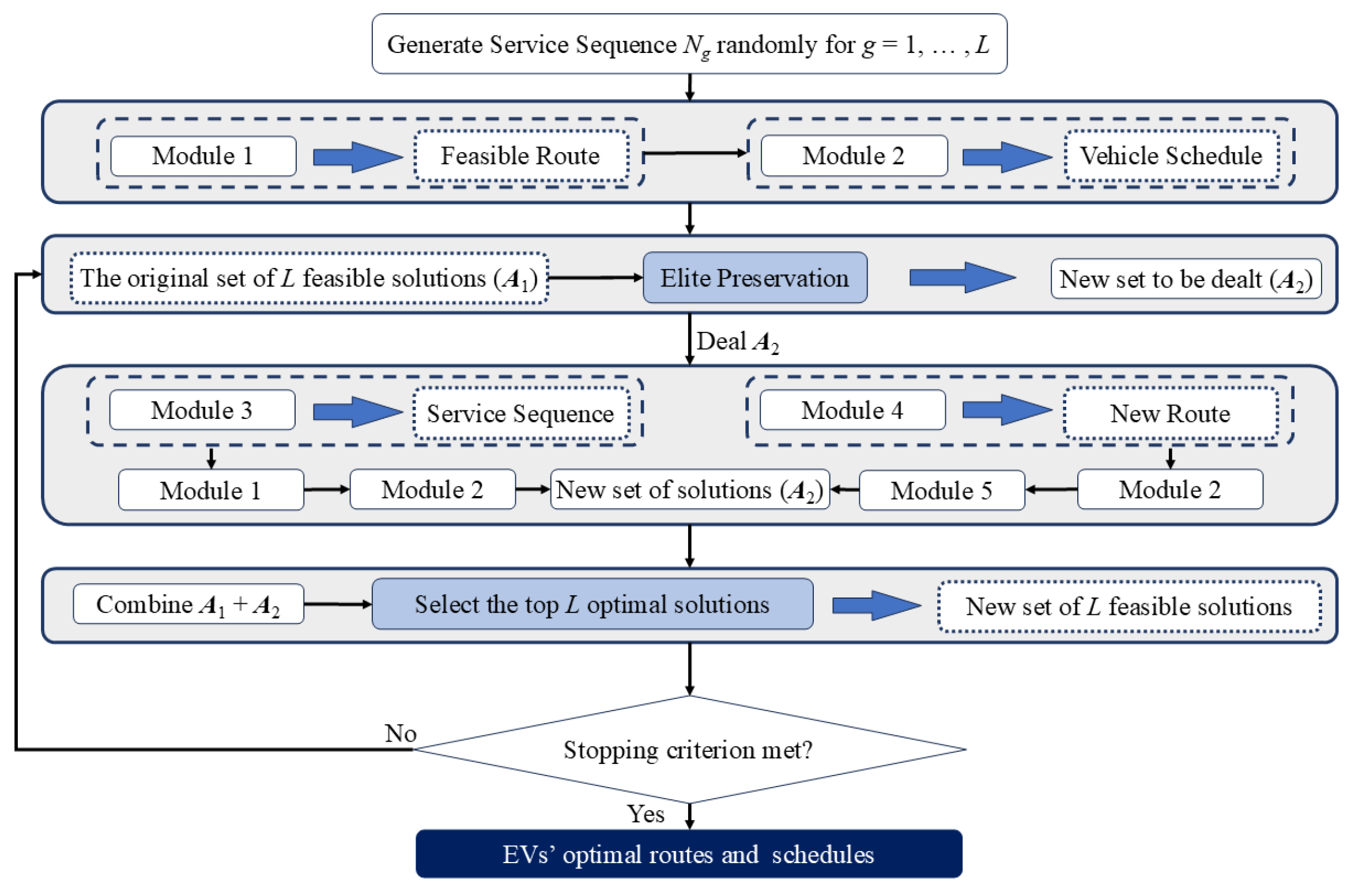
In terms of execution flow, the algorithm first takes the set of demand nodes in the network and randomly permutes it to generate multiple service sequences ${\mathit{N}}_g$ ($g=1,\cdots ,L$), where L is a preset number of feasible solutions. After initialization, a feasible route generation module (Module 1, which is implemented as Algorithm 1) is applied. By incorporating instance-specific information such as the maximum loading capacity and maximum battery capacity of EVs, Algorithm 1 processes each demand node sequence and produces feasible transportation routes that dispatch multiple EVs to serve the sequence of demand nodes in turn, while ensuring timely detours to CSs for energy replenishment. Subsequently, for each set of routes, a time computation module (Module 2, which is implemented as Algorithm 2) is invoked to compute the arrival time of each EV at every node as well as the charging duration required at CSs. Through these steps, an initial set of L feasible solutions (referred to as set A₁) is obtained.

After obtaining the initial feasible solutions, the algorithm performs a secondary processing step to explore higher-quality solutions. First, an elite preservation operation is applied, giving higher-quality solutions a greater probability of serving as the basis for generating new solutions. This procedure follows the classic genetic algorithm elite preservation scheme exactly, and the resulting set of solutions is denoted as A₂. Next, set A₂ undergoes further refinement through a service-sequence optimization module (Module 3). Module 3 generates new service sequences by locally swapping portions of the demand-node service order between two feasible solutions, after which Algorithm 1 is invoked to produce corresponding feasible transportation routes. Finally, a charging-order optimization module (Module 4) is applied to the current set of feasible route sequences. Specifically, for EVs that require charging, Module 4 adjusts the sequence in which they arrive at CSs, enabling earlier charging to avoid potential waiting congestion. After the operations of Modules 3 and 4, Algorithm 2 is called again to compute the updated arrival/departure information for all affected routes.

Furthermore, adjusting the order of arrivals at CSs may result in infeasible routes, for instance, the EV’s battery capacity may become insufficient for the remaining distance. Therefore, a feasibility-check module (Module 5) is designed to verify whether the modified route remains feasible. If the route is infeasible, its objective function value is set to a large penalty constant M, thereby reducing the likelihood that the infeasible solution is retained in subsequent iterations.

Next, sets A₁ and the processed set A₂ are merged, and the top L best solutions from the combined set are selected as the new initial solution set A₁ for the next iteration. Convergence is checked based on the change in the objective function value. If the objective function does not improve over 20 consecutive iterations, or if the maximum number of iterations is reached, the algorithm terminates and outputs the current best solution (i.e., the first solution in A₁). Otherwise, the iterative computation continues.

The flow of the algorithm is illustrated in Figure 4.

4.1. Module 1: Feasible Route Generation

This module aims to efficiently dispatch EVs based on an input sequence of demand nodes, taking into account parameters such as the loading capacity of all EVs, the demand at each node, travel distances, and energy consumption, so that the EVs can serve the demand nodes sequentially in the given order. When an EV’s remaining battery is insufficient to reach the next node, it is guided to a CS for timely energy replenishment.

To achieve this, Algorithm 1 (implementing Module 1) performs a greedy search starting from the depot. The cumulative energy consumption $E^c$ and cumulative load $Q^c$ are initialized to zero. The algorithm then proceeds along the demand node sequence ${\mathit{N}}_g$ of the g-th feasible solution. Upon arriving at node i, $E^c$ is updated and $Q^c$ is increased by the node’s demand $D_i$. If either $Q^c$ or $E^c$ indicates that the EV cannot serve the next demand node, the EV is instructed to return to the depot, directly if the remaining energy is sufficient, or via the nearest charging station $D{S}_i$ from node i, to recharge first if energy is inadequate. After returning, a new route is started again from the depot. If both $Q^c$ and $E^c$ allow travel to the next node in ${\mathit{N}}_g$, the EV proceeds to that node and the route, $Q^c$ and $E^c$ are updated accordingly.

It should be noted that for the last EV in the sequence, it must return to the depot after completing ${\mathit{N}}_g$. However, it is also necessary to check whether the remaining energy is sufficient for the return trip; if not, the EV must first visit the nearest CS to recharge before heading back to the depot.

Furthermore, because the network was modified in Section 3 by adding a unique virtual node for each CS, in the revised network an EV must pass through the corresponding virtual node $F_i$ before arriving at CS i. For EV k in the g-th feasible solution, in order to facilitate subsequent calculations, the number of nodes $P_g^k$ visited from the depot up to $F_i$ is recorded.

The above procedure can be summarized as follows.

Algorithm 1. Feasible Route Generation

Initialization: Read ${\mathit{N}}_g$, $k^c\leftarrow 0$, $Q^c\leftarrow 0$, $E^c\leftarrow 0$, $l\leftarrow 1$ $\mathit{R}\left(k^c\right)\leftarrow \left[N_0\right]$, $i\leftarrow N_0$ While l ≠ length(${\mathit{N}}_g$)         If $Q^c+D_{{\mathit{N}}_g\left[l+1\right]}⩽C_v$ and $E^c+\gamma \cdot d_{i{\mathit{N}}_g\left[l+1\right]}⩽B$                $\mathit{R}\left(k^c\right)\leftarrow \mathit{R}\left(k^c\right)\cup \left[{\mathit{N}}_g\left[l+1\right]\right]$, $Q^c\leftarrow Q^c+D_{{\mathit{N}}_g\left[l\right]}$, $E^c\leftarrow E^c+\gamma \cdot d_{i{\mathit{N}}_g\left[l+1\right]}$                $i\leftarrow {\mathit{N}}_g\left[l+1\right]$, $l\leftarrow l+1$                If $l=length\left({\mathit{N}}_g\right)$                      If $E^c+\gamma \cdot d_{i{\mathit{N}}_0}⩽B$                             $P_g^{k^c}\leftarrow length\left(\mathit{R}\left(k^c\right)\right)+1$, $\mathit{R}\left(k^c\right)\leftarrow \mathit{R}\left(k^c\right)\cup \left[F_{D{S}_i},D{S}_i,N_0\right]$                      Else                             $\mathit{R}\left(k^c\right)\leftarrow \mathit{R}\left(k^c\right)\cup \left[N_0\right]$         Else                If $E^c+\gamma \cdot d_{i{\mathit{N}}_0}⩽B$                      $P_g^{k^c}\leftarrow length\left(R\left(k^c\right)\right)+1$, $\mathit{R}\left(k^c\right)\leftarrow \mathit{R}\left(k^c\right)\cup \left[F_{D{S}_i},D{S}_i,N_0\right]$                Else                      $\mathit{R}\left(k^c\right)\leftarrow \mathit{R}\left(k^c\right)\cup \left[N_0\right]$                 $k^c\leftarrow k^c+1$, $Q^c\leftarrow 0$, $E^c\leftarrow 0$, $\mathit{R}\left(k^c\right)\leftarrow \left[N_0\right]$, $i\leftarrow N_0$

4.2. Module 2: Arrival and Departure Time Computation

This module generates detailed information for each EV k at every node i—including remaining battery SOC $r_{ik}$, arrival time, and departure time, based on the given vehicle routes and the number of chargers at each CS.

To achieve this, Algorithm 2 (implementing Module 2) executes the following three core steps:

Step 1: Preliminary time and energy profile

For each dispatched EV in the g-th solution, the EV departs from the depot at time zero with a full battery B. Following the node-visit sequence and the distance of each traversed link, travel times are accumulated to determine the arrival and departure times at every node. Concurrently, the energy consumed along each link is deducted to compute the battery SOC $r_{ik}$ when EV k arrives at node i and the battery SOC $R_{ik}$ when it departs.

Step 2: Charging necessity and duration determination

Based on the remaining battery SOC when the EV returns to the depot, a check is performed to determine whether charging is required. If the remaining SOC is less than or equal to zero, charging is necessary; otherwise, the EV proceeds without charging. When charging is needed, a greedy criterion is applied: the ideal charging amount is calculated so that the EV returns to the depot with exactly zero residual energy. Using the charging-time coefficient, the required charging duration is derived. The arrival/departure times and SOC for the return leg from the CS to the depot are then updated accordingly.

Step 3: Charging scheduling under capacity constraints

EVs that charge at the same CS are sorted by their planned charging start times. For each charging EV, the number of EVs that start charging during its charging interval is counted. If this number exceeds the number of chargers at the CS, later-arriving EVs are delayed, i.e., their departure from the corresponding virtual node is postponed, until the earliest-charging EV finishes and a charger becomes available.

Example: Suppose EV k is charging at CS i, which has three chargers, and EVs l and m arrive and start charging during k’s charging period. Then, any later-arriving EV h must wait at the virtual node until the earliest among k, l, m completes charging before it can begin.

The above procedure can be summarized as follows.

Algorithm 2. Arrival and Departure Computation

For k = 0: $k^c$−1        $A{T}_{N_0}^k\leftarrow 0$, $D{T}_{N_0}^k\leftarrow 0$, $r_{N_0}^k\leftarrow B$, $R_{N_0}^k\leftarrow B$        For l = 2: length($\mathit{R}\left(k\right)$)               $i\leftarrow \mathit{R}\left(k\right)\left[l-1\right]$, $j\leftarrow \mathit{R}\left(k\right)\left[l\right]$               $A{T}_j^k\leftarrow A{T}_i^k+{\displaystyle \frac{d_{ij}}{v}}$, $D{T}_j^k\leftarrow D{T}_i^k+{\displaystyle \frac{d_{ij}}{v}}$, $r_j^k\leftarrow r_i^k-\gamma \cdot d_{ij}$, $R_j^k\leftarrow R_i^k-\gamma \cdot d_{ij}$        If $r_{N_0}^k<0$               $T^{en}\leftarrow -\mu \cdot r_{N_0}^k$, $E^n\leftarrow -r_{N_0}^k$               For l = length($\mathit{R}\left(k\right)$): 2                       $i\leftarrow \mathit{R}\left(k\right)\left[l-1\right]$                       $D{T}_i^k\leftarrow D{T}_i^k+T^{en}$, $R_i^k\leftarrow R_i^k+E^n$                       If $i\notin \mathit{I}$                             $A{T}_i^k\leftarrow A{T}_i^k+T^{en}$, $r_i^k\leftarrow r_i^k+E^n$                       Else                             Break For $i\in \mathit{I}$       $\mathit{V}\leftarrow \left[ \right]$, $\mathit{A}\leftarrow \left[ \right]$, $\mathit{D}\leftarrow \left[ \right]$       For k = 0: $k^c$−1               If $i\in \mathit{R}\left(k\right)$                      $\mathit{V}\leftarrow \mathit{V}\cup \left[k\right]$, $\mathit{A}\leftarrow \mathit{A}\cup \left[A{T}_i^k\right]$, $\mathit{D}\leftarrow \mathit{D}\cup \left[D{T}_i^k\right]$       If length(V) > $C_I$              Sort array A in ascending order and adjust the corresponding elements in vectors V and D according to the changes in element indices.              For l = 1 : length(A) − 1                      $V^{now}\leftarrow 0$                      For m = l +1: length(A)                              If $\mathit{A}\left[m\right]⩾\mathit{D}\left[l\right]$                                       Break                              Else                                      $V^{now}\leftarrow V^{now}+1$                                      If $V^{now}>C_I$                                              $T^{en}\leftarrow \mathit{D}\left[l\right]-\mathit{A}\left[m\right]$, $\mathit{A}\left[m\right]\leftarrow \mathit{D}\left[l\right]$, $\mathit{D}\left[m\right]\leftarrow \mathit{D}\left[m\right]+T^{en}$                                              $j\leftarrow j\left|\mathit{R}\left(\mathit{V}\left[m\right]\right)\left[j\right]\right.=i$, $D{T}_{\mathit{R}\left(\mathit{V}\left[m\right]\right)\left[j-1\right]}^{\mathit{V}\left[m\right]}\leftarrow D{T}_{\mathit{R}\left(\mathit{V}\left[m\right]\right)\left[j-1\right]}^{\mathit{V}\left[m\right]}+T^{en}$                                              For h = j + 1: length($\mathit{R}\left(\mathit{V}\left[m\right]\right)$)                                                      $A{T}_{\mathit{R}\left(\mathit{V}\left[m\right]\right)\left[h\right]}^{\mathit{V}\left[m\right]}\leftarrow A{T}_{\mathit{R}\left(\mathit{V}\left[m\right]\right)\left[h\right]}^{\mathit{V}\left[m\right]}+T^{en}$                                                      $D{T}_{\mathit{R}\left(\mathit{V}\left[m\right]\right)\left[h\right]}^{\mathit{V}\left[m\right]}\leftarrow D{T}_{\mathit{R}\left(\mathit{V}\left[m\right]\right)\left[h\right]}^{\mathit{V}\left[m\right]}+T^{en}$

4.3. Module 3: Service-Sequence Optimization

This module is designed based on the crossover principle of genetic algorithms. Its main function is to exchange segments of the service sequences between the g-th and (g + 1)-th solutions, both of which have undergone elite preservation, with the earlier-ranked solutions being of higher quality. This operation expands the set of EV routes, enabling the exploration of potentially better transportation plans.

The module is triggered with a preset probability p₁. Specifically, for the g-th and (g + 1)-th solutions, their demand-point service sequences are of the same length, denoted as length(N). Two random integers r₁ and r₂ are then generated within the interval [1, length(N)], where r₁ ˂ r₂. The subsequences located within the index range [r₁, r₂] in the service sequences of the two solutions are exchanged. That is, all elements between positions r₁ and r₂ (inclusive) in one sequence are swapped with the elements at the same positions in the other sequence.

It should be noted that the exchange must account for potential duplication or omission of demand nodes. Suppose two service sequences are N_g = (1,2,3,4,5) and N_g′ = (5,4,3,2,1), and let r₁ = 2, r₂ = 3. The segment to be exchanged from N_g is a = (2,3), and from N_g′ is b = (4,3). A direct exchange would yield N_g = (1,4,3,4,5) (node 2 missing, node 4 duplicated) and N_g′ = (5,2,3,2,1) (node 4 missing, node 2 duplicated). Therefore, before swapping, the common part f of the two segments is first identified—e.g., f = {3} for a and b. Then, a\f represents the set of nodes that would be missing in N_g and duplicated in N_g′ after exchange, while b\f represents the nodes that would be missing in N_g′ and duplicated in N_g.

Based on this analysis, prior to the exchange, every element in N_g that belongs to b\f is replaced by the elements of a\f in the order they appear in a. Symmetrically, every element in N_g′ that belongs to a\f is replaced by the elements of b\f in the order they appear in b. After these replacements, the segments a and b are swapped, resulting in feasible service sequences that contain each demand node exactly once.

4.4. Module 4: Charging-Sequence Optimization

This module first checks the transportation route of EV k in the g-th solution to determine whether it passes through any CS. If a CS is visited, a charging-order adjustment is triggered with a preset probability p₂, and the solution index together with the EV identifier are recorded for this charging-sequence optimization.

Specifically, for each CS i along the route together with its corresponding virtual node $F_i$, the segment [$F_i$, i] is relocated with uniform probability, to a random position within the interval (1, $P_g^k$] of the same route (where position 1 corresponds to departing from the depot). This operation enables the algorithm to search for the optimal charging sequence for all EVs, while keeping the service order of demand nodes fixed, through multiple iterations.

4.5. Module 5: Feasibility Check

This module performs a feasibility analysis on all solutions that have undergone charging-sequence optimization in a given iteration. Taking the g-th solution as an example, for each EV k in the solution, the available battery SOC at the starting node is set to the maximum capacity B. Whenever the EV travels to the next node, the corresponding travel energy consumption is deducted from its battery. Upon arrival at a CS node, the battery SOC can be replenished to B. If the available battery SOC of an EV falls below zero at any node, the solution is deemed infeasible, and its objective function value is set to a large penalty constant M.

5. Numerical Experiments

This section presents numerical experiments on the EVRP considering CS capacity and EV battery capacity constraints. To validate the rationality of the model, a small-scale instance is solved using Gurobi version 11.0. All programs were developed and tested on a computer with an Intel(R) Core(TM) i5-9300H CPU @ 2.40 GHz, 8 GB RAM, and a 64-bit Windows 10 operating system. The code was written in Python version 3.12.

The base data used in this study are derived from the Solomon C101 benchmark set, generated by M.M. Solomon [39]. Because this benchmark was not originally designed for EVs, it has been adapted: CSs and virtual nodes are added to the original network to create a test network suitable for the proposed model and algorithm.

The small-scale case for model validation employs the first nine nodes of the Solomon C101 dataset, where the first node serves as the depot and the remaining eight nodes act as customer nodes.

Following existing studies on EVRP test instances, the placement of CSs should ensure that an EV, on a complete trip from the depot to a demand node and back to the depot, can reach at least one CS with its onboard energy reserve, and that a single charging event is sufficient to support the energy required to serve any demand node. For this reason, three CSs are set up in the demonstration instance.

Since the main focus of this study is to verify that the proposed modeling approach can, under limited charger availability, reasonably schedule vehicle routes to make full use of the available chargers, reduce additional waiting time, and improve the overall task completion efficiency, service-time limits at CSs are not considered. Moreover, no service time windows or service-time restrictions are imposed at any node. To clearly demonstrate the effectiveness of the capacity constraints, the capacity of each CS is set to 1 (i.e., each CS has exactly one charger, $C_I=1$).

The index, coordinates, and type of each node in the demonstration network are listed in

Table 2. Node information of the demonstration instance.

ID	Type	X	Y	Demand
1	Depot	40	50	0
2	Customer	45	68	10
3	Customer	45	70	30
4	Customer	42	66	10
5	Customer	42	68	10
6	Customer	42	65	10
7	Customer	40	69	20
8	Customer	40	66	20
9	Customer	38	68	20
S1	CS	25	60	-
S2	CS	40	63	-
S3	CS	30	78	-

.

It should be noted that, in order to clearly demonstrate the effectiveness of the constraints developed in Section 3.1 and Section 3.2 in capturing charging behavior and waiting time at CSs, the parameter settings in the small-scale instance were designed with the primary goal of highlighting the innovative aspects of the proposed model. Specifically, the parameters were configured to encourage as many vehicles as possible to visit CSs during their routes. Therefore, the parameter values in

Table 3. Parameter settings of the demonstration instance.

Parameter	Description	Value
$\gamma$	Energy Consumption Rate	1.9
$C_V$	Vehicle Capacity	40
M	a large penalty constant	200
B	Battery Capacity	60
$\mu$	Charging Speed	0.89
V	Vehicle Speed	1

are not entirely based on existing literature or real-world scenarios; instead, they are tailored to showcase the functionality of the core mechanisms, such as CS capacity constraints, in the illustrative instance.

In addition to the network information and parameter settings described above, to involve as many vehicles as possible in serving the demand nodes within this small-scale instance and thereby fully demonstrate the effect of CS capacity constraints, we removed the term for controlling the total number of vehicles from the objective function and set the number of available vehicles in the transportation system to 5. That is, the objective function for the small-scale instance is as follows

$$\mathrm{m}\mathrm{i}\mathrm{n} T.$$

(40)

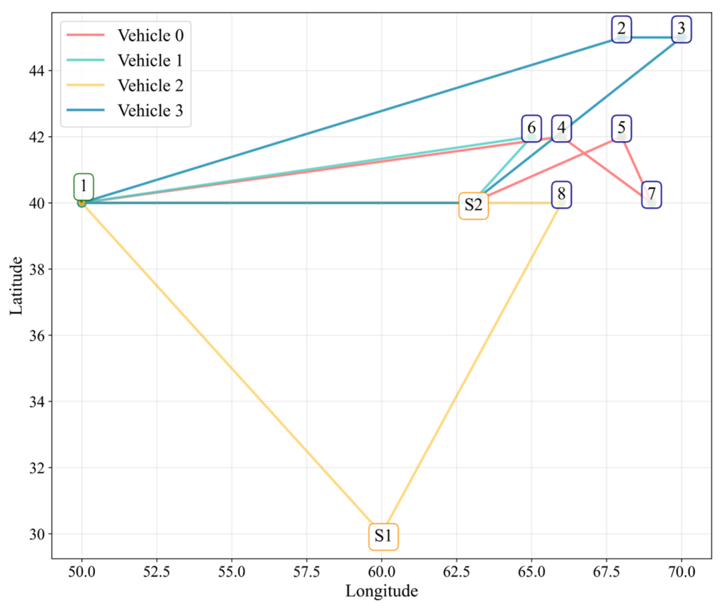
Given this convergence behavior, a gap smaller than 0.5% is taken as the stopping criterion for presenting the results, which demonstrates the reasonableness of the model’s output. At convergence, the total computational time was 60.3859 s, and four EVs were dispatched to serve the seven demand points. The route traveled by each EV in the network is shown in Figure 5.

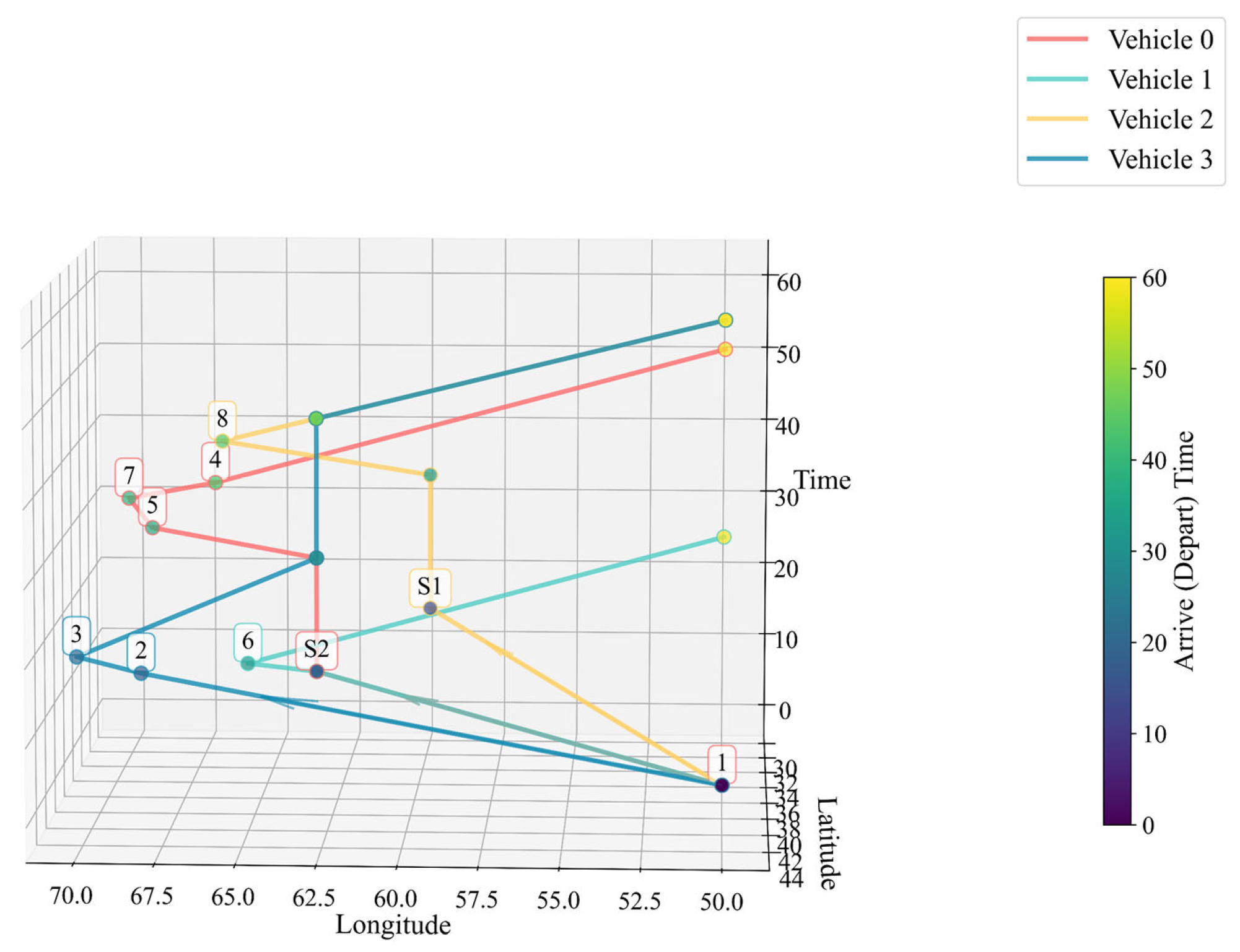
In Figure 5, all dispatched EVs start from the depot, serve their assigned demand points, and return to the depot, with every EV passing through S2 and Vehicle 2 additionally passing through S1. Since merely showing the routes does not convey the specific arrival/departure times at each node or adequately reflect the charger-quantity constraint considered in this study, namely, the limited number of EVs that can charge simultaneously at a CS, Figure 6 further displays the arrival and departure times of each EV at every node. If an EV charges or waits at a CS, it is depicted as not moving in geographical coordinates but progressing along the time axis.

It should be noted that the time units in the figures are directly calculated based on the parameter settings in Table 3, without any additional conversion. These parameter values are chosen to maintain consistency with Table 3, with the aim of focusing on demonstrating the effectiveness of the proposed model innovations.

As can be seen from Figure 6, Vehicle 1 passes through CS S2 without charging there, while all other EVs perform charging at CSs. Specifically, Vehicle 0 and Vehicle 3 both charge at S2. Vehicle 0 arrives first, completes charging, and departs before Vehicle 3 reaches S2, so no additional waiting time occurs. Meanwhile, to avoid potential waiting at S2, Vehicle 1 detours to S1 for charging. After serving customer node 8, it passes through S2 on its way back to the depot (without charging at S2, since S2 lies on the straight-line route from point 8 to the depot). Although the detour increases travel distance, it improves the overall task completion efficiency at the system level.

These results demonstrate that the model’s formulation of the charger-quantity constraint, i.e., the limit on the number of EVs that can charge simultaneously at the same CS, is reasonable and effective. Moreover, by optimizing the order in which EVs serve demand points and dynamically adjusting their routes, the model significantly reduces additional waiting time caused by competition for charging resources.

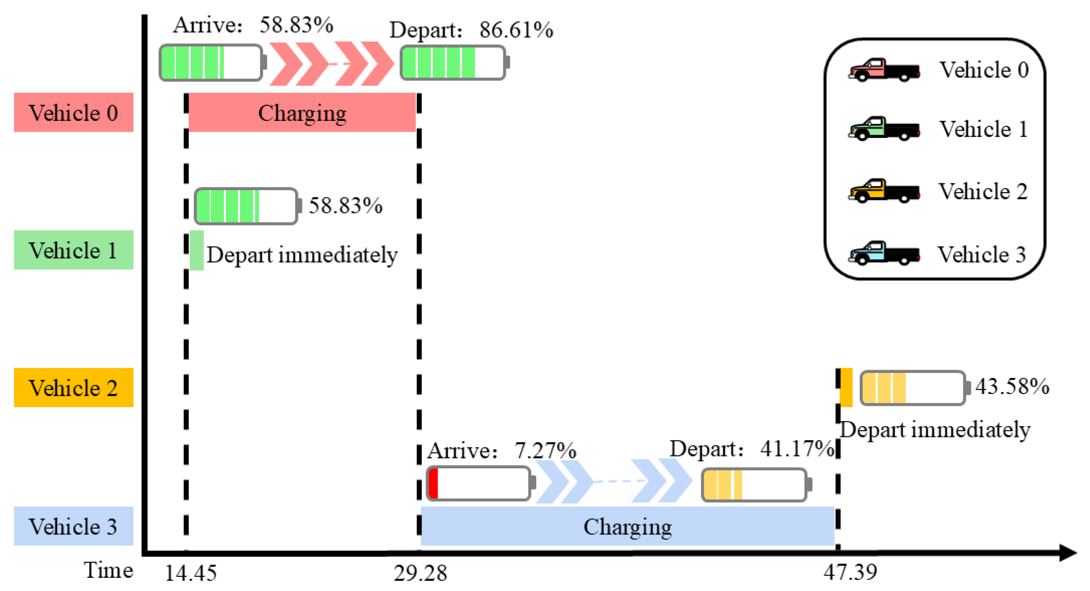
Because the details of waiting and charging behaviors, as well as battery SOC changes before and after charging, may not be fully visible in Figure 6, a more detailed view is provided in Figure 7 for CS S2, which is visited by multiple EVs. Figure 7 clearly displays the arrival time, charging duration, departure time, and battery SOC variation of every EV that passes through S2, offering a direct illustration of how the model effectively accounts for CS capacity constraints in vehicle dispatching and charging scheduling.

It should be noted that in the model, battery SOC is represented as absolute value, which makes it difficult to directly assess the reasonableness of charging behavior relative to the total battery capacity. Therefore, in Figure 7, the battery information of each EV is displayed as a percentage (i.e., the actual battery SOC divided by the maximum battery capacity B), enabling a more intuitive observation of energy changes.

From the arrival and departure times as well as the battery SOC variations before and after charging, it can be seen that when the number of chargers at CS S2 is set to 1 (i.e., capacity = 1), Vehicle 3, which goes to S2 for charging, arrives only after Vehicle 0 has finished charging. This again confirms the effectiveness of the CS capacity constraint formulated in this study.

Furthermore, if an EV charges upon arriving at a CS (as Vehicle 0 and Vehicle 3 do in Figure 7), the amount it charges depends on its actual route. Under the premise of optimizing the overall completion efficiency of all transportation tasks, the model does not force EVs to fully recharge at a CS; instead, it ensures that each EV has sufficient energy to return to the depot. Hence, from the perspective of overall system operational efficiency, the modeling approach proposed in this study can effectively utilize the chargers at CSs while avoiding unnecessary waiting time caused by excessive charging.

To verify that the proposed model can effectively utilize limited chargers and minimize waiting time by optimizing vehicle dispatching and charging strategies, it is compared with a common alternative approach. This benchmark approach typically enforces capacity constraints by limiting the total number of EVs arriving at a CS within predefined time periods. Accordingly, constraints (1) and (3)–(12) of the proposed model are simplified into the following form to serve as the comparative baseline.

$$\sum _{k\in \mathit{K}}\sum _{i\in \left\{i\left|\left(i,j\right)\in \mathit{E}\right.\right\}}{x}_{ij}^k⩽C_I.$$

(41)

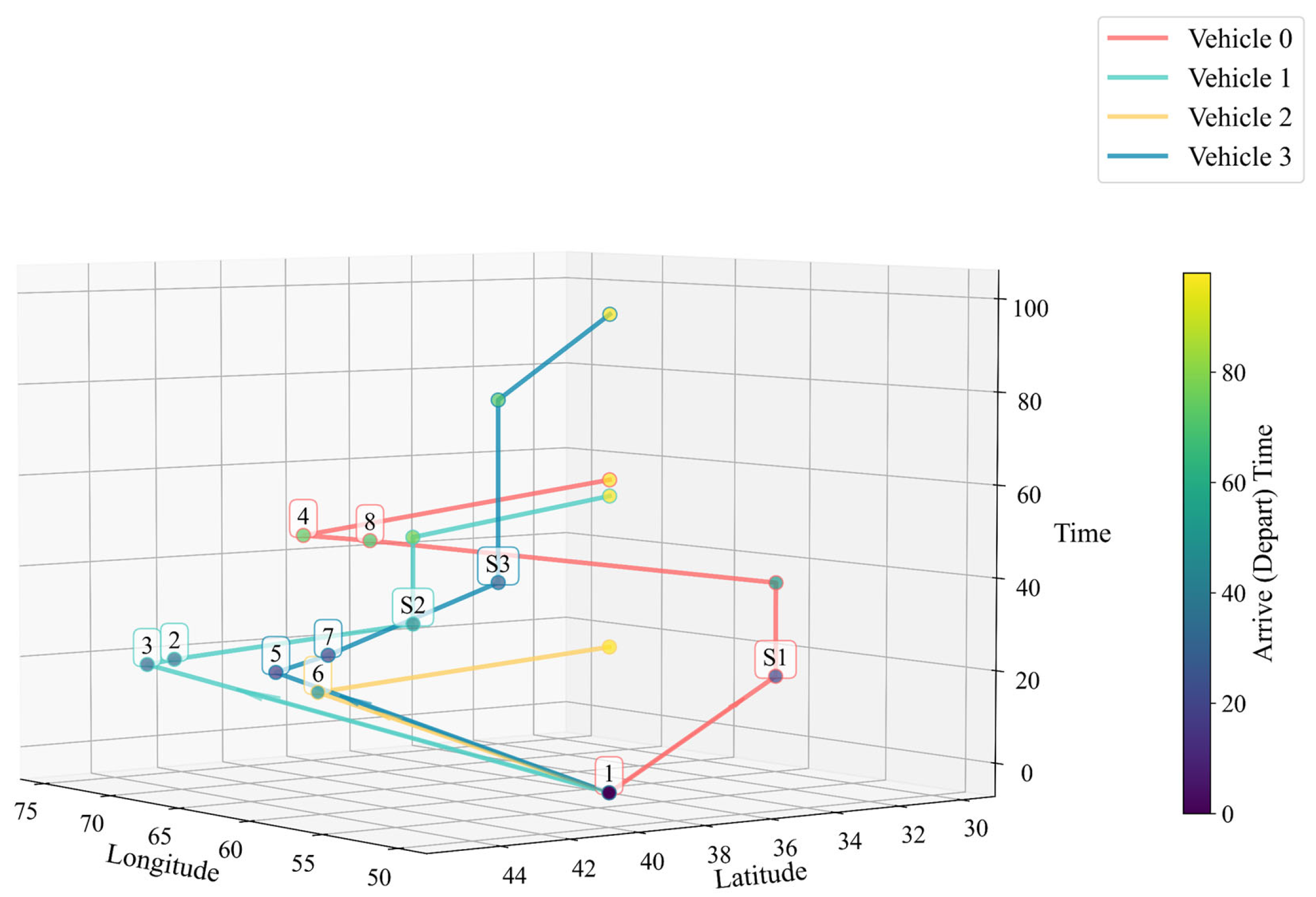
The comparison model was solved using the Gurobi solver, with the same input data (including the network structure and vehicle parameters of the test instance) as used for the main model. The resulting routes and timing information for all dispatched EVs are presented in Figure 8.

By comparing the results in Figure 8 with those in Figure 6, it can be observed that under the constraint which limits the total number of EVs allowed to arrive at a CS, EVs are often forced to detour to other CSs to recharge in order to meet their energy requirements. This strategy leads to a significant increase in the total task completion time at the system level: the objective value of the comparison model is 98.9, while that of the proposed main model is only 60.39, marking a notable improvement of approximately 38.9%.

This demonstrates that the CS capacity formulation proposed in this study can more fully utilize charging resources. It not only effectively reduces the waiting delay at a given CS but also avoids unnecessary time costs caused by excessive detours to alternative CSs, thereby further validating the rationality and superiority of the proposed capacity constraint modeling approach.

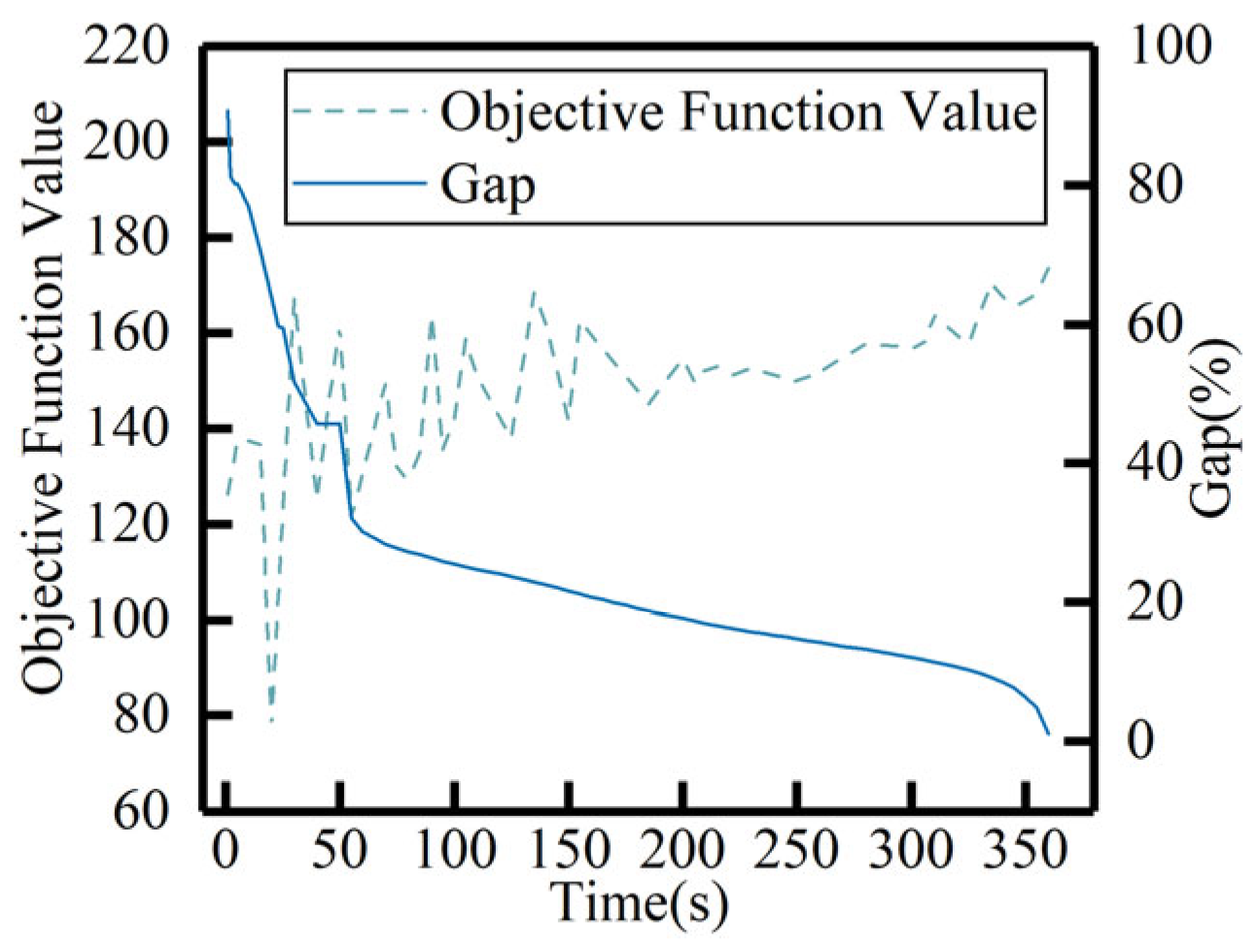
As mentioned above, in the small-scale instance, to demonstrate the effectiveness of the model constraints, we simplified the part of the objective function that controls the number of vehicles dispatched for transportation tasks. After incorporating this part into Gurobi to form the complete model, we solved it, and the evolution of the objective function value and the optimality gap during the solution process is shown in Figure 9.

As shown in Figure 9, in a transportation network with only eight customer nodes, Gurobi already requires approximately 360 s to converge, indicating a relatively slow solution speed. Therefore, when applying the proposed model to larger-scale networks, it is advisable to use the algorithm developed in this study. The following sections evaluate the performance of this algorithm.

To validate the solution accuracy of the algorithm, it should ideally be compared with the results obtained from Gurobi. However, given that Gurobi already takes considerable time to solve the network with eight customer nodes (plus one depot and three CSs), a further increase in network size would hinder the solution process. Hence, for the purpose of evaluating the algorithm’s optimality, we constructed a test network with 20 customer nodes. Specifically, 20 customer nodes were extracted from the C101 dataset to form the test network, while the locations of the three CSs and the number of chargers at each station remained unchanged.

Furthermore, the proposed algorithm incorporates a greedy criterion in its design phase, aiming to use as few vehicles as possible to complete the tasks. It does not dispatch excessive vehicles to accelerate task completion even when more vehicles are available. Accordingly, in the comparative experiments, we removed the vehicle-count control term from the objective function when solving with Gurobi, and set the number of available vehicles to be the same as that used in the algorithm for a fair comparison.

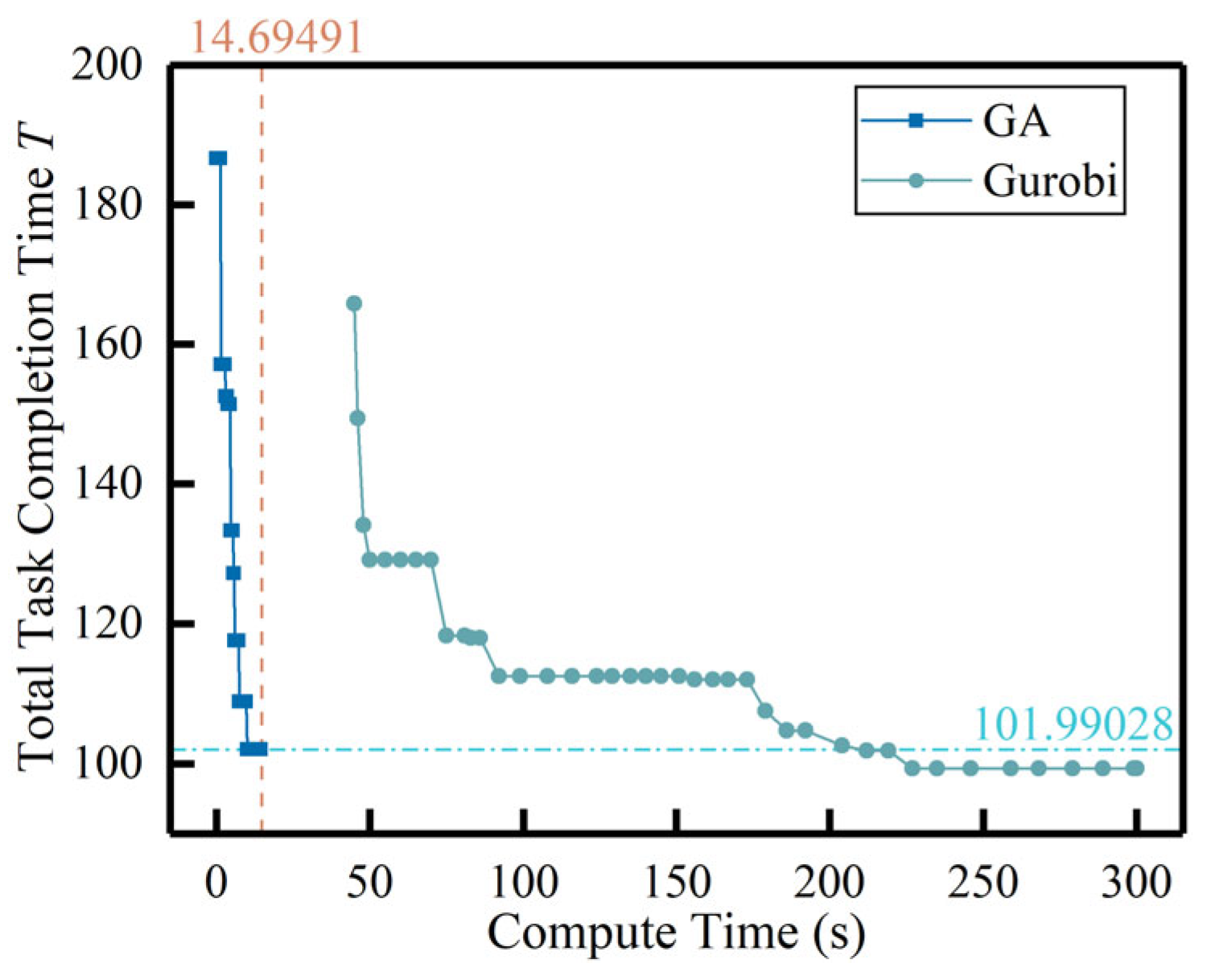
In addition to the above settings, the maximum number of EVs available in the transportation system is set to 6. For the GA, the probability of triggering Module 3 (p₁) is set to 0.5, and the probability of triggering Module 4 (p₂) is set to 0.95. The maximum number of iterations is set to 100, with early termination if the objective value does not improve for 20 consecutive iterations. Under these parameter settings, both the GA and Gurobi are used to solve the large-scale instance. The maximum runtime for Gurobi is limited to 300 s to simulate the high-timeliness requirements typical of real-world large-network scenarios. The evolution of the objective function over time for the two methods is shown in Figure 9.

As shown in Figure 10, the enhanced GA proposed in this study, built upon the classical genetic algorithm, obtains a high-quality solution (with a total task completion time T of approximately 101.99) for the same-scale problem as Gurobi in about 14.69 s, and converges rapidly. In contrast, although Gurobi finds a better solution (T≈99) after approximately 205 s, it fails to generate any feasible solution during the first 45 s (reflected by the blank segment of the Gurobi curve in the figure), and does not surpass the GA result until around 200 s. Notably, within the maximum time limit of 300 s, the optimal solution obtained by Gurobi is only about 2.9% better than that of the GA, while its runtime is approximately 185 s longer, about 13.3 times that of the GA. These results demonstrate that in time-sensitive application scenarios, the proposed enhanced GA can deliver acceptable-quality solutions with a minor loss in optimality, while requiring significantly less computational time, thereby validating its effectiveness in improving the solution efficiency of the model.

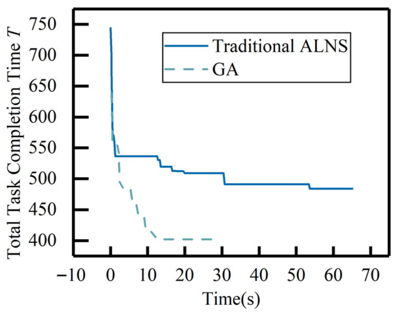
To evaluate the adaptability of the proposed algorithm to larger-scale networks, a medium-scale test network consisting of 60 customer nodes was extracted from the C101 dataset. The proposed algorithm was applied to solve this instance, and the adaptive large neighborhood search (ALNS) algorithm, commonly used for VRP variants, was adopted as a benchmark for comparison. It should be noted that the ALNS algorithm was not equipped with problem-specific operators tailored to the characteristics of our model. This is because the algorithmic modules developed in this study are themselves innovative designs addressing the specific features of the model; customizing ALNS with similar problem-specific operators would hinder a fair assessment of the effectiveness of our proposed algorithmic modules. The solution results of both algorithms are presented in Figure 11.

Figure 11 presents the performance of ALNS and the proposed GA under the same maximum number of iterations, where the GA terminates early if no improvement is observed for multiple consecutive iterations. As shown in the figure, the ALNS algorithm exhibits a faster initial descent than the proposed GA. However, benefiting from the problem-specific algorithmic modules designed for the model characteristics, the proposed GA achieves a steeper descent in subsequent iterations, after which it gradually stagnates and eventually terminates early due to lack of improvement. The GA completes its iteration in approximately 29 s with an objective value T of about 402, while ALNS maintains a steady descending trend throughout the process and completes computation in about 65.1 s with a T value of approximately 483.7. Overall, the proposed GA outperforms the conventional ALNS in both solution efficiency and quality.

It should be clarified that these results validate the effectiveness of the proposed GA but do not imply that GAs are inherently superior to ALNS. As mentioned earlier, the ALNS employed in the experiments is a conventional version designed for general VRP problems, without tailored destruction and repair operators customized for the specific characteristics of our model. Therefore, the performance difference reflects the degree of alignment between a general-purpose algorithm and the model’s features, rather than the inherent superiority of either algorithm.

It should be noted that the GA framework was chosen as the foundation of this study primarily due to considerations of implementation complexity. Designing problem-specific algorithmic modules within the GA framework is relatively straightforward and well-suited to the characteristics of the proposed model. However, the ALNS framework offers the potential for developing more efficient solution operators, albeit with higher implementation complexity. Based on the rapid descent characteristic of the proposed GA and the stable descending trend maintained by the conventional ALNS, it can be concluded that future research could leverage the strengths of the ALNS framework. By designing problem-specific operators based on the algorithmic modules developed in this study, more efficient solution methods could be explored within the ALNS paradigm, further improving solution efficiency and adaptability to larger-scale networks.

To analyze the sensitivity of the proposed model to parameter variations, this study adjusted the number of chargers at each CS and examined whether the computational results align with practical expectations. Specifically, the number of chargers C_I was set to 1, 2, and 3, respectively. Experiments were conducted on a test network with 60 customer nodes using the proposed GA, and the relationship between the total task completion time T and the number of chargers C_I is presented in

Table 4. Relationship between total task completion time and C_I.

Number of Chargers of Each CS	Total Task Completion Time
1	401.96
2	256.57
3	235.16

.

As shown in Table 4, the total task completion time T decreases significantly as the number of available chargers at each CS increases. This is because increasing the number of chargers enhances the station capacity in the proposed model, thereby reducing the waiting time incurred by EVs due to charger unavailability. Given that three CSs are configured in the test network, each increment of C_I by 1 effectively increases the total system capacity by three chargers.

Specifically, when C_I increases from 1 to 2, T drops markedly, indicating a substantial reduction in the number of EVs waiting due to capacity constraints. When C_I further increases from 2 to 3, T continues to decrease, but the downward trend slows considerably. This is because the number of EVs requiring waiting has already been largely mitigated at C_I = 2, leaving limited room for further improvement.

These results demonstrate that the proposed model is highly sensitive to the number of chargers at CSs, and can effectively capture the impact of CS capacity constraints on system performance.

6. Conclusions

This study proposes a novel optimization model that simultaneously considers CS capacity and electric vehicle battery capacity constraints. Through continuous-time modeling and a flexible charging decision mechanism, the model effectively captures vehicle waiting behavior under CS capacity limitations and allows EVs to autonomously determine charging amounts based on real-time status. To address the computational inefficiency of solving the model with Gurobi, an enhanced genetic algorithm is developed based on the classical GA framework, with problem-specific algorithmic modules designed to improve solution efficiency. Numerical results demonstrate that the model effectively reflects the impact of CS capacity constraints on system scheduling, and the proposed enhanced GA can efficiently solve a network with 60 customer nodes within 30 s, significantly improving the model’s adaptability and timeliness for practical applications. Furthermore, sensitivity analysis by varying the number of available chargers at each CS shows that the computational results respond effectively to capacity changes, further validating the effectiveness of the proposed model in handling CS capacity constraints.

Compared with existing studies that consider CS capacity limits, this model innovatively introduces a set of binary variables that formulate charging-decision constraints by comparing EV arrival and departure times, allowing EVs to autonomously decide when to charge. The approach neither employs discrete-time approximations nor imposes predefined charging amounts. This methodology offers two main advantages. First, the numerical results demonstrate that the proposed formulation can utilize limited charging resources more fully over the entire operational horizon, avoiding resource idleness that may arise from traditional discrete-time methods or from simply restricting the number of charging EVs. Second, the autonomous charging-decision mechanism in the model aligns better with real-world charging behavior, enabling EVs to reasonably pass through CSs to shorten routes, thereby preventing the loss of task-completion efficiency that could result from mandatory charging.

Despite the contributions of this study, several limitations should be acknowledged. First, the model assumes a linear relationship between charging duration and the amount of energy replenished, which may not fully capture the actual charging characteristics of electric vehicle batteries. Second, the model does not differentiate among various charging speeds and assumes that all chargers at CSs are identical, thereby overlooking the heterogeneity that may exist in real-world charging infrastructure. Third, the current model and algorithm are designed for static scenarios and cannot effectively accommodate dynamic factors such as real-time traffic fluctuations or unexpected charger failures. Although the proposed genetic algorithm aims to meet high timeliness requirements, it does not yet support real-time adjustments during route execution. Addressing these limitations by incorporating more accurate charging profiles, heterogeneous charger configurations, and dynamic response mechanisms constitutes important directions for future research.

Future work should address the aforementioned limitations through several directions. First, more accurate nonlinear charging profiles should be incorporated to better reflect the actual charging behavior of electric vehicle batteries. Second, heterogeneous charger configurations need to be considered to capture the diversity of real-world charging infrastructure. Third, dynamic response mechanisms should be developed to enable real-time route adjustments under fluctuating traffic conditions or unexpected charger failures. In addition, building upon existing studies, future research should further explore how to enhance task completion efficiency while ensuring resource utilization, thereby promoting the overall sustainability of logistics operations. These enhancements would align the model more closely with the practical requirements of real-world logistics scheduling and contribute to broader environmental goals.