Collaborative Optimization Scheduling of New Energy Vehicles and Integrated Energy Stations Based on Coupled Vehicle Routing and Charging Decisions

Abstract

To reduce charging time and improve operational efficiency at integrated energy stations (IESs) for electric vehicles (EVs), this paper develops a sustainability-oriented collaborative optimization model by coupling vehicle routing behavior with charging decision-making. Firstly, a dynamic road network model is established to simulate vehicle arrivals at IESs from different network nodes. Then, considering grid peak–valley electricity prices, station electricity procurement costs and EV charging demand, a dynamic pricing strategy for IESs is proposed to guide EVs to charge at off-peak hours so as to realize peak shaving and valley filling for the power grid. Meanwhile, the NSGA-III algorithm is improved through the introduction of Good Point Set initialization and an adaptive crossover mechanism, and the Good Point Set initialization and Adaptive Crossover NSGA-III (GPS-AC-NSGA-III) algorithm is proposed to solve the scheduling optimization problem. Finally, the CRITIC-based TOPSIS method is employed to identify the optimal compromise solution from the Pareto-optimal set. Case studies further prove the effectiveness of the proposed multi-objective collaborative optimization model for EVs and IESs. Compared with scenarios without dynamic Dijkstra-based navigation and dynamic pricing, the IES daily revenue increased by 39.83%, pollutant emissions decreased by 0.4%, and the peak-to-valley load difference ratio was reduced by 4.94%. The results indicate that dynamic Dijkstra-based vehicle routing improves travel efficiency, while the proposed dynamic pricing strategy enhances station profitability and smooths grid load fluctuations. Overall, the proposed framework contributes to sustainable transportation and energy systems by reducing pollutant emissions, improving energy efficiency, and enhancing the operational stability of integrated energy infrastructure, thereby supporting the transition toward low-carbon and sustainable urban energy systems.

1. Introduction

At present, China’s energy structure remains dominated by fossil fuels, and the carbon emission issues caused by their excessive consumption have become increasingly severe. To address the dual pressures of energy security and environmental protection, the government has actively promoted the development and large-scale deployment of renewable energy across various sectors [1,2]. In the automotive industry, new energy vehicles (NEVs) have emerged as a key development direction. According to data released by the National Bureau of Statistics, China’s NEV production reached 13.168 million units in 2024, representing a year-on-year increase of 38.7%. With the large-scale adoption of NEVs, the demand for vehicle charging and battery swapping has grown rapidly, and integrated energy stations (IESs) generally face shortages of charging infrastructure during peak electricity consumption periods [3]. Therefore, while improving vehicle routing efficiency and alleviating congestion in road networks, it is also necessary to further optimize the charging pricing mechanisms of IESs to mitigate the load pressure caused by concentrated charging during peak hours and to achieve peak shaving and valley filling.

To address peak-hour congestion and prolonged charging queue times, most existing studies have focused on optimizing EV routing strategies. Charging waiting times have been effectively reduced through improvements in pathfinding algorithms. For instance, Ref. [4] proposed a deep-reinforcement-learning-based EV charging navigation approach to minimize both travel time and charging costs. Ref. [5] established a stochastic traffic flow model to improve the accuracy of energy consumption prediction by capturing uncertainties such as travel time and vehicle speed, and further developed a cost-effective in-route charging navigation algorithm. Ref. [6] introduced a cost-based navigation method to identify charging stations with minimal total cost, thereby mitigating traffic congestion, where the target cost includes both temporal and monetary components. Ref. [7] developed a multi-criteria shortest path search algorithm based on a contracted hierarchy framework. In addition, Ref. [8] proposed a real-time EV charging navigation platform based on graph reinforcement learning, enabling continuous and adaptive route planning for multiple EVs. The aforementioned studies primarily concentrate on optimizing EV routing strategies, with relatively limited attention given to the role of charging stations in actively managing traffic flow. As key service providers in the charging process, charging stations can influence EV charging behavior through appropriate pricing mechanisms. Several studies have attempted to redirect EVs from congested charging stations to underutilized ones by adjusting charging prices among different stations [9,10,11,12], thereby reducing waiting times and alleviating congestion. However, existing research has rarely explored the implementation of time-varying pricing strategies at individual charging stations to incentivize EV charging during off-peak periods.

In recent years, increasing attention has been paid to renewable-energy-enabled EV charging systems, particularly photovoltaic (PV)-integrated and PV–storage coordinated charging stations. These systems aim to reduce carbon emissions and improve energy utilization efficiency by leveraging local renewable generation and energy storage technologies. Xiao, Y et al. [13] proposed a novel PV-ESS scheduling system integrating PV and energy storage systems (ESSs) to optimize electric bus charging. Xia, FZ et al. [14]. proposed a photovoltaic–storage fast charging station planning method considering charging demand response. The proposed method can effectively improve the profit of charging service providers and reduce the total charging time of EVs. In studies on charging station scheduling optimization, various innovative approaches, including reinforcement learning and adaptive control strategies, have been employed to improve operational performance [15,16,17,18]. In addition, several works have refined charging station modeling frameworks to enhance the accuracy of optimization scheduling [19,20]. These studies have improved the economic efficiency, operational stability, and environmental sustainability of charging stations by considering optimization objectives such as total operating cost, overall revenue, power fluctuations at grid connection points, carbon emissions, station capacity, and power quality. However, most existing research has primarily focused on individual charging stations, with limited attention given to the use of pricing strategies as a mechanism to guide EV charging behavior and achieve coordinated and optimized station operation.

With the rapid advancement of computational intelligence, evolutionary algorithms have been widely applied to multi-objective optimization problems in transportation and energy systems. Classical approaches include particle swarm optimization (PSO) and genetic algorithms (GAs), as well as their multi-objective extensions. For example, Akopov [21] proposed an improved parallel bi-objective real-coded genetic algorithm with clustering-based selection, demonstrating enhanced diversity preservation and convergence performance. Similarly, Leung et al. [22] developed a multi-objective PSO algorithm incorporating novel update strategies for improved solution quality. In terms of improving the initialization strategy of NSGA-III algorithm, Ma et al. [23] generated initial populations by integrating sampling techniques with the A* algorithm, effectively addressing issues associated with conventional random initialization strategies in vehicle routing planning, such as infeasible solutions and premature convergence to suboptimal scheduling schemes. Regarding non-dominated sorting enhancement, Zhang et al. [24] proposed an improved NSGA-III incorporating elimination strategies and a dynamic constraint relaxation mechanism, which strengthened selection pressure and improved constraint-handling capability. This approach effectively addressed complex constraints in integrated charging station scheduling and enabled the algorithm to approximate the feasible Pareto front more efficiently. Feng et al. [25] developed a two-stage individual feedback NSGA-III, which expanded global search capability and enhanced dynamic adaptability. In addition, several studies have integrated deep reinforcement learning with NSGA-III by embedding learning-based gene evolution mechanisms into the algorithmic framework. This hybrid approach enables the algorithm to extract scheduling knowledge from complex historical EV–station–network interaction data, thereby accelerating convergence toward high-quality solutions [26,27]. Methods such as MORCGA-MOPSO-II [21], MBHGA [28], and CBHPSO [29] combine the advantages of GA and PSO to balance global exploration and local exploitation. In the context of transportation system optimization, algorithms including fuzzy clustering-based genetic algorithms (FCGAs) [30], BORCGA-BOPSO [31], and MA-HCAGA [32] have also been applied to complex multi-objective problems, showing strong performance in handling nonlinearity and uncertainty. Despite these advances, most existing algorithms still exhibit limited search efficiency when tackling highly complex multi-objective optimization problems. Further research is required to strengthen local search capability and improve convergence performance.

Therefore, to enhance EV charging efficiency and optimize the operational performance of charging stations, this paper investigates the interaction between EV charging decisions and charging station electricity pricing. A dynamic pricing strategy is formulated, and an optimal scheduling framework for IESs is developed based on vehicle traffic data. The main contributions of this paper are summarized as follows:

(1)

A collaborative optimization model for EVs and integrated energy stations is established. Unlike conventional studies that treat EV routing and charging station operation separately, this paper explicitly models the coupling between EV routing decisions and charging station operational optimization. By integrating traffic dynamics into the decision-making process, the proposed framework enables coordinated optimization of user-side behavior and station-side energy management.

(2)

A dynamic pricing strategy for IESs is proposed. The proposed pricing strategy considers time-of-use electricity prices, station procurement costs, and EV charging demand. It serves as a coordination signal to guide EV charging behavior and improve load distribution, thereby facilitating peak shaving and valley filling.

(3)

An improved multi-objective optimization algorithm, GPS-AC-NSGA-III, is developed. By incorporating Good Point Set initialization, adaptive crossover, and Cauchy mutation into NSGA-III, the proposed algorithm enhances population diversity and convergence performance, ensuring effective solution of the complex coupled optimization problem.

(4)

The proposed optimization framework is validated through comprehensive case studies. Using GPS-AC-NSGA-III to solve the collaborative optimization problem. The results demonstrate that the proposed method improves economic performance, reduces emissions, and enhances load stability compared with baseline approaches.

2. Mathematical Model

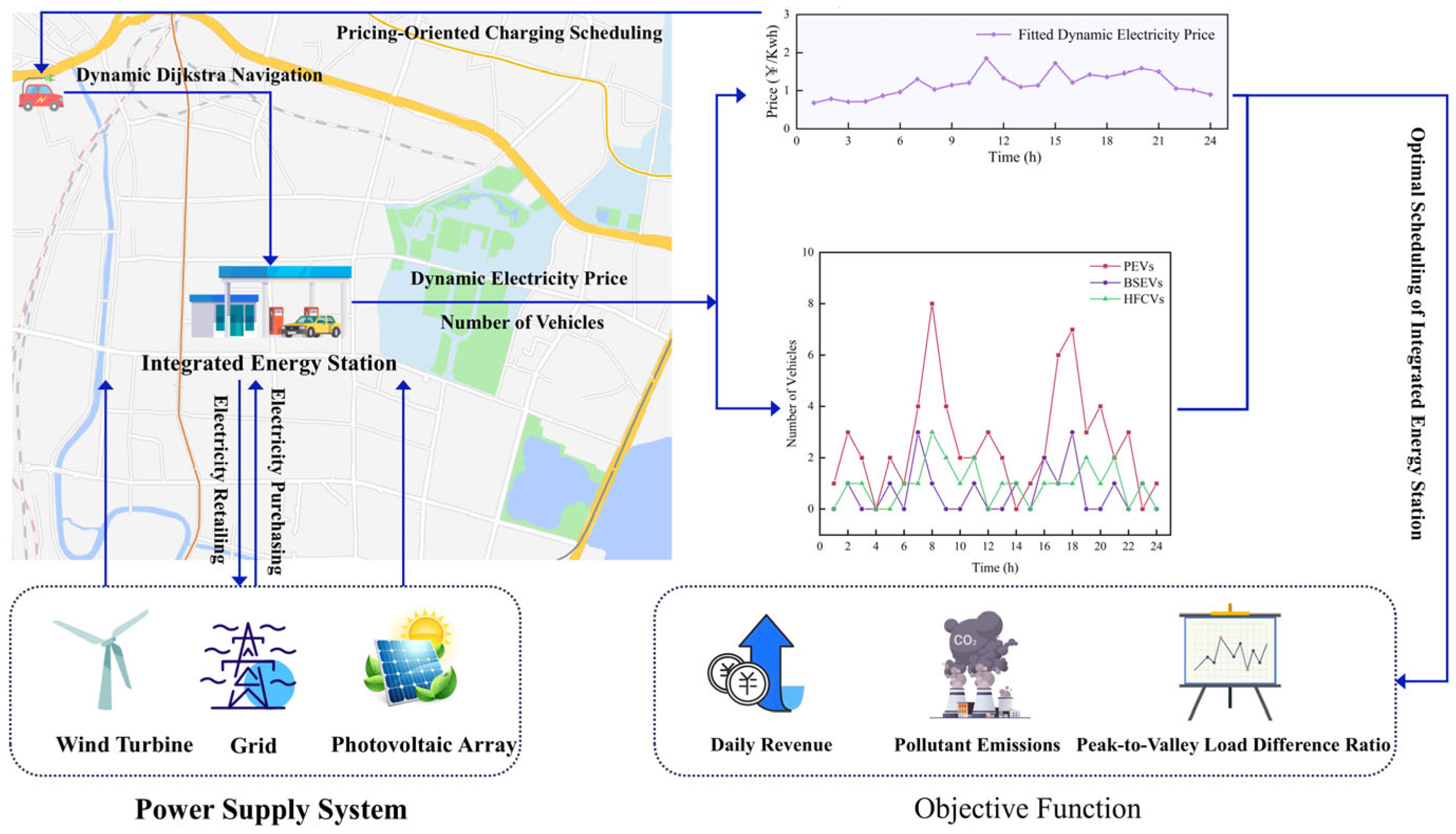
The IES optimization framework developed in this study, based on the coupling of vehicle pathfinding and charging behaviors, is illustrated in Figure 1. The operational process of the proposed framework is described as follows. First, based on the road network topology, the Monte Carlo method is employed to simulate and generate the travel trajectories and charging demands of EVs. Subsequently, a dynamic Dijkstra algorithm is applied to perform real-time path planning by minimizing travel time costs, thereby guiding EVs with charging demand to the optimal IES. The IES integrates wind power and photovoltaic generation systems to enhance energy self-sufficiency. Its operational model allows electricity to be purchased from the power grid during periods of insufficient renewable generation and surplus electricity to be sold back to the grid to obtain economic benefits. Furthermore, by introducing a dynamic pricing mechanism, the IES can actively regulate the temporal distribution of EV arrivals across different time periods. This coordinated strategy enables the simultaneous optimization of three key objectives: daily operational revenue, carbon emissions, and the grid-side peak-to-valley load difference ratio.

2.1. Dynamic Traffic Road Network Model

The traffic road network model in this study is formulated based on graph theory. Compared with microscopic or mesoscopic traffic models that explicitly simulate individual vehicle interactions, this modeling choice is motivated by several considerations. First, the primary objective of this study is to investigate the system-level interaction between EV routing decisions and charging station operation, rather than to reproduce detailed vehicle maneuvering dynamics. Second, incorporating microscopic traffic behavior would significantly increase computational complexity, making it difficult to integrate with large-scale multi-objective optimization. Third, graph-based models with time-dependent travel times have been widely used in dynamic routing problems and can effectively approximate aggregate traffic conditions. The topological structure is mathematically represented as shown in Equation (1):

$$\left\{\begin{array}{l}G=(V,E,K,W)\hfill \\ V=\left\{v_i|i=1,2,3,\dots ,n\right\}\hfill \\ E=\left\{v_{ij}|v_i\in V,v_j\in V,i\ne j\right\}\hfill \\ K=\left\{k|k=1,2,3,\dots ,m\right\}\hfill \\ W=\left\{w_{ij}^k|v_{ij}\in E,k\in K\right\}\hfill \end{array}\right.$$

(1)

The road network topology is represented by $G(V,E,K,W)$, where V denotes the set of nodes, E indicates the set of edges within the network, K represents the set of discrete time periods, and W signifies the set of roadway weights.

A dynamic traffic road network model is employed in this study to simulate vehicle travel. In contrast to the traditional Dijkstra [33] algorithm used for determining the shortest path between origin–destination (OD) pairs, the dynamic Dijkstra algorithm is capable of identifying the route with the minimum travel time. The roadway weights, denoted by W, represent the travel cost along road segments and are quantified using parameters such as roadway length, travel speed, travel time, and travel cost. In urban road networks, intersections are typically controlled by traffic signals, and vehicle travel is influenced by both Link impedance and delays at intersections. Therefore, the urban roadway resistance model is formulated as shown in Equation (2):

$$W_{ij}^k(t)=R{v}_{ij}(t)+C{v}_i(t)$$

(2)

where $R{v}_{ij}(t)$ represents the link impedance model, while $C{v}_i(t)$ corresponds to the node impedance model.

According to China’s urban traffic condition classification standard, traffic saturation [34] is evaluated using indices for smooth flow ($0<S\le 0.6$), moderate congestion ($0.6<S\le 0.8$), and severe congestion ($1.0<S\le 2.0$). Road intersections and segments exhibit varying traffic capacities, and the corresponding link and node impedance models can be derived based on the saturation level.

(1)

Link Impedance Model

$$R{v}_{ij}(t)=\left\{\begin{array}{ll}{R}^1{v}_{ij}(t):t_0(1+\alpha {(S)}^{\beta }),& 0<S\le 1.0\hfill \\ R^2{v}_{ij}(t):t_0(1+\alpha {(2-S)}^{\beta }),& 1.0<S\le 2.0\hfill \end{array}\right.$$

(3)

where $S={\displaystyle \frac{Q}{C}}$ represents the saturation level, Q denotes the roadway traffic flow, C is the roadway capacity, $t_0$ refers to the zero-flow travel time, and α and β are the impedance impact factors.

(2)

Node Impedance Model

$$C{\nu }_i(t)=\left\{\begin{array}{ll}{C}^1{\nu }_i(t):{\displaystyle \frac{9}{10}}\left[{\displaystyle \frac{c{(1-{\lambda }_g)}^2}{2(1-{\lambda }_{g}S)}}+{\displaystyle \frac{S^2}{2q(1-S)}}\right],\hfill & 0<S\le 0.6\hfill \\ C^2{\nu }_i(t):{\displaystyle \frac{c{(1-{\lambda }_g)}^2}{2(1-{\lambda }_{g}S)}}+{\displaystyle \frac{1.5(S-0.6)}{1-S}}S,\hfill & S>0.6\hfill \end{array}\right.$$

(4)

where c denotes the signal cycle duration, ${\lambda }_g$ represents the green time ratio, and q indicates the vehicle arrival rate on the road section.

The roadway impedance model presented in Equation (5) is derived by combining the link impedance model with the node impedance model:

$$w_{ij}(t)=\left\{\begin{array}{ll}{R}^1{\nu }_{ij}(t)+C^1{\nu }_i(t),\hfill & 0<S\le 0.6\hfill \\ R^1{\nu }_{ij}(t)+C^2{\nu }_i(t),\hfill & 0.6<S\le 0.8\hfill \\ R^2{\nu }_{ij}(t)+C^1{\nu }_i(t),\hfill & 0.8<S\le 1.0\hfill \\ R^2{\nu }_{ij}(t)+C^2{\nu }_i(t),\hfill & 1.0<S\le 2.0\hfill \end{array}\right.$$

(5)

2.2. Vehicular Mobility Model

The travel characteristics of EVs and hydrogen fuel cell vehicles (HFCVs) are analyzed in this study. EVs visit charging stations to recharge or replace batteries when a charging demand arises. HFCVs generate electricity through the electrochemical reaction between hydrogen and oxygen in a fuel cell, which powers an electric motor to propel the vehicle. The hydrogen refueling process resembles that of conventional fuel vehicles, such that refueling time can be considered negligible.

2.2.1. Automotive Travel Data

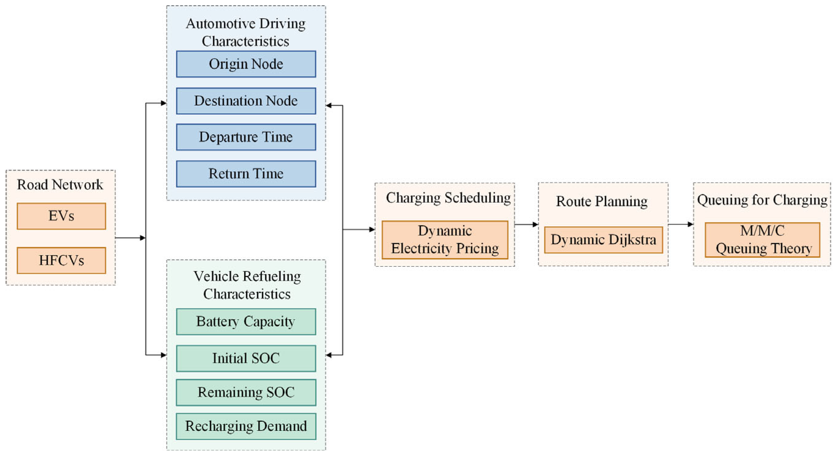
The Monte Carlo algorithm [35] is a computer-based stochastic simulation method grounded in probability and statistical theory, which enables more realistic representation of system behaviors and physical experimental processes. In this study, for each type of NEV, vehicle driving data was randomly sampled, and an origin–destination (OD) start–stop matrix method was introduced to simulate vehicle travel behavior. The corresponding load demand was then calculated. The start–stop matrix was constructed based on the variation in traffic flow across different time periods on each road segment, and the Monte Carlo sampling method was applied to assign each vehicle’s travel origin and destination, initial departure time, and return time. The parameter settings for the Monte Carlo simulation and the OD pair extraction parameters are presented in

Table 1. Parameter Settings for Monte Carlo Simulation.

Monte Carlo Simulation Variable	Distribution Type	Parameter
OD Pair	Random Sampling	NOD = 1000
Initial EV SOC	Normal Distribution	N (0.5, 0.1)
EV Travel Speed	Normal Distribution	N (30, 1)
EV Battery Capacity	Gamma Distribution	α = 10.08, β = 0.8
Road Segment Saturation S	Uniform Distribution	U (0, 2)

. The vehicle charging process is illustrated in Figure 2, and the OD start-stop probability matrix is provided in Equation (6):

$$C_{ij}={\displaystyle \frac{b_{ij}}{{\displaystyle \sum _{j=1}^n{b}_{ij}}}},\hspace{1em}(1\le i\le n, 1\le j\le n, i\ne j)$$

(6)

where $b_{ij}$ denotes the vehicle traffic volume between origin node i and destination node j during time period T; $C_{ij}$ represents the probability distribution of travel initiation times between nodes i and j [36]. To identify the optimal travel path between OD pairs, the dynamic Dijkstra algorithm is employed to guide routing based on the minimum travel time criterion.

2.2.2. EV Charging Conditions

The initial state of charge (SOC) of EVs is assumed to follow a normal distribution, and the initial available energy $C_0(i)$ is calculated based on the battery capacity of the EV. To minimize battery degradation due to overcharging, the maximum charging limit is set to 90% of the total battery capacity. The power consumption per kilometer is assumed to increase linearly with mileage, and the remaining power $C_t(i)$ at time t is expressed by Equation (7):

$$C_t(i)={\eta }_c(C_{t-1}(i)-\Delta l\cdot E_c)$$

(7)

where ${\eta }_c$ is the energy consumption coefficient, $E_c$ denotes the power consumption per kilometer, $C_t(i)$ is the remaining power at time t, and $\Delta l$ is the distance traveled by the ith vehicle from time t − 1 to time t.

Based on the remaining SOC of EVs and the electricity price at the charging station, the trigger conditions for EV charging and battery swapping defined in this study are provided in Equations (8) and (9):

$$Ch(i)=(C_t(i)\le C_{th1})\vee [(p_c(t)\le p_{c,th})\wedge (C_t(i)\le C_{th2})]$$

(8)

$$Bs(i)=(C_t(i)\le C_{th3})\vee [(p_c(t)\le p_{c,th})\wedge (C_t(i)\le C_{th4})]$$

(9)

where $Ch(i)$ and $Bs(i)$ represent the trigger conditions for EV charging and battery swapping behaviors, respectively. $C_{th1}$ and $C_{th3}$ denote the power thresholds required to initiate charging and battery swapping under normal conditions, while $C_{th2}$ and $C_{th4}$ indicate the adjusted thresholds for charging and swapping once the station tariff $p_c(t)$ exceeds a predefined tariff threshold $p_{c,th}$.

2.2.3. Modeling User Choice Behavior for Charging Stations

To rigorously characterize the interaction between EV travel behavior and charging station operations, this study considers a multi-station scenario. EV users can choose from multiple charging stations located at different geographical sites with varying charging prices. In the process of trip decision-making, drivers typically select their routes based on a subjective evaluation of travel utility, which is often influenced by multiple factors, including travel time and charging price. Assuming that user n faces a set of K available charging stations at time t, the observable utility function for user n choosing station k is expressed as shown in Equation (10), and the probability of selecting station k follows a multinomial logit formulation, as presented in Equation (11):

$$U_n^k={\beta }_t\cdot T_{travel}+{\beta }_p\cdot p_c(t)+{\beta }_w\cdot T_{wait}$$

(10)

$$P_{n,k}={\displaystyle \frac{\exp (U_n^k)}{{\displaystyle \sum _{j\in K}\exp }(U_n^j)}}$$

(11)

where ${\beta }_t$ is the travel time coefficient, set to −0.15, $T_{travel}$ is the travel time; ${\beta }_p$ is the charging price coefficient, set to −0.08; $p_c(t)$ is the charging price; ${\beta }_w$ is the waiting time coefficient, set to −0.12 [37]; and $T_{wait}$ is the queuing time. This paper establishes a closed-loop interaction mechanism between EV route planning and charging station operations. Charging prices and station congestion levels influence users’ route planning decisions, and the total charging demand generated by these decisions subsequently affects the operations, revenue, and queuing dynamics of the charging stations.

2.3. Integrated Energy Station Model

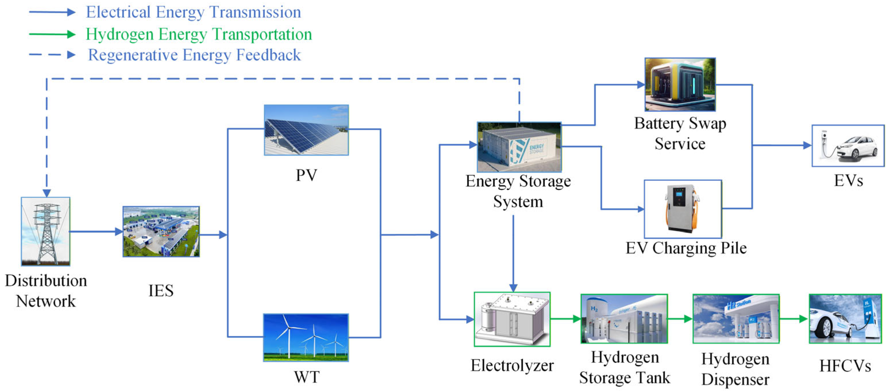
IES offer convenient and efficient charging and swapping services for NEVs. In this study, a model for an IES is proposed, which accommodates both the charging requirements of EVs and the hydrogen refueling needs of HFCVs [38]. The model is capable of purchasing electricity from or selling it to the grid to satisfy vehicle energy demands and enhance station profitability.

The overall structure of the model is illustrated in Figure 3. The IES comprises an external power grid, a wind power generation system, an energy storage system, and a hydrogen production unit. Power can be purchased from the external grid or generated via the wind system to supply the station. Surplus energy can be fed back to the grid, contributing to peak shaving and valley filling while significantly enhancing station profitability. The station intelligently allocates power between the energy storage system and the hydrogen production unit. Additionally, the energy storage system can support hydrogen production, thereby improving overall system economy and flexibility. The energy storage system manages the battery charging and discharging processes and oversees battery distribution, with a portion designated for EV battery swapping services. In the hydrogen production process, electricity is supplied to an electrolyzer to produce hydrogen via water electrolysis. The generated hydrogen is then compressed and stored in a hydrogen tank using an appropriate storage method.

2.3.1. Photovoltaic Model

Photovoltaic (PV) power generation refers to the process of converting solar energy into electricity through the photovoltaic effect. Photons from sunlight are absorbed by the photosensitive materials in PV panels, exciting electrons and thereby generating an electric current [39].

$$P_{PV}(t)={\displaystyle \frac{G_c(t)}{G_r}}\times P_{rp-PV}\times {\eta }_{PV}\times \left[1+k(T_c(t)-T_{rc})\right]$$

(12)

where $P_{PV}(t)$ represents the PV output power during time period t, $G_c(t)$ denotes the solar irradiance during time period t, $G_r$ refers to the rated solar irradiance under standard test conditions, $P_{rp-PV}$ is the rated output power of the PV panels under standard irradiance and temperature, ${\eta }_{PV}$ indicates the power conversion efficiency of the PV panels, $T_c(t)$ represents the ambient temperature during time period t, $T_{rc}$ is the reference temperature under standard conditions, and k denotes the power temperature coefficient of the PV panels.

2.3.2. Wind Power Model

Wind power refers to the conversion of kinetic energy from wind into electricity, which serves as a clean and renewable energy source capable of reducing dependence on conventional fossil fuels and minimizing adverse environmental impacts. The following formula estimates the electricity generated by wind turbines at the IES [40]:

$$P_{WT}=\left\{\begin{array}{l}0\\ {\displaystyle \frac{P_R}{(V_R^3-V_{ci}^3)}}\cdot V_t^3-{\displaystyle \frac{V_{ci}^3}{(V_R^3-V_{ci}^3)}}\cdot P_R\\ P_R\\ 0\end{array}\right.$$

(13)

where $V_t$, $V_R$, $V_{ci}$ and $V_{co}$ represent the actual wind speed, rated wind speed, cut-in wind speed, and cut-out wind speed, respectively, measured at the hub height of the turbine, and $P_R$ denotes the rated power output of the turbine.

2.3.3. Energy Storage Model

The energy storage system constitutes a critical component of the IES and is functionally divided into a charging station and a battery swapping station.

(1)

Battery Charging Station

In this study, the power value of the charging system is considered positive during the charging process and negative when discharging. The charging and discharging behavior of the battery system is represented by Equation (14) [41]:

$$SO{C}_{BCS}(t)={\displaystyle \frac{E_{BCS}(t-1)+P_{ch}(t)\cdot {\eta }_{ch}\cdot \Delta t_1-P_{dis}(t)\cdot {\eta }_{dis}\cdot \Delta t_2}{C_{BCS}}}$$

(14)

where $SO{C}_{BCS}(t)$ denotes the SOC at the charging station at time t; $E_{BCS}(t-1)$ represents the SOC at time t − 1; $P_{ch}(t)$ and ${\eta }_{ch}$ represent the charging power and charging efficiency at time t, respectively; $P_{dis}(t)$ and ${\eta }_{dis}$ denote the discharging power and discharging efficiency at time t, respectively; $\Delta t_1$ and $\Delta t_2$ correspond to the charging duration and discharging duration of the battery; and $C_{BCS}$ refers to the total capacity of the battery charging system.

(2)

Battery Swapping Station

When an EV arrives at the battery swapping station, its depleted battery is replaced with a fully charged battery, and the removed battery is subsequently recharged [42]. The number of fully charged batteries is denoted by $N_{ESB}$, and the model of the battery swapping station is illustrated below:

$$\left\{\begin{array}{l}{N}_{BSS}(t) =N_{BSS}(t-1)-N_s(t-1)\\ W_{BSS}(t)={\displaystyle \sum _{n=1}^{N_s}\left[\left(0.9-SO{C}_{BSEV}^{t-1}(n)\right)\cdot C_{EV}\right]}\end{array}\right.$$

(15)

where $N_{BSS}\left(t\right)$ represents the number of fully charged batteries at time t; $N_s(t-1)$ denotes the number of EVs that underwent battery swapping at time t − 1; $W_{BSS}(t)$ indicates the total amount of electricity consumed to recharge depleted batteries after vehicle swapping; $SO{C}_{BSEV}^{t-1}(n)$ is the SOC of the battery in the nth vehicle upon arrival at the swapping station at time t − 1; and $C_{EV}$ denotes the capacity of a single battery.

2.3.4. Hydrogen Production Model

The hydrogen production system primarily supplies hydrogen for refueling HFCVs and manages hydrogen production and storage based on a defined scheduling strategy and the storage tank’s capacity. This ensures that the hydrogen supply satisfies vehicle demand without exceeding the tank’s storage limits. Hydrogen stored in the tank is delivered to HFCVs via the hydrogen refueling module to support vehicle operation.

(1)

Electrolyzer Model

Hydrogen generation is achieved via water electrolysis employing an electrolyzer, with the electrochemical reaction detailed in Equation (16). The polymer electrolyte membrane (PEM) electrolyzer, characterized by its compact structure and low-temperature operation, enables the efficient production of high-purity hydrogen at pressures reaching up to 200 bar [43]. The conversion model for hydrogen production via PEM water electrolysis is provided in Equation (17):

$$H_{2}O+Electricity\to H_2+{\displaystyle \frac{1}{2}}{O}_2$$

(16)

$$P_t^E={\displaystyle \frac{(m_t^E\cdot LH{V}_{H_2})}{{\eta }_E}}$$

(17)

where ${\eta }_E$ denotes the efficiency of the electrolyzer, $m_t^E$ is the hydrogen mass flow rate at the electrolyzer outlet, $LH{V}_{H_2}$ represents the lower heating value (LHV) of hydrogen, and $P_t^E$ refers to the power consumed by the electrolyzer at time t.

(2)

Compressor Model

A compressor functions as a mechanical apparatus for increasing the pressure of gases or vapors [44], and plays an integral role in the hydrogen electrolysis system. Its energy supply is sourced from a photovoltaic system, wind power, energy storage units, and the external power grid. The operational characteristics of the compressor are formulated in Equation (18):

$$P_t^{comp}=C_{comp}\cdot {\displaystyle \frac{(T_{in}\cdot {10}^4)}{({\eta }_{motor}\cdot {\eta }_{comp}\cdot \Delta t)}}\left({\left({\displaystyle \frac{p_{out}^{comp}}{p_{in}^{comp}}}\right)}^{({\displaystyle \frac{r-1}{r}})}-1\right)\cdot ({\displaystyle \frac{m_t^E}{3600}})$$

(18)

where $C_{comp}$ represents the specific heat capacity of hydrogen at constant pressure, $P_t^{comp}$ denotes the power consumed by the compressor motor at time t, $p_{in}^{comp}$ and $p_{out}^{comp}$ correspond to the inlet and outlet pressures of the compressor, respectively, and r denotes the specific heat ratio of hydrogen. $T_{in}$ is the temperature of hydrogen at the compressor inlet, ${\eta }_{comp}$ is the isentropic efficiency of the compressor, and ${\eta }_{motor}$ represents its mechanical efficiency. The specific parameter values used in the compressor model are listed in

Table 2. Specific parameters used in the compressor model.

Parameters	${\mathit{C}}_{\mathit{c}\mathit{o}\mathit{m}\mathit{p}}$	${\mathit{T}}_{\mathit{i}\mathit{n}}$	${\mathit{\eta }}_{\mathit{c}\mathit{o}\mathit{m}\mathit{p}}$	${\mathit{p}}_{\mathit{i}\mathit{n}}^{\mathit{c}\mathit{o}\mathit{m}\mathit{p}}$	${\mathit{p}}_{\mathit{o}\mathit{u}\mathit{t}}^{\mathit{c}\mathit{o}\mathit{m}\mathit{p}}$
Value	14.304 kJ/kg	293 K	70%	1 MPa	90 MPa

.

3. Multi-Objective Optimization Problem Formulation

3.1. Objective Function

In the IES model developed in this study, three objective functions are formulated: namely, the daily revenue of the station, the pollutant emissions, and the peak-to-valley load difference ratio.

3.1.1. Daily Revenue

From an operational perspective, the total profit $F_1$ of the IES serves as a primary objective, which is composed of the revenue $F_{BES}$ from the energy storage system and revenue $F_{HPS}$ from the hydrogen production system. Dynamic pricing-based energy management between EVs and the power grid enhances overall operational efficiency. In this study, the optimization algorithm is designed to minimize the objective function; thus, the profit objective function is expressed as a negative value in the code to align with the minimization requirement.

$$F_1=F_{BES}+F_{HPS}$$

(19)

$$\begin{array}{ll}{F}_{BESS}=& {\displaystyle \sum _{t=1}^{24}{P}_{GES}(t)\cdot \Delta t\cdot p_{GES}(t)+{\displaystyle \sum _{t=1}^{24}{\displaystyle \sum _{n=1}^{N_c}{C}_{EV}\cdot (0.9-SO{C}_{BCEV}(n))\cdot p_c(t)}}}\\ & +{\displaystyle \sum _{t=1}^{24}{\displaystyle \sum _{n=1}^{N_s}{C}_{EV}\cdot (0.9-SO{C}_{BSEV}(n))\cdot p_c(t)}-{\displaystyle \sum _{t=1}^{24}{P}_{GEP}(t)\cdot \Delta t\cdot p_{GEP}(t)}}\end{array}$$

(20)

$$F_{HPS}={\displaystyle \sum _{t=1}^{24}{\displaystyle \sum _{n=1}^{N_f}\left(1-SO{C}_{FCEV}(n)\right)\cdot C_{FCEV}\cdot p_{HE}}}$$

(21)

where the power sold to and purchased from the grid by the charging station at time t are denoted by $P_{GES}(t)$ and $P_{GEP}(t)$, respectively. $p_{GES}(t)$ represents the electricity selling price to the grid at time t, while $p_c(t)$ denotes the charging and battery swapping price for EVs at the same time. $p_{GEP}(t)$ is the electricity purchasing price from the grid, and $p_{HE}$ denotes the hydrogen refueling price for HFCVs. $N_c$, $N_s$, and $N_f$ represent the total numbers of EVs arriving at the station for charging, battery swapping, and hydrogen refueling at time t, respectively. $C_{EV}$ denotes the battery capacity of EVs, and $C_{FCEV}$ represents the hydrogen capacity of HFCVs. $SO{C}_{BCEV}(n)$ and $SO{C}_{BSEV}(n)$ indicate the battery states of EVs requiring charging and swapping, respectively, while $SO{C}_{FCEV}(n)$ denotes the hydrogen status of vehicles requiring refueling.

3.1.2. Pollutant Emissions

With the increasing penetration of renewable energy, global carbon emissions are expected to gradually decline. The carbon emissions associated with clean energy sources, such as wind power and photovoltaic generation, are nearly negligible [45]. Therefore, environmental pollutant emissions mainly stem from the electricity purchased by integrated energy stations (IESs) from the public power grid. Accordingly, the minimization of pollutant emissions is formulated as the second objective function, as described in Equation (22):

$$F_2={\displaystyle \sum _{t=1}^{24}(e_1+e_2+e_3)\cdot P_{GEP}(t)\cdot }\Delta t$$

(22)

where $e_1$, $e_2$, and $e_3$ represent the emission factors for $C{O}_2$, $S{O}_2$, and $N{O}_x$, respectively, where $e_1=0.997 kg/kWh$, $e_2=0.03 kg/kWh$, and $e_3=0.015 kg/kWh$ [46]; $\Delta t$ denotes the charging time; and $P_{GEP}(t)$ is the power drawn from the grid by the charging station at time t.

3.1.3. Peak-To-Valley Load Difference Ratio

As a distributed energy storage node, the battery energy storage system (BESS) exerts a notable impact on the load dynamics of the regional power grid through its charging and discharging behaviors. Consequently, implementing optimized scheduling and coordinated control of these processes contributes to peak shaving and valley filling, thereby improving the operational reliability and overall stability of the power network. The Peak-to-Valley Load Difference Ratio, which quantitatively captures load fluctuation characteristics on the grid side, is computed as follows:

$$P_{load}=(P_{load}(1),P_{load}(2),P_{load}(3),\cdot \cdot \cdot ,P_{load}(24))$$

(23)

This study formulates an objective function aimed at minimizing the Peak-to-Valley Load Difference Ratio on the grid side, as expressed in Equation (24):

$$F_3={\displaystyle \frac{(P_{peak}-P_{valley})}{P_{peak}}}$$

(24)

where $P_{peak}$ represents the grid load during the peak period at the IES, i.e., $P_{peak}=\max (P_{load})$, and $P_{valley}$ denotes the grid load during the valley period, i.e., $P_{valley}=\min (P_{load})$.

3.2. Constraint Conditions

3.2.1. Queuing Time Constraint

Based on the M/M/C queuing theory [47], if the vehicle arrival process at each charging station follows a Poisson distribution, and the arrival rate of charging demands per hour is denoted as parameter ${\lambda }_o$, then the system’s average queuing waiting time $W_q$ can be calculated accordingly:

$$W_q={\displaystyle \frac{{\left(N_{ch\mathrm{a}\mathrm{r}\mathrm{g}er}\rho \right)}^{N_{ch\mathrm{a}\mathrm{r}\mathrm{g}er}}\rho }{[N_{ch\mathrm{a}\mathrm{r}\mathrm{g}er}!{\left(1-\rho \right)}^2{\lambda }_o]}}{P}_0$$

(25)

$$P_0={\left\{{\displaystyle \sum _{k=0}^{N_{ch\mathrm{a}\mathrm{r}\mathrm{g}er}-1}\frac{1}{k!}}{\left({\displaystyle \frac{{\lambda }_o}{\mu }}\right)}^k+{\displaystyle \frac{1}{(N_{ch\mathrm{a}\mathrm{r}\mathrm{g}er}!)}}\cdot [{\displaystyle \frac{1}{(1-\rho )}}]\cdot {\left({\displaystyle \frac{{\lambda }_o}{\mu }}\right)}^c\right\}}^{-1}$$

(26)

$$\rho ={\displaystyle \frac{{\lambda }_o}{(N_{ch\mathrm{a}\mathrm{r}\mathrm{g}er}\cdot \mu )}}$$

(27)

where $P_0$ represents the probability that a charger is in an idle state, $N_{ch\mathrm{a}\mathrm{r}\mathrm{g}er}$ denotes the number of chargers available at the station, $N_{ch\mathrm{a}\mathrm{r}\mathrm{g}er}$ = 10, $\mu$ is the service rate of each charger, where $\mu$ = 2, and $\rho$ indicates the overall service intensity of the chargers.

The queueing time must satisfy the following constraint:

$$W_q+T_o<T_s$$

(28)

where $T_o$ denotes the arrival time at the charging station, and $T_s$ represents the required departure time of the vehicle.

3.2.2. Energy Storage Capacity Constraint

The energy levels of both the energy storage system and the hydrogen storage system in the IES are required to remain within their respective capacity constraints, as formulated in the following equations:

$$SO{C}_{\min }^{HT}\le SO{C}_t^{HT}\le SO{C}_{\max }^{HT}$$

(29)

$$SO{C}_{\min }^{BESS}\le SO{C}_t^{BESS}\le SO{C}_{\max }^{BESS}$$

(30)

$$SO{C}_{\min }^{HT}=0,SO{C}_{\max }^{HT}=1,SO{C}_{\min }^{BESS}=0.2,SO{C}_{\max }^{BESS}=0.9$$

(31)

$$SO{C}_0^{BESS}=0.9$$

(32)

$$SO{C}_0^{HT}=0.5$$

(33)

where $SO{C}_{\min }^{HT}$ represents the minimum allowable load state of the hydrogen storage tank, set to 0, and $SO{C}_{\max }^{HT}$ denotes its maximum load state, set to 1. Parameters $SO{C}_{\min }^{BESS}$ and $SO{C}_{\max }^{BESS}$ indicate the minimum and maximum load states permitted for the battery of the energy storage system. To prolong the battery life of the energy storage system, the minimum load state is set to 0.2, while the maximum is set to 0.9. To ensure sufficient energy is available in both the hydrogen storage tank and the energy storage system for providing refueling services to NEVs on the following day, the initial SOC, denoted as $SO{C}_0^{HT}$, for the hydrogen storage tank is set to 0.5, and the initial state of the energy storage system $SO{C}_0^{BESS}$ is initialized at 0.9.

3.2.3. Power Constraints

The power output of the energy storage system during charging and discharging must be constrained within its specified upper and lower operational limits. The power consumption of the electrolyzer must remain between the minimum power $P_{\min }^E$ and the maximum power $P_{\max }^E$. Additionally, the charging power of EVs must not exceed the maximum allowable charging power $P_{Load-\max }$.

$$\left\{\begin{array}{l}{P}_{discharge,\min }^{BESS}\le P_{discharge,t}^{BESS}\le P_{discharge,\max }^{BESS}\\ P_{charge,\min }^{BESS}\le P_{charge,t}^{BESS}\le P_{charge,\max }^{BESS}\end{array}\right.$$

(34)

$$P_{\min }^E\le P_t^E\le P_{\max }^E$$

(35)

$$0\le P_{Load}\le P_{Load-\max }$$

(36)

3.2.4. Charging and Discharging State Constraints

$${\mu }_1(t)+{\mu }_2(t)=[-1,1]$$

(37)

$${\mu }_1(t)=[0,1]$$

(38)

$${\mu }_2(t)=[-1,0]$$

(39)

where ${\mu }_1(t)$ represents the charging state and ${\mu }_2(t)$ represents the discharging state; a value of 1 indicates that the energy storage system is in a charging state, while a value of −1 indicates a discharging state.

3.2.5. Constraint Handling Strategy

In this study, constraint handling in NSGA-III follows the feasibility rule. Specifically: (1) Feasible solutions are always preferred over infeasible solutions, (2) Among feasible solutions, selection is based on Pareto dominance, and (3) Among infeasible solutions, those with smaller constraint violations are preferred. The overall constraint violation is defined as:

$$CV(x)={\displaystyle \sum _k\max (0,g_k(x))}+{\displaystyle \sum _m\left|h_m(x)\right|}$$

(40)

where $g_k(x)$ and $h_m(x)$ represent inequality and equality constraints, respectively.

4. Methods and Strategies for Solving the Problem

To achieve better optimization of the three objective functions for the IES, the traditional time-of-use tariff has become insufficient to meet current demands. A dynamic pricing strategy that incorporates multiple influencing factors is thus necessary to effectively guide EV charging behavior. Simultaneously. To address the multi-constraint and multi-dimensional cooperative optimization problem of NEV–IES, the NSGA-III algorithm has emerged as a widely adopted approach. To enhance its search capability and convergence performance, it is crucial to improve key components of the algorithm. In particular, algorithm enhancements such as initialization strategy and crossover-mutation mechanisms significantly influence both the solving process and the quality of the obtained solutions.

4.1. Dynamic Pricing Strategy

To encourage staggered EV charging and thereby reduce the Peak-to-Valley Load Difference Ratio of the IES for effective peak shaving and valley filling, a dynamic pricing strategy is proposed. This strategy considers time-of-use electricity tariffs (peak, valley, and flat periods), the cost of power purchase for the IES, and the charging demand of EVs.

(1)

Dynamic Pricing Model Based on Peak-Valley Periods

Hourly electricity prices are categorized into peak, valley, and flat-rate (leveling) periods, and dynamic tariffs $p_{c1}(t)$ are constructed by associating each hourly rate with its corresponding period classification throughout the day [48]:

$$p_{c1}(t)=p_y+p_y\Delta {\gamma }_y(y=p,v,f)$$

(41)

$$\Delta {\gamma }_y=|Y_i-Y_h|/\sqrt{{\displaystyle \sum _{i=1}^n{(Y_i-Y_h)}^2}}$$

(42)

where p, v, and f represent the peak, valley, and flat-rate periods, respectively; p_y denotes the base tariff assigned to each time period; $\Delta {\gamma }_y$ is the membership (affiliation) function representing the degree of association with the highest value observed in the peak, valley, or flat period during the day; $Y_i$ represents the current tariff value at a given time; and $Y_h$ denotes the time corresponding to the highest tariff value within the peak, valley, or flat period. The closer the current moment is to the time of the highest tariff value in the respective period, the lower its associated membership value will be.

(2)

Dynamic Pricing Model Based on Power Purchase Cost

Since the power generation and consumption of the IES vary throughout the day, the cost of purchasing electricity from the grid also changes accordingly. Let $F(Q_p)$ represent the power purchase cost function, which quantifies the cost incurred by the station when purchasing an electricity amount of $Q_p$ [48]. Equation (43) defines the cost function, and the corresponding Dynamic Pricing at time t is established in Equation (44):

$$F(Q_p)=a_0+a_k\cdot Q_p$$

(43)

where $a_0$ and $a_k$ are the cost coefficients for power purchase, and $Q_p$ represents the quantity of electricity procured by the IES from the grid;

$$p_{c2}(t)={\mu }_{p}F(Q_p)/{\displaystyle \sum Q_p}$$

(44)

where ${\mu }_p$ is the price coefficient associated with the power purchase cost, and ${\displaystyle \sum Q_p}$ denotes the total electricity procured by the IES.

(3)

Dynamic Pricing Based on EV Charging Demand at IES

To capture the dynamic relationship wherein electricity prices at charging stations rise with increasing EV demand and fall as demand decreases, a real-time pricing model $p_{c3}(t)$ is developed. In this framework, EV electricity demand is treated as a known parameter, while the corresponding real-time electricity price is considered an unknown variable. Given the nonlinear nature of their relationship, the model employs a least-squares-based polynomial fitting approach to establish the functional dependence of electricity price on EV demand. This relationship is mathematically formulated as follows:

$$p_{c3}(t)=k_0+{\displaystyle \sum _{n=1}^N{k}_n}{q}_{n,t}$$

(45)

where $q_{n,t}$ denotes the charging demand of the nth vehicle at the charging station at time t, $k_0$ and $k_n$ are constants derived through the least squares fitting method, and $k_n$ represents the nonlinear influence of EV charging demand on the real-time tariff.

Finally, the real-time tariffs derived from the three influencing factors are aggregated using weighted summation to construct the dynamic pricing model proposed in this paper. $\theta$, $\tau$, and $\gamma$ represent the respective weighting coefficients for the dynamic pricing components corresponding to the three influencing factors.

$$p_c(t)=\theta \cdot p_{c1}(t)+\tau \cdot p_{c2}(t)+\gamma \cdot p_{c3}(t)$$

(46)

4.2. GPS-AC-NSGA-III Algorithm

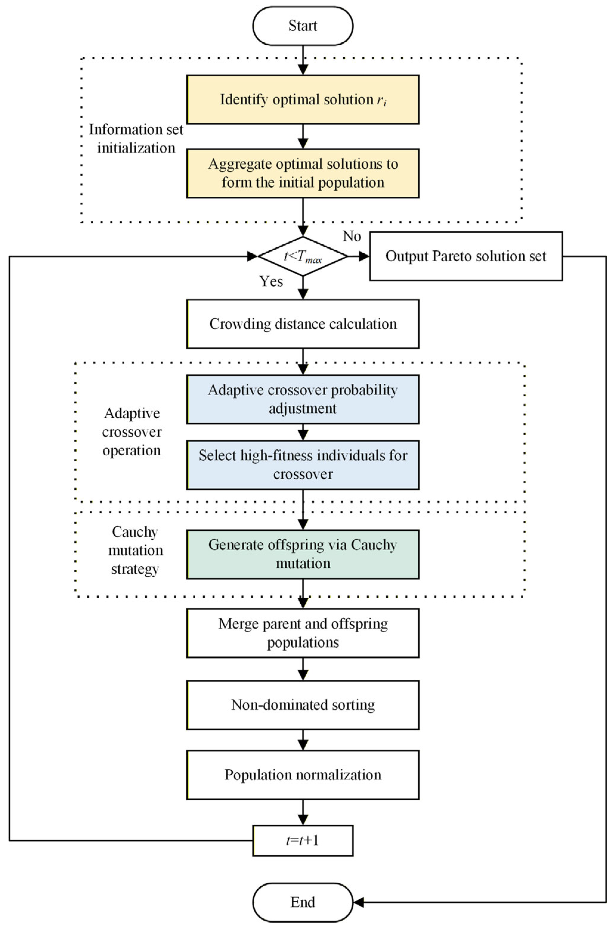
In this study, a novel GPS-AC-NSGA-III algorithm is proposed. The algorithm employs an information set initialization strategy to generate the parent population [49], utilizes an adaptive parameter adjustment strategy to regulate the dynamic crossover intensity, and incorporates a Cauchy mutation strategy during the mutation phase to expand the search space. By maintaining population diversity while enhancing convergence performance, the proposed algorithm effectively improves the global search capability.

(1)

Information set initialization strategy

The construction of the information set is based on the limiting properties of points within the set, where each point represents a unique limit point and duplication is strictly prohibited. To improve the uniformity of the initial population distribution in the decision space and enhance the early-stage exploration efficiency and global search capability of NSGA-III, an information-set-based initialization strategy is proposed. This strategy generates a set of discrete points with low discrepancy and high uniformity, thereby providing a diverse population during the initial evolutionary stage [49]. The optimal information set is constructed according to the following equations:

$$P_n(i)=\left\{(r_1{i}_1,r_2{i}_2,\cdot \cdot \cdot ,r_n{i}_n),i=1,2,\cdot \cdot \cdot ,n\right\}$$

(47)

$$r_i^k=\mathrm{mod}\left\{2i\cdot \cos ({\displaystyle \frac{2\pi k}{p}}),1\le k\le 2,1\le i\le n\right\}$$

(48)

$$P_k=\left\{(r_1^k,r_2^k,\cdot \cdot \cdot ,r_n^k),1\le k\le 2\right\}$$

(49)

where n denotes the population size, $r_i^k$ represents the optimal point, p is the smallest prime number satisfying ${\displaystyle \frac{p-3}{2}}\ge s$, and $P_k$ denotes the dimensionality of the decision space.

(2)

Adaptive crossover parameter tuning strategy

The crossover operator is a key component of NSGA-III, playing a critical role in its global search capability and overall optimization performance. To improve the algorithm’s convergence behavior, an adaptive crossover mechanism is introduced. During the early evolutionary stage, when population quality is relatively low, a higher crossover probability is employed to enhance solution space exploration and promote the discovery of promising individuals. As the evolution progresses, the crossover probability is gradually reduced to preserve high-quality genetic information from superior parent solutions and prevent excessive disruption [50]. This adaptive strategy effectively accelerates the convergence speed of NSGA-III.

$$P_{sc}=0.8+{\alpha }_c{e}^{-{\beta }_c{g}_t}+{\alpha }_0\ln (1+{\delta }_c{r}_n)$$

(50)

where ${\alpha }_c$ denotes the crossover probability control function, ${\beta }_c$, ${\alpha }_0$, and ${\delta }_c$ are positive parameters, $g_t$ represents the current population iteration number, and $r_n$ indicates the non-dominated rank of the crossover and mutation individuals at the corresponding iteration.

(3)

Cauchy mutation strategy

The mutation strategy employed in this algorithm enables the generation of wider random perturbations, thereby enlarging the search space. This mechanism effectively helps the algorithm escape local optima and enhances its global convergence capability [51].

$$x^{\ast \ast }(t)=x^{\ast }(t)+\sigma \ast C(0,1)$$

(51)

where $x^{\ast }(t)$ represents the initial population, $x^{\ast \ast }(t)$ denotes the new individuals generated through Cauchy mutation, $\sigma$ is the scaling factor for the mutation step, and $C(0,1)$ is a uniformly distributed random variable in the range [0, 1] with the following probability density function:

$$f(x^{*})=\left\{\begin{array}{ll}1/(b-a)\hfill & a<x<b\hfill \\ 0\hfill & \mathrm{else}\hfill \end{array}\right\}$$

(52)

The flow of the GPS-AC-NSGA-III algorithm is shown in Figure 4.

To validate the effectiveness of the GPS-AC-NSGA-III algorithms, a comparative analysis is conducted between the proposed GPS-AC-NSGA-III algorithm and four widely used algorithms using MATLAB R2022b: NSGA-II [52], NSGA-III [53], θ-dominance based evolutionary algorithm (θ-DEA) [54], and ANSGA-III [55]. The DTLZ family of test functions is selected to evaluate performance using the Generational Distance (GD) and Inverted Generational Distance (IGD) metrics, as these functions exhibit realistic Pareto front boundaries. The maximum population size is set to N = 400, and three scenarios with different numbers of objective functions are considered. For M = 3, the maximum number of iterations is set to T_max = 400; for M = 4, T_max = 600; and for M = 10, T_max = 1000. For each scenario, ten independent runs are performed, and the best, average, and worst results are recorded. The experimental outcomes are summarized in Appendix A.

Based on the GD and IGD metrics presented in

Table A1. Generational Distance (GD) Results Obtained by Different Algorithms.

Test Function	M	Tmax	Results	NSGA-II	NSGA-III	θ-DEA	ANSGA-III	GPS-AC-NSGA-III
DTLZ1	3	400	Best	1.8235 × 10−4	2.7326 × 10−4	3.6254 × 10−4	3.5264 × 10−4	1.4625 × 10−4
			Mean	2.4325 × 10−4	3.6254 × 10−4	4.7752 × 10−4	4.6219 × 10−4	2.0687 × 10−4
			Worst	4.3251 × 10−4	3.9365 × 10−4	6.3217 × 10−4	5.9856 × 10−4	2.9635 × 10−4
	4	600	Best	4.3624 × 10−4	4.0823 × 10−4	4.0856 × 10−4	4.0603 × 10−4	4.0409 × 10−4
			Mean	4.5651 × 10−4	4.0932 × 10−4	4.0992 × 10−4	4.1263 × 10−3	4.0762 × 10−4
			Worst	4.9346 × 10−4	4.1105 × 10−4	4.1035 × 10−4	1.6320 × 10−2	4.1013 × 10−4
	10	1000	Best	7.4325 × 100	8.3685 × 10−4	8.4325 × 10−4	3.6542 × 10−3	8.2647 × 10−4
			Mean	1.8623 × 101	4.6387 × 10−3	8.4762 × 10−4	3.9754 × 10−3	8.3953 × 10−4
			Worst	1.9962 × 101	8.6582 × 10−2	8.4987 × 10−4	4.0069 × 10−3	8.4815 × 10−4
DTLZ2	3	400	Best	4.6752 × 10−4	2.8105 × 10−4	2.7632 × 10−4	3.0762 × 10−4	2.5874 × 10−4
			Mean	5.1238 × 10−4	2.8876 × 10−4	2.7865 × 10−4	3.5201 × 10−4	2.6765 × 10−4
			Worst	5.5812 × 10−4	2.9815 × 10−4	2.8268 × 10−4	3.8756 × 10−4	2.7452 × 10−4
	4	600	Best	1.6156 × 10−3	1.1986 × 10−3	1.2014 × 10−3	1.2001 × 10−3	1.1872 × 10−3
			Mean	1.7865 × 10−3	1.2045 × 10−3	1.2049 × 10−3	1.2089 × 10−3	1.2018 × 10−3
			Worst	1.9632 × 10−3	1.2096 × 10−3	1.2078 × 10−3	1.2245 × 10−3	1.2028 × 10−3
	10	1000	Best	1.1785 × 10−1	3.7456 × 10−3	3.7391 × 10−3	5.3462 × 10−3	3.6516 × 10−3
			Mean	1.2001 × 10−1	3.7954 × 10−3	3.7554 × 10−3	7.4558 × 10−3	3.6751 × 10−3
			Worst	1.2145 × 10−1	3.8167 × 10−3	3.7867 × 10−3	8.6829 × 10−3	3.7974 × 10−3
DTLZ3	3	400	Best	2.5475 × 10−2	3.1247 × 10−1	3.4741 × 10−1	2.1475 × 10−1	6.7124 × 10−3
			Mean	2.1245 × 10−1	5.4571 × 10−1	8.1247 × 10−1	6.1376 × 10−1	4.4272 × 10−2
			Worst	6.1124 × 10−1	9.5417 × 10−1	1.0745 × 100	9.7074 × 10−1	2.0475 × 10−1
	4	600	Best	1.3842 × 10−3	1.2154 × 10−3	1.2247 × 10−3	1.2014 × 10−3	1.1902 × 10−3
			Mean	3.3067 × 10−1	1.2335 × 10−3	1.2284 × 10−3	4.5764 × 10−2	1.2126 × 10−3
			Worst	1.2874 × 100	1.2647 × 10−3	1.2453 × 10−3	4.3501 × 10−1	1.2201 × 10−3
	10	1000	Best	1.0341 × 102	3.7534 × 10−3	3.8251 × 10−3	2.5437 × 10−1	3.6897 × 10−3
			Mean	1.0413 × 102	4.8334 × 10−3	2.4376 × 10−1	1.9200 × 100	4.8241 × 10−2
			Worst	1.0468 × 102	4.9871 × 10−3	2.5014 × 100	3.6773 × 100	4.1495 × 10−1
DTLZ4	3	400	Best	4.6528 × 10−4	2.8456 × 10−4	2.6252 × 10−4	3.0429 × 10−4	2.4515 × 10−4
			Mean	4.8916 × 10−4	2.9945 × 10−4	2.7439 × 10−4	3.2542 × 10−4	2.6215 × 10−4
			Worst	5.0456 × 10−4	3.3446 × 10−4	2.8327 × 10−4	3.4129 × 10−4	2.7341 × 10−4
	4	600	Best	1.7245 × 10−3	1.1975 × 10−3	1.2038 × 10−3	1.1778 × 10−3	1.1704 × 10−3
			Mean	1.8215 × 10−3	1.2145 × 10−3	1.2166 × 10−3	1.1997 × 10−3	1.1936 × 10−3
			Worst	1.8971 × 10−3	1.2275 × 10−3	1.2232 × 10−3	1.2178 × 10−3	1.2138 × 10−3
	10	1000	Best	1.1874 × 10−1	3.7376 × 10−3	3.7211 × 10−3	3.7476 × 10−3	3.8038 × 10−3
			Mean	1.1964 × 10−1	4.2138 × 10−3	3.8476 × 10−3	4.3732 × 10−3	3.8254 × 10−3
			Worst	1.2075 × 10−1	8.0433 × 10−3	3.9694 × 10−3	4.7647 × 10−3	3.9687 × 10−3
DTLZ5	3	400	Best	3.3162 × 10−5	4.6323 × 10−5	1.5364 × 10−4	4.7653 × 10−5	2.7687 × 10−5
			Mean	4.1479 × 10−5	5.5797 × 10−5	2.7407 × 10−4	5.4378 × 10−5	4.0126 × 10−5
			Worst	4.4469 × 10−5	6.8623 × 10−5	3.0498 × 10−4	6.3765 × 10−5	6.1967 × 10−5
	4	600	Best	6.1614 × 10−2	5.9416 × 10−4	4.5461 × 10−2	2.4238 × 10−4	5.1379 × 10−3
			Mean	6.4213 × 10−2	2.4236 × 10−3	5.2501 × 10−2	1.7789 × 10−3	7.8641 × 10−3
			Worst	6.4842 × 10−2	5.6284 × 10−3	8.7443 × 10−2	3.1925 × 10−3	9.7956 × 10−3
	10	1000	Best	1.1896 × 10−1	6.4896 × 10−2	5.8631 × 10−2	6.5812 × 10−2	1.0312 × 10−1
			Mean	1.2245 × 10−1	8.3413 × 10−2	7.7627 × 10−2	8.3647 × 10−2	1.1251 × 10−1
			Worst	1.2412 × 10−1	9.5412 × 10−2	1.0365 × 10−1	1.0964 × 10−1	1.1864 × 10−1
DTLZ6	3	400	Best	2.3562 × 10−6	2.1127 × 10−6	2.1752 × 10−6	2.2245 × 10−6	2.2476 × 10−6
			Mean	2.4389 × 10−6	2.2963 × 10−6	2.3647 × 10−6	2.2869 × 10−6	2.2795 × 10−6
			Worst	2.5217 × 10−6	2.5017 × 10−6	2.6847 × 10−6	2.3483 × 10−6	2.3143 × 10−6
	4	600	Best	2.1567 × 10−1	4.9301 × 10−2	1.3761 × 10−1	9.0752 × 10−2	4.7762 × 10−2
			Mean	2.2123 × 10−1	8.6324 × 10−2	1.6213 × 10−1	9.4215 × 10−2	7.6641 × 10−2
			Worst	2.2896 × 10−1	1.1298 × 10−1	1.9467 × 10−1	1.0867 × 10−1	8.9627 × 10−2
	10	1000	Best	5.0213 × 10−1	2.7021 × 10−1	1.0492 × 10−1	3.0896 × 10−1	2.8923 × 10−1
			Mean	5.0438 × 10−1	3.3452 × 10−1	1.1476 × 10−1	3.4632 × 10−1	3.3024 × 10−1
			Worst	5.0674 × 10−1	3.5413 × 10−1	1.2341 × 10−1	3.8321 × 10−1	3.6141 × 10−1
DTLZ7	3	400	Best	9.4247 × 10−4	8.5107 × 10−4	7.0132 × 10−4	9.6296−4	5.5765 × 10−4
			Mean	1.0127 × 10−3	9.4472 × 10−4	7.3161 × 10−4	9.1210 × 10−4	6.3607 × 10−4
			Worst	1.1324 × 10−3	1.0841 × 10−3	7.8446 × 10−4	1.0287 × 10−3	7.5107 × 10−4
	4	600	Best	5.2383 × 10−3	3.1674 × 10−3	2.5157 × 10−3	3.4644 × 10−3	2.4741 × 10−3
			Mean	5.3684 × 10−3	3.5646 × 10−3	2.9641 × 10−3	3.6132 × 10−3	2.7164 × 10−3
			Worst	5.5221 × 10−3	3.8147 × 10−3	3.4527 × 10−3	4.1246 × 10−3	3.4564 × 10−3
	10	1000	Best	1.5894 × 100	4.2245 × 10−2	1.8478 × 10−2	3.7123 × 10−2	1.9262 × 10−2
			Mean	1.7242 × 100	4.3271 × 10−2	2.047 × 10−2	4.0129 × 10−2	3.4722 × 10−2
			Worst	1.8851 × 100	4.5782 × 10−2	2.4013 × 10−2	4.3484 × 10−2	5.0195 × 10−2

Note: Bold values indicate the best performance, and the same applies to the following tables.

and

Table A2. Inverted Generational Distance (IGD) Results Obtained by Different Algorithms.

Test Function	M	Tmax	Results	NSGA-II	NSGA-III	θ-DEA	ANSGA-III	GPS-AC-NSGA-III
DTLZ1	3	400	Best	1.3745 × 10−2	1.1475 × 10−2	1.1967 × 10−2	1.1458 × 10−2	1.0148 × 10−2
			Mean	1.4156 × 10−2	1.2457 × 10−2	1.3574 × 10−2	1.3716 × 10−2	1.0742 × 10−2
			Worst	1.5451 × 10−2	1.3549 × 10−2	1.4577 × 10−2	1.5642 × 10−2	1.1114 × 10−2
	4	600	Best	3.2457 × 10−2	2.6228 × 10−2	2.6224 × 10−2	2.6254 × 10−2	2.6220 × 10−2
			Mean	3.3767 × 10−2	2.6247 × 10−2	2.6247 × 10−2	2.8454 × 10−2	2.6237 × 10−2
			Worst	3.4755 × 10−2	2.6254 × 10−2	2.6258 × 10−2	3.2278 × 10−2	2.6240 × 10−2
	10	1000	Best	2.4547 × 100	1.1457 × 10−1	1.0876 × 10−1	1.1214 × 10−1	1.0871 × 10−1
			Mean	7.3234 × 100	1.5787 × 10−1	1.0884 × 10−1	1.6745 × 10−1	1.0881 × 10−1
			Worst	9.8476 × 100	1.6751 × 10−1	1.0996 × 10−1	1.8754 × 10−1	1.0896 × 10−1
DTLZ2	3	400	Best	3.2874 × 10−2	2.5672 × 10−2	2.5663 × 10−2	2.6887 × 10−2	2.5498 × 10−2
			Mean	3.4962 × 10−2	2.5717 × 10−2	2.5726 × 10−2	2.7413 × 10−2	2.5603 × 10−2
			Worst	3.6741 × 10−2	2.5758 × 10−2	2.5771 × 10−2	2.7962 × 10−2	2.5709 × 10−2
	4	600	Best	8.8512 × 10−2	7.7821 × 10−2	7.7834 × 10−2	7.8624 × 10−2	7.7804 × 10−2
			Mean	9.5243 × 10−2	7.7864 × 10−2	7.7838 × 10−2	7.8954 × 10−2	7.7824 × 10−2
			Worst	9.9123 × 10−2	7.7896 × 10−2	7.7840 × 10−2	7.9045 × 10−2	7.7829 × 10−2
	10	1000	Best	1.3698 × 100	4.2105 × 10−1	4.2067 × 10−1	4.3498 × 10−1	4.2014 × 10−1
			Mean	1.7452 × 100	4.2172 × 10−1	4.2087 × 10−1	4.9421 × 10−1	4.2076 × 10−1
			Worst	2.1236 × 100	4.2197 × 10−1	4.2103 × 10−1	6.8756 × 10−1	4.2103 × 10−1
DTLZ3	3	400	Best	0.0962 × 100	1.7364 × 100	2.7345 × 100	1.3768 × 100	1.2798 × 10−1
			Mean	1.2126 × 100	3.1567 × 100	4.5987 × 100	2.7623 × 100	3.5412 × 10−1
			Worst	3.5887 × 100	3.3687 × 100	5.9347 × 100	4.2123 × 100	1.4021 × 100
	4	600	Best	9.2142 × 10−2	7.7962 × 10−2	7.7947 × 10−2	8.2412 × 10−2	7.7742 × 10−2
			Mean	9.7604 × 10−2	7.8324 × 10−2	7.8307 × 10−2	8.7658 × 10−2	7.8045 × 10−2
			Worst	9.9842 × 10−2	7.8456 × 10−2	7.9023 × 10−2	9.1254 × 10−2	7.8497 × 10−2
	10	1000	Best	1.2796 × 103	4.2007 × 10−1	4.1906 × 10−1	4.5628 × 10−1	4.1765 × 10−1
			Mean	1.3915 × 103	4.2108 × 10−1	4.3525 × 10−1	6.7632 × 10−1	4.1879 × 10−1
			Worst	1.4218 × 103	4.2108 × 10−1	5.7632 × 10−1	8.1165 × 10−1	4.7324 × 10−1
DTLZ4	3	400	Best	3.4632 × 10−2	2.5769 × 10−2	2.5632 × 10−2	2.6358 × 10−2	2.5496 × 10−2
			Mean	3.5214 × 10−2	2.5868 × 10−2	6.5418 × 10−2	2.6908 × 10−2	2.5715 × 10−2
			Worst	3.6025 × 10−2	2.5906 × 10−2	5.8751 × 10−1	2.7168 × 10−2	2.5768 × 10−2
	4	600	Best	9.1984 × 10−2	7.7962 × 10−2	7.7875 × 10−2	7.8278 × 10−2	7.7803 × 10−2
			Mean	9.3285 × 10−2	7.8015 × 10−2	7.7831 × 10−2	7.8423 × 10−2	7.7903 × 10−2
			Worst	9.7451 × 10−2	7.8137 × 10−2	7.8125 × 10−2	7.8588 × 10−2	7.7987 × 10−2
	10	1000	Best	1.4123 × 100	4.1998 × 10−1	4.1995 × 10−1	4.2075 × 10−1	4.1982 × 10−1
			Mean	1.7862 × 100	4.3145 × 10−1	4.2005 × 10−1	4.2787 × 10−1	4.2039 × 10−1
			Worst	2.3768 × 100	4.8967 × 10−1	4.2107 × 10−1	4.8697 × 10−1	4.2046 × 10−1
DTLZ5	3	400	Best	1.4689 × 10−3	2.3126 × 10−3	1.1025 × 10−2	2.4521 × 10−3	3.3741 × 10−3
			Mean	1.5213 × 10−3	3.4587 × 10−3	1.1784 × 10−2	2.5634 × 10−3	5.0743 × 10−3
			Worst	1.5697 × 10−3	4.7854 × 10−3	1.3247 × 10−2	3.2458 × 10−3	5.2416 × 10−3
	4	600	Best	1.5478 × 10−2	9.9751 × 10−3	4.4785 × 10−2	1.3458 × 10−2	1.2784 × 10−2
			Mean	1.6785 × 10−2	1.8754 × 10−2	5.7854 × 10−2	1.9871 × 10−2	1.7621 × 10−2
			Worst	1.8742 × 10−2	4.3145 × 10−2	6.4679 × 10−2	2.7387 × 10−2	1.8235 × 10−2
	10	1000	Best	7.8954 × 10−2	2.7452 × 10−1	7.2145 × 10−2	2.7458 × 10−1	3.8741 × 10−1
			Mean	1.3784 × 10−1	3.4858 × 10−1	1.6127 × 10−1	3.5478 × 10−1	5.1425 × 10−1
			Worst	2.4852 × 10−1	4.1745 × 10−1	2.4522 × 10−1	3.9565 × 10−1	6.6785 × 10−1
DTLZ6	3	400	Best	1.3385 × 10−3	4.1425 × 10−3	1.5874 × 10−2	2.7842 × 10−3	6.7845 × 10−3
			Mean	1.4752 × 10−3	4.7458 × 10−3	1.6432 × 10−2	3.2584 × 10−3	7.4565 × 10−3
			Worst	1.5368 × 10−3	5.2459 × 10−3	1.7215 × 10−2	3.7456 × 10−3	7.7854 × 10−3
	4	600	Best	3.3795 × 10−2	1.9124 × 10−2	6.2142 × 10−2	2.4214 × 10−2	1.8468 × 10−2
			Mean	3.7541 × 10−2	4.0214 × 10−2	1.2418 × 10−1	3.6782 × 10−2	3.3587 × 10−2
			Worst	4.8962 × 10−2	1.0542 × 10−1	2.2417 × 10−1	4.9532 × 10−2	4.8247 × 10−2
	10	1000	Best	3.7896 × 100	2.7452 × 10−1	2.3451 × 10−1	4.1278 × 10−1	2.7324 × 10−1
			Mean	5.1745 × 100	4.8962 × 10−1	2.7356 × 10−1	7.4521 × 10−1	5.1425 × 10−1
			Worst	6.6874 × 100	7.1027 × 10−1	3.5432 × 10−1	1.0227 × 100	6.8561 × 10−1
DTLZ7	3	400	Best	3.6875 × 10−2	3.5127 × 10−2	3.8569 × 10−2	3.4478 × 10−2	3.3758 × 10−2
			Mean	3.7852 × 10−2	3.6238 × 10−2	4.0127 × 10−2	3.5487 × 10−2	3.4975 × 10−2
			Worst	3.8452 × 10−2	3.7648 × 10−2	4.1728 × 10−2	3.6259 × 10−2	3.5432 × 10−2
	4	600	Best	1.2084 × 10−1	1.0965 × 10−1	1.1945 × 10−1	1.0855 × 10−1	1.0398 × 10−1
			Mean	1.2243 × 10−1	1.1125 × 10−1	1.2962 × 10−1	1.1025 × 10−1	1.0754 × 10−1
			Worst	1.2745 × 10−1	1.1587 × 10−1	1.3544 × 10−1	1.1824 × 10−1	1.1420 × 10−1
	10	1000	Best	1.6125 × 100	1.0682 × 100	1.0487 × 100	9.9605 × 10−1	1.0187 × 100
			Mean	1.6568 × 100	1.1354 × 100	1.1168 × 100	1.1089 × 100	1.0762 × 100
			Worst	1.7249 × 100	1.3458 × 100	1.2152 × 100	1.3459 × 100	1.2047 × 100

in Appendix A, the proposed GPS-AC-NSGA-III algorithm demonstrates superior performance compared to the other four algorithms across most DTLZ test functions, with the best outcomes highlighted in bold.

In this section, we also conduct an ablation study on the GPS-AC-NSGA-III algorithm to validate the contribution of each component relative to the original algorithm. The variant incorporating only the improved initialization strategy is denoted as NSGA-III-GPS, the variant incorporating only the adaptive crossover strategy is denoted as NSGA-III-AC, and the variant incorporating the Cauchy mutation is denoted as NSGA-III-CM. These three algorithms are compared with NSGA-III and the full GPS-AC-NSGA-III algorithm. The resulting GD and IGD values are presented in

Table A3. GD performance of ablation variants.

Test Function	M	Tmax	Results	NSGA-III-GPS	NSGA-III-AC	NSGA-III-CM	NSGA-III	GPS-AC-NSGA-III
DTLZ1	3	400	Best	1.8238 × 10−4	1.9050 × 10−4	2.1164 × 10−4	2.7326 × 10−4	1.4625 × 10−4
			Mean	2.1305 × 10−4	2.3070 × 10−4	2.3176 × 10−4	3.6254 × 10−4	2.0687 × 10−4
			Worst	3.1057 × 10−4	2.9687 × 10−4	2.9867 × 10−4	3.9365 × 10−4	2.9635 × 10−4
	4	600	Best	4.0914 × 10−4	4.0802 × 10−4	4.0674 × 10−4	4.0823 × 10−4	4.0409 × 10−4
			Mean	6.0302 × 10−4	4.0841 × 10−4	4.0934 × 10−4	4.0932 × 10−4	4.0762 × 10−4
			Worst	8.2157 × 10−4	4.1098 × 10−4	4.1075 × 10−4	4.1105 × 10−4	4.1013 × 10−4
	10	1000	Best	8.3264 × 10−4	8.2741 × 10−4	8.2967 × 10−4	8.3685 × 10−4	8.2647 × 10−4
			Mean	9.2832 × 10−4	8.2825 × 10−4	1.0972 × 10−3	4.6387 × 10−3	8.3953 × 10−4
			Worst	9.9357 × 10−4	8.5214 × 10−4	1.4954 × 10−3	8.6582 × 10−2	8.4815 × 10−4
DTLZ2	3	400	Best	2.5961 × 10−4	2.5882 × 10−4	2.6014 × 10−4	2.8105 × 10−4	2.5874 × 10−4
			Mean	2.8498 × 10−4	2.6978 × 10−4	2.7664 × 10−4	2.8876 × 10−4	2.6765 × 10−4
			Worst	2.9776 × 10−4	2.7365 × 10−4	2.8676 × 10−4	2.9815 × 10−4	2.7452 × 10−4
	4	600	Best	1.1906 × 10−3	1.1964 × 10−3	1.1987 × 10−3	1.1986 × 10−3	1.1872 × 10−3
			Mean	1.2015 × 10−3	1.2028 × 10−3	1.2052 × 10−3	1.2045 × 10−3	1.2018 × 10−3
			Worst	1.2092 × 10−3	1.2062 × 10−3	1.2124 × 10−3	1.2096 × 10−3	1.2028 × 10−3
	10	1000	Best	3.7245 × 10−3	3.6701 × 10−3	3.7501 × 10−3	3.7456 × 10−3	3.6516 × 10−3
			Mean	3.8124 × 10−3	3.6825 × 10−3	3.7632 × 10−3	3.7954 × 10−3	3.6751 × 10−3
			Worst	3.8179 × 10−3	3.8025 × 10−3	3.7998 × 10−3	3.8167 × 10−3	3.7974 × 10−3
DTLZ3	3	400	Best	6.7521 × 10−3	9.6865 × 10−3	8.2871 × 10−3	3.1247 × 10−1	6.7124 × 10−3
			Mean	9.2459 × 10−2	5.6339 × 10−2	6.1195 × 10−2	5.4571 × 10−1	4.4272 × 10−2
			Worst	2.2147 × 10−1	3.7216 × 10−1	2.3674 × 10−1	9.5417 × 10−1	2.0475 × 10−1
	4	600	Best	1.2147 × 10−3	1.2062 × 10−3	1.3175 × 10−3	1.2154 × 10−3	1.1902 × 10−3
			Mean	1.2276 × 10−3	1.2189 × 10−3	1.3687 × 10−3	1.2335 × 10−3	1.2126 × 10−3
			Worst	1.2403 × 10−3	1.2267 × 10−3	1.3964 × 10−3	1.2647 × 10−3	1.2201 × 10−3
	10	1000	Best	6.7541 × 10−3	9.6512 × 10−3	8.13548 × 10−3	3.7534 × 10−3	3.6897 × 10−3
			Mean	8.6838 × 10−3	3.9652 × 10−2	5.7688 × 10−2	4.8334 × 10−3	4.8241 × 10−2
			Worst	1.2568 × 10−2	6.2135 × 10−1	4.8765 × 10−1	4.9871 × 10−3	4.1495 × 10−1
DTLZ4	3	400	Best	2.6741 × 10−4	2.7514 × 10−4	2.4498 × 10−4	2.8456 × 10−4	2.4515 × 10−4
			Mean	4.5866 × 10−4	4.2470 × 10−4	3.1678 × 10−4	2.9945 × 10−4	2.6215 × 10−4
			Worst	3.1364 × 10−4	2.8746 × 10−4	3.2136 × 10−4	3.3446 × 10−4	2.7341 × 10−4
	4	600	Best	1.1765 × 10−3	1.1887 × 10−3	1.1962 × 10−3	1.1975 × 10−3	1.1704 × 10−3
			Mean	1.2012 × 10−3	1.1985 × 10−3	1.2168 × 10−3	1.2145 × 10−3	1.1936 × 10−3
			Worst	1.2268 × 10−3	1.2047 × 10−3	1.2254 × 10−3	1.2275 × 10−3	1.2138 × 10−3
	10	1000	Best	3.7982 × 10−3	3.8078 × 10−3	3.8245 × 10−3	3.7376 × 10−3	3.8038 × 10−3
			Mean	3.9685 × 10−3	3.8863 × 10−3	4.1927 × 10−3	4.2138 × 10−3	3.8254 × 10−3
			Worst	3.9964 × 10−3	3.9721 × 10−3	3.9943 × 10−3	8.0433 × 10−3	3.9687 × 10−3
DTLZ5	3	400	Best	4.3132 × 10−5	4.2147 × 10−5	5.0214 × 10−5	4.6323 × 10−5	2.7687 × 10−5
			Mean	4.6861 × 10−5	4.7573 × 10−5	5.6467 × 10−5	5.5797 × 10−5	4.0126 × 10−5
			Worst	6.7423 × 10−5	6.2358 × 10−5	6.3658 × 10−5	6.8623 × 10−5	6.1967 × 10−5
	4	600	Best	5.2569 × 10−3	5.4123 × 10−3	5.3694 × 10−3	5.9416 × 10−4	5.1379 × 10−3
			Mean	6.1523 × 10−3	7.8024 × 10−3	9.9059 × 10−3	2.4236 × 10−3	7.8641 × 10−3
			Worst	9.3651 × 10−3	9.9741 × 10−3	9.9974 × 10−3	5.6284 × 10−3	9.7956 × 10−3
	10	1000	Best	1.2583 × 10−1	1.0023 × 10−1	1.2368 × 10−1	6.4896 × 10−2	1.0312 × 10−1
			Mean	1.6352 × 10−1	1.1026 × 10−1	2.3418 × 10−1	8.3413 × 10−2	1.1251 × 10−1
			Worst	1.8236 × 10−1	1.1905 × 10−1	3.4627 × 10−1	9.5412 × 10−2	1.1864 × 10−1
DTLZ6	3	400	Best	2.2698 × 10−6	2.2637 × 10−6	2.2746 × 10−6	2.1127 × 10−6	2.2476 × 10−6
			Mean	3.0104 × 10−6	2.2886 × 10−6	2.2939 × 10−6	2.2963 × 10−6	2.2795 × 10−6
			Worst	3.6014 × 10−6	2.3698 × 10−6	2.3214 × 10−6	2.5017 × 10−6	2.3143 × 10−6
	4	600	Best	4.8793 × 10−2	4.9376 × 10−2	5.0147 × 10−2	4.9301 × 10−2	4.7762 × 10−2
			Mean	7.9050 × 10−2	7.6638 × 10−2	8.3251 × 10−2	8.6324 × 10−2	7.6641 × 10−2
			Worst	9.6437 × 10−2	9.1376 × 10−2	1.0245 × 10−1	1.1298 × 10−1	8.9627 × 10−2
	10	1000	Best	2.9324 × 10−1	2.9038 × 10−1	2.9637 × 10−1	2.7021 × 10−1	2.8923 × 10−1
			Mean	3.3325 × 10−1	3.3189 × 10−1	3.3247 × 10−1	3.3452 × 10−1	3.3024 × 10−1
			Worst	3.7321 × 10−1	3.7412 × 10−1	3.5820 × 10−1	3.5413 × 10−1	3.6141 × 10−1
DTLZ7	3	400	Best	6.2145 × 10−4	5.6974 × 10−4	7.2541 × 10−4	8.5107 × 10−4	5.5765 × 10−4
			Mean	9.3380 × 10−4	7.2615 × 10−4	1.1991 × 10−3	9.4472 × 10−4	6.3607 × 10−4
			Worst	1.1235 × 10−3	9.3645 × 10−4	1.3657 × 10−3	1.0841 × 10−3	7.5107 × 10−4
	4	600	Best	2.8741 × 10−3	2.6324 × 10−3	2.5036 × 10−3	3.1674 × 10−3	2.4741 × 10−3
			Mean	3.5562 × 10−3	2.8455 × 10−3	2.8601 × 10−3	3.5646 × 10−3	2.7164 × 10−3
			Worst	3.7641 × 10−3	3.8954 × 10−3	3.5045 × 10−3	3.8147 × 10−3	3.4564 × 10−3
	10	1000	Best	3.2156 × 10−2	2.0258 × 10−2	2.7413 × 10−2	4.2245 × 10−2	1.9262 × 10−2
			Mean	4.2974 × 10−2	3.4876 × 10−2	3.6741 × 10−2	4.3271 × 10−2	3.4722 × 10−2
			Worst	5.4036 × 10−2	4.8963 × 10−2	5.1355 × 10−2	4.5782 × 10−2	5.0195 × 10−2

and

Table A4. IGD performance of ablation variants.

Test Function	M	Tmax	Results	NSGA-III-GPS	NSGA-III-AC	NSGA-III-CM	NSGA-III	GPS-AC-NSGA-III
DTLZ1	3	400	Best	1.1323 × 10−2	1.0924 × 10−2	1.0527 × 10−2	1.1475 × 10−2	1.0148 × 10−2
			Mean	1.1651 × 10−2	1.2708 × 10−2	1.1703 × 10−2	1.2457 × 10−2	1.0742 × 10−2
			Worst	1.3156 × 10−2	1.3217 × 10−2	1.3017 × 10−2	1.3549 × 10−2	1.1114 × 10−2
	4	600	Best	2.6321 × 10−2	2.6227 × 10−2	2.6212 × 10−2	2.6228 × 10−2	2.6220 × 10−2
			Mean	2.8198 × 10−2	2.6241 × 10−2	2.6218 × 10−2	2.6247 × 10−2	2.6237 × 10−2
			Worst	2.9783 × 10−2	2.6250 × 10−2	2.6241 × 10−2	2.6254 × 10−2	2.6240 × 10−2
	10	1000	Best	1.1218 × 10−1	1.0892 × 10−1	1.1296 × 10−1	1.1457 × 10−1	1.0871 × 10−1
			Mean	1.3266 × 10−1	1.0987 × 10−1	1.2574 × 10−1	1.5787 × 10−1	1.0881 × 10−1
			Worst	1.5057 × 10−1	1.0996 × 10−1	1.2671 × 10−1	1.6751 × 10−1	1.0896 × 10−1
DTLZ2	3	400	Best	2.5632 × 10−2	2.5787 × 10−2	2.5564 × 10−2	2.5672 × 10−2	2.5498 × 10−2
			Mean	3.4468 × 10−2	3.4470 × 10−2	3.4474 × 10−2	2.5717 × 10−2	2.5603 × 10−2
			Worst	4.0214 × 10−2	3.8952 × 10−2	3.6842 × 10−2	2.5758 × 10−2	2.5709 × 10−2
	4	600	Best	7.7819 × 10−2	7.7806 × 10−2	7.7826 × 10−2	7.7821 × 10−2	7.7804 × 10−2
			Mean	7.7857 × 10−2	7.7828 × 10−2	7.7902 × 10−2	7.7864 × 10−2	7.7824 × 10−2
			Worst	7.7896 × 10−2	7.7882 × 10−2	7.7936 × 10−2	7.7896 × 10−2	7.7829 × 10−2
	10	1000	Best	4.2064 × 10−1	4.2096 × 10−1	4.2103 × 10−1	4.2105 × 10−1	4.2014 × 10−1
			Mean	4.2084 × 10−1	4.2132 × 10−1	4.2235 × 10−1	4.2172 × 10−1	4.2076 × 10−1
			Worst	4.2136 × 10−1	4.2157 × 10−1	4.2269 × 10−1	4.2197 × 10−1	4.2103 × 10−1
DTLZ3	3	400	Best	2.3513 × 10−1	1.8274 × 10−1	2.9631 × 10−1	1.7364 × 100	1.2798 × 10−1
			Mean	6.2363 × 10−1	4.7367 × 10−1	7.9481 × 10−1	3.1567 × 100	3.5412 × 10−1
			Worst	1.6520 × 100	1.8214 × 100	1.7512 × 100	3.3687 × 100	1.4021 × 100
	4	600	Best	7.7953 × 10−2	7.7821 × 10−2	7.7832 × 10−2	7.7962 × 10−2	7.7742 × 10−2
			Mean	7.8279 × 10−2	7.8022 × 10−2	7.8257 × 10−2	7.8324 × 10−2	7.8045 × 10−2
			Worst	7.8521 × 10−2	7.8563 × 10−2	7.8601 × 10−2	7.8456 × 10−2	7.8497 × 10−2
	10	1000	Best	4.1982 × 10−1	4.1862 × 10−1	4.1796 × 10−1	4.2007 × 10−1	4.1765 × 10−1
			Mean	4.2212 × 10−1	4.2062 × 10−1	4.1876 × 10−1	4.2108 × 10−1	4.1879 × 10−1
			Worst	4.2425 × 10−1	4.2236 × 10−1	4.8905 × 10−1	4.2108 × 10−1	4.7324 × 10−1
DTLZ4	3	400	Best	2.5712 × 10−2	2.5568 × 10−2	2.5521 × 10−2	2.5769 × 10−2	2.5496 × 10−2
			Mean	2.5782 × 10−2	2.6271 × 10−2	5.5775 × 10−2	2.5868 × 10−2	2.5715 × 10−2
			Worst	2.5836 × 10−2	2.6621 × 10−2	2.5814 × 10−2	2.5906 × 10−2	2.5768 × 10−2
	4	600	Best	7.7921 × 10−2	7.7863 × 10−2	7.7896 × 10−2	7.7962 × 10−2	7.7803 × 10−2
			Mean	7.7982 × 10−2	7.7926 × 10−2	7.7965 × 10−2	7.8015 × 10−2	7.7903 × 10−2
			Worst	7.8065 × 10−2	7.8059 × 10−2	7.8126 × 10−2	7.8137 × 10−2	7.7987 × 10−2
	10	1000	Best	4.2015 × 10−1	4.1996 × 10−1	4.1993 × 10−1	4.1998 × 10−1	4.1982 × 10−1
			Mean	4.3123 × 10−1	4.2174 × 10−1	4.2132 × 10−1	4.3145 × 10−1	4.2039 × 10−1
			Worst	4.5201 × 10−1	4.2813 × 10−1	4.2714 × 10−1	4.8967 × 10−1	4.2046 × 10−1
DTLZ5	3	400	Best	2.2671 × 10−3	3.4561 × 10−3	4.2368 × 10−3	2.3126 × 10−3	3.3741 × 10−3
			Mean	6.4302 × 10−3	4.8809 × 10−3	5.5109 × 10−3	3.4587 × 10−3	5.0743 × 10−3
			Worst	7.1478 × 10−3	5.8432 × 10−3	6.1251 × 10−3	4.7854 × 10−3	5.2416 × 10−3
	4	600	Best	1.3954 × 10−2	1.7124 × 10−2	1.6552 × 10−2	9.9751 × 10−3	1.2784 × 10−2
			Mean	1.8862 × 10−2	1.8264 × 10−2	1.8547 × 10−2	1.8754 × 10−2	1.7621 × 10−2
			Worst	2.0156 × 10−2	1.9632 × 10−2	2.2364 × 10−2	4.3145 × 10−2	1.8235 × 10−2
	10	1000	Best	4.2587 × 10−1	2.6632 × 10−1	3.9621 × 10−1	2.7452 × 10−1	3.8741 × 10−1
			Mean	6.1235 × 10−1	4.9876 × 10−1	5.2696 × 10−1	3.4858 × 10−1	5.1425 × 10−1
			Worst	8.6512 × 10−1	6.3642 × 10−1	6.6842 × 10−1	4.1745 × 10−1	6.6785 × 10−1
DTLZ6	3	400	Best	4.3112 × 10−3	6.9542 × 10−3	8.3142 × 10−3	4.1425 × 10−3	6.7845 × 10−3
			Mean	5.0037 × 10−3	8.5431 × 10−3	1.0580 × 10−2	4.7458 × 10−3	7.4565 × 10−3
			Worst	8.1235 × 10−3	9.6328 × 10−3	1.2638 × 10−2	5.2459 × 10−3	7.7854 × 10−3
	4	600	Best	1.8930 × 10−2	1.9021 × 10−2	1.9063 × 10−2	1.9124 × 10−2	1.8468 × 10−2
			Mean	3.3611 × 10−2	3.6088 × 10−2	5.2245 × 10−2	4.0214 × 10−2	3.3587 × 10−2
			Worst	5.4136 × 10−2	5.6972 × 10−2	8.1323 × 10−2	1.0542 × 10−1	4.8247 × 10−2
	10	1000	Best	2.7462 × 10−1	2.7385 × 10−1	2.7421 × 10−1	2.7452 × 10−1	2.7324 × 10−1
			Mean	6.8952 × 10−1	4.8952 × 10−1	5.6254 × 10−1	4.8962 × 10−1	5.1425 × 10−1
			Worst	7.9025 × 10−1	6.9032 × 10−1	7.1015 × 10−1	7.1027 × 10−1	6.8561 × 10−1
DTLZ7	3	400	Best	3.4216 × 10−2	3.5057 × 10−2	3.3965 × 10−2	3.5127 × 10−2	3.3758 × 10−2
			Mean	3.5610 × 10−2	3.6137 × 10−2	3.5562 × 10−2	3.6238 × 10−2	3.4975 × 10−2
			Worst	3.6921 × 10−2	3.7521 × 10−2	3.7358 × 10−2	3.7648 × 10−2	3.5432 × 10−2
	4	600	Best	1.0689 × 10−1	1.0521 × 10−1	1.0436 × 10−1	1.0965 × 10−1	1.0398 × 10−1
			Mean	1.1128 × 10−1	1.1087 × 10−1	1.1028 × 10−1	1.1125 × 10−1	1.0754 × 10−1
			Worst	1.1532 × 10−1	1.1428 × 10−1	1.1497 × 10−1	1.1587 × 10−1	1.1420 × 10−1
	10	1000	Best	1.0598 × 100	1.0421 × 100	1.6024 × 100	1.0682 × 100	1.0187 × 100
			Mean	1.1267 × 100	1.0982 × 100	1.1336 × 100	1.1354 × 100	1.0762 × 100
			Worst	1.3103 × 100	1.2365 × 100	1.2965 × 100	1.3458 × 100	1.2047 × 100

in Appendix A. As shown in the table, the majority of the GD and IGD metrics for these three algorithms outperform those of the NSGA-III algorithm, with the GPS-AC-NSGA-III algorithm achieving the best performance. It can be concluded that each individual improvement contributes to enhancing the algorithm’s performance, and the combination of all strategies achieves the best overall performance.

4.3. CRITIC-Based TOPSIS Method

The TOPSIS method evaluates each alternative by computing its distance from both the positive and negative ideal solutions, subsequently determining the relative closeness to the ideal solution. Based on this closeness measure, the alternatives are ranked according to their overall performance. In this study, an enhanced TOPSIS method is employed, incorporating the CRITIC [56] objective weighting approach to obtain more accurate and reliable weighting factors. This facilitates the identification of the optimal operational scheme for the IES from the Pareto solution.

The CRITIC-based TOPSIS method enhances the construction of the decision matrix. A weighted standard evaluation matrix is first constructed by multiplying the evaluation matrix with the weights ω derived from the CRITIC method. Subsequently, the normalized decision matrix is multiplied by these weights to obtain the weighted normalized decision matrix. The specific steps are as follows:

(1)

Construct the evaluation matrix:

$$T=\left[\begin{array}{cccc}{c}_{11}& c_{12}& \dots & c_{1m}\\ c_{21}& c_{22}& \dots & c_{2m}\\ ⋮& ⋮& \ddots & ⋮\\ c_{n1}& c_{n2}& \dots & c_{nm}\end{array}\right]$$

(53)

where m represents the number of evaluation indicators, and n represents the number of evaluation solutions. Specifically, in this study, m corresponds to the number of objective functions, and n corresponds to the number of Pareto solutions.

(2)

Determination of Indicator Weights

The CRITIC method [56] assesses the quality of indicators from two perspectives. On one hand, it considers the standard deviation of each indicator across evaluation schemes, where a larger standard deviation indicates greater variation in the indicator values among the schemes. On the other hand, it captures the conflict among indicators by measuring their interrelationships, thereby reflecting the degree of dissimilarity between them. The specific steps are as follows: first, constructing the original evaluation matrix; second, normalizing the matrix; and finally, determining the weights $\omega$.

(3)

Construction of the Weighted Decision Matrix

$$A={(\overline{\omega } c_{ij})}_{n\times m}$$

(54)

(4)

Identification of the Positive and Negative Ideal Solutions of the Weighted Decision Matrix

$$\left\{\begin{array}{l}{V}^{+}=[(\max c_{ij};j\in J^{\prime }),(\min c_{ij};j\in J^{″}),i=1,2,\dots ,n]\\ V^{-}=[(\min c_{ij};j\in J^{\prime }),(\max c_{ij};j\in J^{″}),i=1,2,\dots ,n]\end{array}\right.$$

(55)

where $V^{+}$ denotes the positive ideal solution, $V^{-}$ denotes the negative ideal solution, and $J^{\prime }$ and $J^{″}$ represent the positive and negative indicators, respectively.

(5)

Calculate the separation distance of each solution from the positive and negative ideal solutions:

$$\left\{\begin{array}{l}PIS{d}_i^{+}=\sqrt{{\displaystyle \sum _{j=1}^m{\left(V^{+}-\left(\overline{\omega }{c}_{ij}\right)\right)}^2}}\hfill \\ NIS{d}_i^{-}=\sqrt{{\displaystyle \sum _{j=1}^m{\left(V^{-}-\left(\overline{\omega }{c}_{ij}\right)\right)}^2}}\hfill \end{array}\right.$$

(56)

where $PIS{d}_i^{+}$ and $NIS{d}_i^{-}$ denote the distances from the ith solution to the positive and negative ideal solutions, respectively.

(6)

Calculate the relative closeness coefficient for each alternative scenario:

$$C{C}_i=NIS{d}_i^{-}/(PIS{d}_i^{+}+NIS{d}_i^{-})$$

(57)

where the relative closeness coefficient is denoted as $C{C}_i\in [0,1]$, and all alternatives are subsequently ranked in descending order based on their corresponding $C{C}_i$ values.

5. Data Collection

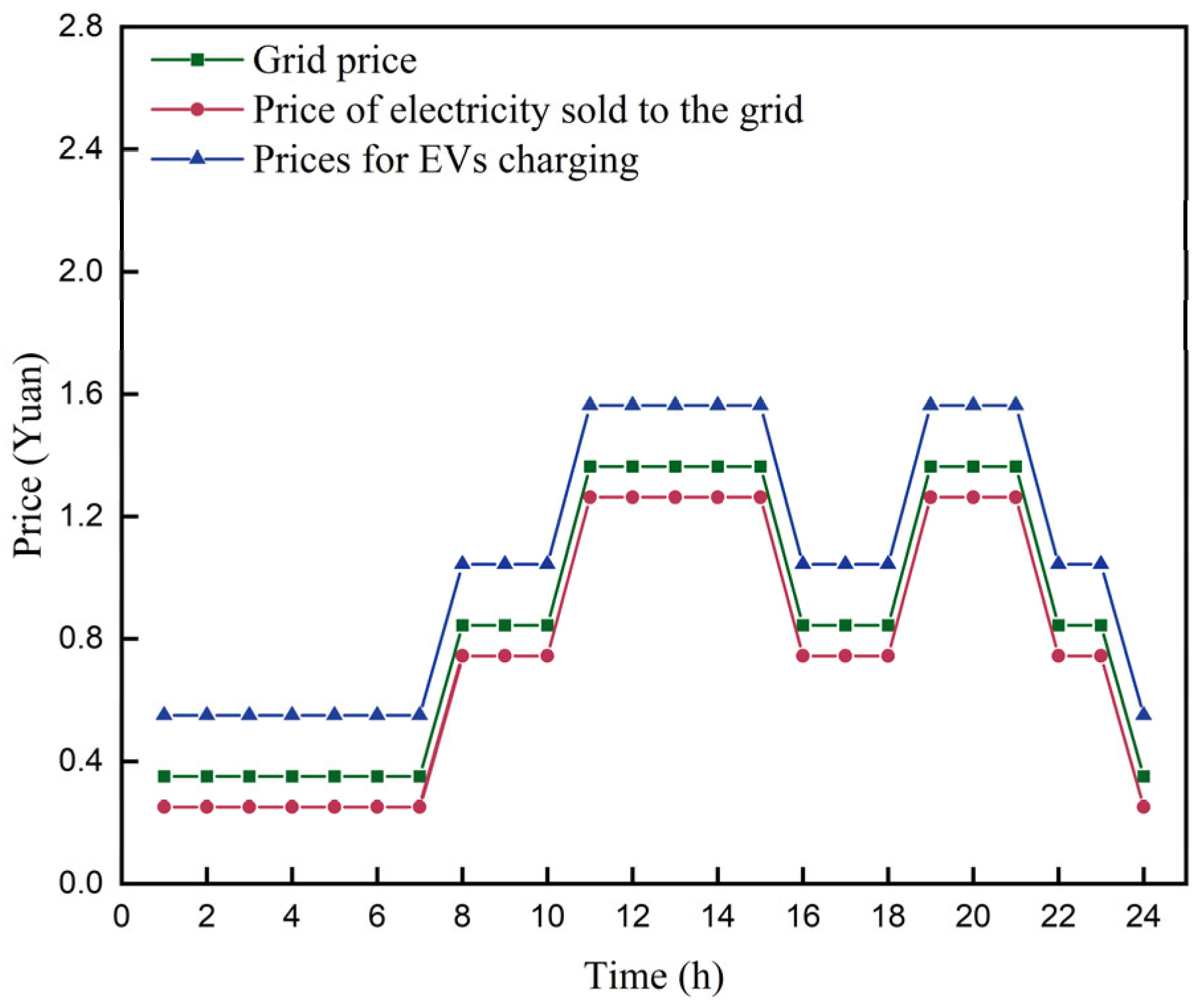
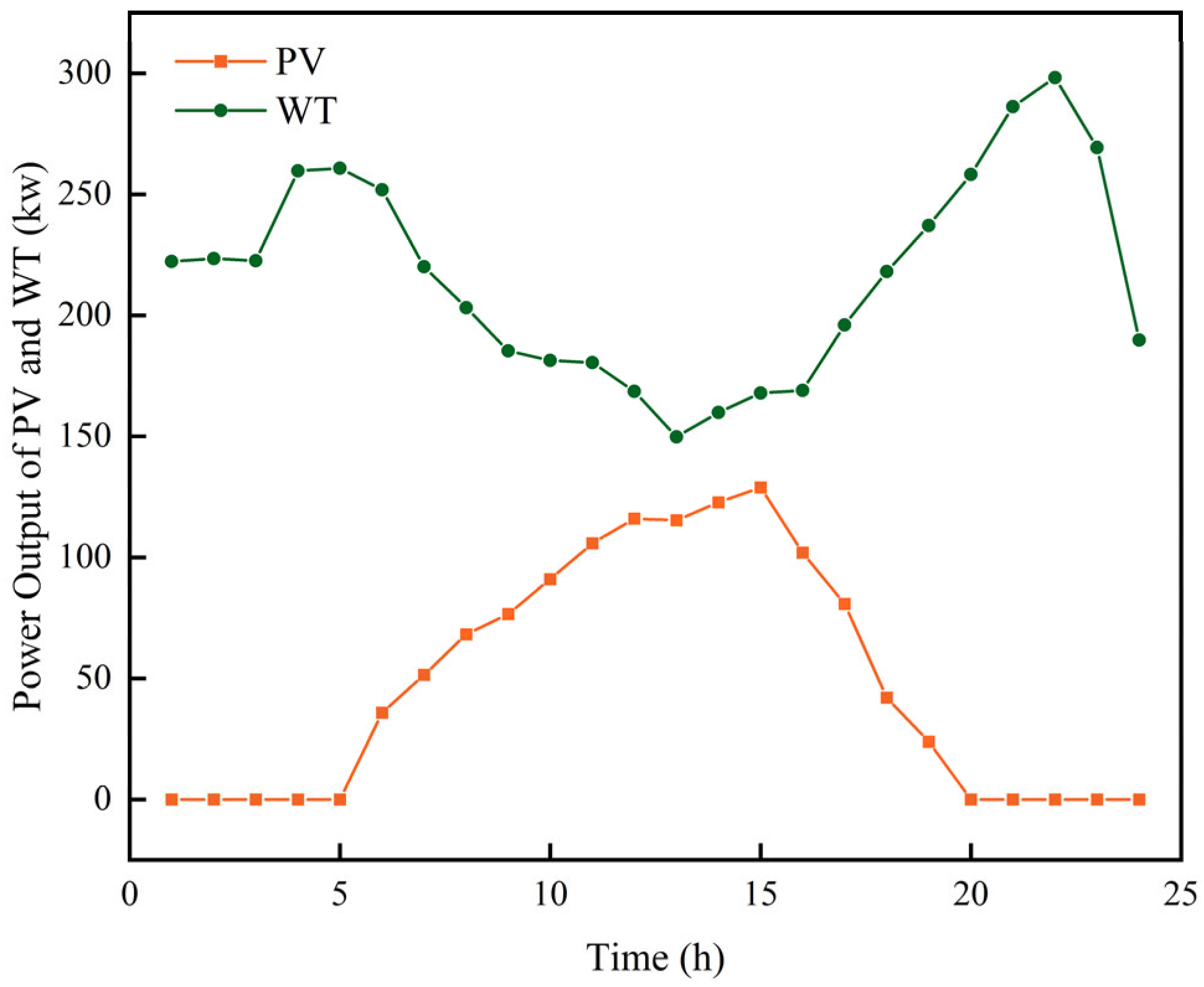
By collecting time-of-use electricity prices in Wuhan, the electricity purchasing price from the grid, the electricity selling price from the IES to the grid, and the EV charging price during each time period are summarized, as shown in Figure 5 [57]. According to the PV and wind turbine (WT) models described in Section 2.3 the power output of the PV and WT systems in the IES is calculated and presented in Figure 6 [58]. The station is equipped with 10 charging piles. The waiting time for battery exchange and hydrogen refueling is not considered. Each hydrogen vehicle has a hydrogen storage capacity of 6 kg, and the hydrogen selling price at the station is 58 RMB/kg.

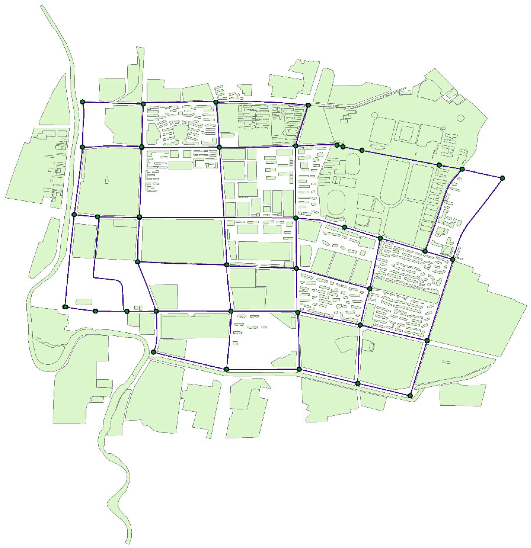
In this study, the Hongshan District of Wuhan was selected as the research area. The OpenStreetMap platform was used to extract the region with longitude and latitude ranges of [114.30412, 114.33534] × [30.49348, 30.51503]. The road network topology was then extracted using software tools such as QGIS and ArcMap. The selected area has a perimeter of approximately 11.3 km and a surface area of about 5.6 km². The geographical map of the selected area is shown in Figure 7.

6. Results and Discussions

In this study, a cooperative optimization model for NEV–IES is first constructed, followed by the proposal of the GPS-AC-NSGA-III algorithm. To verify the superior performance of the GPS-AC-NSGA-III algorithm in solving the proposed model, it is compared with four benchmark algorithms through extensive simulations. To further validate the effectiveness of the model, four case studies under different operating conditions are designed, and the GPS-AC-NSGA-III algorithm is adopted to solve and analyze each case.

6.1. Algorithm Performance Testing

In this study, the θ-DEA, NSGA-II, NSGA-III, ANSGA-III, and GPS-AC-NSGA-III algorithms are employed to simultaneously solve the collaborative optimization scheduling model for new energy vehicles and integrated energy stations. θ-DEA is a decomposition-based evolutionary algorithm that combines reference vector guidance with dominance-based selection, providing a balance between convergence and diversity. NSGA-II is a classical Pareto-based multi-objective optimization algorithm that employs non-dominated sorting and crowding distance to maintain solution diversity. NSGA-III extends NSGA-II by introducing reference points, making it more suitable for many-objective optimization problems. By integrating an adaptive mechanism into NSGA-III, ANSGA-III demonstrates superior flexibility and solution efficiency in handling complex multi-objective optimization tasks. These algorithms are selected to provide a comprehensive and structured comparison. Specifically, NSGA-II, NSGA-III, and θ-DEA represent three major categories of multi-objective optimization methods: Pareto-based, reference-point-based, and decomposition-based approaches. In addition, ANSGA-III is included to enable a fair comparison within the same algorithmic family, allowing the effectiveness of the proposed improvements over NSGA-III to be clearly demonstrated.

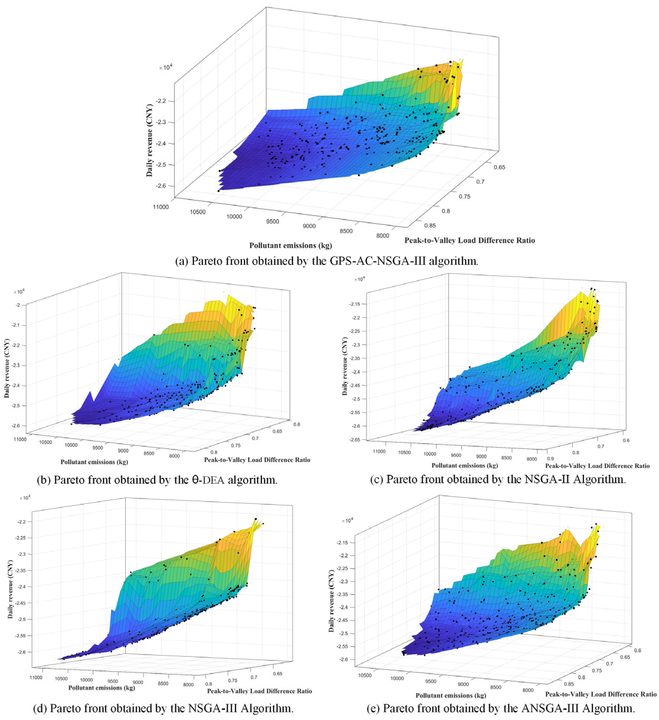
The initial population size is set to 400, and each algorithm is executed 10 times to ensure result reliability. Figure 8 illustrates the Pareto fronts obtained by the GPS-AC-NSGA-III algorithm in comparison with the other four algorithms.

The optimal solutions obtained from the solution sets of the five algorithms for the integrated energy station model were identified using the CRITIC-based TOPSIS method, as presented in

Table 3. Comparison of optimal solutions for the IES model using different algorithms.

Algorithm	Daily Revenue (CNY)	Pollutant Emissions (kg)	Peak-to-Valley Load Difference Ratio
θ-DEA	25,822.74	10,500.50	72%
NSGA-II	25,925.92	10,183.65	76%
NSGA-III	26,028.80	10,596.11	73%
ANSGA-III	25,912.82	10,591.32	73%
GPS-AC-NSGA-III	26,068.43	10,269.55	71%

Note: Bold values indicate the best performance.

(with the best results highlighted in bold). For clarity, the peak-to-valley ratio is reported in percentage form in Section 6. The optimal solution derived by the GPS-AC-NSGA-III algorithm outperforms the other four algorithms in terms of daily revenue and consistently achieves a lower Peak-to-Valley Load Difference Ratio. However, its performance with respect to pollutant emissions is relatively moderate. These findings indicate that the proposed GPS-AC-NSGA-III algorithm demonstrates strong overall effectiveness in solving the integrated energy station optimization model. Nevertheless, under scenarios with highly complex constraints, further improvements are required to enhance the algorithm’s search capability and coordination performance.

To further validate the effectiveness of the proposed algorithmic model, the Spread metric is selected to evaluate the algorithm’s performance. The Spread metric assesses the uniformity of the Pareto solution set distribution, with lower values indicating superior distribution performance, as defined in Equation (58). $d_f$ and $d_l$ represent the Euclidean distances between the extreme solutions and the boundary solutions within the set of nondominated solutions. $d_j$ denotes the Euclidean distance between the continuous solutions of the obtained set of non-dominated solutions, and $\overline{d}$ represents the average value of all values of $d_j$.

$$\Delta =(d_f+d_l+{\displaystyle \sum _{j=1}^{N-1}\left|d_j-\overline{d}\right|})/[d_f+d_l+(N-1)\overline{d}]$$

(58)

As shown in

Table 4. Algorithm Parameter Configuration.

Parameter	Symbol	Value
Population size	N	400
Maximum number of function evaluations	maxFE	40,000
Objective function	M	3
Maximum number of iterations	T	100

, to compare the performance of the algorithms in solving the proposed model, the initial population size was uniformly set to 400, the maximum number of iterations to 100, and the maximum number of function evaluations to 40,000. As shown in

Table 5. Comparison of the metric spread.

Algorithm	Best	Mean	Worst
NSGA-II	7.783 × 10−1	8.0244 × 10−1	8.364 × 10−1
NSGA-III	7.804 × 10−1	8.1943 × 10−1	8.335 × 10−1
θ-DEA	7.892 × 10−1	8.2163 × 10−1	8.566 × 10−1
ANSGA-III	7.820 × 10−1	8.2037 × 10−1	8.374 × 10−1
NSGA-III-GPS	7.8202 × 10−1	8.0084 × 10−1	8.3051 × 10−1
NSGA-III-AC	7.7927 × 10−1	7.9862 × 10−1	8.2609 × 10−1
NSGA-III-CM	7.8265 × 10−1	8.1759 × 10−1	8.2814 × 10−1
GPS-AC-NSGA-III	7.8260 × 10−1	7.9428 × 10−1	8.2310 × 10−1

Note: Bold values indicate the best performance.

, the GPS-AC-NSGA-III algorithm achieves lower mean and maximum Spread values across multiple independent runs compared to the other algorithms. (Bold indicates better results, and the same applies to the following tables.) Since a smaller Spread indicates a more uniformly distributed solution set, this result suggests that the proposed algorithm yields better solution set diversity. In terms of Processing Time presented in

Table 6. Comparison of Processing Time.

Algorithm	Best	Mean	Worst
NSGA-II	7.3365 × 100	7.8786 × 100	8.5176 × 100
NSGA-III	9.2541 × 100	1.0611 × 101	1.1127 × 101
θ-DEA	8.9624 × 100	9.2305 × 100	9.6218 × 100
ANSGA-III	9.2025 × 100	9.9479 × 100	1.4315 × 101
NSGA-III-GPS	7.1058 × 100	7.7988 × 100	8.3749 × 100
NSGA-III-AC	7.1364 × 100	8.0539 × 100	8.7623 × 100
NSGA-III-CM	7.4631 × 100	8.3415 × 100	8.9412 × 100
GPS-AC-NSGA-III	6.5137 × 100	7.2782 × 100	7.8641 × 100

, the Processing Time of the GPS-AC-NSGA-III algorithm is lower than that of the other algorithms, indicating higher computational efficiency under the same computational budget. Finally, as can be observed from the HV results in

Table 7. Comparison of Hypervolume (HV) values.

Algorithm	Best	Mean	Worst
NSGA-II	2.4018 × 10−1	1.3942 × 10−1	8.3903 × 10−2
NSGA-III	2.1526 × 10−1	1.2581 × 10−1	9.7417 × 10−2
θ-DEA	1.9235 × 10−1	1.2182 × 10−1	8.0147 × 10−2
ANSGA-III	2.3285 × 10−1	1.4227 × 10−1	1.2196 × 10−1
NSGA-III-GPS	2.4408 × 10−1	1.6371 × 10−1	1.1325 × 10−1
NSGA-III-AC	2.2517 × 10−1	1.4463 × 10−1	1.0419 × 10−1
NSGA-III-CM	2.3710 × 10−1	1.3625 × 10−1	9.8573 × 10−2
GPS-AC-NSGA-III	2.8437 × 10−1	1.8376 × 10−1	1.3315 × 10−1

, the GPS-AC-NSGA-III algorithm attains the highest hypervolume value, indicating that its solution set covers a larger region in the objective space. This further demonstrates that the algorithm is capable of obtaining a constrained Pareto front with better convergence and more uniform distribution.

6.2. Case Study

The operation of the IES model is simulated under four different conditions to empirically validate its effectiveness. The configuration of the four cases is presented in

Table 8. Strategies adopted in each case.

Case	Static Dijkstra-Based Routing	Dynamic Dijkstra-Based Routing	Time-of-Use Pricing	Dynamic Pricing Regulation
Case 1	√	×	√	×
Case 2	×	√	√	×
Case 3	√	×	×	√
Case 4	×	√	×	√

, (√ indicates that the strategy is adopted, and × indicates that it is not.) distinguishing between the static and dynamic Dijkstra algorithms as the vehicle routing strategy, and between time-of-use pricing and dynamic pricing as the energy management strategy.

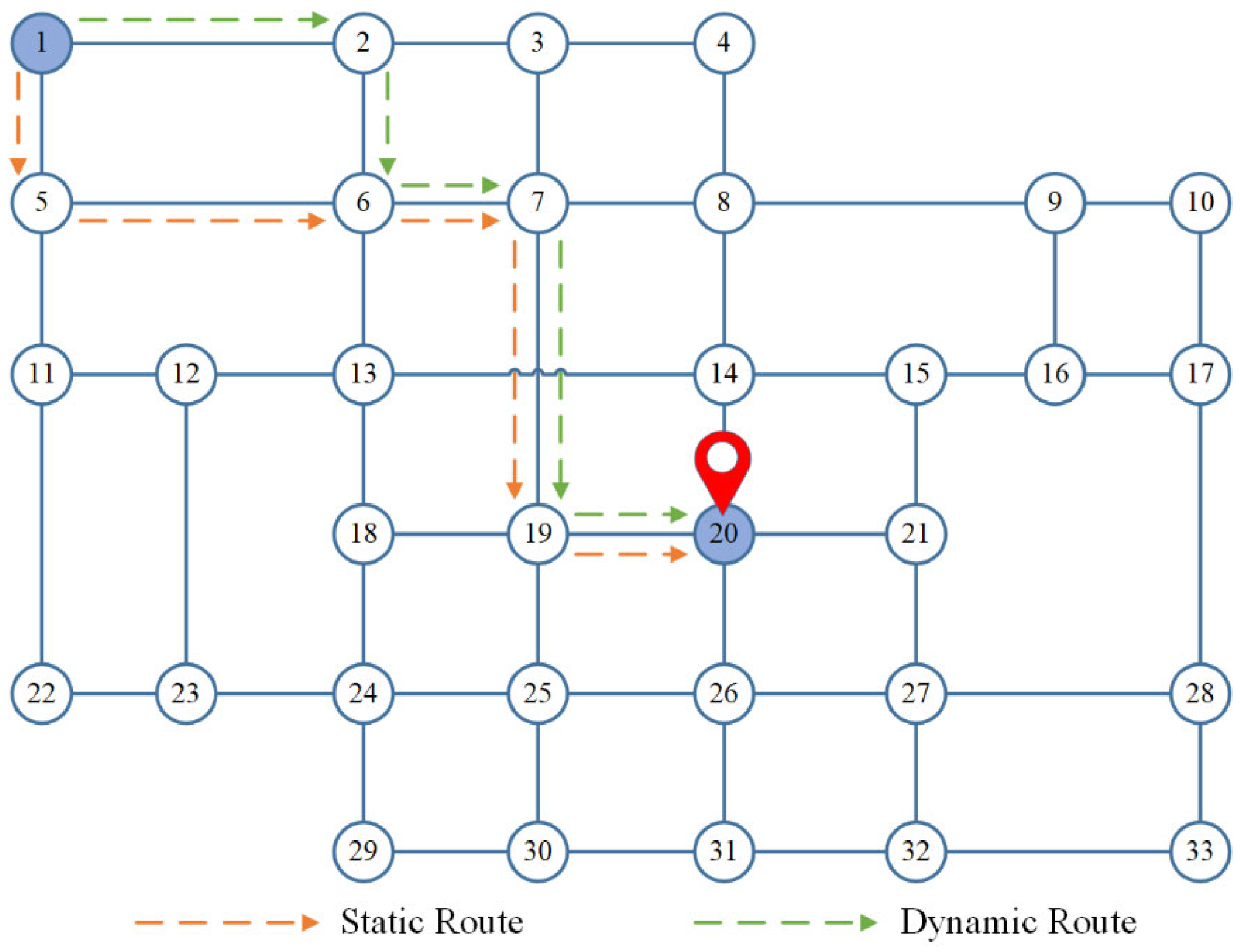
For the car’s behavior from node 1 to node 20, the two paths searched are computed using the static Dijkstra algorithm and the dynamic Dijkstra algorithm respectively as shown in Figure 9.

Table 9. Comparison of two path search methods.

Routing Strategy	Specific Route or Selected Route	Number of Traversed Nodes (Units)	Travel Distance (km)	Travel Time (s)
Static Route	1→5→6→7→19→20	6	2.90	108.21
Dynamic Route	1→2→6→7→19→20	6	3.05	99.77

presents the comparative results of the two pathfinding strategies. According to the results, there are two possible paths from Node 1 to Node 6: one via Node 2 and the other via Node 5. Based on the road resistance model, values $w_{12}=22.89$, $w_{26}=13.88$, $w_{15}=20.99$, $w_{56}=24.22$, and $w_{12}+w_{26}<w_{15}+w_{56}$ are obtained. Therefore, the dynamic algorithm selects the path 1→2→6 for vehicle routing. This pathfinding process is iteratively executed until the destination is reached, resulting in a total travel time of 108.21 s. Although the dynamic path is 0.15 km longer than the static one in terms of distance, it significantly reduces travel time compared to the static path generated by Dijkstra’s algorithm, thereby improving vehicle routing efficiency to the IES.

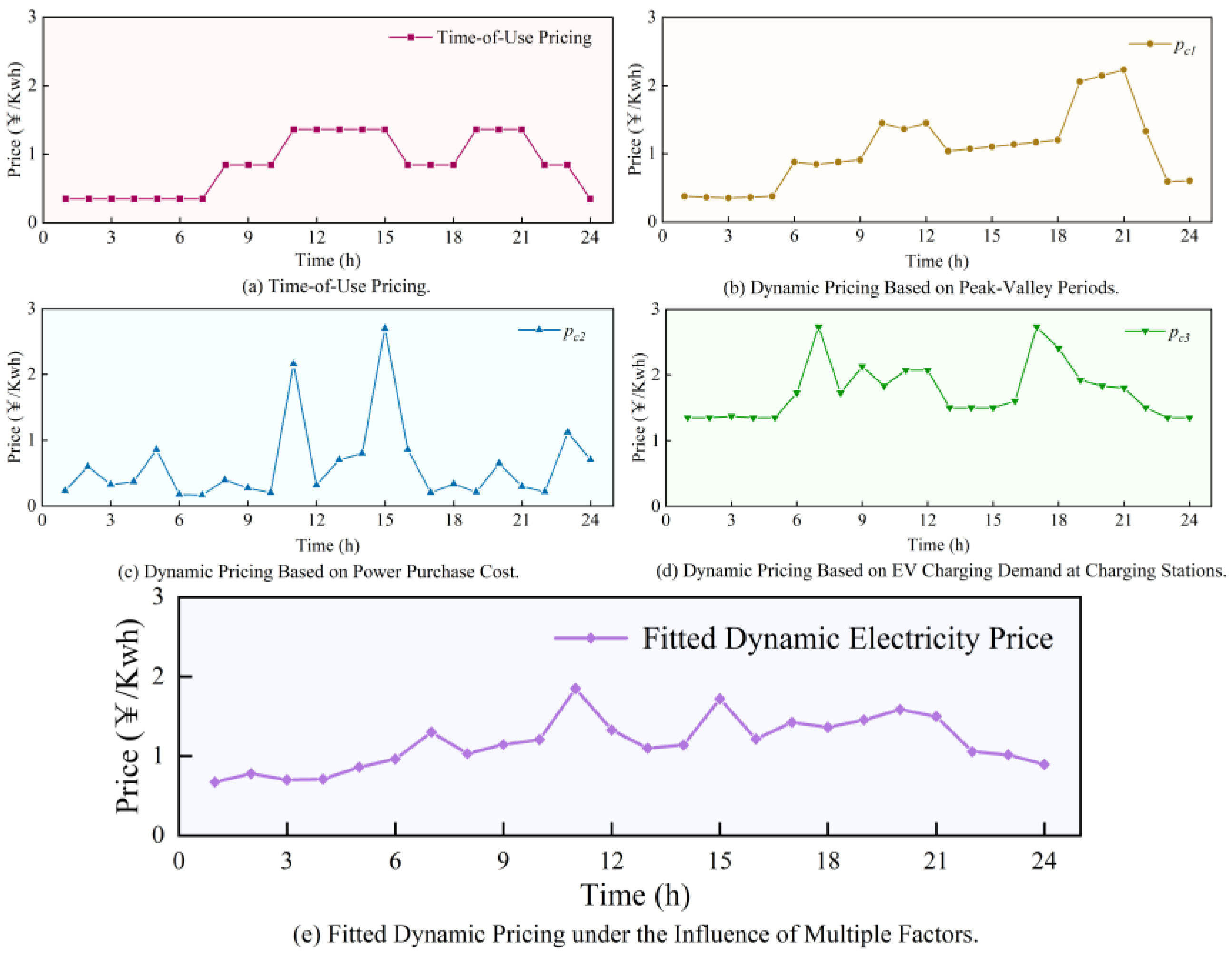
Taking into account factors such as the peak-to-valley leveling period of grid electricity prices, the power purchase cost of the IES, and the charging demand of EVs, a multi-scenario real-time dynamic pricing model is constructed using numerical methods, including the least squares method, as illustrated in Figure 10. In accordance with the previously established dynamic pricing models, the red curve represents the grid-side time-of-use tariff; the yellow curve $p_{c1}$ illustrates the dynamic pricing model based on the peak-to-valley leveling period; the blue curve $p_{c2}$ represents the dynamic pricing model influenced by grid power purchase costs; and the green curve $p_{c3}$ corresponds to the dynamic pricing model that accounts for the EV charging demand at the station. The final purple curve represents the dynamic electricity price obtained by weighted fitting of $p_{c1}$, $p_{c2}$, and $p_{c3}$ using the CRITIC method.

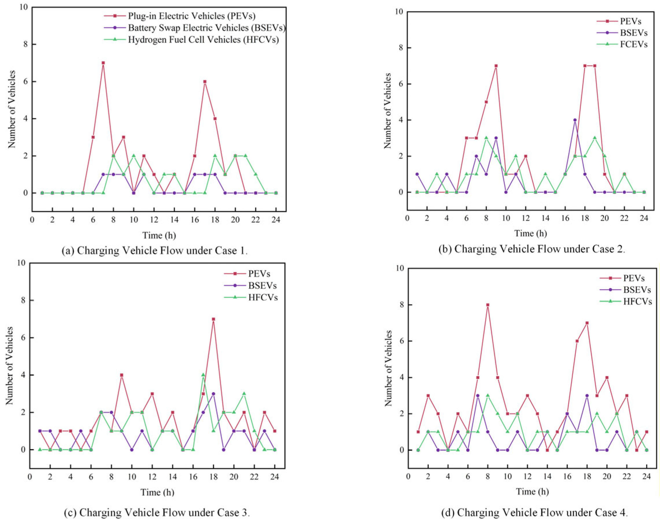
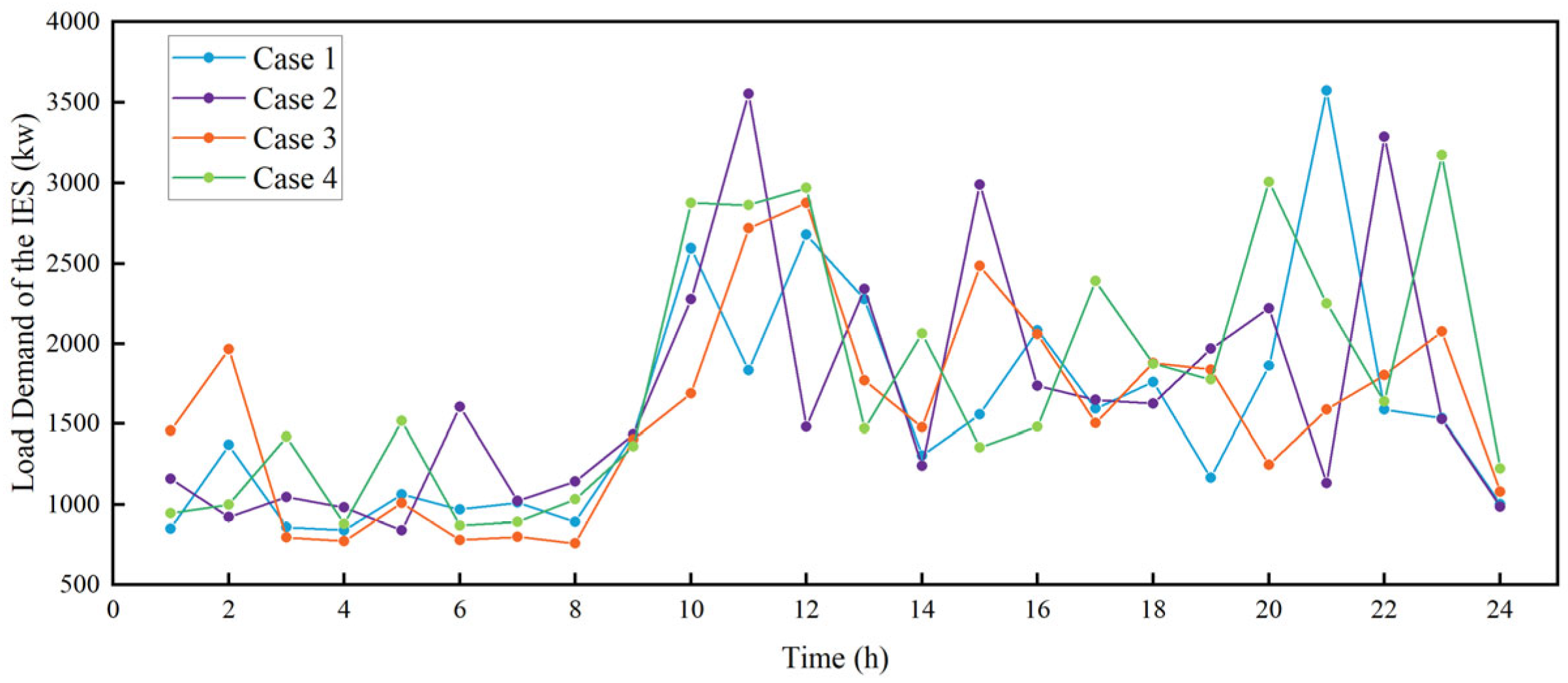
To ensure the reliability of the results, ten independent Monte Carlo simulations were conducted and the results were averaged. To facilitate the subsequent calculation of the optimization objectives for the integrated energy station using traffic flow data, the simulated traffic flow values were rounded to integers. The resulting 24 h inbound traffic flow at the station is presented in Figure 11.

Similarly, the GPS-AC-NSGA-III algorithm was employed to solve the four cases independently ten times each to obtain the optimal solutions. The mean values and standard deviations of the three objective functions for the optimal solutions in each case were calculated and are presented in

Table 10. Optimal solutions of the four cases.

Case	Daily Revenue (CNY)	Pollutant Emissions (kg)	Peak-to-Valley Load Difference Ratio
Case 1	−18,624.85 ± 258.73	10,290.29 ± 74.91	74.9% ± 1.8%
Case 2	−22,986.57 ± 267.28	10,348.27 ± 82.17	75.6% ± 2.1%
Case 3	−24,312.61 ± 293.42	10,534.75 ± 68.26	72.6% ± 1.7%
Case 4	−26,042.36 ± 262.57	10,248.76 ± 78.27	71.2% ± 1.8%

Note: Bold values indicate the best performance.

. In the following, the mean values of the optimal solutions for the three objective functions across the cases are discussed. For clarity, the peak-to-valley ratio is reported in percentage form in Section 6.

(1)

Case 1

In Case 1, vehicle owners navigate using the static Dijkstra algorithm and select the shortest route to the charging station without accounting for road congestion, which increases travel time. The charging station applies a fixed time-of-use pricing strategy based on grid electricity tariffs. Under this pricing mechanism, the tariff remains constant within each defined period. Using Monte Carlo simulation, the vehicle arrival patterns at the IES are obtained, as illustrated in Figure 11a. The results indicate that charging vehicles are highly concentrated during two peak periods: 6:00–9:00 in the morning and 17:00–20:00 in the evening. During other time slots, particularly in the early morning hours, the number of incoming vehicles is minimal. The excessive concentration of vehicles within short time windows leads to a significant increase in queuing time. Under queuing time constraints, some vehicles abandon charging, which considerably reduces the revenue of the IES. Furthermore, the uneven temporal distribution of vehicle charging causes a pronounced peak-to-valley difference in grid-side load. The optimal operational performance of Case 1, as determined using CRITIC-based TOPSIS method, yields the following results: F1 = CNY 18,624.85, F2 = 10,290.29 kg, and F3 = 74.9%.

(2)

Case 2

In Case 2, vehicle owners navigate using the dynamic Dijkstra algorithm. At each node, the vehicle compares real-time traffic conditions across connected road segments, estimates the required travel time, and selects the segment with the shortest travel time as the next path, thereby effectively avoiding congested routes. The time-varying inbound traffic flow at the IES under this case is illustrated in Figure 11b. Compared with Case 1, the dynamic routing strategy improves the efficiency of vehicle arrival, which subsequently increases the number of charging vehicles and enhances the daily revenue of the station. Under the operational conditions of Case 2, the objective values obtained are as follows: F1 = CNY 22,986.57, F2 = 10,348.27 kg, and F3 = 75.6%.

(3)

Case 3

In Case 3, the vehicle owner navigates using the static Dijkstra algorithm, while the IES adopts a dynamic tariff strategy. This strategy sets the tariff based on three factors: the peak-to-valley leveling period, the electricity procurement cost at the charging station, and the EV charging demand. Under the regulation of the dynamic pricing scheme, some EV owners opt to charge during low-tariff periods, as illustrated in Figure 11c. This behavior contributes to balancing electricity demand across different time intervals and reduces the load peak-to-valley difference at the station. Compared with Case 1, the revenue under Case 3 conditions increases slightly, while the peak-to-valley load difference is notably reduced. The optimal objective values for Case 3 are F1 = CNY 24,312.61, F2 = 10,534.75 kg, and F3 = 72.6%.

(4)

Case 4

In Case 4, vehicle owners navigate using the dynamic Dijkstra algorithm, and the IES sets tariffs based on a dynamic pricing strategy. Figure 11d illustrates the inbound traffic flow under Case 4 conditions. This case integrates the advantages of Cases 2 and 3: the dynamic Dijkstra algorithm reduces travel time and improves vehicle arrival efficiency, thereby increasing the number of charging vehicles and enhancing station revenue. Simultaneously, under the regulation of dynamic tariffs, some EV owners choose to charge during low-tariff periods. As a result, the number of vehicles entering the station for charging and battery swapping rises during these times, and the charging load becomes more evenly distributed across all time intervals. This leads to a notable reduction in the peak-to-valley load difference on the grid side. The orderly charging strategy employed in Case 4 improves vehicle charging efficiency and facilitates peak shaving and valley filling in the distribution network of the IES. The optimal objective values for Case 4 are F1 = CNY 26,042.36, F2 = 10,248.76 kg, and F3 = 71.2%.

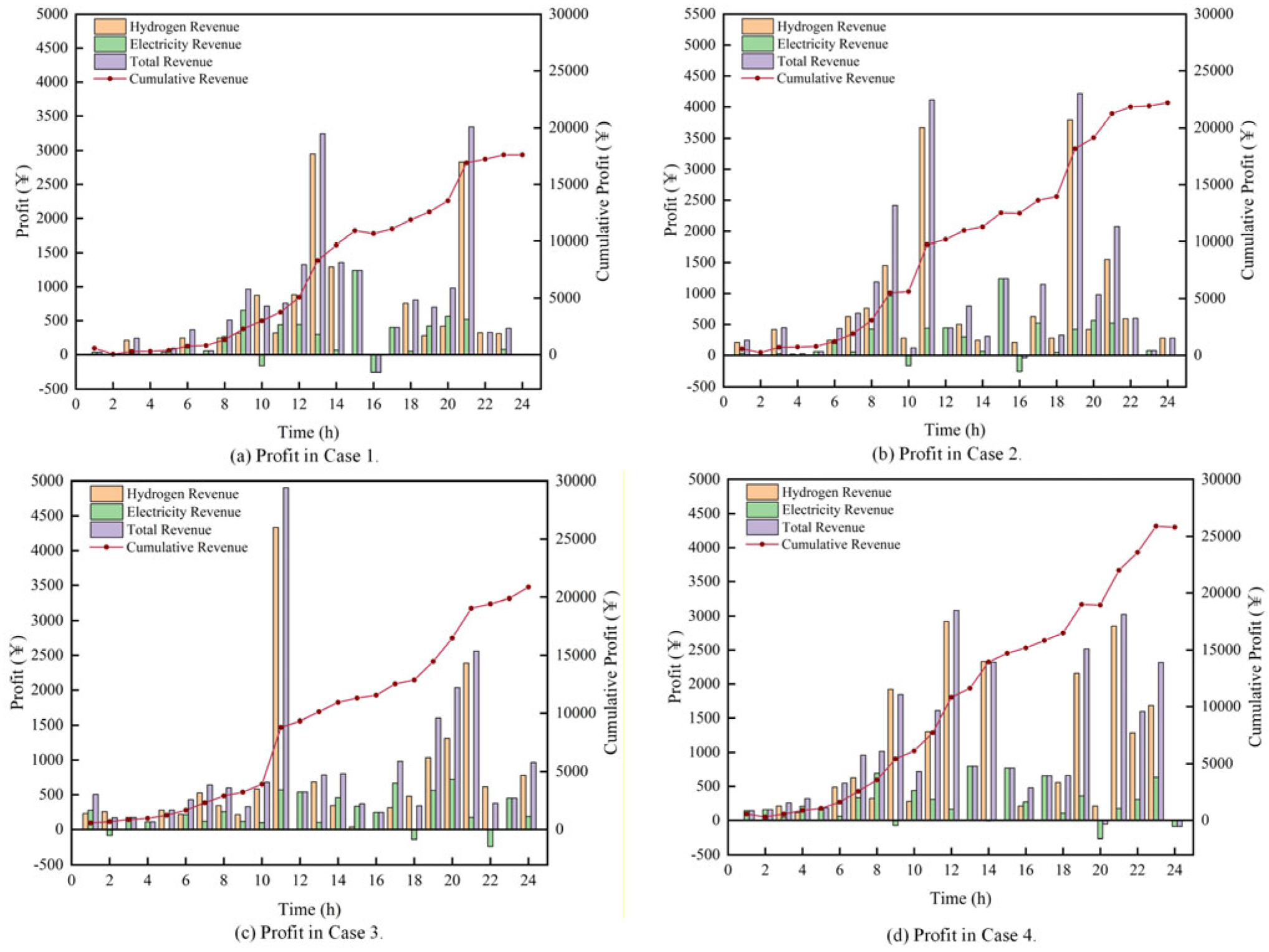
Figure 12 illustrates the daily revenues of the hydrogen energy system and the energy storage system at the IES, while Figure 13 depicts the corresponding load profiles. A comparative analysis between Case 4 and the other three cases indicates that, relative to the optimal objective outcomes in Case 3, Case 4 achieves a 7.11% increase in daily revenue, a 2.71% reduction in pollutant emissions, and a 1.93% decrease in the Peak-to-Valley Load Difference Ratio. These results demonstrate that the dynamic routing algorithm effectively improves vehicle travel efficiency and reduces unnecessary driving time, thereby indirectly enhancing charging station utilization and revenue generation.

Further comparison between Case 4 and Case 2 reveals that, under the implementation of the dynamic pricing strategy, Case 4 exhibits a 13.29% improvement in daily revenue, a 0.96% decrease in pollutant emissions, and a 5.82% reduction in the Peak-to-Valley Load Difference Ratio. This indicates that the real-time pricing mechanism not only enhances the economic performance of integrated energy stations but also more effectively guides users toward off-peak charging, thereby mitigating load fluctuations within the stations.

Finally, Case 4 demonstrates a more pronounced performance improvement compared with Case 1, with daily revenue increasing by 39.83%, pollutant emissions decreasing by 0.40%, and the Peak-to-Valley Load Difference Ratio declining by 4.94%. Since pollutant emissions are associated with the electricity purchased by the integrated energy station, the volume of charging traffic in Case 1 is relatively low compared to that in Case 4. As a result, the reduction in pollutant emissions is not sufficiently pronounced. Moreover, the mean results remain consistent across repeated experiments, suggesting that this observation is not attributable to stochastic variations. Consequently, the proposed collaborative optimization model for new energy vehicles and integrated energy stations, which integrates the dynamic Dijkstra-based routing strategy with the dynamic pricing regulation mechanism, exhibits superior performance in terms of economic efficiency, emission reduction, and load fluctuation suppression, contributing to enhanced operational stability and safety of the power grid.

A sensitivity analysis is conducted on the weighting coefficients for selecting the optimal solution, and the results are presented in

Table 11. The sensitivity analysis on weights.

Weight of Daily Revenue	Ranking of Case 1	Ranking of Case 2	Ranking of Case 3	Ranking of Case 4
−10%	4	3	2	1
−5%	4	3	2	1
Base	4	3	2	1
+5%	4	3	2	1
+10%	4	3	2	1

. By introducing perturbations to the weight of the daily revenue of the integrated energy station and observing the rankings of the four cases, it is found that the rankings remain unchanged within a ±10% perturbation range, thereby demonstrating the robustness of the proposed model. Furthermore, a sensitivity analysis on renewable generation is performed, and the results are presented in

Table 12. The sensitivity analysis on wind and solar power output.

Wind and Solar Power Output	Daily Revenue (CNY)	Pollutant Emissions (kg)	Peak-To-Valley Load Difference Ratio
−10%	−25,943.36 ± 278.19	10,647.28 ± 96.14	71.9% ± 1.6%
Base	−26,042.36 ± 262.57	10,248.76 ± 78.27	71.2% ± 1.8%
+10%	−25,975.65 ± 236.17	9979.67 ± 76.22	71.5% ± 1.9%

Note: Bold values indicate the best performance.

. (Bold indicates better results, and the same applies to the following tables.) Specifically, the wind and photovoltaic outputs are adjusted by −10% and +10% relative to the baseline level. The results indicate that variations in renewable generation have a negligible impact on the daily revenue of the integrated energy station and the Peak-to-Valley Load Difference Ratio. In contrast, pollutant emissions exhibit significant changes under different renewable output levels. This suggests that the integration of wind and photovoltaic generation primarily contributes to environmental improvement, while its influence on economic performance and system load stability remains limited.

7. Conclusions

This study proposes an integrated optimization framework that captures the interaction between EV routing behavior, dynamic pricing, and the operation of IESs. By jointly optimizing daily profit, pollutant emissions, and the Peak-to-Valley Load Difference Ratio, the model enables coordinated decision-making between the transportation system and energy system, thereby supporting the development of sustainable and low-carbon integrated energy–transport systems.

The results demonstrate that the proposed framework can effectively improve the economic performance and operational stability of IESs, while achieving more balanced load distribution through demand shifting. Although the emission reduction is relatively moderate, the integration of renewable energy and storage enhances the temporal utilization of clean energy and contributes to improved energy efficiency and long-term environmental sustainability.

From a practical perspective, the proposed framework provides several important implications. For IES operators, the results suggest that dynamic pricing can be used as an effective tool to guide charging demand and improve revenue while alleviating peak load pressure. For transport planners, incorporating routing behavior into charging demand modeling can improve the spatial and temporal coordination between traffic flow and charging infrastructure. For energy system managers, the integration of renewable generation and storage with demand-side flexibility can enhance load balancing and support more efficient energy utilization. Furthermore, the proposed framework particularly suitable for scenarios with high EV penetration, time-varying electricity prices, and the availability of renewable energy resources at charging stations.

Finally, through four case studies, it is concluded that the proposed cooperative optimization model achieves superior economic performance and operational stability. However, the model presents limitations. It currently lacks a game-theoretic framework to account for interactions among stations and user preferences, such as cost-effectiveness considerations. The model is also restricted to a single-station scenario, neglecting inter-station feedback mechanisms. Furthermore, although the proposed algorithm improves performance, it does not fundamentally innovate on NSGA-III. Future research should aim to enhance the co-optimization framework and further innovate algorithmic strategies to strengthen convergence and global search capabilities.

References

1. Shen, F.; Lin, S.; Wei, J.; Huang, S.; Wu, Q.; Shen, Y.; Zhu, L.; Wang, P.; Wang, B. Distributed Dynamic Tariff for Congestion Management in Distribution Networks Considering Temporal–Spatial Coordination of Electric Vehicles. IEEE Trans. Transp. Electrific. 2024, 10, 7358–7373. [Google Scholar] [CrossRef]
2. Feng, D.; Dong, M.; Dong, J. Scheduling and Dynamic Charging Optimizations for Electric Buses with Time-Varying Electricity Tariffs. Comput. Ind. Eng. 2025, 204, 111080. [Google Scholar] [CrossRef]
3. Ding, Z.; Lu, Y.; Lai, K.; Yang, M.; Lee, W.-J. Optimal Coordinated Operation Scheduling for Electric Vehicle Aggregator and Charging Stations in an Integrated Electricity-Transportation System. Int. J. Electr. Power Energy Syst. 2020, 121, 106040. [Google Scholar] [CrossRef]
4. Fan, G.; Yang, Z.; Jin, H.; Gan, X.; Wang, X. Enabling Optimal Control Under Demand Elasticity for Electric Vehicle Charging Systems. IEEE Trans. Mob. Comput. 2022, 21, 955–970. [Google Scholar] [CrossRef]
5. Qian, T.; Shao, C.; Wang, X.; Shahidehpour, M. Deep Reinforcement Learning for EV Charging Navigation by Coordinating Smart Grid and Intelligent Transportation System. IEEE Trans. Smart Grid 2020, 11, 1714–1723. [Google Scholar] [CrossRef]
6. Lu, H.; Shao, C.; Hu, B.; Xie, K.; Li, C.; Sun, Y. En-Route Electric Vehicles Charging Navigation Considering the Traffic-Flow-Dependent Energy Consumption. IEEE Trans. Ind. Inf. 2022, 18, 8160–8171. [Google Scholar] [CrossRef]
7. Shi, X.; Xu, Y.; Guo, Q.; Sun, H.; Gu, W. A Distributed EV Navigation Strategy Considering the Interaction Between Power System and Traffic Network. IEEE Trans. Smart Grid 2020, 11, 3545–3557. [Google Scholar] [CrossRef]
8. Zheng, W.; Li, J.; Shao, Z.; Lei, K.; Li, J.; Xu, Z. Optimal Dispatch of Hydrogen/Electric Vehicle Charging Station Based on Charging Decision Prediction. Int. J. Hydrogen Energy 2023, 48, 26964–26978. [Google Scholar] [CrossRef]
9. Kazemtarghi, A.; Mallik, A.; Chen, Y. Dynamic Pricing Strategy for Electric Vehicle Charging Stations to Distribute the Congestion and Maximize the Revenue. Int. J. Electr. Power Energy Syst. 2024, 158, 109946. [Google Scholar] [CrossRef]
10. Matkovic, D.; Pilski, T.M.; Capuder, T. Participation of Electric Vehicle Charging Station Aggregators in the Day-Ahead Energy Market Using Demand Forecasting and Uncertainty-Based Pricing. Energy 2025, 328, 136299. [Google Scholar] [CrossRef]
11. Aljafari, B.; Jeyaraj, P.R.; Kathiresan, A.C.; Thanikanti, S.B. Electric Vehicle Optimum Charging-Discharging Scheduling with Dynamic Pricing Employing Multi Agent Deep Neural Network. Comput. Electr. Eng. 2023, 105, 108555. [Google Scholar] [CrossRef]
12. Yang, H.; Xu, Y.; Guo, Q. Dynamic Incentive Pricing on Charging Stations for Real-Time Congestion Management in Distribution Network: An Adaptive Model-Based Safe Deep Reinforcement Learning Method. IEEE Trans. Sustain. Energy 2024, 15, 1100–1113. [Google Scholar] [CrossRef]
13. Xiao, Y.; Xiao, G.; Li, J. Photovoltaic-Energy Storage Systems Empowered: Low-Carbon and Economic Scheduling for Electric Buses. Transp. Res. Part D Transp. Environ. 2026, 150, 105082. [Google Scholar] [CrossRef]
14. Xia, F.; Chen, H.; Li, H.; Chen, L. Optimal Planning of Photovoltaic-Storage Fast Charging Station Considering Electric Vehicle Charging Demand Response. Energy Rep. 2022, 8, 399–412. [Google Scholar] [CrossRef]
15. Li, Y.; Duan, J.; Pan, L.; Ishizaki, T.; Gao, L.; Zeng, Z. Online Multiobjective Optimization for Electric Vehicle Charging Station Operation. IEEE Trans. Transp. Electrific. 2024, 10, 8640–8655. [Google Scholar] [CrossRef]
16. Li, Y.; Cai, Y.; Zhao, T.; Liu, Y.; Wang, J.; Wu, L.; Zhao, Y. Multi-Objective Optimal Operation of Centralized Battery Swap Charging System with Photovoltaic. J. Mod. Power Syst. Clean Energy 2022, 10, 149–162. [Google Scholar] [CrossRef]
17. Zhou, J.; Xiang, Y.; Zhang, X.; Sun, Z.; Liu, X.; Liu, J. Optimal Self-Consumption Scheduling of Highway Electric Vehicle Charging Station Based on Multi-Agent Deep Reinforcement Learning. Renew. Energy 2025, 238, 121982. [Google Scholar] [CrossRef]
18. Zhao, X.; Yang, Y.; Qin, M.; Xu, Q. Multi-Objective Optimization of Distribution Network Considering Battery Charging and Swapping Station. Energy Rep. 2023, 9, 1282–1290. [Google Scholar] [CrossRef]
19. Zhan, S.; Zhou, Y.; Feng, D.; Wang, H.; Fang, C. Energy Optimization Dispatch Based on Two-stage and Multi-objective Comparative Analysis for PV and BESS Integrated Fast Charging Stations with V2G. IET Renew. Power Gener. 2024, 18, 4426–4438. [Google Scholar] [CrossRef]
20. Zhu, G.; Gao, Y. Multi-Objective Optimal Scheduling of an Integrated Energy System under the Multi-Time Scale Ladder-Type Carbon Trading Mechanism. J. Clean. Prod. 2023, 417, 137922. [Google Scholar] [CrossRef]
21. Akopov, A.S. An Improved Parallel Biobjective Hybrid Real-Coded Genetic Algorithm with Clustering-Based Selection. Cybern. Inf. Technol. 2024, 24, 32–49. [Google Scholar] [CrossRef]
22. Leung, M.-F.; Ng, S.-C.; Cheung, C.-C.; Lui, A.K. A New Algorithm Based on PSO for Multi-Objective Optimization. In Proceedings of the 2015 IEEE Congress on Evolutionary Computation (CEC), Sendai, Japan, 25–28 May 2015; IEEE: New York, NY, USA, 2015; pp. 3156–3162. [Google Scholar]
23. Ma, D.; Zhou, S.; Han, Y.; Ma, W.; Huang, H. Multi-Objective Ship Weather Routing Method Based on the Improved NSGA-III Algorithm. J. Ind. Inf. Integr. 2024, 38, 100570. [Google Scholar] [CrossRef]
24. Zhang, J.; Cai, J.; Zhang, H.; Chen, T. NSGA-III Integrating Eliminating Strategy and Dynamic Constraint Relaxation Mechanism to Solve Many-Objective Optimal Power Flow Problem. Appl. Soft Comput. 2023, 146, 110612. [Google Scholar] [CrossRef]
25. Feng, Y.; Lin, Y.; Yang, Z.; Xu, Y.; Li, D.; Li, X.; Yang, D. A Two-Stage Individual Feedback NSGA-III for Dynamic Many-Objective Flexible Job Shop Scheduling Problem. IEEE Trans. Automat. Sci. Eng. 2025, 22, 1673–1683. [Google Scholar] [CrossRef]
26. Hou, Y.; Liao, X.; Chen, G.; Chen, Y. Co-Evolutionary NSGA-III with Deep Reinforcement Learning for Multi-Objective Distributed Flexible Job Shop Scheduling. Comput. Ind. Eng. 2025, 203, 110990. [Google Scholar] [CrossRef]
27. Zhou, Y.; Ren, Y.; Xu, M.; Feng, G. An Improved NSGA-III Algorithm Based on Deep Q-Networks for Cloud Storage Optimization of Blockchain. IEEE Trans. Parallel Distrib. Syst. 2023, 34, 1406–1419. [Google Scholar] [CrossRef]
28. Akopov, A.S. MBHGA: A Matrix-Based Hybrid Genetic Algorithm for Solving an Agent-Based Model of Controlled Trade Interactions. IEEE Access 2025, 13, 26843–26863. [Google Scholar] [CrossRef]
29. Akopov, A.S. A Clustering-Based Hybrid Particle Swarm Optimization Algorithm for Solving a Multisectoral Agent-Based Model. Stud. Inform. Control 2024, 33, 83–95. [Google Scholar] [CrossRef]
30. Askari, S.; Zarei, S. A Fuzzy Clustering-Based Genetic TSK System with Fuzzy IF Part Parameters and Nonlinear THEN Part. Iran. J. Fuzzy Syst. 2025, 22, 41–65. [Google Scholar] [CrossRef]
31. Akopov, A.S.; Beklaryan, L.A. Traffic Improvement in Manhattan Road Networks With the Use of Parallel Hybrid Biobjective Genetic Algorithm. IEEE Access 2024, 12, 19532–19552. [Google Scholar] [CrossRef]
32. Akopov, A.S.; Beklaryan, L.A. Evolutionary Synthesis of High-Capacity Reconfigurable Multilayer Road Networks Using a Multiagent Hybrid Clustering-Assisted Genetic Algorithm. IEEE Access 2025, 13, 53448–53474. [Google Scholar] [CrossRef]
33. Arunthong, T.; Rianthakool, L.; Prasanai, K.; Takuathung, C.N.; Chomkokard, S.; Wongkokua, W.; Jinuntuya, N. Numerical Solutions to the Variational Problems by Dijkstra’s Path-Finding Algorithm. Appl. Sci. 2024, 14, 10674. [Google Scholar] [CrossRef]
34. Xiu, W.; Luo, S.; Li, K.; Zhao, Q.; Wang, L. Optimization of Cellular Automata Model for Moving Bottlenecks in Urban Roads. Appl. Sci. 2025, 15, 3547. [Google Scholar] [CrossRef]
35. Ghayekhloo, M.; Menhaj, M.B.; Ghofrani, M. A Hybrid Short-Term Load Forecasting with a New Data Preprocessing Framework. Electr. Power Syst. Res. 2015, 119, 138–148. [Google Scholar] [CrossRef]
36. Ma, Q.; Tong, X.; Huang, J.; Wang, P.; Li, J. Nodal Charging Demand Forecast of EVs Considering Drivers’ Psychological Bearing Ability Based on NMC-MCS. IET Gener. Transm. Distrib. 2022, 16, 467–478. [Google Scholar] [CrossRef]
37. Lamontagne, S.; Carvalho, M.; Frejinger, E.; Atallah, R. What Makes a Good Public EV Charging Station? A Revealed Preference Study. Transp. Res. Part D Transp. Environ. 2025, 149, 105066. [Google Scholar] [CrossRef]
38. Zhao, X.; Mu, H.; Li, N.; Shi, X.; Chen, C.; Wang, H. Optimization and Analysis of an Integrated Energy System Based on Wind Power Utilization and On-Site Hydrogen Refueling Station. Int. J. Hydrogen Energy 2023, 48, 21531–21543. [Google Scholar] [CrossRef]
39. Amrollahi, M.H.; Bathaee, S.M.T. Techno-Economic Optimization of Hybrid Photovoltaic/Wind Generation Together with Energy Storage System in a Stand-Alone Micro-Grid Subjected to Demand Response. Appl. Energy 2017, 202, 66–77. [Google Scholar] [CrossRef]
40. Xu, X.; Hu, W.; Cao, D.; Huang, Q.; Chen, C.; Chen, Z. Optimized Sizing of a Standalone PV-Wind-Hydropower Station with Pumped-Storage Installation Hybrid Energy System. Renew. Energy 2020, 147, 1418–1431. [Google Scholar] [CrossRef]
41. Liao, X.; Ma, J.; Jiang, Z.; Zhou, J. Many-Objective Optimization Based Mutual Feed Scheduling for Energy System of Integrated Energy Station. Appl. Soft Comput. 2024, 161, 111803. [Google Scholar] [CrossRef]
42. Gull, M.S.; Ahmed, I.; Khalid, M.; Arshad, N. Design and Optimization of Electric Vehicle Battery Swapping Stations with Integrated Storage for Enhanced Efficiency. J. Energy Storage 2025, 129, 117211. [Google Scholar] [CrossRef]
43. Toghyani, S.; Baniasadi, E.; Afshari, E. Performance Assessment of an Electrochemical Hydrogen Production and Storage System for Solar Hydrogen Refueling Station. Int. J. Hydrogen Energy 2021, 46, 24271–24285. [Google Scholar] [CrossRef]
44. Singh, U.R.; Bhogilla, S.S.; Sou, H.; Itoko, S.; Tolj, I. Performance Evaluation of Hybrid Compressors for Hydrogen Storage and Refuelling Stations. J. Energy Storage 2025, 114, 115778. [Google Scholar] [CrossRef]
45. Liao, X.; Qian, B.; Jiang, Z.; Fu, B.; He, H. Integrated Energy Station Optimal Dispatching Using a Novel Many-Objective Optimization Algorithm Based on Multiple Update Strategies. Energies 2023, 16, 5216. [Google Scholar] [CrossRef]
46. Fang, N.; Ma, S.; Liao, X.; Ding, H.; Yu, J. Optimized Scheduling of Integrated Community Energy Stations Based on Improved NSGA-III Algorithm. J. Energy Storage 2024, 99, 113362. [Google Scholar] [CrossRef]
47. D’Auria, B.; Adan, I.J.B.F.; Bekker, R.; Kulkarni, V. An M/M/c Queue with Queueing-Time Dependent Service Rates. Eur. J. Oper. Res. 2022, 299, 566–579. [Google Scholar] [CrossRef]
48. Liu, Z.; Wu, X.; Lei, J. A Nested Bi-Level Method for Battery Energy Storage System Optimized Operation in Active Distribution Networks Considering Differences of Dynamic Electricity Prices. J. Energy Storage 2024, 85, 111099. [Google Scholar] [CrossRef]
49. Zhu, J.-H.; Wang, J.-S.; Zhang, X.-Y.; Song, H.-M.; Zhang, Z.-H. Mathematical Distribution Coyote Optimization Algorithm with Crossover Operator to Solve Optimal Power Flow Problem of Power System. Alex. Eng. J. 2023, 69, 585–612. [Google Scholar] [CrossRef]
50. Zhou, S.; Xing, L.; Zheng, X.; Du, N.; Wang, L.; Zhang, Q. A Self-Adaptive Differential Evolution Algorithm for Scheduling a Single Batch-Processing Machine With Arbitrary Job Sizes and Release Times. IEEE Trans. Cybern. 2021, 51, 1430–1442. [Google Scholar] [CrossRef]
51. Zhao, D.; Yu, H.; Fang, X.; Tian, L.; Han, P. A Path Planning Method Based on Multi- Objective Cauchy Mutation Cat Swarm Optimization Algorithm for Navigation System of Intelligent Patrol Car. IEEE Access 2020, 8, 151788–151803. [Google Scholar] [CrossRef]
52. Ma, H.; Zhang, Y.; Sun, S.; Liu, T.; Shan, Y. A Comprehensive Survey on NSGA-II for Multi-Objective Optimization and Applications. Artif. Intell. Rev. 2023, 56, 15217–15270. [Google Scholar] [CrossRef]
53. Sun, X.; Xu, N.; Yao, M. Sequential Subspace Optimization Design of a Dual Three-Phase Permanent Magnet Synchronous Hub Motor Based on NSGA III. IEEE Trans. Transp. Electrif. 2023, 9, 622–630. [Google Scholar] [CrossRef]
54. Grigoroudis, E.; Petridis, K.; Arabatzis, G. RDEA: A Recursive DEA Based Algorithm for the Optimal Design of Biomass Supply Chain Networks. Renew. Energy 2014, 71, 113–122. [Google Scholar] [CrossRef]
55. Cheng, Q.; Du, B.; Zhang, L.; Liu, R. ANSGA-III: A Multiobjective Endmember Extraction Algorithm for Hyperspectral Images. IEEE J. Sel. Top. Appl. Earth Obs. Remote Sens. 2019, 12, 700–721. [Google Scholar] [CrossRef]
56. Wang, Z.; Zhong, Y.; Chai, S.; Niu, S.; Yang, M.; Wu, G. Product Design Evaluation Based on Improved CRITIC and Comprehensive Cloud-TOPSIS—Applied to Automotive Styling Design Evaluation. Adv. Eng. Inform. 2024, 60, 102361. [Google Scholar] [CrossRef]
57. Liao, X.; Lei, R.; Ouyang, S.; Huang, W. Capacity Optimization Allocation of Multi-Energy-Coupled Integrated Energy System Based on Energy Storage Priority Strategy. Energies 2024, 17, 5261. [Google Scholar] [CrossRef]
58. Leone, C.; Longo, M.; Fernandez-Ramirez, L.M.; Garcia-Trivino, P. Multi-Objective Optimization of PV and Energy Storage Systems for Ultra-Fast Charging Stations. IEEE Access 2022, 10, 14208–14224. [Google Scholar] [CrossRef]
Figure 1. Cooperative optimization model of NEVs and IES.
Sustainability 18 03485 g001
Figure 2. Vehicle charging process.
Sustainability 18 03485 g002
Figure 3. System architecture of the IES model.
Sustainability 18 03485 g003
Figure 4. Flowchart of the GPS-AC-NSGA-III algorithm.
Sustainability 18 03485 g004
Figure 5. Time-of-Use Pricing of the IES.
Sustainability 18 03485 g005
Figure 6. Output power of wind and PV systems.
Sustainability 18 03485 g006
Figure 7. Geographical map of the selected area.
Sustainability 18 03485 g007
Figure 8. Pareto front obtained by five algorithms.
Sustainability 18 03485 g008
Figure 9. Comparative analysis of pathfinding strategies.
Sustainability 18 03485 g009
Figure 10. Fitted dynamic pricing under the influence of multiple factors.
Sustainability 18 03485 g010
Figure 11. Charging vehicle flow under the four cases.
Sustainability 18 03485 g011
Figure 12. Daily revenue profiles under the four cases.
Sustainability 18 03485 g012
Figure 13. Load curves under the four cases.
Sustainability 18 03485 g013