Article

Low-Intervention Optimization of Exit Locations in Complex Multi-Room Buildings: A Mechanism-Oriented Analysis Based on a Direction-Aware Cellular Automaton Model and Multi-Dimensional Evaluation


School of Architecture, Southeast University, Nanjing 210096, China
*
Author to whom correspondence should be addressed.
Sustainability 2026, 18(7), 3286; https://doi.org/10.3390/su18073286
Submission received: 2 March 2026 / Revised: 20 March 2026 / Accepted: 25 March 2026 / Published: 27 March 2026

Abstract

Exit location can influence evacuation efficiency without changing the number of exits, yet its mechanism lacks quantitative characterization. Using a complex single-floor hospital outpatient department floor plan with 186 occupants as the case study, based on a direction-aware cellular automaton (CA) model, this study constructed two exit layout scenarios within the same complex building floor plan and independently repeated 50 simulations for each scenario under identical occupant population and model parameters. A mechanism-oriented analysis was conducted from the perspectives of evacuation efficiency, structural fairness, behavioral fairness, and structure–behavior deviation. The results showed that, in this case, exit relocation shortened the total evacuation time by approximately 20% ( p < 0.001 ) and significantly reduced the concentration of exit utilization, whereas the service area distribution changed only slightly, and local peak density did not increase significantly. This indicates that exit location improves evacuation efficiency by restructuring the crowd-splitting structure rather than by a simple balancing of structural service coverage. This study provides quantitative evidence for performance-based evacuation design and sustainable safety optimization in complex spaces.

1. Introduction

In complex multi-room buildings, evacuation efficiency is determined not only by nominal capacity, such as exit number and exit width, but is also significantly influenced by how exit location organizes crowd splitting. Unlike a single hall or a symmetric space, complex building floor plans typically exhibit a multi-level circulation structure: flow from rooms enters secondary corridors, passes through junctions and corners into main corridors, and finally reaches exits. In such structures, even when exit number and exit width remain unchanged, small adjustments in exit location may alter flow partitioning and route convergence, thereby affecting where congestion forms and the duration of the tail evacuation phase. Therefore, exit location is not only a geometric parameter but also a spatial structural factor influencing evacuation crowd splitting.
For a long time, evacuation research and code development have primarily focused on capacity factors. A large body of theoretical and simulation studies has shown that increasing exit number or enlarging exit width can usually enhance bottleneck throughput and shorten total evacuation time [1,2,3,4,5,6,7,8,9,10,11,12,13,14,15]. In recent years, simulation studies and behavioral experiments have further indicated that, under the same capacity, different exit locations may lead to different evacuation times and congestion patterns [10,16,17,18,19,20,21,22,23,24,25]. However, existing studies largely remain at the level of performance comparison, that is, comparing differences in evacuation time under different exit locations. On the one hand, evaluations based only on performance are often insufficient to explain differences in evacuation efficiency in complex multi-room buildings, and quantitative evidence on the mechanism by which exit location changes evacuation efficiency remains limited. On the other hand, related studies still lack a systematic analysis that integrates such mechanism-oriented quantitative evidence within a single framework. Exit relocation may cause changes in structural service coverage, redistribution of behavioral exit utilization, and deviation between structure and behavior, and it may further affect total evacuation time through localized congestion. Therefore, within a sustainable building safety framework, it is insufficient to evaluate alternatives solely by total evacuation time [26,27]. It is necessary to quantify indicators such as structural fairness (service area distribution) [28], behavioral fairness (exit utilization distribution) [29], structure–behavior deviation between the two, and local density characteristics to reveal the sources of efficiency differences.
From a modeling perspective, microscopic evacuation simulation methods mainly include the social force model (SFM) [30] and the cellular automaton (CA) model [31]. The CA model implements rule-driven individual movement in discretized space and has the advantages of high computational efficiency and a clear rule structure [31,32]. However, in complex multi-room floor plans, many guidance methods based on static fields still adopt simple distance-based or single stage potential field constructions, which can easily produce unreasonable field partitioning at corners, subregions, and corridor hierarchies [33], thereby masking the actual influence of exit location on overall crowd splitting. Therefore, to investigate the effect of exit location on evacuation, it is necessary to construct a multi-stage static gradient field that can represent hierarchical spatial structure and maintain directional consistency with exits, and to introduce joint constraints of exit direction and neighborhood occupancy into local movement decisions to ensure consistency between global guidance and local movement choice.
Based on the above research gaps and modeling needs, this study further focuses on the following three questions: (1) under the condition that the number and width of exits remain unchanged, can exit relocation significantly improve the overall evacuation efficiency in complex multi-room spaces? (2) If evacuation efficiency is improved, does this improvement mainly result from changes in the allocation of structural service areas, or from the reconstruction of crowd-splitting organization at the behavioral level? (3) Are the benefits brought by exit location optimization reflected as a uniform acceleration over the entire evacuation process, or are they mainly concentrated in the compression of the tail stage? Accordingly, the following working hypotheses are proposed: even when nominal capacity remains unchanged, exit relocation may still improve overall evacuation efficiency; this improvement mainly arises not from a simple balancing of structural service coverage but from the reorganization of the crowd-splitting structure at the behavioral level, and its benefits are mainly manifested in the compression of the evacuation tail stage rather than in a uniform improvement throughout the whole process.
Based on the above background, this study constructed two exit layout scenarios within the same building floor plan and kept the exit number, exit width, occupant population, and behavioral rules identical to isolate the effect of exit location on the evacuation process. To ensure statistical stability, each scenario was independently simulated 50 times. In terms of modeling, a direction-aware cellular automaton (CA) model was developed. A multi-stage optimized static gradient field was used to improve the rationality of global guidance in complex buildings, and an eight-neighborhood decision rule jointly constrained by exit direction and neighborhood occupancy was adopted to strengthen directional consistency constraints at the local decision level. In terms of evaluation, an integrated four-dimensional framework combining structure, behavior, time, and risk (density) was established, including overall efficiency, structural fairness, behavioral fairness, structure–behavior deviation, and local density risk indicators of intensity and duration. This framework enables exit location effects to be quantified within a unified system and is used to identify the stages at which efficiency gains occur and the corresponding crowd splitting mechanisms.
The main aims of this study are as follows: (1) to propose a direction-aware cellular automaton (CA) model for complex multi-room floor plans, providing a stable and reliable modeling basis for studying exit location effects; (2) to establish an integrated four-dimensional evaluation framework combining structure, behavior, time, and risk (density), extending the analysis from performance comparison to mechanism explanation and providing reproducible evidence for low-intervention evacuation optimization in complex multi-room buildings; and (3) under unchanged capacity, to reveal the pathway by which exit location affects evacuation efficiency through reshaping crowd splitting and the distribution of exit utilization, and to provide a quantifiable analytical method for performance-based evacuation design in complex buildings. Although this study addresses the problem of exit location optimization in complex multi-room buildings, the numerical experiments were conducted based on a representative single-floor hospital outpatient department case. Therefore, the aim of this study is not to make direct universal inferences for all types of complex buildings but rather to identify the potential mechanisms through which exit relocation affects the evacuation process in a specific case and to provide a basis for subsequent cross-type validation.

2. Materials and Methods

2.1. Direction-Aware Cellular Automaton Model

2.1.1. Overall Framework

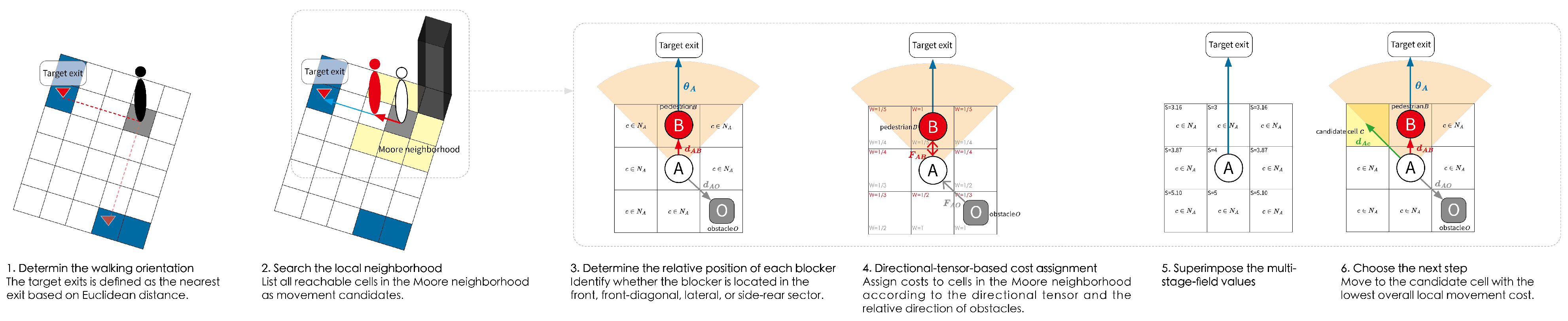
This study developed a direction-aware cellular automaton (CA) evacuation model for complex multi-room floor plans to analyze the effects of exit location on evacuation. The model includes three core modules and an accompanying evaluation framework (Figure 1): (1) a multi-stage static gradient field, which provides continuous and rational global guidance within hierarchical spatial structures; (2) an eight-neighborhood directional tensor, which improves directional consistency in local decisions on complex layouts; (3) dynamic neighborhood interference, which characterizes the obstructive effects of agents and obstacles on candidate movements; and (4) an integrated evaluation framework combining structure, behavior, time, and risk (density) to quantify exit location effects.
The building space was discretized into regular grid cells. Each cell recorded its static gradient value, neighborhood occupancy state, and exit assignment information. At each time step, each agent selected its movement direction by minimizing a local cost function, thereby coupling global path guidance with local avoidance.

2.1.2. Spatial Discretization

The building floor plan was discretized into square cells with a side length of Δ x = 0.4 m . Obstacle cells were non-walkable, whereas free cells were walkable. Exit cells were treated as boundary cells for the static field. Let P i j denote the cell located at row i and column j. Candidate moves were defined by the Moore neighborhood (eight neighborhoods), such that at each time step, an agent could move to at most one of the eight adjacent cells. The time step and speed calibration are described in Section 2.1.5.

2.1.3. Construction of the Multi-Stage Static Gradient Field

To represent hierarchical evacuation route relationships in complex floor plans more accurately, this study adopted a multi-stage static field construction strategy, so that the static field had a rational guidance direction within different functional regions and maintained a continuous transition at region boundaries.
Step 1: Baseline Field in the Main Region
Within the main region Ω main , for any free cell P i j , the baseline static field was defined as the minimum Euclidean distance to the exit set E:
S main ( P i j ) = min e E ( i i e ) 2 + ( j j e ) 2 ,
where ( i e , j e ) denotes the grid coordinates of exit e. This static field formed a continuous gradient in space, and its descending direction pointed to the nearest exit, providing baseline global guidance.
Step 2: Special Region Processing
For corridor or passage regions Ω s from which exits are directly visible, a local gradient field was constructed separately and used to override the static field in the main region. For any cell P i j in Ω s :
S s ( P i j ) = min e E ( i i e ) 2 + ( j j e ) 2 .
The special region was then eroded to obtain a boundary band for subsequent smooth merging:
B s = M s erode ( M s ) .
The static field within the special region was overlaid onto the global field:
S ( P i j ) = S s ( P i j ) , P i j M s .
Step 3: Smooth Blending
To avoid abrupt changes at the boundary between the main region and the special region, linear blending was performed within the boundary band. Let d ( P ) denote the distance from grid point P to the boundary of the special region, and let ω blend denote the width of the transition band (set to 10 grid units in this study). The blending coefficient was defined as
α ( P ) = d ( P ) ω blend .
The blended static field was written as
S ( P ) = S s ( P ) , P M s , α ( P ) S main ( P ) + ( 1 α ( P ) ) S s ( P b ) , 0 < d ( P ) < ω blend , S main ( P ) , otherwise ,
where P b denotes the corresponding point of P on the boundary. This step ensured a continuous change of the field at the regional transition, thereby reducing unrealistic direction switching caused by field discontinuities.
Step 4: Hierarchical Guidance for Small-Room Regions
For small-room regions Ω r such as offices and storage rooms, directly applying a unified distance field may easily lead to competing guidance directions that are inconsistent with guidance in the main region Ω main . Therefore, this study constructed an independent local field for each small room and superimposed a hierarchical offset so that agents preferentially leave the small space, merge into the main evacuation network, and then move toward exits along the main network.
For any cell P i j in a small room region, the field was defined as
S r ( P i j ) = min e E r ( i i e ) 2 + ( j j e ) 2 + G ref + δ ,
where E r denotes the set of exits for the room, G ref is the gradient value at the connection between the small-room region and the main evacuation network in Ω main , and δ is a constant offset (set to 10 in this study). This treatment established a hierarchical relationship between the small-room field S r and the static field in the main region S main , thereby reducing local misleading attraction and improving overall guidance consistency.

2.1.4. Eight-Neighborhood Directional Tensor and Dynamic Neighborhood Interference

At each discrete time step, agent A evaluated all accessible candidate cells c N A within its Moore neighborhood (unoccupied and non obstacle cells) and selected the next movement target by minimizing a local cost function:
C A ( c ) = α S ( c ) + β B N A ped I A , B ( c ) + γ O N A obs I A , O ( c ) ,
where S ( c ) denotes the static field value of candidate cell c, N A ped denotes the set of other agents within the neighborhood of A, I A , B ( c ) is the interference cost of agent B for agent A selecting candidate cell c, N A obs denotes the set of obstacles within the neighborhood of A, and I A , O ( c ) is the interference cost of obstacle O for agent A selecting candidate cell c. Parameters α , β , and γ are weighting coefficients. This formulation unified global guidance and local avoidance within the same decision framework.
Dynamic neighborhood interference was defined as the product of a physical repulsive strength and a directional weighting term to characterize the extent to which neighboring agents and obstacles hinder agent A when selecting a candidate move direction c:
I A , X ( c ) = F A , X W ( θ A , d A X , d A C ) , X N A ped N A obs ,
where F A , X describes the repulsive intensity exerted by agent B or obstacle O on agent A (denoted as F A , B when X = B and F A , O when X = O ). W ( · ) is a directional weighting function, reflecting directional sensitivity with stronger blocking in the front and weaker interference from lateral and rear directions.
The base repulsive intensity F A , X was defined with reference to the social force model and with consideration of agent geometric characteristics:
F A , B = k · exp S A + S B 2 l A B δ ,
F A , O = k · exp S A 2 + r obs l A O δ ,
where S A and S B denote shoulder widths (male: S = 0.495 m ; female: S = 0.457 m ), l A B and l A O are the Euclidean distances between agent A and agent B or obstacle O, r obs denotes the equivalent radius of the obstacle, and k and δ are parameters controlling the strength and range of the repulsive force.
The directional weighting function W ( · ) mapped the “target exit direction–relative orientation of neighboring pedestrians and obstacle–candidate move direction” into a discrete weight value, and it was implemented in a third-order tensor form. In this study, neighboring agent B and obstacle O in the neighborhood were evaluated using a unified directional sensitivity rule and were collectively referred to as the blocking source X. The directional weight was defined as
ω = W ( θ A , d A X , d A C ) , ω 1 , 1 2 , 1 3 , 1 4 , 1 5 ,
where θ A denotes the direction from agent A toward its target exit (determined by the local gradient of the static field) and was discretized into eight 45 sectors ( 0 , 45 , 90 , , 315 ) . d A X = ( d x X , d y X ) denotes the relative position direction of blocking source X with respect to agent A, and d A C = ( d x C , d y C ) denotes the displacement direction of candidate cell c with respect to agent A. Both vectors took values from the discrete eight-neighborhood direction set.
The weighting design followed the principle of “stronger influence in the front, weaker influence at the side and rear”. Using θ A as the reference, the influence of blocking source X relative to the candidate move direction d A C was classified into five levels, with stronger blocking corresponding to a larger weight. Specifically, the strongest, second-strongest, medium, weak, and weakest levels correspond to ω = 1 , ω = 1 / 2 , ω = 1 / 3 , ω = 1 / 4 , and ω = 1 / 5 , respectively. When θ A changed, the above partition rotated under the reference system of θ A so that the same neighborhood configuration yielded different interference evaluations under different moving directions, thereby improving the stability of direction selection in turning and high-density areas. The complete weighting tensor is provided in Appendix A, Figure A1. The agents’ decision-making logic is illustrated in Figure 2.

2.1.5. Update Strategy and Conflict Resolution

The model adopted a random sequential updating scheme. At each time step Δ t , all agents were randomly permuted and updated one by one, and their movements were computed and executed sequentially. If the target cell selected by an agent had already been occupied by another agent (or was an obstacle) at the moment of update, the agent remained at its current position in this time step. This treatment avoided systematic bias introduced by a fixed updating order.
The temporal scale was determined by calibrating the spatial step and the free walking speed. With grid size Δ x = 0.4 m and a free walking speed along axial directions (four neighborhood movement) of v 0 = 1.2 m s 1 , the time step was defined as
Δ t = Δ x v 0 = 0.4 1.2 0.333 s .
Since diagonal movement was permitted, the geometric displacement of a diagonal step was 2 Δ x , and thus the upper bound of the instantaneous speed was higher than the axial calibrated value. This setting was used to maintain the simplicity of discrete updating.

2.1.6. Parameter Setting and Calibration

The model parameters were grouped into three categories: (1) the weighting coefficients of the local cost function ( α , β , γ ) , (2) the repulsive strength parameters ( k , δ , r obs ) , and (3) the discrete value set of the directional weight tensor ω . To ensure that the model is reasonable at the macroscopic scale, the commercial evacuation software Pathfinder was used as a cross-model reference for consistency validation. Under the same building floor plan and initial conditions, the mean total evacuation time and its uncertainty range were compared. It should be emphasized that all parameters were fixed in advance before the validation, and the comparison was only used to verify macroscopic-level consistency and stability. No case-by-case parameter adjustment was performed across the five validation scenarios to reduce errors. The final parameter values adopted in this study are listed in Table 1.
The coefficients α , β , and γ are normalized weights used to balance the relative contributions of the static guidance term and the dynamic interference terms. Since the static field S ( c ) was not normalized (with values approximately in the range of 0–90), k was treated as a dimensionless scaling factor to match the magnitude of the static field term and the dynamic interference terms, thereby maintaining the modeling strategy of “static guidance dominance with dynamic interference correction”. When k = 10 , dynamic interference mainly acted under neighborhood conflicts and near obstacle conditions, without changing the overall global guidance direction. Parameter sensitivity analysis is provided in Appendix B.
The parameter settings in this study were mainly determined based on rule logic, cross-model comparison, and behavioral plausibility checks in order to support the comparative analysis of the mechanism through which exit location affects evacuation, rather than through strict inverse calibration using large-scale real-trajectory data. Therefore, the proposed model is more suitable as a tool for mechanism identification and relative comparison rather than as a fully empirically calibrated general predictive model.

2.2. Evaluation Metrics

2.2.1. Evacuation Efficiency

To compare overall evacuation performance under different exit layout scenarios, total evacuation time, percentile evacuation time, and tail indicators were used to jointly characterize evacuation efficiency and temporal structure.
The total evacuation time T total was defined as the time required from the start of evacuation until the last agent left the building.
The percentile evacuation time T p was defined as the time when the cumulative number of evacuated agents reached p % (in this study, p = 50 , 90 , 95 ), and it was used to describe characteristics of different stages of the evacuation process. To quantify the contribution of the late stage to the total evacuation time, the absolute tail time of the last ( 100 p ) % agents, T a i l p , and its proportion in the total time, T a i l R a t i o p , were defined as
T a i l p = T total T p .
T a i l R a t i o p = T total T p T total .
This study mainly reports results for p = 95 and p = 90 (i.e., the last 5% and the last 10% of agents) to identify whether changes in evacuation efficiency are mainly driven by the late-stage evacuation process.

2.2.2. Structural Fairness

Structural fairness was used to characterize the degree of balance of the theoretical service coverage of different exits under static gradient field guidance.
Service Area A i
The service area of exit i was defined as the total area of grid cells that were most inclined to move toward this exit under the guidance of the static gradient field:
A i = service _ area i .
A larger A i value indicates that the corresponding theoretical service coverage of the exit is wider. If A i differs substantially among exits, it indicates an evident bias in structural spatial partitioning.
Coefficient of Variation of Service Area C V A
The coefficient of variation of the service area was defined as
C V A = σ A A ¯ ,
where σ A is the standard deviation of { A i } , and A ¯ is the mean. C V A was used to measure the dispersion of the service area distribution, and a larger value indicates a more evident structural imbalance.
Gini Coefficient of Service Area G A
The Gini coefficient of the service area was defined as
G A = i = 1 E j = 1 E | A i A j | 2 E 2 A ¯ ,
where E denotes the number of exits. G A = 0 indicates that the service coverage of each exit is completely consistent, and a larger G A value indicates that the service coverage is more concentrated and the structure is more imbalanced.

2.2.3. Behavioral Fairness

Behavioral fairness was used to characterize the balance of actual evacuation flow allocation among exits.
Exit Utilization U i
The exit utilization of exit i was defined as
U i = evac _ count i N ,
where evac _ count i is the number of evacuated agents who chose exit i, and N is the total number of evacuated agents. U i reflects the proportion of evacuation flow actually borne by exit i.
Gini Coefficient of Exit Utilization G U
The Gini coefficient of exit utilization was defined as
G U = i = 1 E j = 1 E | U i U j | 2 E 2 U ¯ ,
where U ¯ is the mean of { U i } . G U = 0 indicates that evacuation flow is completely balanced among exits, and a larger G U value indicates that evacuation flow is more concentrated in a few exits.

2.2.4. Structure–Behavior Consistency

Comparing structural or behavioral indicators alone was insufficient to explain the causes of crowd splitting and congestion formation. Therefore, this study further compared the consistency between spatial service coverage and the actual utilization proportion.
Per Exit Deviation Δ i
For exit i, the per exit deviation was defined as
Δ i = U i service _ share i ,
where
service _ share i = A i e = 1 E A e .
Δ i = 0 indicates that the actual utilization proportion of exit i matches its spatial service coverage; Δ i > 0 indicates overutilization; and Δ i < 0 indicates underutilization. A larger | Δ i | value indicates weaker consistency between spatial partitioning and actual crowd splitting, and it usually implies that route convergence, local avoidance, or congestion feedback exert additional influence on crowd splitting.
Global Deviation Δ L 1
The global deviation Δ L 1 was defined as
Δ L 1 = i = 1 E | Δ i | ,
which represents the overall level of deviation across all exits. A larger Δ L 1 value indicates weaker structure–behavior consistency.
Global Deviation Δ L 2
The global deviation Δ L 2 was defined as
Δ L 2 = i = 1 E Δ i 2 ,
which is more sensitive to larger deviations occurring at a few exits and is suitable for characterizing the convergence or amplification of extreme imbalance.
Maximum Deviation Δ max
The maximum deviation Δ max was defined as
Δ max = max i | Δ i | ,
and it was used to highlight the deviation level of the most imbalanced exit.

2.2.5. Local Density Metrics

At each time step t, the mean density in region i was defined as
ρ i ( t ) = N i ( t ) A i ,
where N i ( t ) is the number of agents in region i at time t, A i is the region area, and the time step is Δ t = 1 / 3 s .
To characterize local risk, this study defined two types of indicators: peak intensity and duration. The peak density in region i in a single simulation run was defined as
ρ max , i = max t [ 0 , T ] ρ i ( t ) ,
where T is the total evacuation time of that run.
To avoid manually setting a fixed density threshold, a quantile-based adaptive threshold was adopted. For region i, given ρ max , i obtained from 50 simulation runs, the risk threshold was defined as
ρ thr , i = Q q ρ max , i ,
where Q q is the q th quantile, and this study used q = 0.9 .
The duration during which region i was in a high-risk state was defined as
D u r a t i o n i = t = 0 T 1 ρ i ( t ) > ρ thr , i Δ t ,
where 1 ( · ) is an indicator function that takes 1 when ρ i ( t ) exceeds the threshold and 0 otherwise.
To enhance the comparability of results across different scenarios, this study retains the quantile-based adaptive threshold while additionally introducing a fixed reference threshold, ρ ref = 1.0 person / m 2 , as a supplementary benchmark. This threshold is used primarily to represent high-density exposure states that are comparable across scenarios rather than as the unique normative boundary for risk assessment. Accordingly, the duration of high-density exposure can also be expressed as:
Duration i ref = t = 0 T 1 ρ i ( t ) > ρ ref Δ t ,

2.3. Controlled Experimental Design

2.3.1. Floor Plan and Initial Occupant Distribution

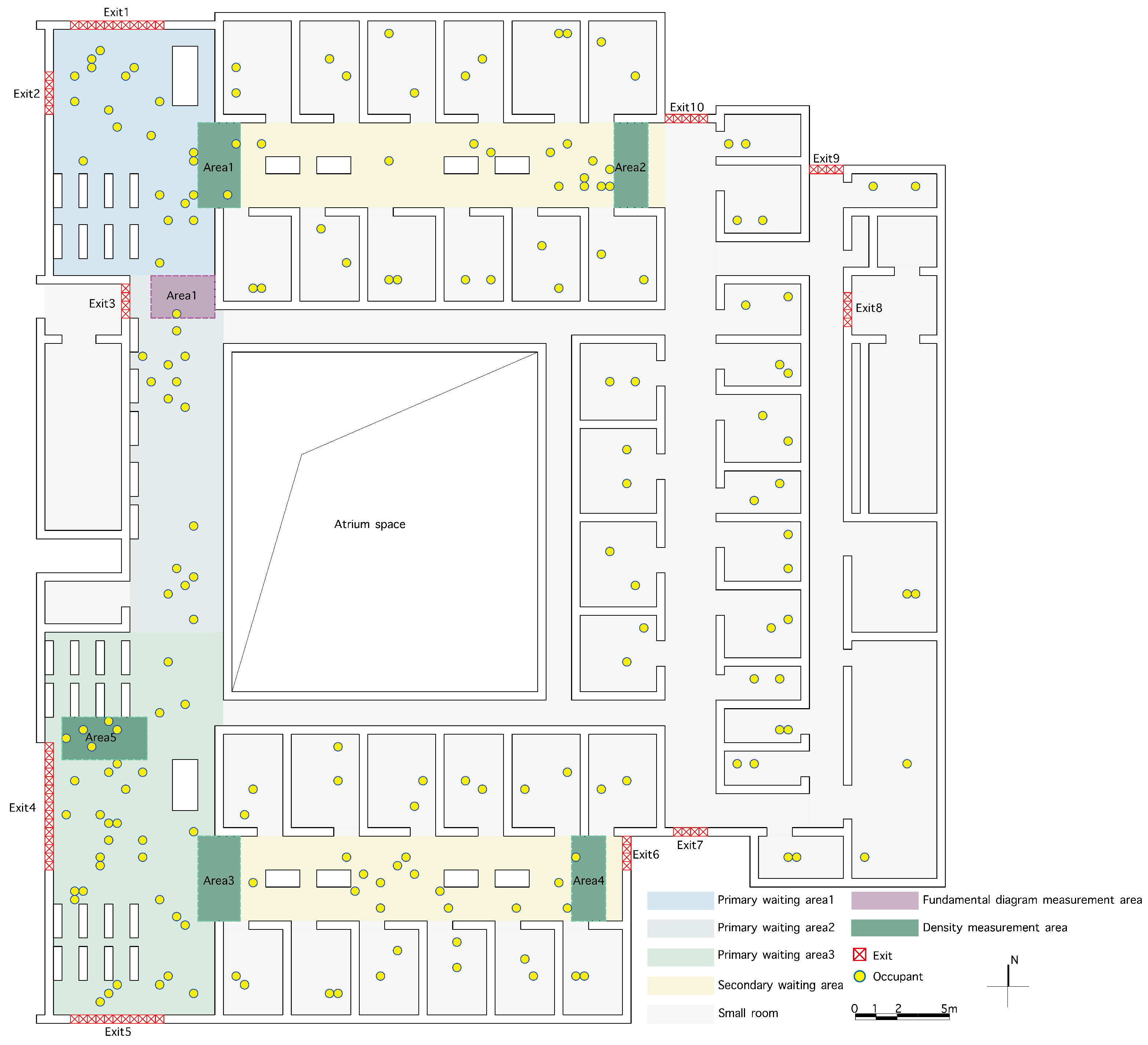
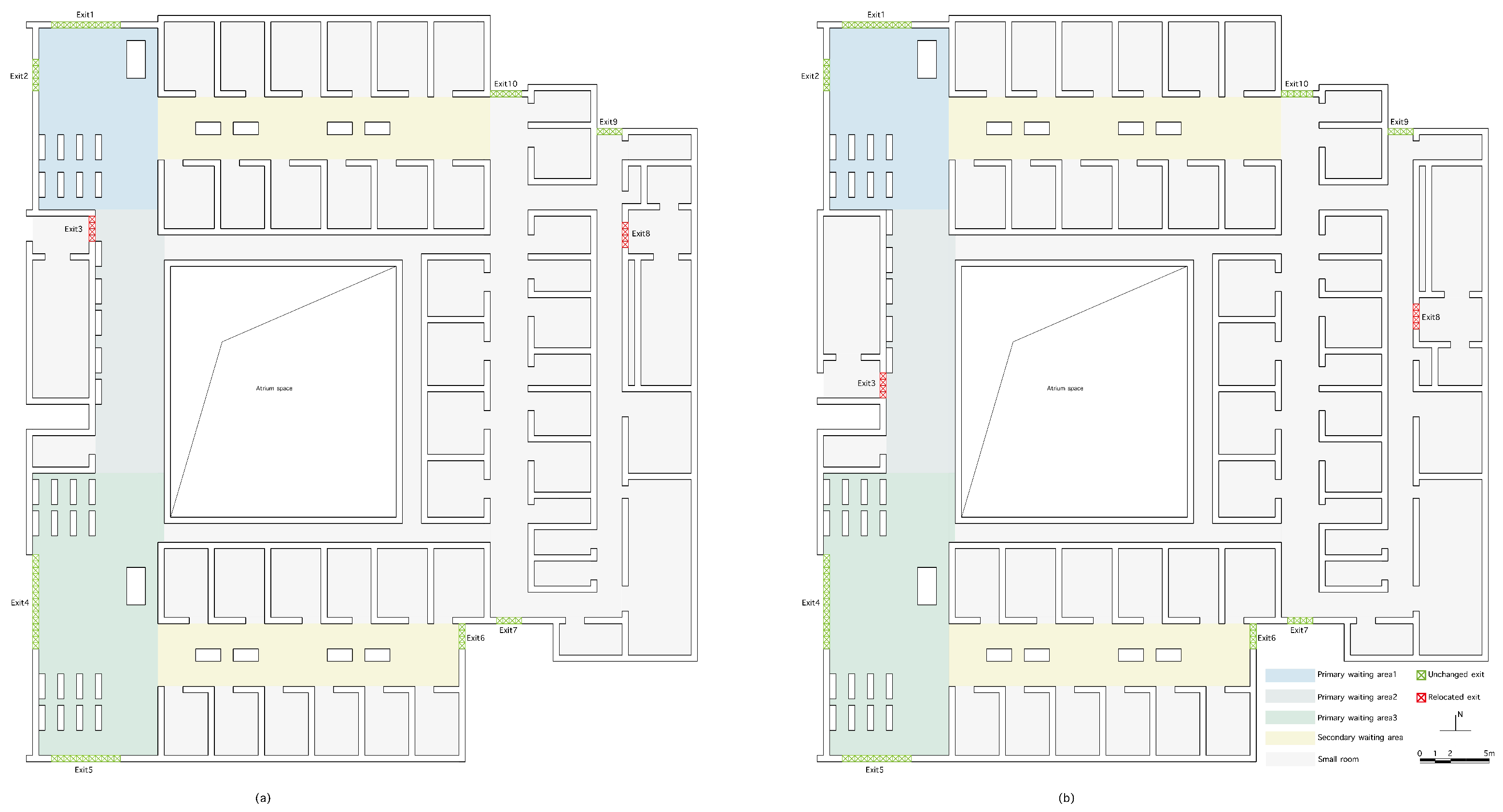
A hospital outpatient department was selected as the study case. Its floor plan has typical characteristics of complex multi-room buildings: multiple functional room units are connected by secondary corridors and further merge into a main corridor to form a hierarchical circulation network. The layout also includes multiple junctions and corners so that during evacuation, the flow undergoes a dynamic evolution from multi source inflow, to competition at nodes, to convergence along the main corridor, and finally to exit evacuation. Such spatial structures commonly face merging conflicts and tail evacuation in practical evacuation organization and thus can serve as a representative scenario for studying exit location effects in complex multi-room buildings. The study case covers typical functional spaces in the outpatient department, including the primary waiting area, secondary waiting area, consultation rooms, examination rooms, and physician offices, and includes 10 evacuation exits (Figure 3).
It should be noted that the purpose of this study was not to compare absolute evacuation performance across different types of building but to identify the exit location mechanism within a representative complex multi-room floor plan under strictly controlled conditions. Accordingly, the initial occupant distribution was set according to the functional zoning of the outpatient department (Figure 3) to reflect a typical situation of simultaneous evacuation from multiple rooms, and the two exit layout scenarios used exactly the same initial conditions to ensure comparability. Specifically, following the approximate proportions of function and area, 20, 15, and 35 occupants were randomly distributed in primary waiting areas 1, 2, and 3, respectively; 15 occupants were randomly distributed in each of the secondary waiting areas; and 2 occupants were randomly distributed in each small room, for a total of 186 occupants.

2.3.2. Exit Layout Scenarios and Controlled Variables

To examine the effect of exit location, this study adjusted the locations of Exit 3 and Exit 8 within the same building floor plan and constructed two exit layout scenarios for controlled comparison (Figure 4). The two scenarios remained consistent in exit number and exit width, building structure, obstacle distribution, occupant population and initial positions, and model parameters (including static field construction and local decision rules). Only the spatial exit locations differed, thereby isolating the independent effect of exit location changes on the evacuation process.
To evaluate fluctuations induced by stochastic mechanisms, each scenario was independently simulated 50 times to obtain statistically stable estimates. To justify the use of 50 repeated simulations for each scenario, the Monte Carlo estimation errors of two representative outcome indicators, T total and G U , were summarized in this study (see Appendix C). The comparison covered three aspects: evacuation efficiency, crowd splitting balance, and local risk. Evacuation efficiency is described in Section 2.2.1; the metrics of structural fairness, behavioral fairness, and structure–behavior consistency are described in Section 2.2.2, Section 2.2.3 and Section 2.2.4; the indicators of local density and risk duration are provided in Section 2.2.5; and the measurement area settings are introduced in Section 2.3.3.

2.3.3. Definition of Density Measurement Areas

Based on the building floor plan structure and evacuation route characteristics, five representative density measurement areas were selected for analysis (Figure 3). The selection followed three principles: (1) the areas were independent of exit location adjustment, and their locations were exactly the same in the two exit layout scenarios; (2) they were placed in functionally stable corridor locations, avoiding room interiors or areas with evident boundary effects; and (3) they covered key segments of the main corridor where convergence may occur during evacuation.

2.4. Validation Protocol

To validate the rationality of the proposed direction-aware cellular automaton (CA) model in spatial guidance, crowd splitting, and macroscopic evacuation efficiency, a three-level validation was conducted for two key modules, namely the multi-stage optimized static gradient field and the direction-aware eight-neighborhood directional tensor.

2.4.1. Static Gradient Field Guidance Consistency

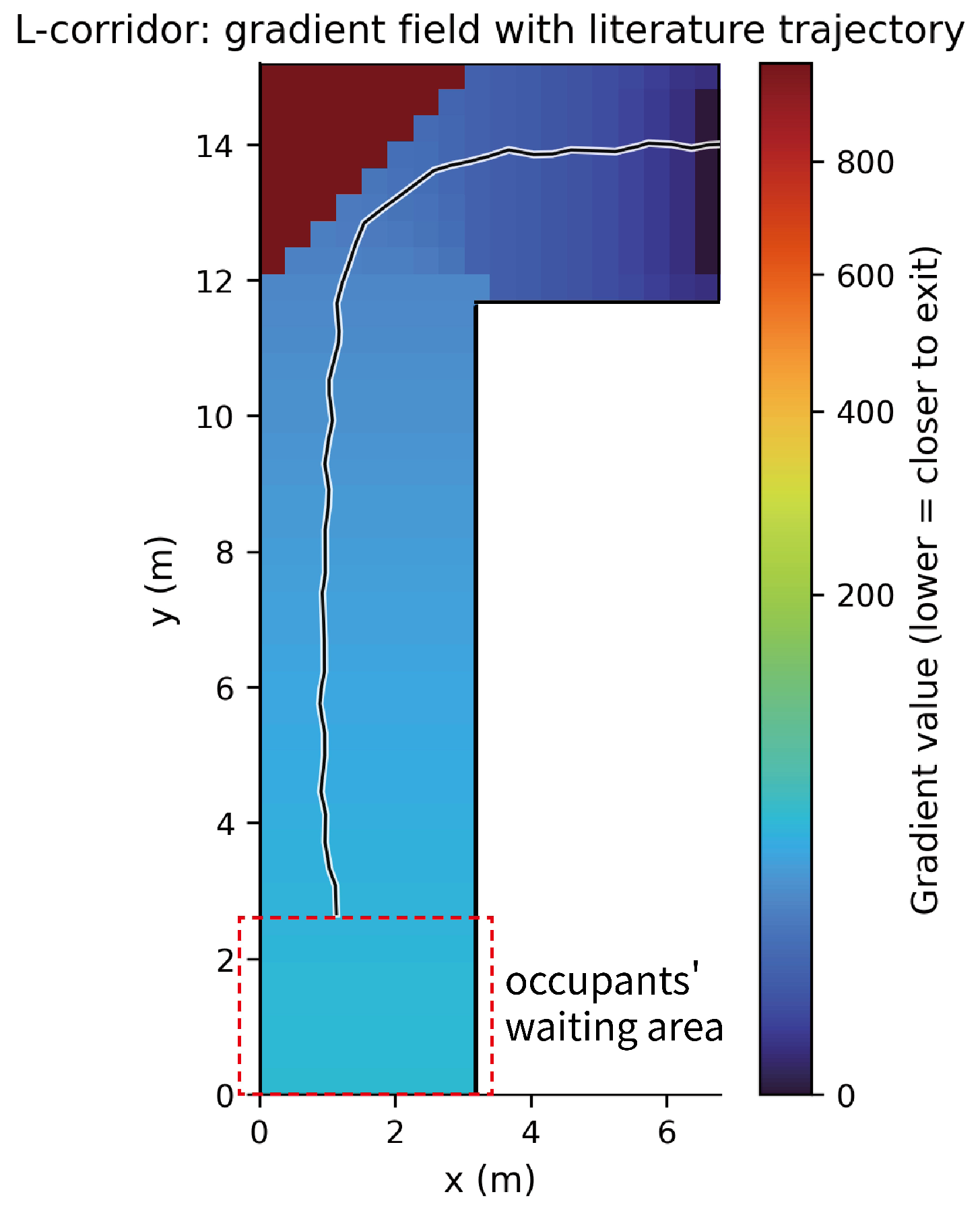
To examine the rationality of static gradient field guidance under a complex building floor plan, a published L-shaped corridor experiment was selected as the validation scenario [34]. To isolate the effect of the static gradient field, the directional tensor and the dynamic neighborhood interference modules were disabled, and only the movement tendency driven by the static field was retained. The corridor was discretized using the grid scale of this study and the static gradient field was generated, then overlaid and compared with the representative walking trajectories reported in the literature. Static field gradient values were sampled along the trajectories to examine the continuity of the gradient near the 90 corner and the guidance consistency of monotonic decrease toward the exit [34,35,36].

2.4.2. Macroscopic Consistency and Stability

To examine the macroscopic rationality of the directional tensor decision mechanism and the conflict resolution rule, the commercial evacuation software Pathfinder was used as a cross-model reference [37,38]. Five groups of the same building space and initial occupant distribution conditions were selected. Without changing the preset parameter settings of this study, the proposed CA model was independently repeated 100 times for each group (500 runs in total) to improve the stability of mean and confidence interval estimation, and Pathfinder outputs were used as a reference comparison. The comparison metrics included the mean total evacuation time and the 95% confidence interval, and the relative error was calculated. Normality tests and the results of parametric and non-parametric tests were used to assess whether systematic bias existed. It should be emphasized that this comparison aimed to examine whether macroscopic outputs were within an acceptable engineering consistency range and did not use Pathfinder results as a parameter-fitting target. To ensure comparability with the subsequent exit location analysis, the Pathfinder validation used the same building floor plan and grid discretization settings as the main experiments.

2.4.3. Fundamental Diagram Validation

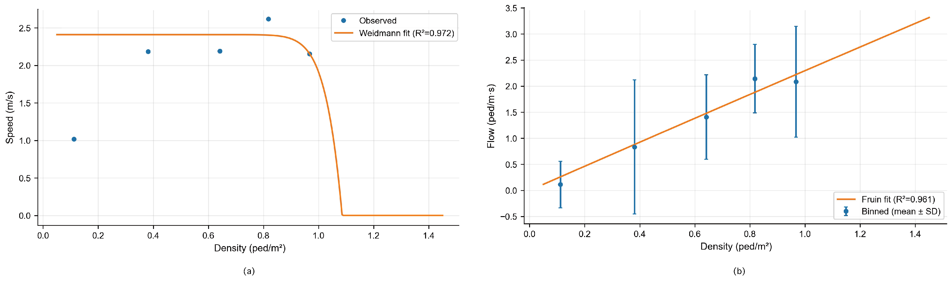
To verify whether the model reproduced classical pedestrian flow patterns at the local statistical level, a fixed fundamental diagram measurement area was set in the model (Figure 3). This area was placed in a straight corridor segment upstream of the exit and did not include exit boundary cells to reduce the influence of bottleneck boundary conditions on speed estimation. Local density, mean speed, and flow were calculated to construct density–speed and density–flow fundamental diagrams and fitted with the empirical models of Weidmann and Fruin. The evaluation metrics included R 2 , RMSE, and consistency in curve shape [39,40]. The free speed term was interpreted using an effective free speed definition to avoid the influence of discrete movement rules (including diagonal movement) on instantaneous speed estimation.

3. Results

3.1. Model Validation Results

Figure 5 shows the overlay of the static gradient field in the L-shaped corridor and the representative walking trajectories reported in the literature. Since this study used a 0.4 m grid discretization as a unified spatial reference, only rigid translation was applied to align the literature trajectories, without rotation or scaling. After alignment, nearest neighbor sampling of the static field gradient values was performed along the trajectory. The results show that the static field gradient value decreases significantly with increasing path length (Pearson r = 0.992 , p < 10 44 ; Spearman ρ = 1.000 , p < 10 78 ). This indicates that under the 0.4 m grid discretization, the constructed static gradient field can still provide directional guidance consistent with the experimentally observed main walking path in the turning region.
Table 2 presents the comparison results of total evacuation time between the proposed CA model and Pathfinder across five validation scenarios. Statistical tests indicate detectable differences between the two models, but the error magnitude in each scenario remained within an engineering acceptable range (the relative error threshold and equivalence judgment are given in Table 2), indicating that the two models have good macroscopic-level consistency. Based on this, we interpreted the comparison results as macroscopic agreement with controllable error, supporting the subsequent exit location analysis.
The density–speed relationship showed a monotonically decreasing trend. The Weidmann model fitting results were R 2 = 0.972 and RMSE = 0.128 . The density–flow relationship showed a standard unimodal structure. The Fruin model fitting results were R 2 = 0.961 and RMSE = 0.152 . The fitted curves are shown in Figure 6, and the corresponding fitting parameters and key characteristic values are summarized in Table 3.
Although the axial free walking speed in the basic model setting was specified as v 0 = 1.20 m / s , agents were allowed to move along diagonal directions under the discrete movement rules. Combined with the displacement-difference speed measurement adopted in this study, this leads to an “effective free-flow speed”, v 0 eff , that is higher than the axial preset value. It should be emphasized that v 0 eff only represents the kinematic characteristic of the model resulting from the combined effect of the discrete movement mechanism and the measurement protocol and does not correspond to the physiological free walking speed of real pedestrians. Therefore, in this part of the validation, v 0 eff is not treated as a direct estimate of real walking speed; instead, greater attention is paid to the consistency of the density–velocity and density–flow relationships in terms of curve shape, critical density, peak flow, and fitting indicators (e.g., R 2 and RMSE).
The sign test results in Table 2 indicate that, compared with Pathfinder, the CA model exhibits a slight but consistent tendency to produce longer evacuation times. This discrepancy may be related to differences in the spatial representation adopted by the two models. In the present study, space was discretized into 0.4 m grids, and individual motion was represented as discrete cell-to-cell transitions, whereas Pathfinder employs a continuous navigation logic that allows smoother local path adjustment. As a result, small delays associated with turning, obstacle avoidance, and bottleneck passage may accumulate gradually in the CA model. Given that this discrepancy remains within the predefined acceptable range, it is interpreted here as a conservative effect introduced by the discrete grid representation.
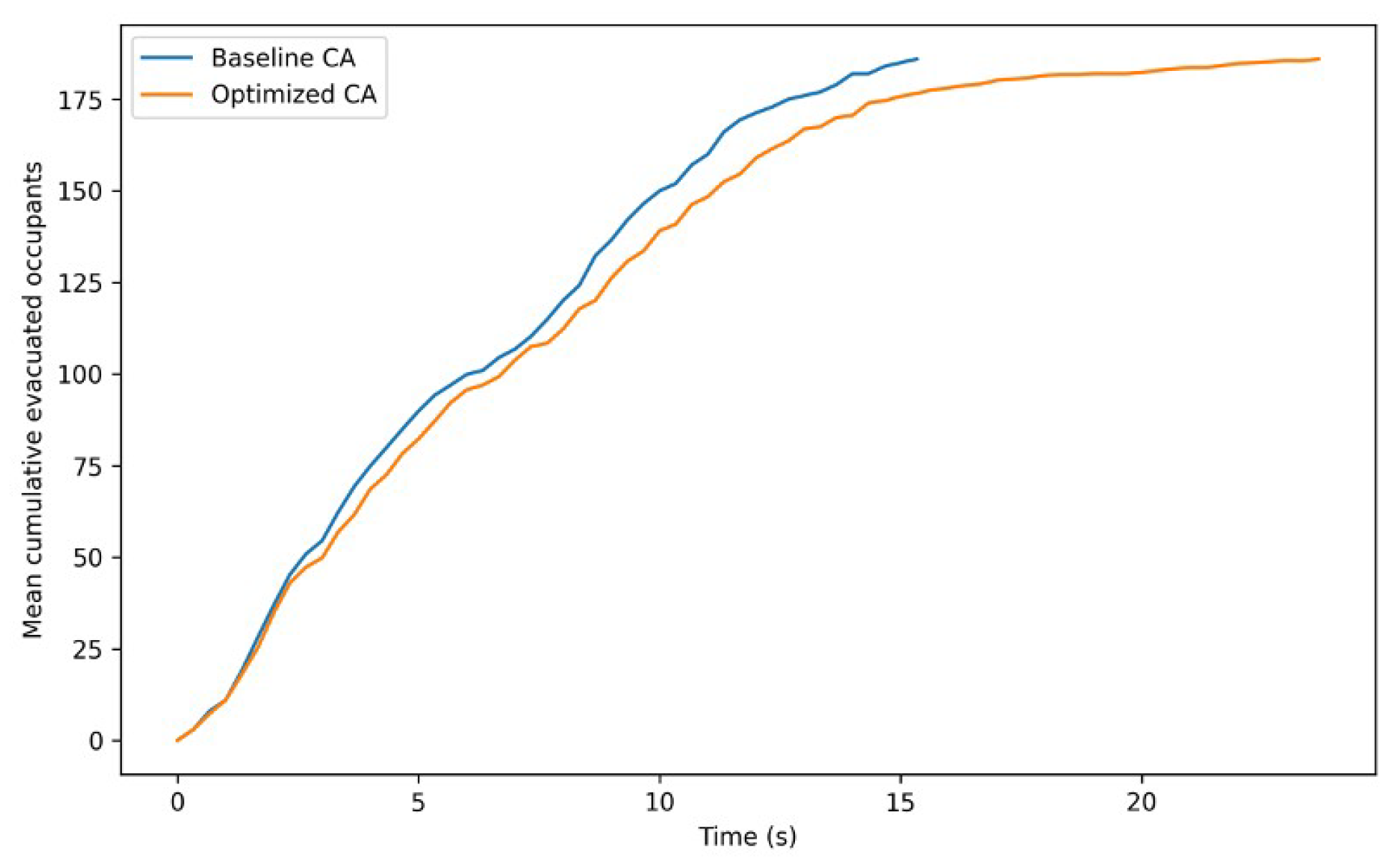
In addition, to illustrate the overall improvement of the proposed model relative to a simplified conventional CA, a baseline CA model based solely on the grid shortest-path static field was further constructed and analyzed under the same case setting. These results are not presented as part of the main text and are provided in Appendix D.

3.2. Comparison of Evacuation Efficiency

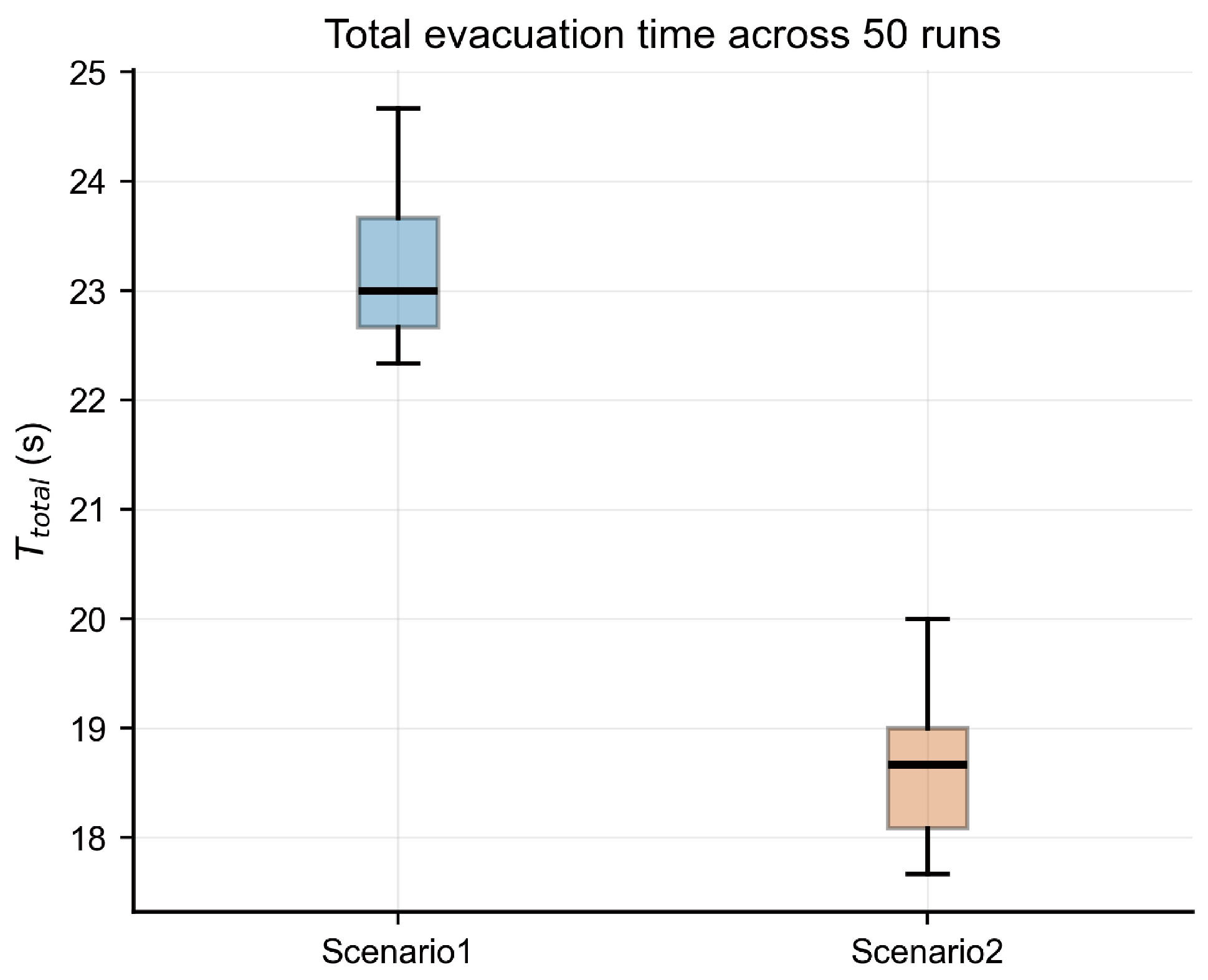
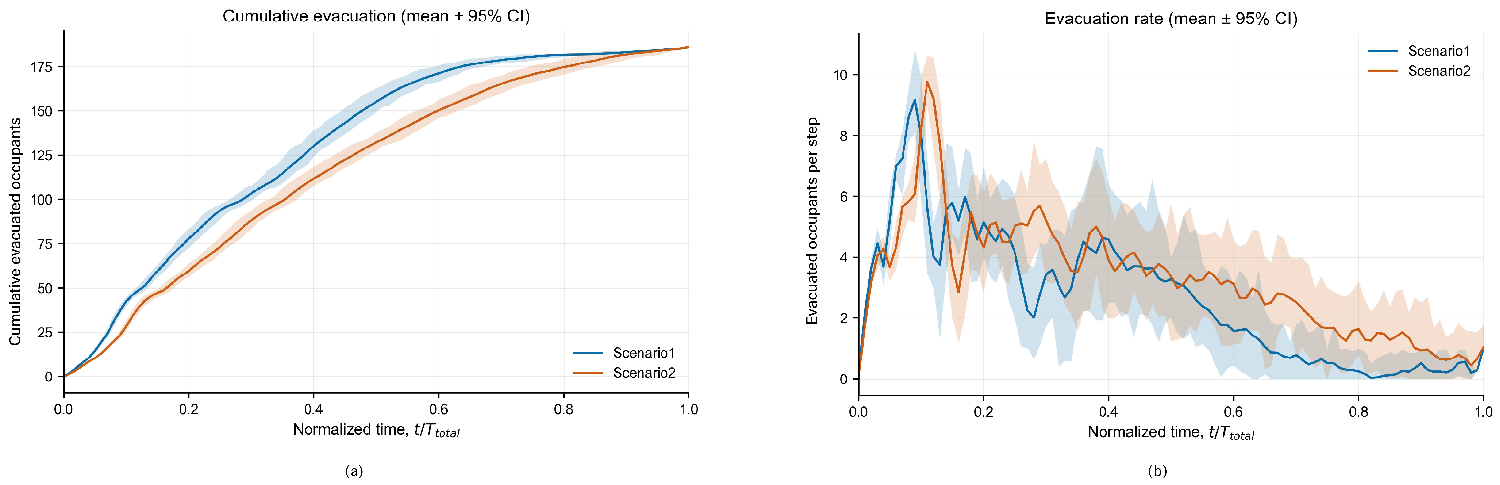
To evaluate the impact of exit location adjustment on overall evacuation efficiency, the total evacuation time ( T total ) from 50 simulation runs under each of the two layouts was statistically compared. The T total of Scenario 2 was significantly lower than that of Scenario 1 (approximately 20% reduction, Welch’s t test: p < 0.001 ) (Table 4 and Figure 7). The boxplot (Figure 8) also shows that the distribution of Scenario 2 was more concentrated, indicating that exit location adjustment improved efficiency while enhancing result stability.
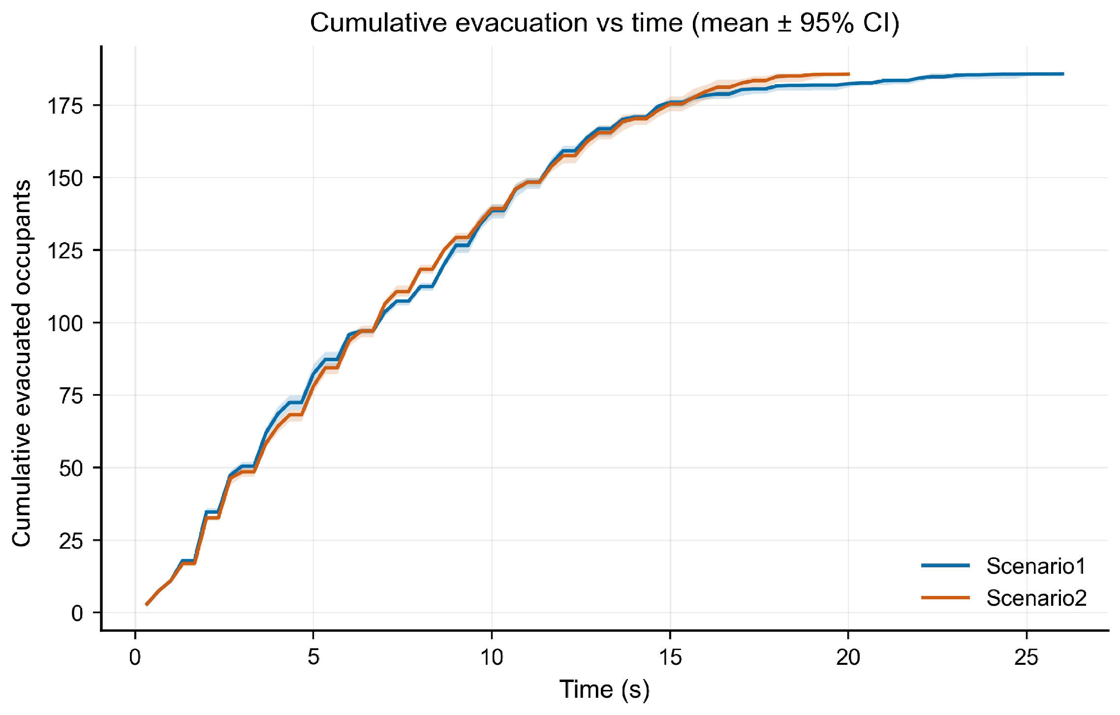
To identify the source of evacuation efficiency improvement, percentile evacuation times T 50 , T 90 , and T 95 were compared, as shown in Table 5. T 50 and T 90 in Scenario 2 increased slightly, and the change in T 95 was not significant. This indicates that the early and middle evacuation stage (0–95%) was not accelerated as a whole. Meanwhile, T total still decreased significantly, indicating that the improvement in evacuation efficiency originated from further acceleration of the evacuation process of the last 5% population (95–100%).
To address the limited descriptive power of p-values and confidence intervals with respect to the magnitude of differences, Hedges’ g effect sizes were further reported. The reduction in total evacuation time can be interpreted as an extremely large positive effect. By comparison, the quantile-based stage indicators exhibit heterogeneous changes: T 50 shows a relatively large negative effect ( g = 1.572 ), T 90 corresponds to a moderate negative effect ( g = 0.596 ), whereas the change in T 95 remains small ( g = 0.225 ).
Table 6 shows that T a i l 95 in Scenario 2 decreased significantly (approximately 60%), and T a i l R a t i o 95 decreased from 33.8% to 16.9%. The indicators T a i l 90 and T a i l R a t i o 90 for the last 10% population also decreased significantly. The duration of the 90–95% stage ( T 95 T 90 ) shortened slightly ( 4.85 % ), indicating that the late-stage tail structure showed a compression trend at multiple scales.
Combined with the cumulative evacuation curves (Figure 9), it could be further observed that the differences between the two layouts were limited in the early stage, whereas Scenario 2 showed a larger slope in the late stage, reflecting a higher evacuation speed of the tail crowd. Together with the percentile time and tail indicators, it can be confirmed that the improvement in evacuation efficiency caused by exit location adjustment was mainly dominated by the shortening of tail time in the late stage of evacuation, particularly for the last 5–10% population.

3.3. Behavioral Fairness

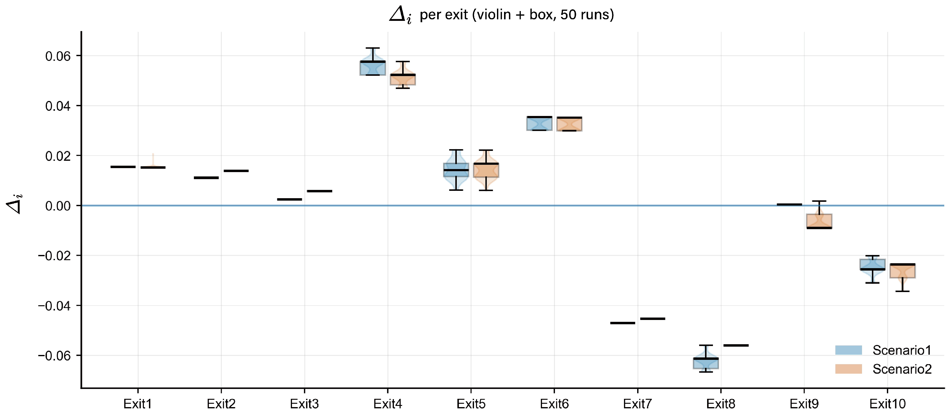
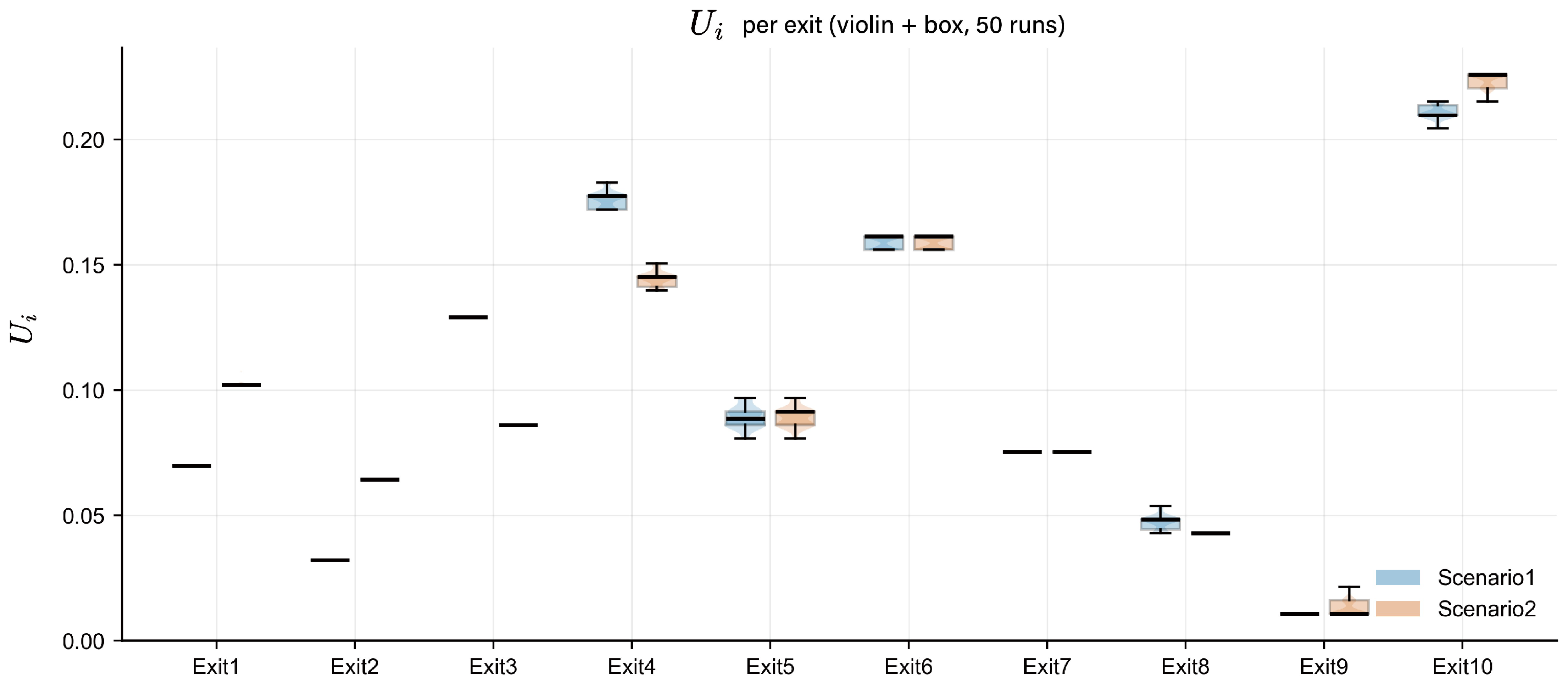
To evaluate the allocation balance at the behavioral level, the distribution of exit utilization U i across 50 simulation runs was analyzed. Figure 10 shows that in Scenario 1, exit utilization was evidently imbalanced, with some exits (such as Exit 4 and Exit 6) bearing evacuation loads significantly higher than the average level, while exits such as Exit 8 and Exit 9 had low utilization. In contrast, in Scenario 2, the utilization of some high-load exits decreased, while some originally low-utilization exits increased, and the utilization distribution tended to converge (complete U i results are provided in Appendix E, Table A9). However, based on the boxplot distribution, differences among exits still existed, indicating that layout adjustment affected evacuation behavior but did not completely eliminate behavioral imbalance.
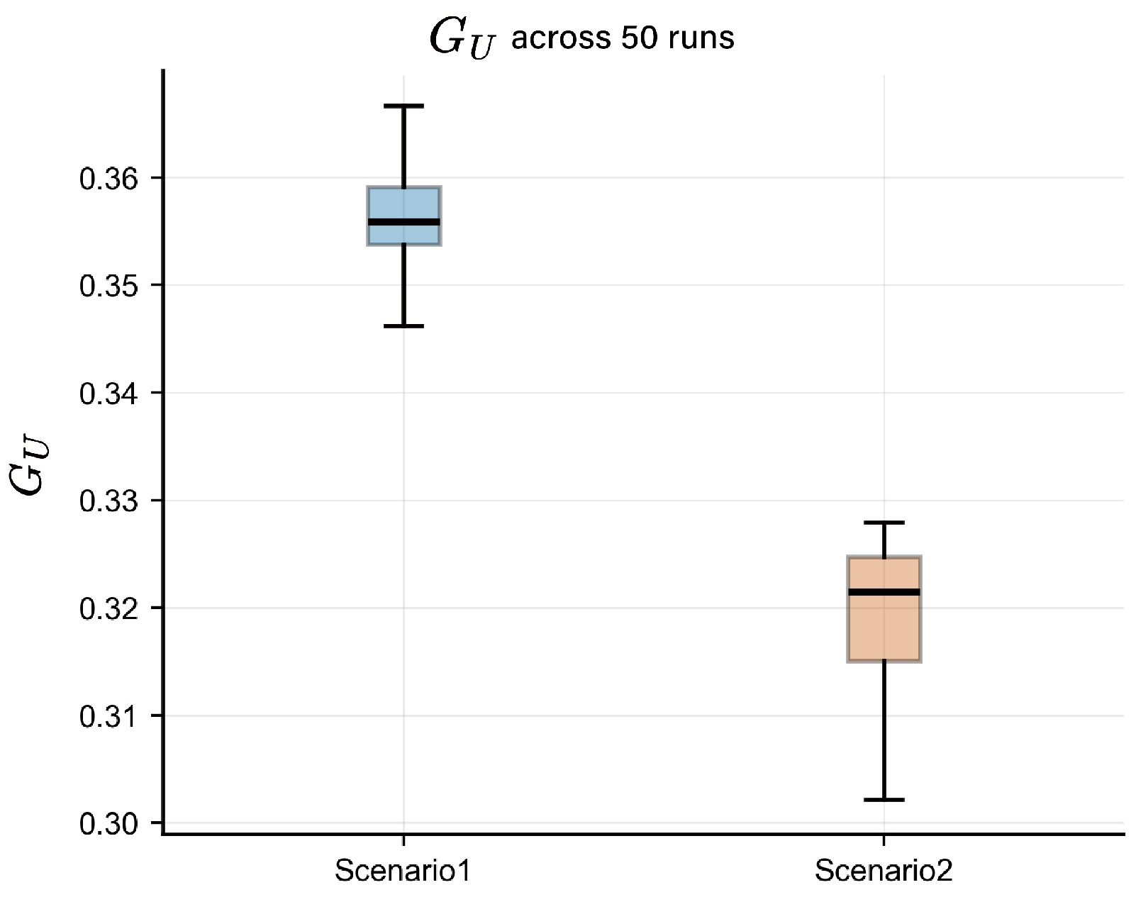
To further quantify the above differences, the Gini coefficient of exit utilization G U was calculated. The results show that G U decreased from 0.356 in Scenario 1 to 0.320 in Scenario 2, with a reduction of 10.09%, and the difference was highly significant (Welch’s t test, p < 0.001 ) (Table 7 and Figure 11). This result indicates that exit utilization in Scenario 2 was more balanced, and the degree to which utilization was concentrated in a small number of exits was significantly weakened.

3.4. Structural Fairness

To evaluate whether the attraction range of different exits in space was balanced, the service area A i of each exit and its proportional distribution were calculated. As shown in Table 8, in Scenario 1, the service area distribution across exits was evidently unbalanced. Some exits (such as Exit 10 and Exit 6) occupied a relatively large proportion of service area, while a few exits (such as Exit 9) had significantly smaller service areas, indicating that the static gradient field formed structurally dominant attraction zones and peripheral zones in space. In Scenario 2, the service area of some previously highly concentrated exits decreased, while the service area of some peripheral exits increased. This indicates that exit location adjustment can redistribute the partition boundaries of the static gradient field, making the spatial service coverage tend to be more balanced. However, the two layouts still retained similar partition pattern characteristics, indicating that exit location adjustment changed the areas assigned to exits but did not completely eliminate the tendency of structural concentration.
To quantify the dispersion of service areas, the coefficient of variation of service area C V A was calculated. As shown in Table 9, C V A in Scenario 2 decreased slightly, indicating that exit location adjustment reduced the dispersion of service areas to some extent and made the theoretical service coverage of exits more balanced. However, the change in C V A was limited, indicating that static field partitioning was still constrained by building spatial form and the structure of the route network, and the overall improvement in structural fairness was relatively limited.
Furthermore, the Gini coefficient of service areas G A was calculated. As shown in Table 9, G A 0.33 in Scenario 1, indicating a moderate level of structural concentration. G A in Scenario 2 decreased slightly, indicating that exit location adjustment weakened the concentrated structure of the static field and made the attraction domains of exits more balanced.

3.5. Structure–Behavior Coupling Relationship

To explain why exit location adjustment significantly changed evacuation efficiency under an unchanged number of exits, this study analyzed the results from the perspective of structure–behavior coupling. Under an ideal linear response condition, the actual utilization of a single exit should be approximately consistent with its service share, that is, U i service _ share i , corresponding to Δ i 0 . However, the results show that under both layouts, multiple exits had persistent positive deviations (overutilization) or negative deviations (underutilization) (Figure 12). The specific values are provided in Appendix E, Table A10. This indicates that actual crowd splitting did not simply correspond to service areas.
From the global consistency indicators, the effect of exit location adjustment was mainly reflected in alleviating extreme imbalance rather than in an overall decrease in the total deviation. Specifically, Δ L 1 did not differ significantly between the two layouts, whereas Δ L 2 and Δ m a x , which are more sensitive to extreme deviations, decreased significantly. Among them, Δ L 2 decreased by approximately 5.7% ( p < 0.001 ) (Table 10). This indicates that exit location adjustment reduced the dominance of a small number of key exits in evacuation tailing.
The exit-level results further revealed that the deviation was dominated by a small number of key exits. In Scenario 1, Exit 4 showed the most pronounced overutilization, while Exit 8 showed the most pronounced underutilization (Figure 12 and Appendix E, Table A10). In Scenario 2, the absolute values of these extreme deviations decreased significantly: the overutilization of Exit 4 decreased by 9.1%, and the underutilization of Exit 8 decreased by approximately 10%. Consistently, the changes in | Δ 4 | and | Δ 8 | also showed significant decreases. Therefore, exit location adjustment significantly weakened the structure behavior imbalance of over-concentrated exits and long-term underutilized exits. However, the deviations did not converge to zero as a whole but showed a pattern of partial reallocation of exit deviations. The positive deviations of Exit 2 and Exit 3 increased significantly, while Exit 9 shifted from a nearly matched state to a pronounced negative deviation (Appendix E, Table A10). These results indicate that exit location optimization did not simply eliminate all deviations, but, by changing the local decision environment and route convergence structure, it redistributed the extreme deviations previously concentrated on a few exits to more exits, thereby significantly reducing the dominance of key bottleneck exits in late-stage evacuation.
The shortening of total evacuation time and the significant decrease in behavioral level G U , together with the limited changes in structural fairness indicators ( C V A , G A ), indicate that the improvement in evacuation efficiency did not mainly originate from changes in service area distribution but was more closely related to changes in exit utilization distribution.

3.6. Local Density Analysis

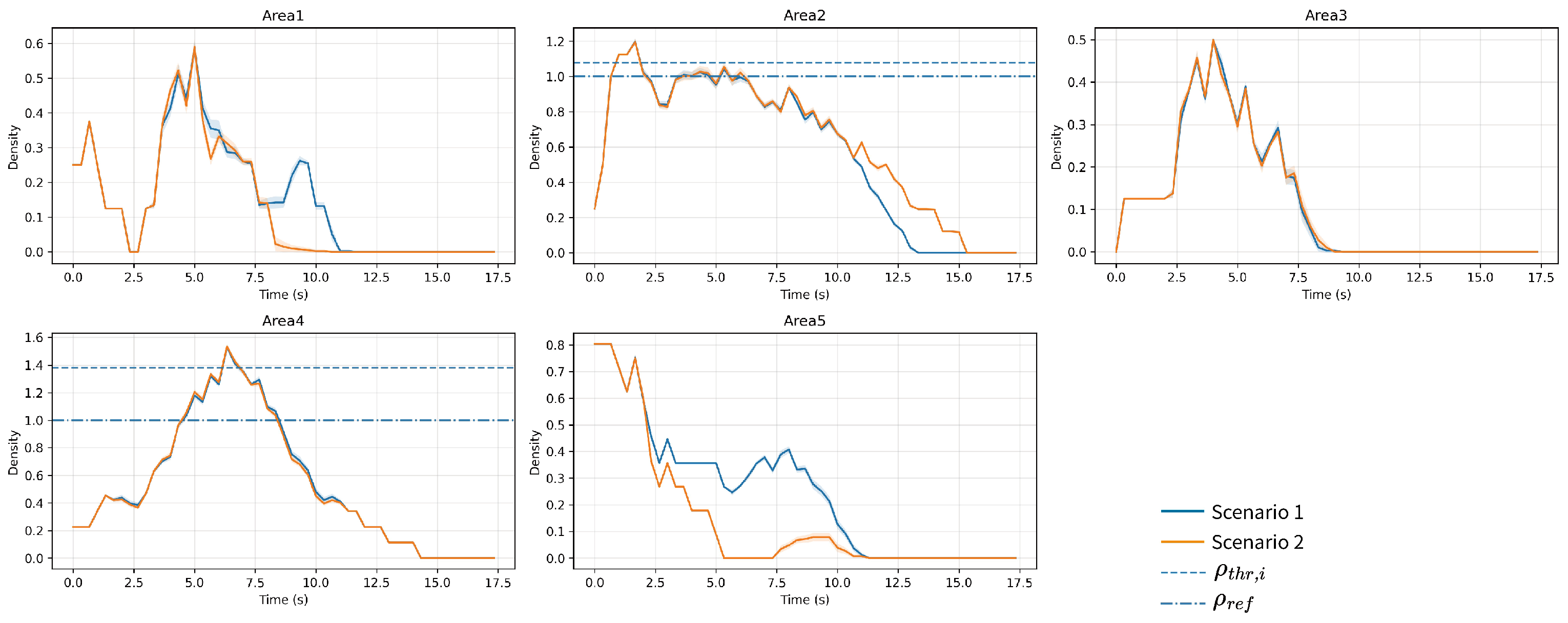
Figure 13 shows the statistical distribution of density evolution across 50 simulation runs. The density curves in each area showed a stable mean structure across repeated simulations, and the confidence intervals were overall narrow, indicating good statistical consistency of the results.
Table 11 summarizes ρ max , Duration i , and Duration i ref for the five measurement areas. In absolute terms, Area4 and Area2 exhibited the highest ρ max values, whereas Area1 and Area3 were relatively lower. However, between the two exit layouts, none of the regional ρ max differences reached statistical significance (all p > 0.5 ), and all effect sizes were small ( | g | 0.115 ). Under the Duration i metric, the duration values were generally low across all areas, with most being close to 0. In Scenario 2, the durations in Area2 and Area4 decreased from 0.007 s and 0.013 s to 0 s, respectively, but neither difference was statistically significant ( p = 0.322 ), and both effect sizes were small ( g = 0.198 ). Under the fixed-threshold metric Duration i ref , the durations in Area2 and Area4 were higher than those in the other areas, at approximately 1.83–1.98 s and 4.07–4.21 s, respectively. Among them, Area2 showed a slight increase in Scenario 2 ( p = 0.378 , g = 0.176 ), whereas Area4 showed a slight decrease ( p = 0.146 , g = 0.292 ), but neither reached statistical significance. The durations in the remaining areas under the fixed threshold were all close to 0.
Overall, the results under both threshold definitions consistently indicate that exit location adjustment did not lead to significant changes in either local peak density or the duration of high-density exposure.
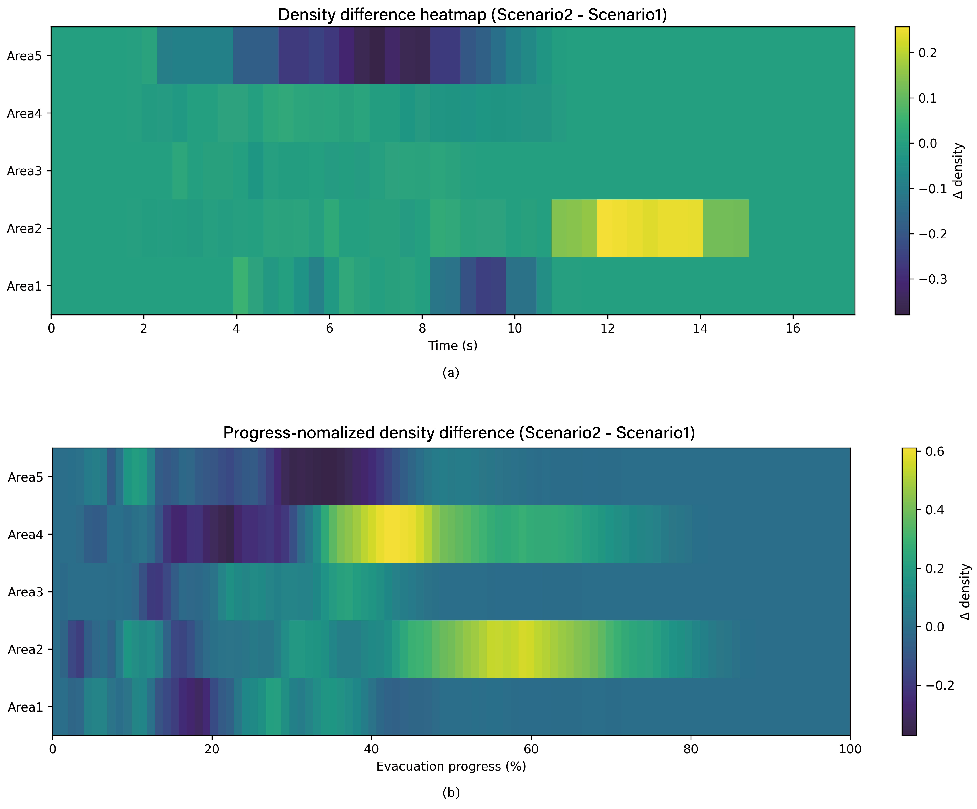
Figure 14 shows the density differences between the two layouts under the real time scale and the normalized evacuation progress scale. Under the real time scale, Area 2 showed a distinct positive difference interval at approximately 11–14 s, indicating that the local density in Scenario 2 was relatively higher during this stage. Area 1 and Area 5 showed short negative difference intervals in the early and middle stage, indicating that the local density in Scenario 2 was relatively lower during these stages. The difference magnitudes in Area 3 and Area 4 were overall small. Under the normalized progress scale, the same pattern was observed. During approximately 30–60% of the evacuation progress, Area 2 (and Area 4 in some stages) showed positive differences, while Area 1 and Area 5 showed short negative differences in the early stage; after the late stage (>80%), the differences tended to disappear. The consistent results across the two scales indicate that density differences mainly occurred in specific stages and were not persistent changes throughout the entire process.
Overall, the impact of exit layout adjustment on local density was mainly reflected in short-term fluctuations in specific stages.

4. Discussion

4.1. Mechanisms of Exit Location Effects

This study showed that, under unchanged exit number and exit width, total evacuation time could be significantly shortened by adjusting exit location in space (Figure 7 and Table 4). This is consistent with existing findings that exit location affects evacuation efficiency [41,42,43]. Previous studies have shown that exit choice behavior changes flow distribution and congestion structure, thereby affecting overall evacuation efficiency [44,45]. The present results further showed that the differences between the two layouts were limited in structural-level indicators, while the concentration of exit utilization at the behavioral level decreased markedly. This indicates that, compared with balancing structural service areas, the efficiency improvement was more likely related to the behavioral reallocation of exit utilization.
Changes in exit location first changed the spatial partitioning formed by the static gradient field, thereby affecting the initial route choice structure. On this basis, local decision rules such as direction awareness and neighborhood occupancy feedback further adjusted agent choices, strengthening or weakening the original crowd splitting structure, and finally leading to a reorganization of exit utilization. Therefore, the efficiency effect of exit location was essentially a reconfiguration effect of crowd splitting organization rather than an expansion of nominal capacity.
This finding indicates that, in complex multi-room buildings, the organization of crowd splitting explains evacuation efficiency differences better than nominal capacity.

4.2. Structure–Behavior Deviation

In theory, if occupants strictly follow the static field, exit utilization should be approximately consistent with its service share [46,47]. Under this assumption, crowd splitting organization can be regarded as a direct mapping of the building floor plan structure. However, the results of this study show that under both layouts, there was evident structure–behavior deviation, that is, exit utilization at the behavioral level did not linearly map to the building structure (Figure 12 and Table 10). This indicates that the actual crowd splitting outcome was not determined solely by floor plan partitioning. This is consistent with the conclusion of Wang Ke et al. (2022) that “evacuees may follow the mainstream of the surrounding environment, which may lead to deviations from the expected balance of exit use” [25].
The deviation arose from the adjustment of global guidance by local movement decision mechanisms. Direction-aware decisions mean that while following the global static gradient field, agents were also affected by neighborhood agents and thus changed movement direction. Such local feedback can produce nonlinear amplification or suppression effects on the original route choice [48,49,50], strengthening the utilization of some exits while weakening others. As a result, the behavioral distribution of exit utilization may deviate from the static field expectation induced by the building structure, forming structure–behavior deviation.
After exit location adjustment, structure–behavior deviation showed a convergence trend, indicating that exit location adjustment changed the local decision environment and thus regulated the deviation between building floor plan structure and behavior. In other words, structure–behavior deviation is not a fixed attribute but a dynamic outcome jointly influenced by floor plan partitioning and the decision mechanism.

4.3. The Critical Role of the Tail Evacuation Phase

Local density analysis showed that the differences in peak density in corridor areas were not significant between the two layouts, while the total evacuation time was significantly shortened (Figure 13 and Table 7). The cumulative evacuation curves showed that the efficiency improvement mainly appeared in the late stage of evacuation, that is, the evacuation process of the tail crowd was significantly compressed. This indicates that the efficiency improvement did not originate from reducing the maximum congestion intensity but was more reflected in changes in the temporal structure. This is consistent with Lan Qing et al. (2026), who concluded that ”because conflicts among pedestrians are smaller in the initial stage of evacuation, reducing the emphasis on avoiding congestion helps improve evacuation efficiency; because conflicts among pedestrians competing for positions intensify in the middle and late stage, placing more emphasis on avoiding congestion helps improve evacuation efficiency” [51].
Exit location adjustment reduced persistent queuing in front of specific exits by optimizing crowd splitting organization and the distribution of exit utilization across different evacuation stages, thereby shortening the residence time of the remaining population. The compression of the tail evacuation phase therefore reflects an optimization outcome of crowd splitting organization in the time dimension.
It should be noted that this optimization did not produce a uniform improvement throughout the entire evacuation process. The percentile evacuation time results (Table 5 and Table 6) show that T 50 and T 90 changed under the optimized scenario, whereas the variation in T 95 was limited. At the same time, the total evacuation time and the tail stage indicators improved significantly. This suggests that the benefit of exit location optimization is better understood as a redistribution of evacuation time across different stages, that is, a slight concession in local efficiency during the early and middle stages in exchange for a substantial compression of persistent queuing and tail end delay in the later stage.
From the perspectives of operational management and safety, such a stage-based trade-off appears acceptable in the context of the present study. For complex spaces such as hospital outpatient departments, if the optimization does not significantly increase local peak density while substantially shortening the total evacuation time and compressing the tail end stagnation stage, then it has positive implications for both overall evacuation completion efficiency and late-stage risk control. In other words, exit location optimization in this case behaves more like a ”tail-governance” strategy than a ”full process synchronous acceleration” strategy.
If speed heterogeneity is further introduced, especially when slower individuals such as older adults, children, or persons with limited mobility are considered, the tail stage may become further prolonged, because the final clearance process is more likely to be dominated by the combined effect of low-speed individuals and local bottlenecks. Under such conditions, the tail compression mechanism identified in this study may still hold directionally, but its magnitude and its redistribution pattern across different stages require further examination.
These results indicate that peak density is insufficient to explain the efficiency differences caused by exit location changes. In complex buildings, even when peak density levels are similar, overall evacuation efficiency can still be significantly improved by optimizing crowd splitting organization to shorten the tail duration. Therefore, evacuation performance assessment should be based on a comprehensive judgment combining multi-dimensional indicators.

4.4. Implications for Sustainable Building Safety Design

Within a sustainable building safety framework, evacuation optimization should not rely only on the “capacity expansion” approach, such as increasing exit number or enlarging exit width, but should also focus on optimizing crowd-splitting organization under fixed-capacity conditions. In this study, with exit number and exit width kept unchanged, a significant reduction in total evacuation time was obtained by adjusting exit location in space (approximately 20%, see Table 4), indicating that exit location can serve as a safety improvement strategy with low resource input and low physical intervention, providing a more implementable pathway for performance-based retrofitting of existing buildings. It should be noted that, in existing hospital buildings, exit relocation may still be constrained by practical factors such as the structural core, load-bearing components, fire compartmentation, and retrofit costs. Therefore, the term ”low intervention” in this study is used only in a relative sense, compared with more costly measures such as increasing the number of exits, widening exit openings, or reconfiguring the overall circulation pattern, rather than implying that this strategy can be implemented unconditionally in all existing buildings.
From the perspective of sustainability-oriented building safety design, the findings of this study are also relevant to dimensions associated with safety and distributional balance. Specifically, the improvement in efficiency mainly arises from a significant compression of the tail stage of evacuation. The tail phase usually corresponds to the most unfavorable local queuing conditions and is also the stage where individual differences are more easily amplified. Therefore, incorporating tail evacuation into evacuation efficiency evaluation not only helps explain why total time decreases but also helps identify and reduce the residence risk and high density exposure time of the last group in bottleneck areas, thereby improving safety equity within the evacuated population. Consistently, the behavioral fairness indicator showed a more balanced allocation of exit utilization, indicating that exit location optimization can weaken the crowd splitting pattern in which a small number of exits are under long-term high load.
From the perspective of resilience-oriented design in the presence of uncertain disturbances, the results of this study indicate that exit location optimization also showed an improvement in the structure–behavior coupling relationship. Although the change in the overall deviation Δ L 1 was limited, the global deviation Δ L 2 and the maximum deviation Δ m a x , which are more sensitive to extremely imbalanced exits, decreased significantly (see Appendix E), indicating that the optimized layout reduced the dominance of a small number of key exits in system performance and alleviated the imbalance pattern of over-reliance on specific exits, persistent queuing, and tail evacuation. Meanwhile, the uncertainty of total evacuation time also showed a decreasing trend (for example, the width of the 95% confidence interval decreased by about one third, see Table 4), indicating that this strategy not only improved evacuation efficiency but also enhanced the consistency and predictability of outcomes under repeated scenarios, which has direct implications for resilience design under uncertain disturbances.
At the methodological level, the proposed multi-dimensional evaluation framework of structure, behavior, time, and density integrated overall efficiency, structural fairness, behavioral fairness, structure–behavior deviation, and local density risk indicators into a unified quantitative system, enabling a shift from performance comparison to mechanism explanation and providing a systematic assessment tool for performance-based evacuation design in complex buildings. It should also be noted that the term ”fairness” in this study is used primarily in an operational and distributive sense, referring to the degree of balance in service area allocation and exit utilization distribution rather than directly corresponding to broader concepts such as social equity or spatial justice. The discussion of ”sustainable building safety” in this study is mainly grounded in the mechanistic evidence provided by quantitative indicators, including evacuation time, distributional balance, local density exposure, and result stability. These indicators can reflect several aspects related to safety, fairness, and resilience at the analytical level, but they do not constitute independent operational measurements of these dimensions. Therefore, the findings of this study are better understood as mechanistic support for sustainability-oriented safety design rather than as a direct validation of broader sustainability performance.

4.5. Model Limitations and Future Research Directions

This study was developed on the basis of a grid discretized model, and the behavioral parameters of individuals have not yet been systematically calibrated using large-scale measured trajectory data. Therefore, the proposed model is more suitable as a tool for mechanism identification and relative comparison between schemes, rather than as a general predictive model. In addition, the analysis in this study is limited to a single-floor complex hospital outpatient layout. Accordingly, the findings are better interpreted as mechanistic evidence derived from a specific case rather than as general conclusions applicable to all complex buildings. Different building types, spatial topologies, occupant compositions, and floor-organization patterns may all influence the actual effects of exit relocation and the stages at which these effects emerge. Future research may incorporate measured trajectory data for parameter calibration and further examine, across different layout types such as corridor-type, hall-type, and multi-story buildings, how variations in plan parameters including spatial hierarchy, corridor width, node organization, and relative exit positions affect the structure–behavior mechanisms identified in this study, thereby improving the generalizability of the conclusions.

5. Conclusions

In the complex single-floor hospital outpatient department case considered in this study, under unchanged exit number, exit width, and occupant population, we conducted a controlled comparison of the effects of exit location on evacuation performance in a complex multi-room building based on a direction-aware cellular automaton (CA) model, and we established an integrated evaluation framework combining structure, behavior, and time for mechanism interpretation.
The main conclusions are as follows:
  • Under unchanged nominal capacity, exit location adjustment significantly shortened the total evacuation time, indicating that improvement in evacuation performance does not necessarily rely on capacity expansion.
  • The change in structural fairness was limited, while behavioral fairness became more balanced, indicating that the efficiency improvement mainly originated from the behavioral reorganization of crowd splitting rather than simple balancing of static service coverage.
  • Differences in local peak density were overall not significant, but tail time in the tail evacuation phase was significantly compressed, indicating that the key benefit of exit location optimization was reflected in the reduction of persistent queuing and residence time in the late stage rather than a simple decrease in maximum congestion intensity.
  • Structure–behavior consistency analysis showed that extreme deviations were alleviated, indicating that exit location reduced the systemic pattern of imbalanced exit dominance and tail evacuation by weakening over-reliance on key exits and long-term underutilization.
In summary, in the hospital outpatient department case modeled in this study, exit location is not only a geometric parameter but also an important design variable influencing crowd splitting organization and overall evacuation performance. The results indicate that, under the condition that the existing number and width of exits remain unchanged, exit location optimization can serve as a low-intervention performance improvement strategy, providing a case-based quantitative analytical approach and a mechanistic explanatory basis for performance-based evacuation design and safety optimization in complex multi-room spaces. It should be noted that the safety, distributional balance, and result stability discussed in this study are mainly established through mechanistic links based on indicators such as evacuation time, exit utilization distribution, structure–behavior deviation, and local density exposure rather than representing a direct validation of broader sustainability performance. Meanwhile, the conclusions of this study are still primarily based on a single case, and their external validity remains to be further examined in other building types, heterogeneous populations, and multi-story spatial settings.

Author Contributions

Conceptualization, Y.Z. and Y.X.; methodology, Y.Z.; software, Y.X.; validation, Y.X.; formal analysis, Y.X.; investigation, Y.X.; resources, Y.Z.; data curation, Y.X.; writing—original draft preparation, Y.X.; writing—review and editing, Y.Z.; visualization, Y.X.; supervision, Y.Z.; project administration, Y.Z.; funding acquisition, Y.Z. All authors have read and agreed to the published version of the manuscript.

Funding

This research was funded by the General Project of the National Natural Science Foundation of China, grant number 52478010.

Institutional Review Board Statement

Not applicable.

Informed Consent Statement

Not applicable.

Data Availability Statement

The simulation data supporting the findings of this study are available from the corresponding author upon reasonable request.

Conflicts of Interest

The authors declare no conflicts of interest.

Abbreviations

The following abbreviations are used in this manuscript:
CACellular automaton
SFMSocial force model
C V A Coefficient of variation of service area
G A Gini coefficient of service area
U i Exit utilization of exit i
G U Gini coefficient of exit utilization

Appendix A. Directional Weight Tensor Illustration
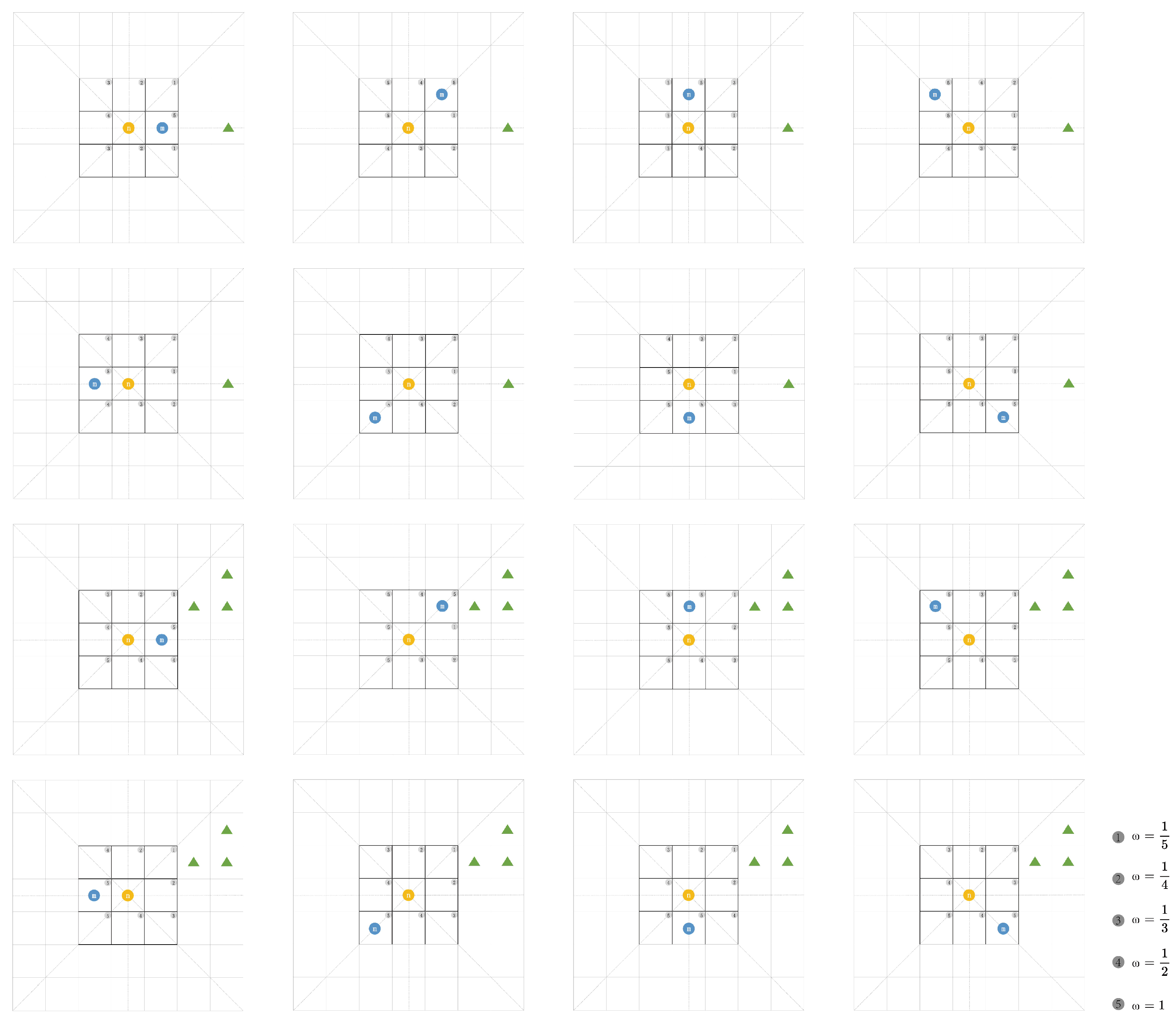
Figure A1. Directional weight tensor under the eight-neighborhood setting. Here, n denotes the agent, m denotes the obstacle source, and the green triangle indicates the exit.
Sustainability 18 03286 g0a1

Appendix B. Local Sensitivity Analysis of Key Weighting Parameters

To examine the influence of key weighting parameters on the main results, a local sensitivity analysis was conducted for α , β , γ , and k. For α , β , and γ , given the constraint α + β + γ = 1 , a one-factor-at-a-time perturbation scheme was adopted while keeping the total weight equal to 1. A total of seven parameter groups were defined, and each group was simulated 10 times under both the pre-optimization and post-optimization layouts. For k, while keeping α = 0.6 , β = 0.1 , and γ = 0.3 unchanged, three values, k = 8 , 10, and 12, were tested, with 10 repeated simulations conducted for each layout. This appendix reports only the three indicators directly related to the main conclusions, namely the total evacuation time T total , the tail-stage indicator T a i l 95 , and the Gini coefficient of exit utilization G U .
Table A1. Parameter settings for the sensitivity analysis.
Group α β γ Runs per Scenario
Base0.6000.1000.30010
α -low0.5000.1250.37510
α -high0.7000.0750.22510
β -low0.6330.0500.31710
β -high0.5670.1500.28310
γ -low0.6860.1140.20010
γ -high0.5140.0860.40010
Table A2. Sensitivity results of key indicators under the pre-optimization and post-optimization scenarios.
Group T total T a i l 95 G U
Scenario 1 Mean
(95% CI)
Scenario 2 Mean
(95% CI)
Scenario 1 Mean
(95% CI)
Scenario 2 Mean
(95% CI)
Scenario 1 Mean
(95% CI)
Scenario 2 Mean
(95% CI)
Base22.867 (22.565, 23.168)18.733 (18.109, 19.357)7.400 (7.067, 7.733)3.300 (2.804, 3.796)0.540 (0.533, 0.547)0.531 (0.522, 0.539)
α -low24.300 (22.803, 25.797)19.900 (19.171, 20.629)7.667 (6.341, 8.992)3.633 (2.859, 4.408)0.543 (0.531, 0.555)0.540 (0.533, 0.548)
α -high22.433 (22.237, 22.630)18.367 (17.834, 18.899)7.367 (7.191, 7.543)3.267 (2.685, 3.849)0.553 (0.546, 0.559)0.532 (0.524, 0.540)
β -low22.367 (22.291, 22.442)18.000 (18.000, 18.000)7.300 (7.225, 7.375)3.000 (3.000, 3.000)0.548 (0.538, 0.557)0.531 (0.515, 0.548)
β -high24.133 (23.386, 24.881)20.367 (19.464, 21.269)7.633 (6.683, 8.583)3.567 (3.063, 4.070)0.555 (0.543, 0.567)0.541 (0.535, 0.548)
γ -low24.767 (23.418, 26.116)19.200 (18.682, 19.718)8.500 (6.905, 10.095)3.367 (2.736, 3.997)0.551 (0.542, 0.560)0.531 (0.520, 0.543)
γ -high23.233 (22.513, 23.954)18.600 (18.126, 19.074)7.833 (7.103, 8.564)3.233 (2.730, 3.737)0.547 (0.540, 0.555)0.533 (0.526, 0.540)
Table A3. Percentage changes after optimization relative to the pre-optimization scenario.
Group Δ T total (%) Δ T a i l 95 (%) Δ G U (%)
Base−18.08−55.41−1.69
α -low−18.11−52.61−0.50
α -high−18.12−55.66−3.80
β -low−19.52−58.90−3.08
β -high−15.61−53.27−2.46
γ -low−22.47−60.39−3.57
γ -high−19.94−58.72−2.53
Table A4. Parameter settings for the k sensitivity analysis.
Group α β γ kRuns per Scenario
k-low0.6000.1000.300810
k-base0.6000.1000.3001010
k-high0.6000.1000.3001210
Table A5. Sensitivity results of key indicators under the pre-optimization and post-optimization scenarios for different k values.
Group T total T a i l 95 G U
Scenario 1 Mean
(95% CI)
Scenario 2 Mean
(95% CI)
Scenario 1 Mean
(95% CI)
Scenario 2 Mean
(95% CI)
Scenario 1 Mean
(95% CI)
Scenario 2 Mean
(95% CI)
k-low22.733 (22.463, 23.004)18.267 (17.974, 18.560)7.700 (7.393, 8.007)3.167 (2.757, 3.576)0.549 (0.539, 0.559)0.535 (0.529, 0.542)
k-base23.333 (23.109, 23.558)18.733 (18.347, 19.119)7.900 (7.544, 8.256)3.433 (3.012, 3.855)0.545 (0.537, 0.554)0.538 (0.527, 0.550)
k-high23.400 (22.863, 23.937)19.267 (18.549, 19.985)7.700 (7.156, 8.244)3.467 (2.809, 4.124)0.546 (0.538, 0.553)0.535 (0.526, 0.544)
Table A6. Relative changes after optimization compared with the pre-optimization scenario for different k values.
Group Δ T total (%) Δ T a i l 95 (%) Δ G U (%)
k-low−19.65−58.87−2.51
k-base−19.71−56.54−1.28
k-high−17.66−54.98−1.94
The results indicate that, within the tested parameter ranges, parameter perturbations led to limited fluctuations in absolute values, while the direction of the main conclusions remained stable. For α , β , and γ , Scenario 2 consistently exhibited lower T total and T a i l 95 values across all seven parameter groups, together with an overall reduction in G U . Specifically, the reduction in T total ranged from 15.61% to 22.47%, while the reduction in T a i l 95 ranged from 52.61% to 60.39%. For k, Scenario 2 likewise showed lower T total and T a i l 95 values across all three tested levels, with reductions of 17.66–19.71% for T total and 54.98–58.87% for T a i l 95 . Overall, the conclusion that “exit location optimization mainly improves overall evacuation performance by compressing the tail stage” demonstrates good parameter robustness.

Appendix C. Convergence of Repeated Simulations and Monte Carlo Error Assessment

To justify the use of 50 repeated simulations for each scenario, the stability of repeated results was examined from two aspects: first, the convergence of the cumulative means of the main outcome indicators; second, the Monte Carlo estimation error under 50 repetitions. The total evacuation time T total and the Gini coefficient of exit utilization G U were selected as representative indicators, reflecting overall evacuation efficiency and behavioral distributional balance, respectively.
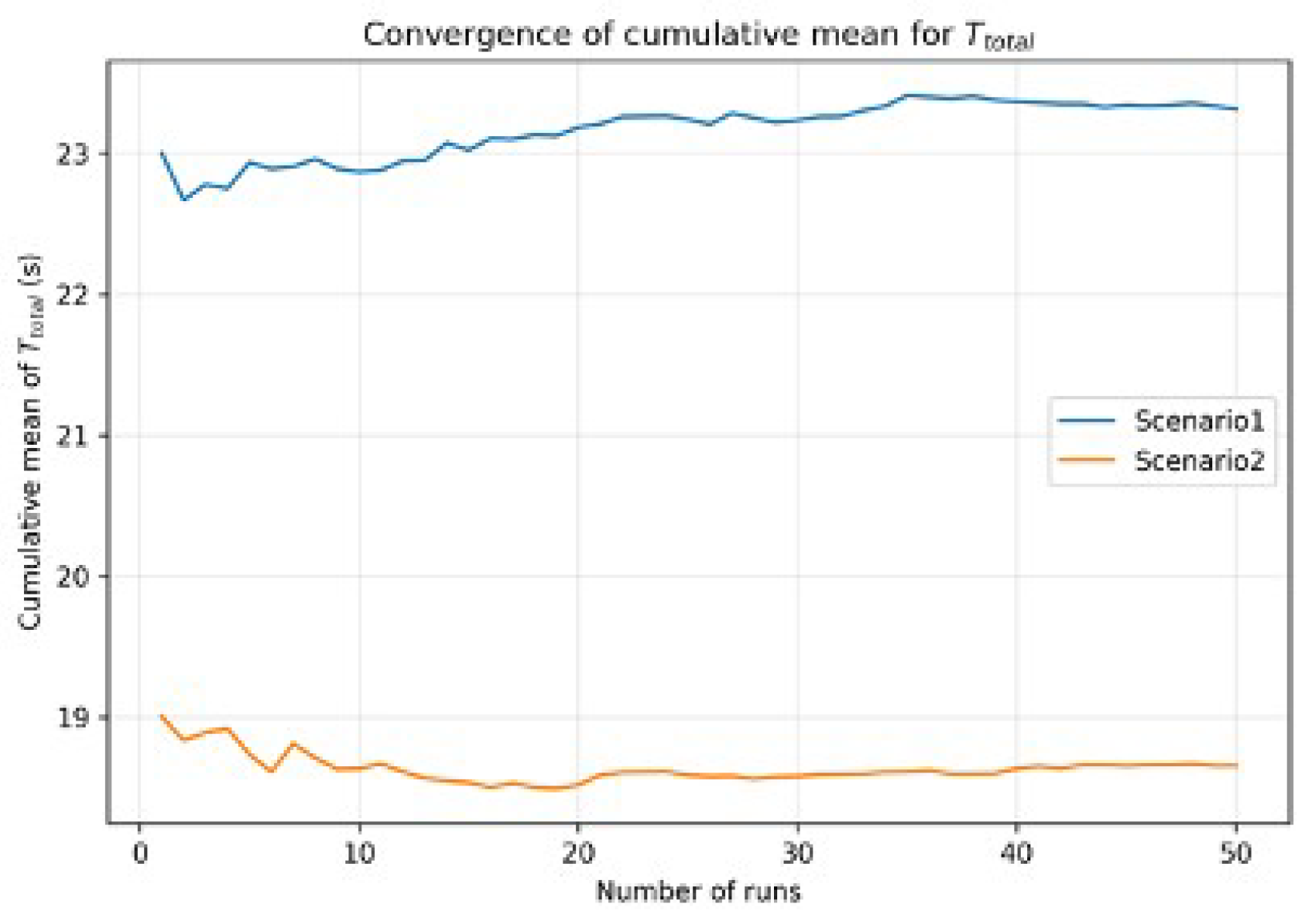
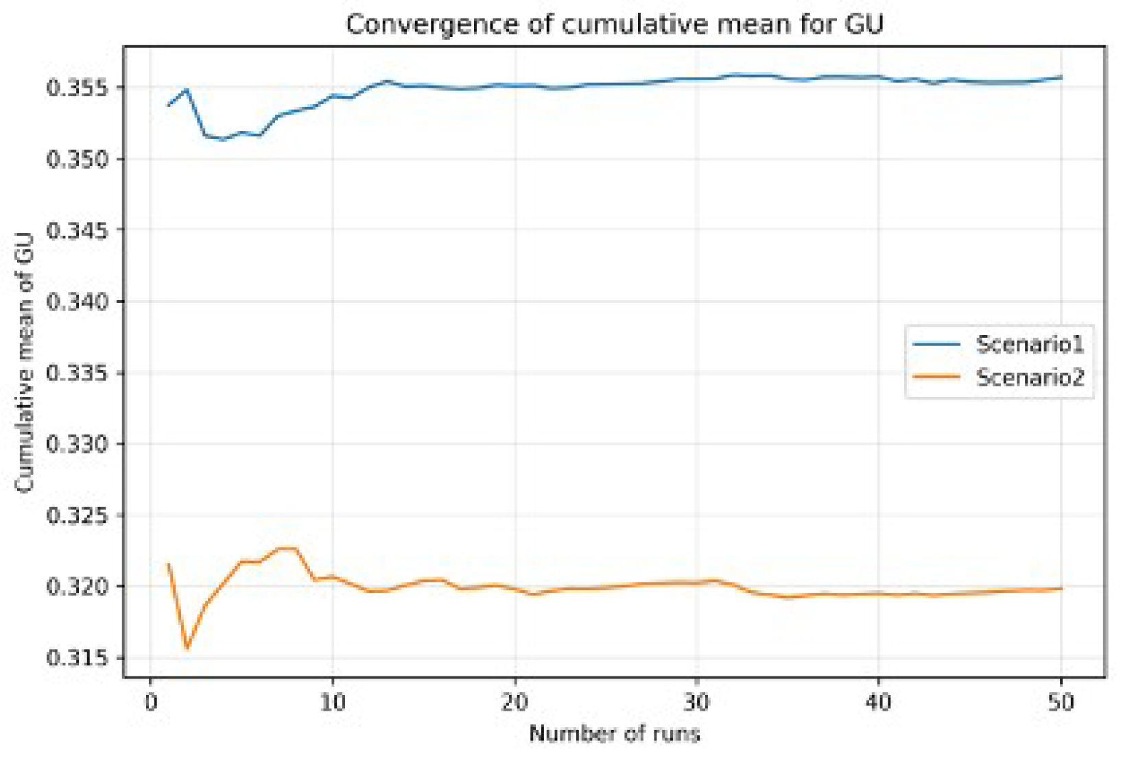
Figure A2 and Figure A3 present the evolution of the cumulative means of T total and G U as the number of simulation runs increases from 1 to 50. The results show that both indicators gradually converge as the number of repetitions increases, without evident late-stage drift, indicating that the main comparison metrics have reached a relatively stable state within the range of 40–50 runs.
Figure A2. Convergence of the cumulative mean for total evacuation time T total under the two scenarios.
Sustainability 18 03286 g0a2
Figure A3. Convergence of the cumulative mean for the utilization Gini coefficient (GU) under the two scenarios.
Sustainability 18 03286 g0a3
Table A7 further summarizes the Monte Carlo estimation errors under 50 repeated simulations. For T total , the cumulative means for Scenario 1 and Scenario 2 were 23.313 s and 18.653 s, respectively, with 95% confidence interval half-widths of 0.232 s and 0.154 s. For G U , the corresponding cumulative means were 0.3557 and 0.3198, with half-widths of 0.00147 and 0.00165, respectively. The relative half-widths for all indicators were below 1%, indicating that the remaining random estimation error after 50 repetitions was small. Therefore, 50 repeated simulations were considered sufficient to support the comparative analysis between scenarios.
Table A7. Monte Carlo estimation error at 50 runs for the representative outcome metrics.
MetricScenarioMean at 50 RunsSDSE95% CI Half-WidthRelative Half-Width (%)
T total Scenario 123.3130.8370.1180.2320.995
Scenario 218.6530.5550.0790.1540.825
G U Scenario 10.3560.0050.00080.0010.413
Scenario 20.3200.0060.00080.0020.516
SD: sample standard deviation; SE: standard error of the mean. 95% CI half-width = 1.96 × SE . Relative half-width (%) = ( CI half - width / mean ) × 100 .
It should be noted that 100 Pathfinder simulations were used in the validation stage mainly as a conservative choice for cross-model comparison. By contrast, 50 repetitions were adopted in the main experiments after confirming that the main indicators had reached sufficient stability. The two settings serve different analytical purposes and do not constitute a statistical inconsistency.

Appendix D. Baseline Model Comparison

To further illustrate the overall improvement of the proposed model relative to a simplified conventional CA, a baseline CA model was introduced for comparison. This baseline model retained only the grid-based shortest path static field toward the exits, without incorporating multi-stage static field construction, directional tensor constraints, or dynamic neighborhood interference. Its purpose was not to replace the proposed model but to serve as a low-complexity reference for comparing the overall changes in evacuation organization after the additional mechanisms were introduced.
The two models were independently simulated 10 times under the same building layout, identical exit settings, the same initial occupant number, and the same placement rules. Cumulative evacuation curves and overall indicators were then calculated using the same definitions as those adopted in the main text.
Figure A4 presents the mean cumulative evacuation curves of the two models. The results show that the simplified baseline CA rises faster in the early stage, exhibiting a stronger shortest-path directness. By contrast, the curve of the proposed optimized CA increases more gradually. This suggests that, in complex spaces, the combined effects of the multi-stage static field, directional constraints, and dynamic neighborhood interference alter both local step-selection behavior and the overall crowd splitting process.
Figure A4. Mean cumulative evacuation curves of the two models.
Sustainability 18 03286 g0a4
Table A8 shows that the baseline CA yields shorter T total and T a i l 95 values, whereas the two models produce nearly identical G U values. This indicates that the simplest baseline CA is closer to an idealized shortest path evacuation process and tends to underestimate detouring, delay, and local blocking effects in complex multi-room public spaces. By contrast, although the proposed model produces more conservative estimates of evacuation time, it is better able to represent behavioral constraints and environmental interference in complex spaces and is therefore more suitable for mechanism-oriented analysis.
Table A8. Comparison of overall indicators between the baseline CA and the optimized CA (10 runs).
MetricBaseline CA, Mean
(95% CI)
Optimized CA, Mean
(95% CI)
Relative Change of Optimized
CA vs. Baseline
T total (s)15.333 (15.333, 15.333)22.867 (22.258, 23.475)+49.13%
T a i l 95 (s)2.000 (2.000, 2.000)7.400 (7.077, 7.723)+270.00%
G U 0.541 (0.539, 0.544)0.540 (0.539, 0.541) 0.23 %
It should be emphasized that the baseline comparison in this appendix is intended to demonstrate the combined effect of the additional mechanisms rather than to isolate the independent contribution of each individual module. The main objective of this study remains the analysis of evacuation performance and mechanism differences before and after exit location adjustment under a unified modeling framework. The significance of the baseline comparison lies in showing that, if only a shortest path type CA is used, it is difficult to adequately capture crowd splitting reorganization and local interference in complex spaces, whereas the integrated model proposed in this study provides stronger explanatory power in this respect.

Appendix E. Supplementary Tables

Table A9. Exit utilization rates U i in Scenario 1 and Scenario 2.
MetricScenario 1 Mean (95% CI)Scenario 2 Mean (95% CI)Difference Mean (95% CI)
U 1 0.070 (0.070, 0.070)0.102 (0.102, 0.102)0.032 (0.032, 0.033)
U 2 0.032 (0.032, 0.032)0.065 (0.065, 0.065)0.032 (0.032, 0.032)
U 3 0.129 (0.129, 0.129)0.086 (0.086, 0.086) 0.043 ( 0.043 , 0.043 )
U 4 0.177 (0.176, 0.177)0.145 (0.144, 0.145) 0.032 ( 0.033 , 0.031 )
U 5 0.089 (0.088, 0.090)0.089 (0.088, 0.090)0.000 ( 0.002 , 0.002)
U 6 0.194 (0.193, 0.195)0.194 (0.193, 0.194) 0.000 ( 0.001 , 0.001)
U 7 0.106 (0.106, 0.106)0.105 (0.105, 0.105) 0.001 ( 0.001 , 0.001)
U 8 0.032 (0.032, 0.033)0.035 (0.035, 0.035)0.003 (0.002, 0.003)
U 9 0.100 (0.100, 0.100)0.093 (0.093, 0.093) 0.007 ( 0.007 , 0.007 )
U 10 0.210 (0.209, 0.211)0.209 (0.209, 0.209) 0.001 ( 0.002 , 0.000)
Table A10. Per-exit structure–behavior deviation Δ i and absolute deviation | Δ i | (mean and 95% CI) in Scenario 1 and Scenario 2, and their differences ( n = 50 ).
MetricScenario 1 Mean (95% CI)Scenario 2 Mean (95% CI)Difference Mean (95% CI)
Δ 1 0.015 (0.015, 0.015)0.015 (0.015, 0.016) 0.000 ( 0.000 , 0.000)
Δ 2 0.011 (0.011, 0.011)0.014 (0.014, 0.014)0.003 (0.003, 0.003)
Δ 3 0.002 (0.002, 0.002)0.006 (0.006, 0.006)0.003 (0.003, 0.003)
Δ 4 0.057 (0.056, 0.058)0.052 (0.051, 0.053) 0.005 ( 0.006 , 0.004 )
Δ 5 0.015 (0.013, 0.016)0.015 (0.014, 0.016) 0.000 ( 0.002 , 0.002)
Δ 6 0.033 (0.032, 0.034)0.033 (0.032, 0.033) 0.001 ( 0.001 , 0.001)
Δ 7 0.047 ( 0.047 , 0.047 ) 0.045 ( 0.045 , 0.045 )0.002 (0.002, 0.002)
Δ 8 0.062 ( 0.063 , 0.061 ) 0.056 ( 0.056 , 0.056 )0.006 (0.005, 0.007)
Δ 9 0.000 (0.000, 0.000) 0.007 ( 0.008 , 0.006 ) 0.008 ( 0.008 , 0.007 )
Δ 10 0.025 ( 0.026 , 0.024 ) 0.025 ( 0.026 , 0.025 ) 0.001 ( 0.002 , 0.000)
| Δ 1 | 0.015 (0.015, 0.015)0.015 (0.015, 0.016) 0.000 ( 0.000 , 0.000)
| Δ 2 | 0.011 (0.011, 0.011)0.014 (0.014, 0.014)0.003 (0.003, 0.003)
| Δ 3 | 0.002 (0.002, 0.002)0.006 (0.006, 0.006)0.003 (0.003, 0.003)
| Δ 4 | 0.057 (0.056, 0.058)0.052 (0.051, 0.053) 0.005 ( 0.006 , 0.004 )
| Δ 5 | 0.015 (0.013, 0.016)0.015 (0.014, 0.016) 0.000 ( 0.002 , 0.002)
| Δ 6 | 0.033 (0.032, 0.034)0.033 (0.032, 0.033) 0.001 ( 0.002 , 0.001)
| Δ 7 | 0.047 (0.047, 0.047)0.045 (0.045, 0.045) 0.002 ( 0.002 , 0.002 )
| Δ 8 | 0.062 (0.061, 0.063)0.056 (0.056, 0.056) 0.006 ( 0.007 , 0.005 )
| Δ 9 | 0.000 (0.000, 0.000)0.007 (0.007, 0.008)0.007 (0.006, 0.008)
| Δ 10 | 0.025 (0.024, 0.026)0.025 (0.025, 0.026)0.001 ( 0.000 , 0.002)

References

  1. Zhang, Z.; Ling, W.; Yang, Z.; Wei, X.; Wang, H. A congestion prediction model for optimizing emergency evacuation design of university libraries in China. J. Build. Eng. 2025, 99, 111537. [Google Scholar] [CrossRef]
  2. Cao, S.; Song, W.; Lv, W.; Fang, Z. A multi-grid model for pedestrian evacuation in a room without visibility. Phys. A Stat. Mech. Its Appl. 2015, 436, 45–61. [Google Scholar] [CrossRef]
  3. Xie, W.; Lee, E.W.M.; Li, T.; Shi, M.; Cao, R.; Zhang, Y. A study of group effects in pedestrian crowd evacuation: Experiments, modelling and simulation. Saf. Sci. 2021, 133, 105029. [Google Scholar] [CrossRef]
  4. You, L.; Wu, Q.; Wei, J.; Hu, J.; Wang, J.; Liang, Y. A study of pedestrian evacuation model of impatient queueing with cellular automata. Phys. Scr. 2020, 95, 95211. [Google Scholar] [CrossRef]
  5. Xie, D.F.; Gao, Z.Y.; Zhao, X.M.; Wang, D.Z.W. Agitated behavior and elastic characteristics of pedestrians in an alternative floor field model for pedestrian dynamics. Phys. A Stat. Mech. Its Appl. 2012, 391, 2390–2400. [Google Scholar] [CrossRef]
  6. Li, D.; Han, B. Behavioral effect on pedestrian evacuation simulation using cellular automata. Saf. Sci. 2015, 80, 41–55. [Google Scholar] [CrossRef]
  7. Najmanová, H.; Kuklík, L.; Pešková, V.; Bukáček, M.; Hrabák, P.; Vašata, D. Evacuation trials from a double-deck electric train unit: Experimental data and sensitivity analysis. Saf. Sci. 2022, 146, 105523. [Google Scholar] [CrossRef]
  8. Huan-Huan, T.; Li-Yun, D.; Yu, X. Influence of the exits’ configuration on evacuation process in a room without obstacle. Phys. A Stat. Mech. Its Appl. 2015, 420, 164–178. [Google Scholar] [CrossRef]
  9. Cai, Z.; Zhou, R.; Cui, Y.; Wang, Y.; Jiang, J. Influencing factors for exit selection in subway station evacuation. Tunn. Undergr. Space Technol. 2022, 125, 104498. [Google Scholar] [CrossRef]
  10. Ma, Y.; Chen, J.; Li, M.; Chen, Z.; Tong, Y.; Deng, Q.; Huo, F. Pedestrian Evacuation Simulation Considering Hiding Behavior and Obstacle Configurations Under Violent Attacks. Int. J. Disaster Risk Sci. 2025, 16, 1029–1043. [Google Scholar] [CrossRef]
  11. Li, Z.; Xu, W.A. Pedestrian evacuation within limited-space buildings based on different exit design schemes. Saf. Sci. 2020, 124, 104575. [Google Scholar] [CrossRef]
  12. Zhou, D.; Hu, J.; Gao, X.; Li, Z.; Wei, J.; Li, M.; Zhang, B.; Hu, Z. Queueing behaviors at exit in cellular automaton model with S-Queue. Int. J. Mod. Phys. B 2019, 33, 1950064. [Google Scholar] [CrossRef]
  13. Li, J.; Wang, J.; Li, J.; Wang, Z.; Wang, Y. Research on the influence of building convex exit on crowd evacuation and its design optimization. Build. Simul. 2022, 15, 669–684. [Google Scholar] [CrossRef]
  14. Cao, S.; Wang, M.; Zeng, G.; Li, X. Simulation of Crowd Evacuation in Subway Stations Under Flood Disasters. IEEE Trans. Intell. Transp. Syst. 2024, 25, 11858–11867. [Google Scholar] [CrossRef]
  15. Zhao, D.L.; Li, J.; Zhu, Y.; Zou, L. The application of a two-dimensional cellular automata random model to the performance-based design of building exit. Build. Environ. 2008, 43, 518–522. [Google Scholar] [CrossRef]
  16. Yu, H.; Li, X.; Song, W.; Li, J.; Song, X.; Zhang, J. A mixed crowd movement model incorporating chasing behavior. Simul. Model. Pract. Theory 2025, 138, 103044. [Google Scholar] [CrossRef]
  17. Wang, J.; Sarvi, M.; Ma, J.; Haghani, M.; Alhawsawi, A.; Chen, J.; Lin, P. A modified universal pedestrian motion model: Revisiting pedestrian simulation with bottlenecks. Build. Simul. 2022, 15, 631–644. [Google Scholar] [CrossRef]
  18. Zhu, Z.; Zhang, X.; Cao, J.; Sun, Y.; Zhou, X. An integrated model of crowd evacuation considering the coupling effects of temperature, density, and fall risk. Phys. A Stat. Mech. Its Appl. 2026, 682, 131169. [Google Scholar] [CrossRef]
  19. Kurdi, H.; Alzuhair, A.; Alotaibi, D.; Alsweed, H.; Almoqayyad, N.; Albaqami, R.; Althnian, A.; Alnabhan, N.; Islam, A.B.M.A.A. Crowd Evacuation in Hajj Stoning Area: Planning through Modeling and Simulation. Sustainability 2022, 14, 2278. [Google Scholar] [CrossRef]
  20. Zhao, X.; Huang, L.; Sun, Z.; Fan, X.; Zhang, M. Design Optimization of Building Exit Locations Based on Building Information Model and Ontology. Sustainability 2023, 15, 12922. [Google Scholar] [CrossRef]
  21. Ma, G.; Wang, Y.; Jiang, S. Optimization of Building Exit Layout: Combining Exit Decisions of Evacuees. Adv. Civ. Eng. 2021, 2021, 6622661. [Google Scholar] [CrossRef]
  22. Li, W.; Chen, Z.; Xu, J.; Wang, W.; Zhang, P. Research on evacuation simulation of underground commercial street based on reciprocal velocity obstacle model. J. Asian Archit. Build. Eng. 2022, 21, 22–33. [Google Scholar] [CrossRef]
  23. Yue, H.; Guan, H.; Shao, C.; Zhang, X. Simulation of pedestrian evacuation with asymmetrical exits layout. Phys. A Stat. Mech. Its Appl. 2011, 390, 198–207. [Google Scholar] [CrossRef]
  24. Shi, X.; Xue, S.; Feliciani, C.; Shiwakoti, N.; Lin, J.; Li, D.; Ye, Z. Verifying the applicability of a pedestrian simulation model to reproduce the effect of exit design on egress flow under normal and emergency conditions. Phys. A Stat. Mech. Its Appl. 2021, 562, 125347. [Google Scholar] [CrossRef]
  25. Wang, K.; Li, Y.; Qian, S. Analysis of Indoor Guided Pedestrian Evacuation Dynamics in Single- and Multiple-Exit Scenarios: Toward a Unified Scheme for Guide Assignment. Transp. Res. Rec. 2022, 2676, 632–647. [Google Scholar] [CrossRef]
  26. Huang, Y.; Yu, H.; Yang, Z.; Hu, X.; Pan, X. Emergency-Evacuation Safety Evaluation of Temporary Examination Rooms in University Teaching Buildings Based on Grey Relational Analysis. Appl. Sci. 2025, 16, 210. [Google Scholar] [CrossRef]
  27. Marzouk, M.; Mohamed, B. Integrated agent-based simulation and multi-criteria decision making approach for buildings evacuation evaluation. Saf. Sci. 2019, 112, 57–65. [Google Scholar] [CrossRef]
  28. Kunwar, B.; Simini, F.; Johansson, A. Evacuation time estimate for total pedestrian evacuation using a queuing network model and volunteered geographic information. Phys. Rev. E 2016, 93, 032311. [Google Scholar] [CrossRef]
  29. Kubicki, M.; Park, H. A New Method for Quantifying Exit Usage. Fire Technol. 2023, 59, 2179–2187. [Google Scholar] [CrossRef]
  30. Helbing, D.; Molnár, P. Social force model for pedestrian dynamics. Phys. Rev. E 1995, 51, 4282–4286. [Google Scholar] [CrossRef] [PubMed]
  31. Burstedde, C.; Klauck, K.; Schadschneider, A.; Zittartz, J. Simulation of pedestrian dynamics using a two-dimensional cellular automaton. Phys. A Stat. Mech. Its Appl. 2001, 295, 507–525. [Google Scholar] [CrossRef]
  32. Fu, Z.; Jia, Q.; Chen, J.; Ma, J.; Han, K.; Luo, L. A fine discrete field cellular automaton for pedestrian dynamics integrating pedestrian heterogeneity, anisotropy, and time-dependent characteristics. Transp. Res. Part C Emerg. Technol. 2018, 91, 37–61. [Google Scholar] [CrossRef]
  33. Lubaś, R.; Mycek, M.; Porzycki, J.; Wąs, J. Verification and Validation of Evacuation Models—Methodology Expansion Proposition. Transp. Res. Procedia 2014, 2, 715–723. [Google Scholar] [CrossRef]
  34. Xie, Q.; Wu, Y.; Wang, Y.; Zhang, H. A multi-grid evacuation model considering the effects of different turning types. Phys. A Stat. Mech. Its Appl. 2024, 635, 129497. [Google Scholar] [CrossRef]
  35. Xiong, X.; Luo, L.; Feng, Y.; Fu, Z.; Ma, J. Development of floor field cellular automaton model for pedestrian dynamics: Incorporating empirical acceleration mechanisms. Simul. Model. Pract. Theory 2025, 144, 103197. [Google Scholar] [CrossRef]
  36. Li, C.Y.; Li, X.H.; Chen, L. Modeling and simulation of pedestrian turning behavior at campus stair landings with retrograde movement. Phys. A Stat. Mech. Its Appl. 2025, 679, 131012. [Google Scholar] [CrossRef]
  37. Liu, J.; Zhang, R.; Yan, W.; Zhao, Q.; Guo, C. Modeling and simulation of fire evacuation considering guiding factors: A case study of Shenyang subway interchange station. Simul. Trans. Soc. Model. Simul. Int. 2024, 100, 1053–1068. [Google Scholar] [CrossRef]
  38. Chen, C.; Yu, R.; Wang, S.; Dai, Q. Modelling of crowd evacuation behavior considering the effects of drunken gait. Simul. Model. Pract. Theory 2025, 142, 103128. [Google Scholar] [CrossRef]
  39. Xing, S.; Wang, C.; Wang, W.; Cao, R.F.; Yuen, A.C.Y.; Lee, E.W.M.; Yeoh, G.H.; Chan, Q.N. A fine discrete floor field cellular automaton model with natural step length for pedestrian dynamics. Simul. Model. Pract. Theory 2024, 130, 102841. [Google Scholar] [CrossRef]
  40. Huo, F.; Deng, S.; Guo, C.; Ma, Y.; Zhang, W. Evacuation simulation considering pedestrian risk perception under toxic gas diffusion. Int. J. Disaster Risk Reduct. 2024, 109, 104589. [Google Scholar] [CrossRef]
  41. Wei, X.; Lou, Z.; Song, H.; Qin, H.; Yao, H. Exploring the Impacts of Exit Structures on Evacuation Efficiency. Fire 2023, 6, 462. [Google Scholar] [CrossRef]
  42. Kurdi, H.A.; Al-Megren, S.; Althunyan, R.; Almulifi, A. Effect of exit placement on evacuation plans. Eur. J. Oper. Res. 2018, 269, 749–759. [Google Scholar] [CrossRef]
  43. Fu, Z.; Yang, L.; Chen, Y.; Zhu, K.; Zhu, S. The effect of individual tendency on crowd evacuation efficiency under inhomogeneous exit attraction using a static field modified FFCA model. Phys. A Stat. Mech. Its Appl. 2013, 392, 6090–6099. [Google Scholar] [CrossRef]
  44. Chen, L.; Guo, Z.L.; Wang, T.; Li, C.Y.; Tang, T.Q. An evacuation guidance model for heterogeneous populations in large-scale pedestrian facilities with multiple exits. Phys. A Stat. Mech. Its Appl. 2023, 620, 128740. [Google Scholar] [CrossRef]
  45. Helbing, D.; Farkas, I.; Vicsek, T. Simulating dynamical features of escape panic. Nature 2000, 407, 487–490. [Google Scholar] [CrossRef]
  46. Kirchner, A.; Schadschneider, A. Simulation of evacuation processes using a bionics-inspired cellular automaton model for pedestrian dynamics. Phys. A Stat. Mech. Its Appl. 2002, 312, 260–276. [Google Scholar] [CrossRef]
  47. Li, Y.; Chen, M.; Dou, Z.; Zheng, X.; Cheng, Y.; Mebarki, A. A review of cellular automata models for crowd evacuation. Phys. A Stat. Mech. Its Appl. 2019, 526, 120752. [Google Scholar] [CrossRef]
  48. Guo, R.Y.; Huang, H.J.; Wong, S.C. A potential field approach to the modeling of route choice in pedestrian evacuation. J. Stat. Mech. Theory Exp. 2013, 2013, P02010. [Google Scholar] [CrossRef]
  49. Wu, P.Y.; Ge, Y.E.; Ma, Z.; Guo, R.Y. Modeling proactive avoidance behaviors in pedestrian flows considering congestion anticipation. Transp. Res. Part C Emerg. Technol. 2026, 184, 105532. [Google Scholar] [CrossRef]
  50. Ma, J.; Song, W.g.; Zhang, J.; Lo, S.m.; Liao, G.x. k-Nearest-Neighbor interaction induced self-organized pedestrian counter flow. Phys. A Stat. Mech. Its Appl. 2010, 389, 2101–2117. [Google Scholar] [CrossRef]
  51. Lan, Q.; Hu, J.; Fan, L.; Yang, L.; Zhang, Q.; You, L.; Wei, J.; Li, M. A pedestrian evacuation model with variable neighborhood simulated annealing. Int. J. Mod. Phys. C 2026, 37, 2550069. [Google Scholar] [CrossRef]
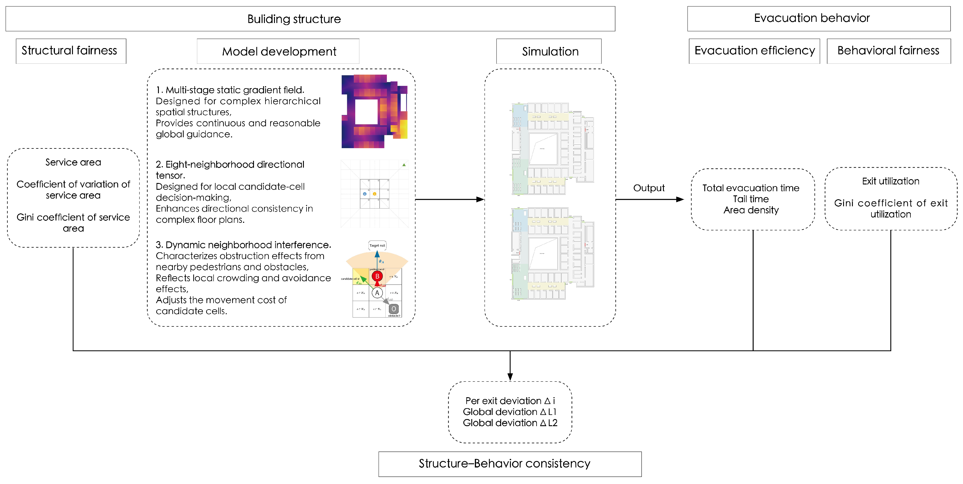
Figure 1. Research framework.
Sustainability 18 03286 g001
Figure 2. Decision-making logic.
Sustainability 18 03286 g002
Figure 3. Study case.
Sustainability 18 03286 g003
Figure 4. Exit locations in the two scenarios: (a) Scenario 1; (b) Scenario 2.
Sustainability 18 03286 g004
Figure 5. L-corridor field overlay.
Sustainability 18 03286 g005
Figure 6. Fundamental diagram fits: (a) density–speed; (b) density–flow.
Sustainability 18 03286 g006
Figure 7. Cumulative evacuation curves.
Sustainability 18 03286 g007
Figure 8. Boxplot of total evacuation time.
Sustainability 18 03286 g008
Figure 9. Time-normalized evacuation curves: (a) cumulative evacuation; (b) evacuation rate.
Sustainability 18 03286 g009
Figure 10. Boxplot of exit utilization U i .
Sustainability 18 03286 g010
Figure 11. Boxplot of behavioral Gini coefficient G U .
Sustainability 18 03286 g011
Figure 12. Boxplot of exit-level structure–behavior deviation Δ i .
Sustainability 18 03286 g012
Figure 13. Density time series in density measurement areas.
Sustainability 18 03286 g013
Figure 14. Density differences by scale: (a) real time scale; (b) normalized evacuation progress scale.
Sustainability 18 03286 g014
Table 1. Model parameters used in the simulations.
ParameterMeaningValue/Description
Δ x Grid size 0.4 m (spatial discretization)
Δ t Time step 0.333 s (derived from free walking speed)
v 0 Free walking speed 1.20 m s 1
α Static field weight 0.6 (fixed in advance, cross model validation)
β Pedestrian interference weight 0.1 (fixed in advance, cross model validation)
γ Obstacle interference weight 0.3 (fixed in advance, cross model validation)
kRepulsion strength scaling factor10 (dimensionless, used to match the magnitude with the non normalized S ( c ) )
δ Repulsion decay scale 0.1 m (empirical value, cross model validation)
r obs Equivalent obstacle radius 0.2 m (grid scale)
ω Directional weight value set 1 , 1 2 , 1 3 , 1 4 , 1 5 (rule setting)
Table 2. Cross-model validation of total evacuation time between the CA model and Pathfinder (Scenarios 1–5).
ScenarioCA Mean
(s)
Pathfinder Mean
(s)
Absolute Error
(s)
Relative Error
(%)
Shapiro–Wilk
p
Sign Test
p
Cohen’s
d
Equivalence
(5% Threshold)
120.9220.500.422.050.00000.00660.630PASS
222.5021.900.602.750.00040.00000.797PASS
322.3421.500.843.910.00000.00001.052PASS
423.5823.200.381.620.00020.01200.464PASS
523.0522.800.251.080.00000.00090.392PASS
Shapiro–Wilk test was used for normality testing. Sign test was used for directional consistency testing. Equivalence was assessed using a 5% relative error threshold.
Table 3. Fundamental diagram fitting parameters and goodness of fit for the Weidmann and Fruin models.
Model R 2 RMSEEffective Free-Flow Speed
v 0 eff (m/s)
Jam Density k j
(Person/m2)
Peak Flow
(Person/(m·s))
Critical Density
(Person/m2)
Weidmann0.9720.1282.411.092.140.93
Fruin0.9610.1522.140.93
v 0 eff denotes the effective free flow speed under discrete movement (including diagonal steps) using a displacement-based speed definition, and it is not a direct estimate of actual walking speed. This validation mainly focuses on the consistency of macroscopic characteristics such as R 2 /RMSE, critical density, and peak flow.
Table 4. Effect of exit location adjustment on total evacuation time.
MetricScenario 1 Mean (95% CI)Scenario 2 Mean (95% CI)Difference Mean (95% CI)Change (%)p-ValueHedges’ g
T total (s)23.31 (23.09, 23.55)18.65 (18.50, 18.81) 4.66 ( 4.95 , 4.39 ) 19.99 <0.0016.512
Table 5. Comparison of percentile evacuation times ( T 50 , T 90 , and T 95 ) between scenarios.
MetricScenario 1 Mean
(95% CI)
Scenario 2 Mean
(95% CI)
Difference Mean
(95% CI)
Change (%)p-ValueHedges’ g
T 95 (s)15.42 (15.34, 15.51)15.49 (15.40, 15.59)0.07 ( 0.05 , 0.20)0.460.259 0.225
T 90 (s)13.36 (13.28, 13.43)13.53 (13.45, 13.60)0.17 (0.06, 0.27)1.250.003 0.596
T 50 (s)5.81 (5.77, 5.86)6.03 (6.01, 6.05)0.213 (0.16, 0.27)3.67<0.001 1.572
Table 6. Comparison of tail evacuation phase indicators between scenarios.
MetricScenario 1 MeanScenario 2 MeanDifference MeanChange (%)Hedges’ g
T a i l 95 (s)7.893.16 4.73 59.95 5.909
T a i l R a t i o 95 (%)33.8016.90 16.90 50.00 5.703
T a i l 90 (s)9.955.12 4.83 48.54 6.275
T a i l R a t i o 90 (%)42.7027.40 15.30 35.90 6.096
T 95 T 90 (s)2.061.96 0.10 4.85 0.284
Table 7. Behavioral fairness comparison based on the Gini coefficient of exit utilization ( G U ).
MetricScenario 1 Mean (95% CI)Scenario 2 Mean (95% CI)Difference Mean (95% CI)Change (%)p-ValueHedges’ g
G U 0.356 (0.354, 0.357)0.320 (0.318, 0.321) 0.036 10.09 < 0.001 6.315
Table 8. Per-exit service area ( A i ) and service share in Scenario 1 and Scenario 2.
ExitScenario 1 Service Area (m2)Scenario 2 Service Area (m2)Scenario 1 Service Share (%)Scenario 2 Service Share (%)
Exit 166.40105.765.458.69
Exit 225.7661.602.115.06
Exit 3154.4097.6012.668.02
Exit 4146.08113.1211.989.29
Exit 590.8890.887.457.46
Exit 6153.44153.4412.5812.60
Exit 7149.12146.8812.2312.06
Exit 8133.76120.4810.979.90
Exit 912.6424.001.041.97
Exit 10286.88303.6823.5324.94
Table 9. Structural fairness metrics based on service area ( C V A and G A ) in Scenario 1 and Scenario 2.
MetricScenario 1Scenario 2
C V A 0.650.61
G A 0.330.29
Table 10. Global deviation metrics for structure–behavior consistency in Scenario 1 and Scenario 2.
MetricScenario 1 Mean (95% CI)Scenario 2 Mean (95% CI)Difference Mean (95% CI)Change (%)p-ValueHedges’ g
Δ L 1 0.267856 (0.267856, 0.267856)0.268208 (0.267849, 0.268709)0.000351 ( 0.000007 , 0.000853)0.1310.1408 0.297
Δ L 2 0.1079 (0.1074, 0.1084)0.1017 (0.1013, 0.1021) 0.0062 ( 0.0068 , 0.0055 ) 5.736 < 0.001 3.653
Δ m a x 0.062 (0.062, 0.063)0.056 (0.056, 0.056) 0.006 ( 0.007 , 0.005 ) 9.871 < 0.001 2.812
Scenario means and 95% CIs are rounded to three decimal places, difference values are reported with higher precision to avoid rounding to zero.
Table 11. Local peak density ( ρ max ) and high-density duration metrics by measurement area.
AreaMetricScenario 1 Mean
(95% CI)
Scenario 2 Mean
(95% CI)
Differencep-ValueHedges’ g
Area1 ρ max 0.600 (0.581, 0.619)0.593 (0.571, 0.614) 0.008 0.5990.105
Duration i 0.000 (0.000, 0.000)0.000 (0.000, 0.000)0.0000.000
Duration i r e f 0.000 (0.000, 0.000)0.000 (0.000, 0.000)0.0000.000
Area2 ρ max 1.208 (1.190, 1.225)1.203 (1.185, 1.220) 0.005 0.6930.079
Duration i 0.007 (0.000, 0.020)0.000 (0.000, 0.000) 0.007 0.3220.198
Duration i r e f 1.827 (1.589, 2.064)1.980 (1.729, 2.231)0.1530.378 0.176
Area3 ρ max 0.503 (0.498, 0.507)0.505 (0.498, 0.512)0.0030.563 0.115
Duration i 0.007 (0.000, 0.020)0.013 (0.000, 0.032)0.0070.563 0.115
Duration i r e f 0.000 (0.000, 0.000)0.000 (0.000, 0.000)0.0000.000
Area4 ρ max 1.536 (1.518, 1.555)1.541 (1.525, 1.557)0.0050.713 0.073
Duration i 0.013 (0.000, 0.040)0.000 (0.000, 0.000) 0.013 0.3220.198
Duration i r e f 4.207 (4.031, 4.382)4.067 (3.993, 4.141) 0.140 0.1460.292
Area5 ρ max 0.800 (0.797, 0.803)0.800 (0.797, 0.803)0.0001.0000.000
Duration i 0.000 (0.000, 0.000)0.000 (0.000, 0.000)0.0000.000
Duration i r e f 0.000 (0.000, 0.000)0.000 (0.000, 0.000)0.0000.000
For the Duration metrics, 95% confidence intervals are reported in parentheses. If the estimated lower bound is negative, it is truncated to 0. If a given metric equals 0 in both scenarios, the corresponding p-value is reported as “—”. Because some regional duration series contain a high proportion of zero values, the effect sizes for Duration i and Duration i r e f should be interpreted with caution.
Disclaimer/Publisher’s Note: The statements, opinions and data contained in all publications are solely those of the individual author(s) and contributor(s) and not of MDPI and/or the editor(s). MDPI and/or the editor(s) disclaim responsibility for any injury to people or property resulting from any ideas, methods, instructions or products referred to in the content.