Sustainability Analysis: Research on China’s Real Estate Economy and Business Based on the CFPS Data

Abstract

Housing prices exert a notable impact on labor force sustainability, a key component of socioeconomic sustainable development. Skyrocketing housing costs tend to postpone young adults’ marriage and childbearing schedules, reduce their fertility intentions, and eventually lead to a shrinking labor force. It is therefore essential to explore the intrinsic links between housing prices, fertility intentions, and labor force sustainability. Based on data on China’s commercial housing prices, fertility rates, and related socioeconomic indicators from 2005 to 2024, this paper analyzes the theoretical mechanisms of how housing prices affect fertility intentions. It examines the trends of housing prices, housing price-to-income ratios, and disposable income growth at the national level, and further discusses the heterogeneous characteristics of these indicators in eastern, central, western, and northeastern China. In addition, this study analyzes the overall trends and regional disparities of fertility rates, conducts regression analyses combined with mortality rates and population growth rates, and implements correlation analyses between housing prices and fertility rates at national and regional levels. Using 2018 and 2022 CFPS data with control variables including education years, household registration type, employment nature, gender, and number of siblings, an improved interaction terms fixed-effects model is adopted to empirically examine the impact of housing prices on fertility intentions. The reliability of the results is verified by three methods: parallel trend test, alternative estimation method, and data source replacement.

1. Introduction

As the core driving force for sustainable economic growth in society, the issue of population reproduction is not only a fundamental issue for the long-term development of a country, but also a strategic proposition that determines the rise and fall of a nation [1,2]. Currently, the global fertility rate shows a significant characteristic of “regional differentiation and overall decline”, with significant differences in fertility rates among countries with different levels of economic development and geographical locations, and is overall lower than historical levels [3,4]. Multiple factors, such as house prices, population mobility, the urbanization process, gender role cognition, changes in marriage and childbearing concepts, and labor market participation status, all have a crucial impact on fertility rate changes [5,6,7]. Population constitutes the bedrock of sustainable socioeconomic development [8,9]. In recent years, China’s fertility rate has shown a rapid decline trend, with increasingly prominent structural contradictions such as population aging and a shrinking labor supply, which have become key bottlenecks restricting the advancement of China-style modernization. Therefore, studying the impact of house prices on fertility rate and promoting sustainable labor force development is of great significance [10,11,12].

The theoretical research on fertility intentions not only determines the future population size and structure but also has a crucial impact on economic sustainable development through long-term changes in labor supply. Badolato et al. [13] drew on nationally representative data from the United States to investigate fertility rates through the dual lenses of life course and gender, offering novel insights into understanding the recent decline in fertility rates observed in the country. Zhong et al. [14] explored the effects of parental time investment and its gender disparities on Chinese residents’ fertility intentions, using empirical data from the 2020 wave of the China Family Panel Studies (CFPS). Miaci et al. [15] conducted research based on the birth sample survey data from the Italian National Institute of Statistics, indicating that mothers using formal childcare services are more likely to exhibit positive fertility behaviors. Sturm et al. [16] conducted an analysis based on samples of 18–45-year-old childless men and women from 12 European countries, finding that the positive correlation between partner relationship and fertility intentions gradually strengthened from the age of 18. Sligo et al. [17] evaluated the impact of fertility intentions at the age of 15 on fertility outcomes 30 years later, finding that fertility intentions during adolescence are shaped by social, political, and economic norms and may influence fertility decisions in adulthood. Grant et al. [18] drew on in-depth interview data gathered in rural Malawi in July 2019, in the aftermath of Cyclone Idai, and found that several factors influencing fertility rates arise from profound uncertainty about the future, alongside constraints imposed by a livelihood environment reliant on natural resources.

The exploration of the impact of house price levels on economic behaviors, such as society and families, serves as the prerequisite and foundation for conducting research on the correlation between house prices and fertility intentions. Hjalager et al. [19] conducted a study on the transaction patterns and regional price trends of second homes in Denmark from 1992 to 2020, revealing the investment and financialization logic behind it as well as potential conspicuous consumption behaviors. Dell’Anna et al. [20] conducted research on consumer behavior in the Singapore real estate market at different stages, finding that green labels could bring a significant premium to apartment prices. Ma et al. [21] investigated the implications of rural-urban migration for economic development, and their findings indicated that migrant households with a sense of social belonging saw a 4% increase in their monthly consumption expenditure. Hou et al. [22] analyzed indicators including the housing price-to-income ratio and housing price-to-rent ratio using Beijing’s housing price data spanning 2014 to 2024, and identified clear signs of a significant price bubble in the real estate market during 2016 and 2017. Hu et al. [23] conducted research based on a comprehensive database of corporate relocation events in the United States, finding that relocation enterprises with larger staff sizes and stronger economic foundations had a more significant positive spillover effect on house price growth. House price fluctuations typically affect urban development, enterprise operations, and the financial credit system, thereby having a profound impact on the overall economy [24,25,26].

Exploring the correlation between house prices levels and residents’ fertility intentions is a key research direction that influences the economic trend of a country. Van Wijk et al. [27] discovered through research on the correlation between house prices and fertility rates in the Netherlands that there is a correlation between rising house prices and declining fertility rates, and the decline in fertility rates among the renting population is more significant. Ang et al. [28] used a regression discontinuity design, taking China’s housing market policies in 2006 as the research entry point, to explore the impact of housing wealth on fertility outcomes, and found that for every 1% increase in housing wealth, the fertility rate increased by 0.18%. Jin et al. [29] conducted an empirical study using questionnaire survey data on housing inclusiveness and fertility intentions across 35 Chinese cities, and their results revealed that housing cost burdens exert a significantly positive effect on residents’ perceived demand for social housing. Blaszke et al. [30] analyzed pertinent data from cities in Northwestern Poland, finding a marked positive correlation between urban rankings and housing prices in 2020. In general, housing prices exert an influence on fertility rates primarily through multiple channels, including economic squeeze, delayed marriage and childbearing, constraints on living space, shifts in psychological and social expectations, and disparities in wealth effects [31,32,33,34].

This paper is based on the house prices and fertility rate data of China from 2005 to 2024. It conducts an analysis through correlation analysis and an improved interaction terms fixed effects model. The outline of the paper is as follows: First, it studies the theoretical basis and mechanism of the impact of house prices on fertility intentions. Second, it examines the changing patterns of overall house prices, sales area, and the area of state-owned land transfer in China. The study is conducted regionally, including the eastern, central, western, and northeastern regions, analyzing the income–price ratio, the correlation between house prices and disposable income growth rate, and the correlation between house prices and disposable income. We also conduct an independent analysis of the housing price fluctuation rate. Third, this study explores the evolutionary patterns of China’s national and regional fertility rates and puts forward an analytical framework for fertility rates and fertility intentions. Fourth, it conducts correlation modeling for house prices and fertility rates at the overall and regional levels, and studies the correlation patterns between the two. Fifth, it uses a regression model based on the improved interaction terms fixed effects model to model and analyze the impact of house prices on fertility intentions and conducts robustness tests using three methods. Finally, the detailed conclusions are outlined.

2. Theoretical Mechanism Analysis of the Impact of House Prices on Fertility Rate

Fertility intentions are shaped by a diverse array of factors, including the political context, cultural traditions, economic costs, social policies, family structure, individual traits, and cognitive perceptions. This chapter focuses on the research on the impact of house prices on fertility intentions, drawing on the classic dual fixed-effects model [35] and improving it to examine the theoretical mechanism of the effect of house prices on residents’ fertility intentions. The maximization of family effects is as follows:

Then the expression for maximizing household utility is:

$$Max{L}_{i,E_h,E_w}=L(i,E_h,E_w)$$

(1)

$$\mathrm{s}.\mathrm{t}.\hspace{1em}{r}^{e}i+r^h(c+k{i}^{\beta })=T+{\displaystyle \sum _{j=h,i}{Z}_j(1-E_j)}$$

(2)

where $i$ is the number of children, $h$ is husband, $w$ is wife, $E_h$ and $E_w$ are the income of the husband and the wife, $r^e$ and $r^h$ are the costs of having children and house purchase price, $c$ is the initial housing area, $k$ and $k{i}^{\beta }$ are the housing area of a family with one child or multiple children, $T$ is the initial family wealth, and $(1-E_j)$ is the time spent by the husband and the wife on labor work.

The optimization conditions of the Lagrangian function are as follows:

$$L_1-\mu (r^e+r^{h}k{i}^{\beta -1})=0$$

(3)

$$L_2-\mu Z_h=0$$

(4)

$$L_3-\mu Z_w=0$$

(5)

where $\mu$ is Lagrange multiplier. The Lagrange multiplier method is suitable for solving constrained optimization problems [36]. Formula (3) can be used to calculate Formula (6) as follows:

$$L_1/\mu =r^e+r^{h}k{i}^{\beta -1}$$

(6)

where $L_1/\mu$ is the fertility shadow price, and $r^e+r^{h}k{i}^{\beta -1}$ is house prices.

To more intuitively capture the effect of housing prices on the fertility rate, we derive the comparative static relationship between fertility intentions and housing prices by computing the partial derivatives of Formulas (3)–(5) with respect to housing prices, as follows:

$$\left[\begin{array}{cccc}0& -r^e-r^{h}k{i}^{\beta -1}& -Z_h& -Z_w\\ -r^e-r^{h}k{i}^{\beta -1}& Z_{11}-\mu r^{h}k\beta (\beta -1)i^{\beta -2}& L_{12}& L_{13}\\ -Z_h& L_{21}& L_{22}& L_{23}\\ -Z_w& L_{31}& L_{32}& L_{33}\end{array}\right]\left[\begin{array}{c}𝜕\mu /𝜕r^h\\ 𝜕i/𝜕r^h\\ 𝜕E_h/𝜕r^h\\ 𝜕E_w/𝜕r^h\end{array}\right]=\left[\begin{array}{c}H\\ \mu r^{h}k\beta i^{\beta -1}\\ 0\\ 0\end{array}\right]$$

(7)

Then the expression for maximizing household utility simplifies to $B$. The determinant of the first term on the left side of Formula (7) is $\left|B\right|$. The expression of $B$ without the first row and first column is the effect of house prices on fertility intentions, as follows:

$${\displaystyle \frac{𝜕i}{𝜕r^h}}=-H{\displaystyle \frac{\left|B_{12}\right|}{\left|B\right|}}+\mu k\beta i^{\beta -1}{\displaystyle \frac{\left|B_{22}\right|}{\left|B\right|}}=-H{\displaystyle \frac{𝜕n}{𝜕T}}+\mu k\beta i^{\beta -1}{\displaystyle \frac{\left|B_{22}\right|}{\left|B\right|}}<0$$

(8)

where ${\displaystyle \frac{𝜕n}{𝜕T}}>0$ and $\left|B\right|<0$.

$$\left|B_{22}\right|=\left[\begin{array}{ccc}0& -Z_h& -Z_w\\ -Z_h& L_{22}& L_{23}\\ -Z_w& L_{32}& L_{33}\end{array}\right]>0$$

(9)

where ${\displaystyle \frac{𝜕n}{𝜕T}}$ is the income effect of reproductive demand, $\left|B_{22}\right|$ is a 3rd-order matrix representing the effectiveness function for the case where the number of family children is zero.

Equation (8) captures the effect of housing price changes on fertility intentions when housing consumption serves as a derived demand for fertility. It shows the changes in household budget constraints and the consumption of housing substitutes caused by house price fluctuations, as well as the influence of these on fertility intentions, namely the income effect and substitution effect of house prices on fertility intentions. $-H{\displaystyle \frac{\left|B_{12}\right|}{\left|B\right|}}$ indicates that an increase in house prices will lead to a tightening of household budget constraints, thereby exerting a negative income effect with a weight of housing area $H$ on fertility intentions. $\mu k\beta i^{\beta -1}{\displaystyle \frac{\left|B_{22}\right|}{\left|B\right|}}$ represents the shadow price of having children, and the scale effect is determined by the number of children (one or more). Therefore, it can be seen that an increase in house prices will lead to a decrease in residents’ fertility intentions.

The comparative static analysis of the household utility maximization model yields the core conclusion that housing price hikes exert a negative inhibitory effect on residents’ fertility intentions ($𝜕i/𝜕r^h<0$), which is essentially driven by two key mechanisms: the rise in fertility shadow price caused by housing price increases and the tightened household budget constraints weighted by actual housing area H. Notably, this negative effect is not homogeneous across all groups, but is amplified among households with greater housing purchase cost pressure and stronger actual fertility demand—this heterogeneous theoretical implication constitutes the fundamental design basis for the subsequent empirical analysis framework. To empirically test the above theoretical mechanism, the core theoretical parameters and heterogeneous characteristics need to be translated into measurable empirical indicators: the housing price rh and housing area H (the core parameters reflecting housing cost pressure) are operationalized as the city-level house price-to-income ratio in the empirical study; the heterogeneous fertility demand (the key premise for the theoretical conclusion to hold) is identified by the age grouping of reproductive willingness and capacity. The improved interaction terms fixed effects model with the interaction term of housing cost pressure and reproductive age group is thus constructed, which directly targets the core research object of the theoretical model and realizes the rigorous empirical test of the theoretical mechanism.

3. Regularity Analysis of China’s House Prices

3.1. Analysis of the Overall Characteristics of House Prices

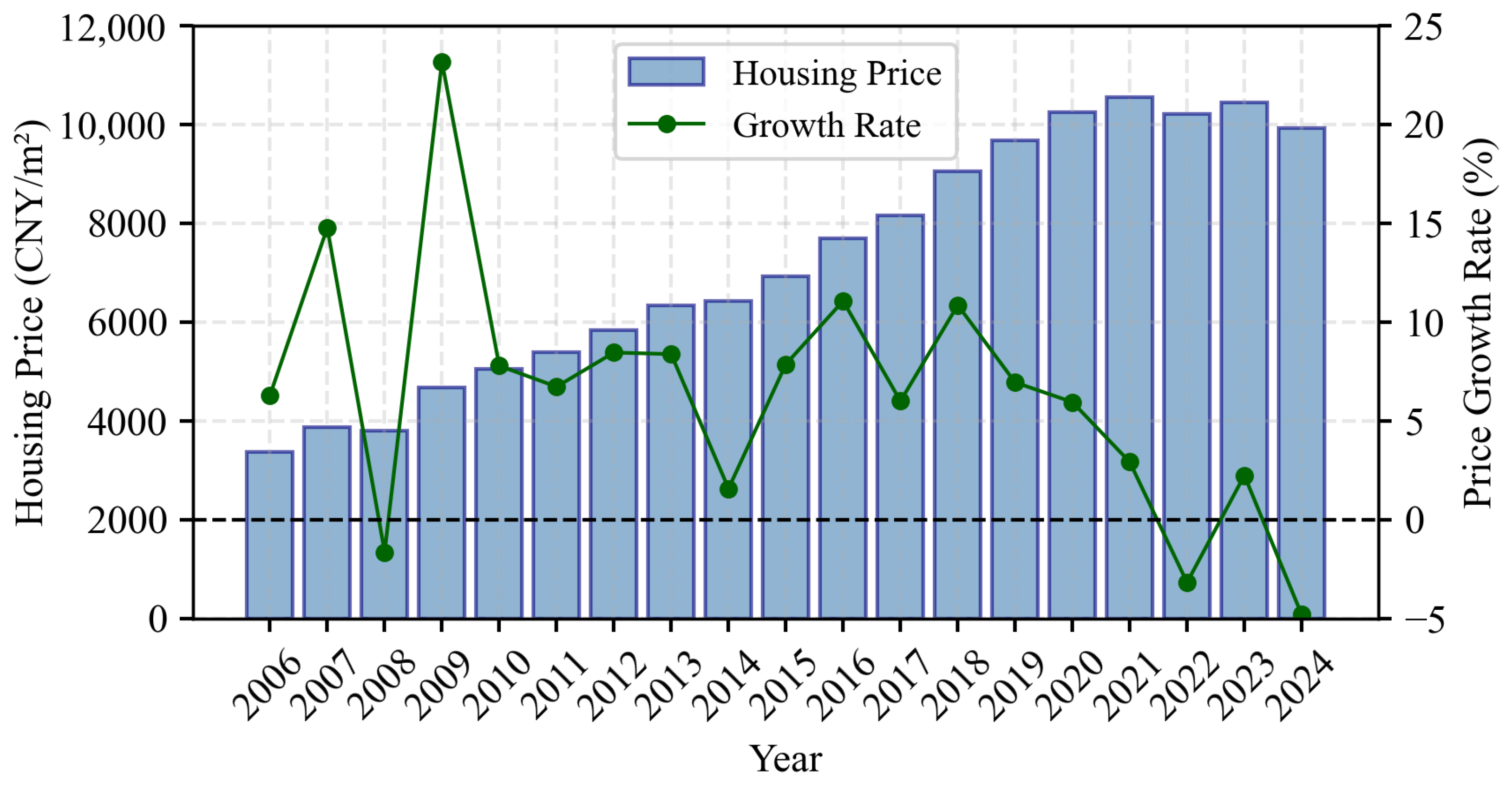
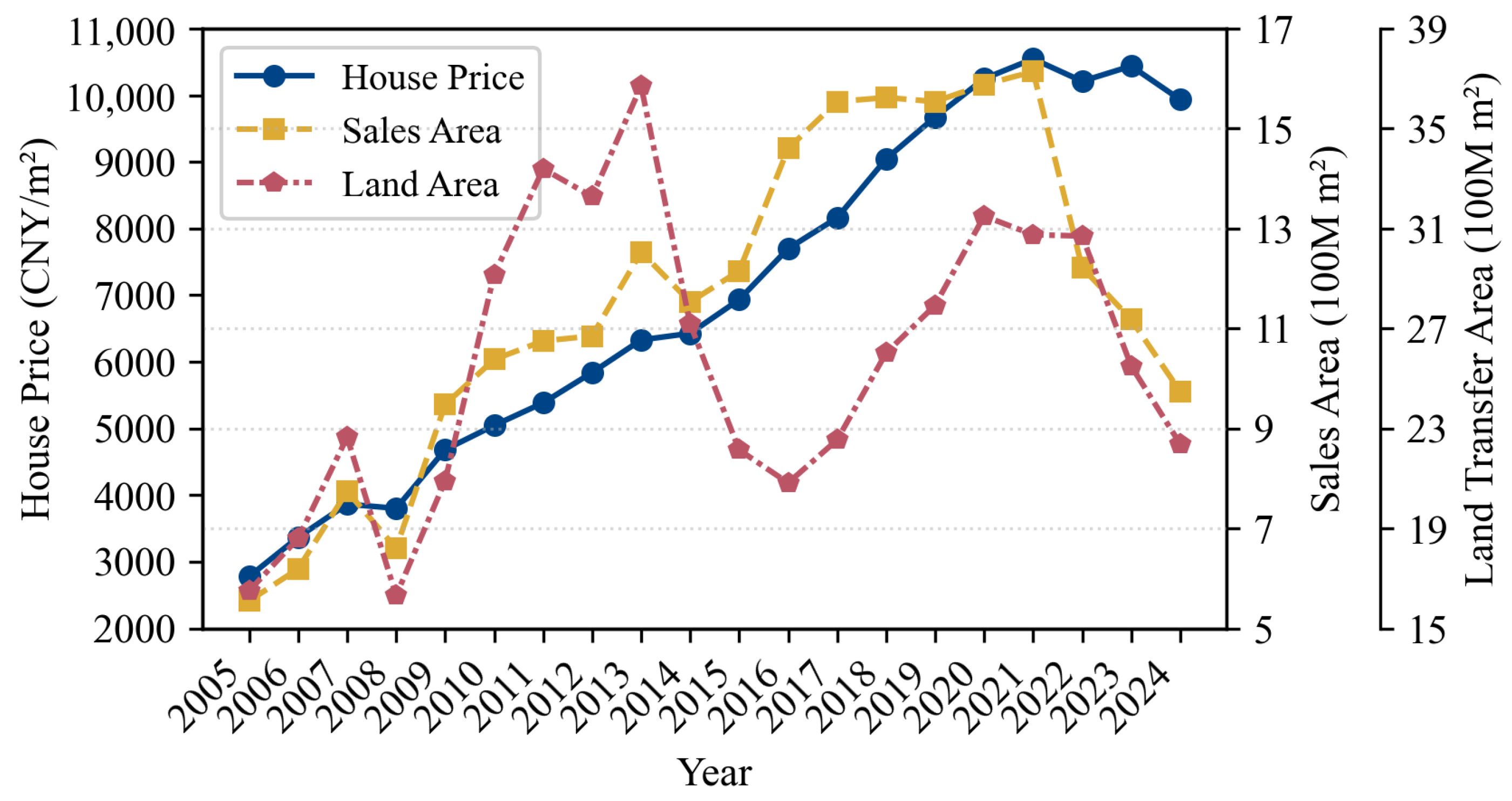
Figure 1 illustrates the trends of China’s commercial housing prices and their corresponding growth rates. It is evident that the indicators maintained an overall upward trajectory from 2006 to 2021, before shifting to a downward pattern between 2021 and 2024. The commercial house prices in China increased from 3168 $\mathrm{CNY}/{\mathrm{m}}^2$ in 2006 to 9935 ${\mathrm{CNY}/\mathrm{m}}^2$ in 2024, with an increase rate of 213.60%. In 2006, the per capita housing area in urban areas of China was less than 27 ${\mathrm{m}}^2$, and residents’ requirements for housing quality were not high. The core attribute of housing was consumption. From 2006 to 2029, the growth rate of house prices was relatively high, which was related to the 29th Summer Olympic Games held in China in 2008. In addition, in 2006, the state officially established the real estate industry as a pillar industry of the national economy, which laid the institutional foundation for the golden development stage of the real estate industry. Multiple factors, such as policy inclination and the free flow of population elements, jointly contributed to the significant fluctuations in the growth rate of commercial house prices in 2008. The growth rate of house prices showed a downward trend after 2018, and house prices also showed a downward trend after 2021.

The housing price data in this study adopts the official nominal price caliber of China’s real estate market. Although nominal prices do not exclude the impact of inflation, the continuous decline of the income-to-house-price ratio (Section 3.1) directly reflects the actual decline of residents’ housing affordability; meanwhile, the consistent nominal price caliber ensures the comparability of cross-regional and time-series data, and does not affect the reliability of the relative change trend of housing prices and the correlation conclusion between housing prices and fertility rates.

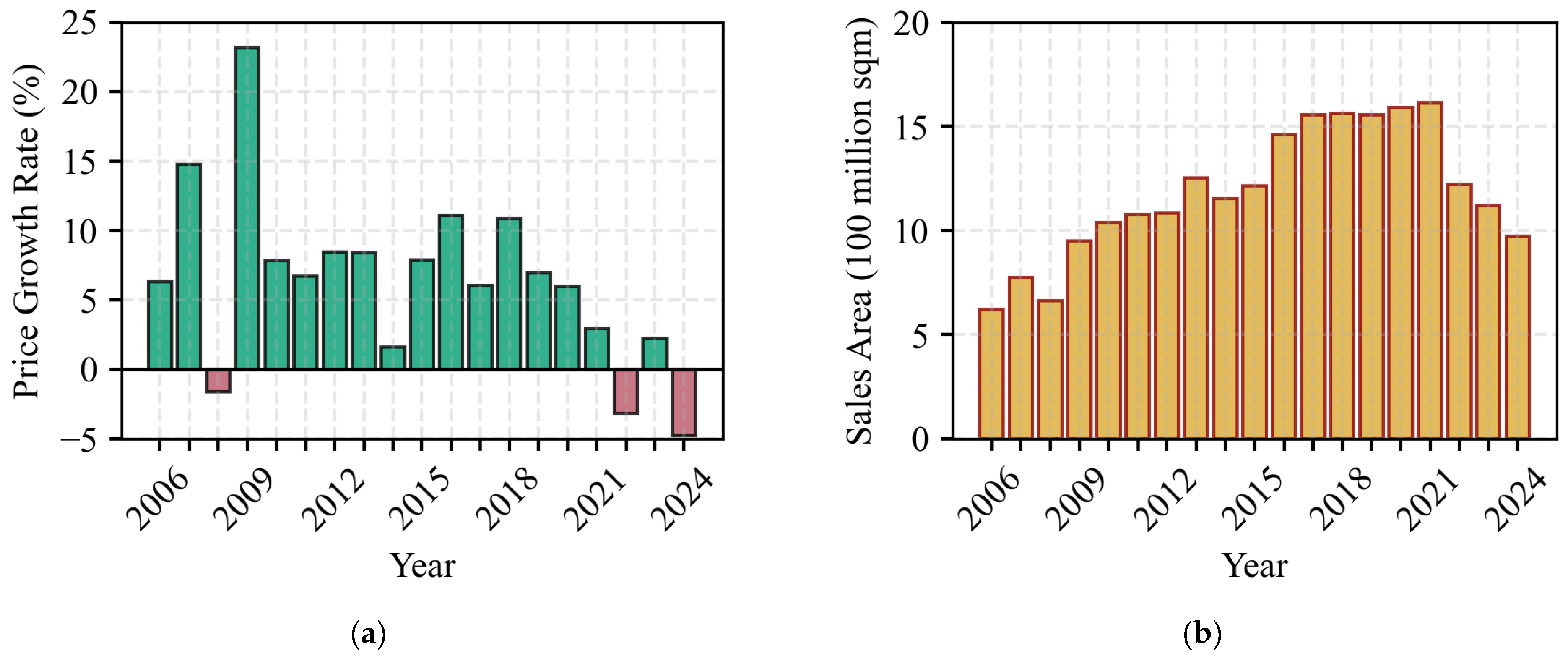
Figure 2a is a bar chart showing the growth rate of house prices. It can be clearly seen that there were three negative growths in the house price growth rate in 2008, 2022, and 2004. The main reason for the negative growth in the house price growth rate in 2008 was the 2008 financial crisis. To regulate the real estate market, the government rolled out targeted policies to stimulate home purchases, which led housing prices to resume positive growth after 2009. The house prices showed a significant downward trend in 2022 and 2024, which was related to the housing shortage and shrinking demand. The government issued the first purchase restriction order in 2010, successfully limiting the excessive growth of house prices. However, due to the increase in residents’ rigid housing demand, house prices showed an upward trend from 2011 to 2021. Figure 2b shows the available sales area of houses. It can be seen that it was also affected by the 2008 financial crisis. The available sales area decreased for the first time in 2008. By comparing Figure 1 and Figure 2b, it can be observed that both house prices and available sales area have shown a downward trend after 2021.

Table 1. China’s commercial house prices, house prices growth rates, and available housing sales areas. Source: National Bureau of Statistics of China (https://data.stats.gov.cn; accessed on 2 November 2025), 2005–2024.

Year	House Prices (CNY/m2)	Growth Rate (%)	Sales Area (100 Million m2)	Year	House Prices (CNY/m2)	Growth Rate (%)	Sales Area (100 Million m2)
2005	3168	14.04	5.55	2015	6932	7.86	12.15
2006	3367	6.29	6.19	2016	7699	11.06	14.6
2007	3864	14.77	7.74	2017	8160	5.99	15.54
2008	3800	−1.65	6.6	2018	9045	10.85	15.62
2009	4681	23.18	9.48	2019	9673	6.94	15.54
2010	5045	7.78	10.38	2020	10,248	5.94	15.88
2011	5384	6.72	10.75	2021	10,546	2.91	16.14
2012	5839	8.45	10.85	2022	10,210	−3.19	12.22
2013	6328	8.37	12.53	2023	10,438	2.23	11.18
2014	6427	1.56	11.53	2024	9935	−4.82	9.74

presents the statistical data on China’s commercial housing prices, housing price growth rates, and available housing sales areas, which correspond to Figure 1 and Figure 2. As can be seen from Table 1, the house prices dropped by 64 ${\mathrm{CNY}/\mathrm{m}}^2$ for the first time in 2008, with a growth rate of −1.65%. In 2009, due to the introduction of the national estimated home purchase policy, the growth rate reached its maximum value of 23.18%. The second and third declines in the growth rate corresponded to −3.19% in 2022 and −4.82% in 2024, respectively.

Figure 3 illustrates housing prices, sales area, and the area of allocated state-owned land. The correlation coefficient between housing prices and sales area is 0.753, indicating a strong positive correlation. This suggests that housing prices and sales volume tend to move in the same direction, which reflects a demand-driven price increase during the market expansion period. The correlation coefficient between house prices and allocation area is 0.326 (a weak positive correlation), which indicates that the direct impact of land supply on house prices is limited. This suggests that house prices are mainly driven by demand-side factors (monetary policy, credit conditions, and population structure). The correlation coefficient between sales area and allocation area is 0.443 (a moderate positive correlation), which indicates a certain correlation, but not strong enough. Land supply provides potential supply, but actual development depends on market conditions.

3.2. Analysis of the Regional Characteristics of House Prices

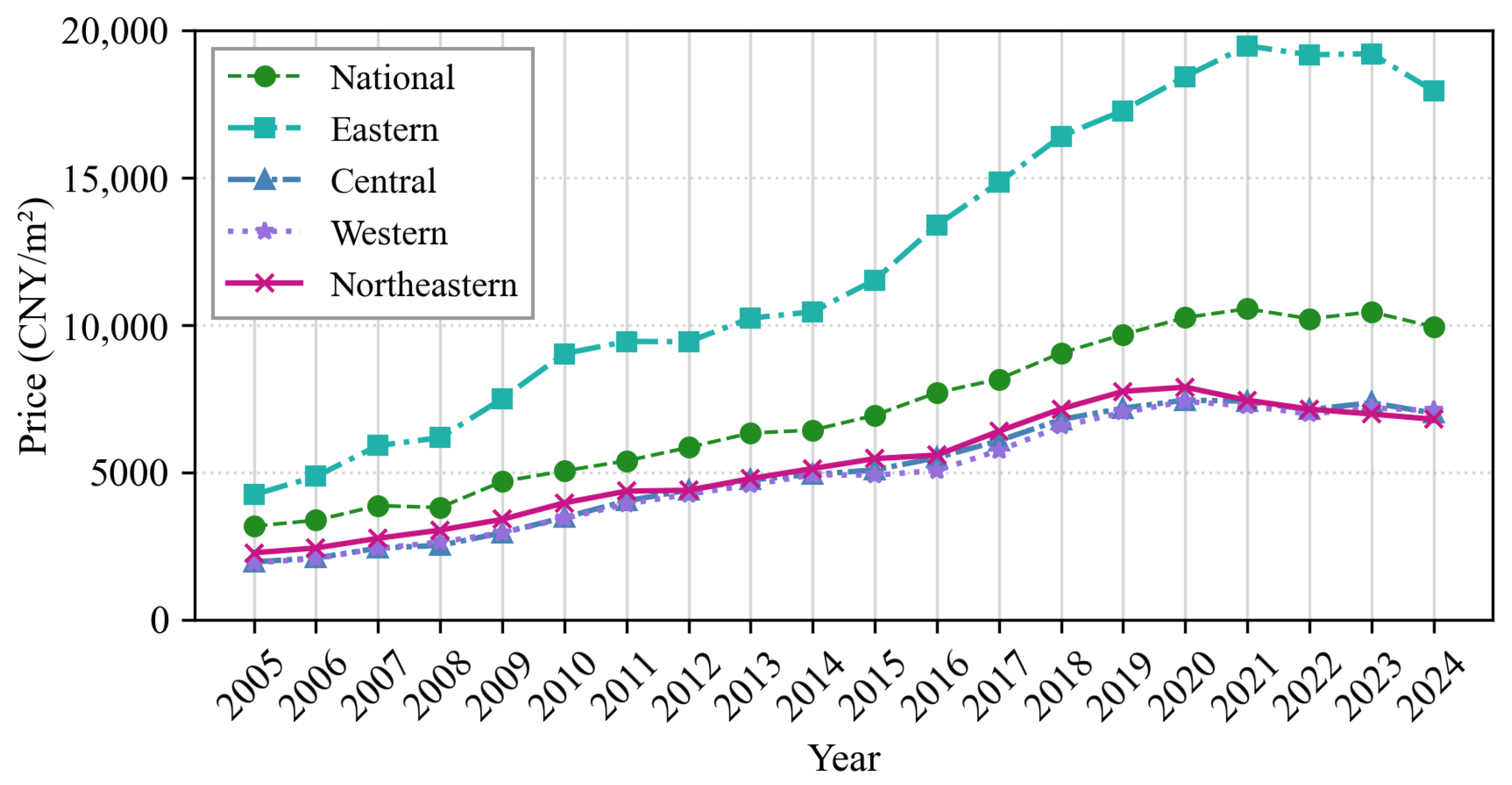
The differences in house prices across regions in China are driven by multiple factors such as economic development levels, population, industries, policies, and resources. Figure 4 shows the statistics of house prices in various regions of China. It can be observed that from 2005 to 2021, the house prices in the entire country, the eastern region, the central region, the western region, and the northeastern region all showed an upward trend. From 2021 to 2024, they showed a downward trend. The house prices in the central, western, and northeastern regions are similar, while the house prices in the eastern region are the highest. Elevated housing prices in eastern China are primarily driven by robust economic fundamentals, dense population concentration, superior public resources, and scarce land supply. Coupled with advanced industrial structures, mature financial systems, favorable policy support, and strong market expectations, these factors form a self-reinforcing cycle characterized by robust housing demand, constrained supply, and high land premiums. Key eastern economic zones, including the Yangtze River Delta, Pearl River Delta, and the Beijing-Tianjin-Hebei region, account for nearly 60% of China’s total GDP, with their per capita GDP and per capita disposable income outperforming the central and western regions by 30% to 80% on average.

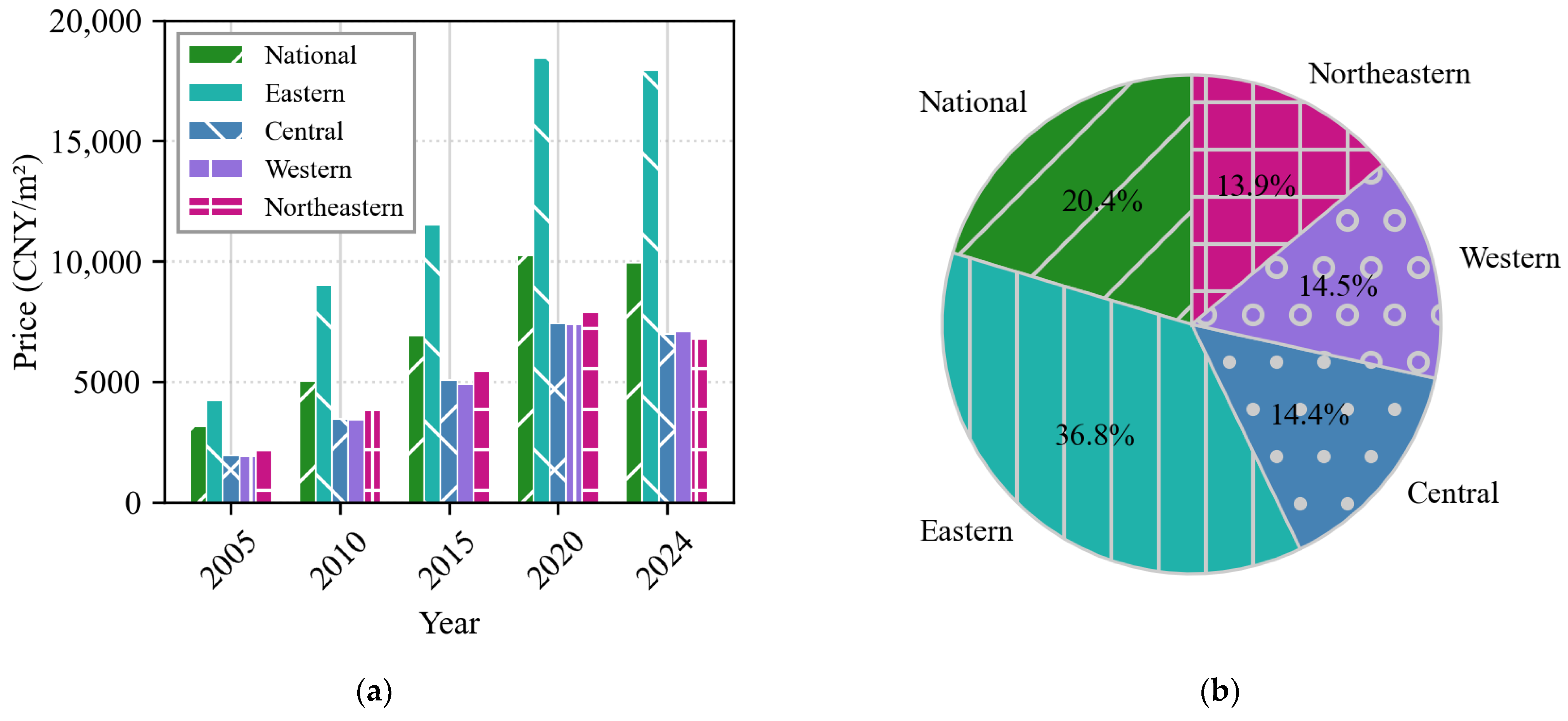
Figure 5a displays a bar chart that illustrates housing prices in 2010, 2012, 2020, 2024, and 2025. This graphical representation facilitates an intuitive and clear comparison of housing prices across different regions over the examined years. Correspondingly,

Table 2. China’s regional house prices in 2025, 2010, 2012, 2020, 2024 statistics. Source: National Bureau of Statistics of China (https://data.stats.gov.cn; accessed on 2 November 2025), 2005–2024.

Year	Nationwide (CNY/m2)	Eastern (CNY/m2)	Central (CNY/m2)	Western (CNY/m2)	Northeast (CNY/m2)
2005	3167.66	4233.24	1952.30	1923.35	2261.63
2010	5045.00	9022.60	3461.17	3425.83	3957.00
2015	6932.00	11,525.30	5077.17	4897.58	5459.33
2020	10248.00	18,433.50	7444.83	7403.08	7886.00
2024	9935.00	17,945.70	7001.83	7089.00	6796.00

presents the detailed housing price statistics for China’s regions, which are compiled based on the data shown in Figure 5a. From Figure 5a and Table 2, it can be seen that in 2024, the house price in the eastern region (17,945.70 ${\mathrm{CNY}/\mathrm{m}}^2$) was 4.24 times that of 2005 (4233.24 ${\mathrm{CNY}/\mathrm{m}}^2$), and it decreased by 7.8% compared to the peak in 2020. In the central region, the house price in 2024 (7001.83 ${\mathrm{CNY}/\mathrm{m}}^2$) was 3.59 times that of 2005 (1952.30 ${\mathrm{CNY}/\mathrm{m}}^2$), and it decreased by 5.9% compared to the peak in 2020. In the western region, the house price in 2024 (7089.00 ${\mathrm{CNY}/\mathrm{m}}^2$) was 3.69 times that of 2005 (1923.35 ${\mathrm{CNY}/\mathrm{m}}^2$), and it decreased by 4.3% compared to the peak in 2020. In the northeastern region, the house price in 2024 (6796.00 ${\mathrm{CNY}/\mathrm{m}}^2$) was 3.00 times that of 2005 (2261.63 ${\mathrm{CNY}/\mathrm{m}}^2$), and it decreased by 13.8% compared to the peak in 2020, with the largest decline in the northeastern region. Figure 5b is a pie chart comparing regional house prices in 2024 with those in Figure 5a. It is clearly shown that the eastern region’s house price was 80.6% higher than the national average. The house prices in the central, western, and northeastern regions were all lower than the national average, being 29.5%, 28.7%, and 31.6% lower, respectively.

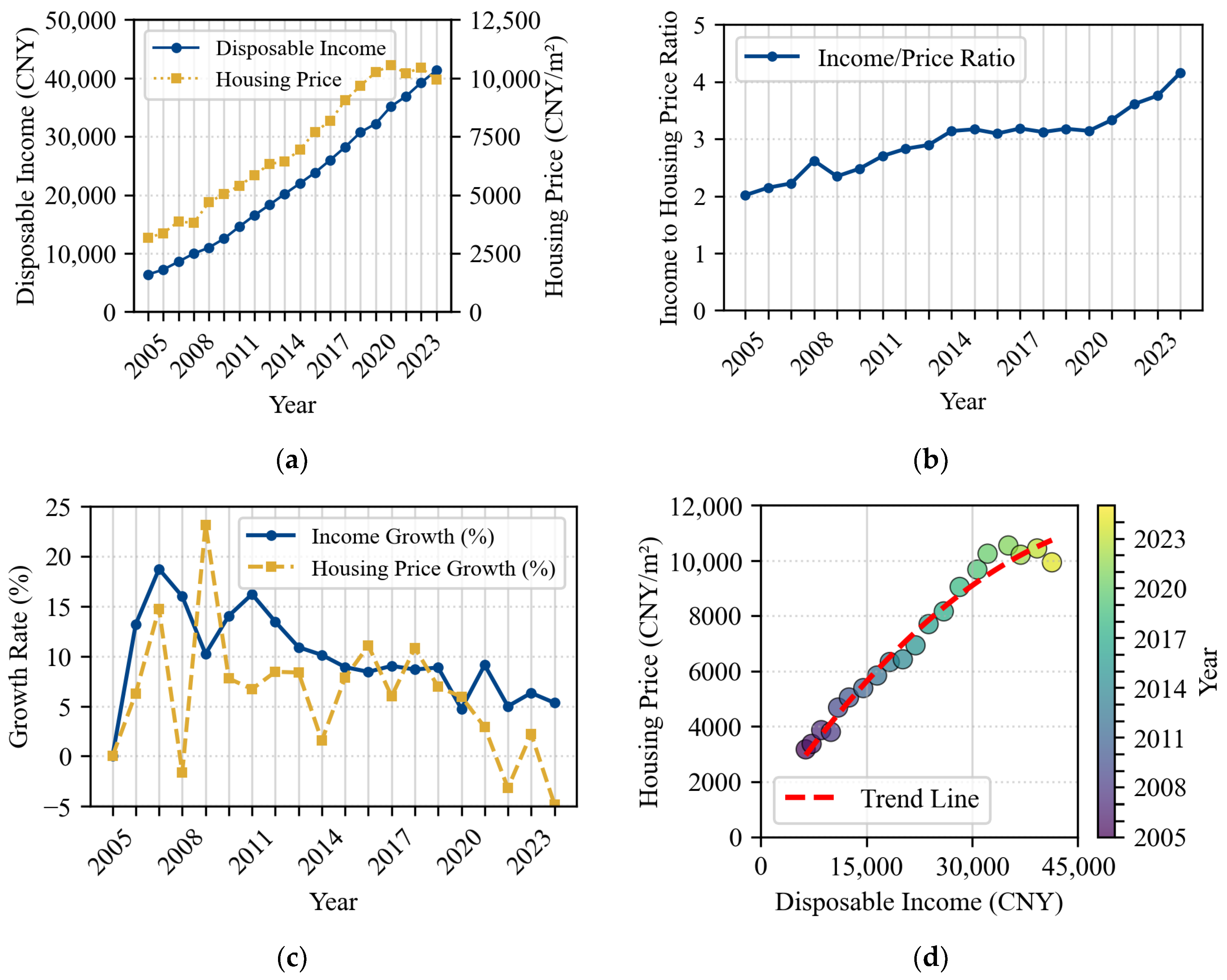
Figure 6a shows the relationship between house prices and disposable income. It can be seen that the income has increased from 10,493 ${\mathrm{CNY}/\mathrm{m}}^2$ in 2005 to 39,218 ${\mathrm{CNY}/\mathrm{m}}^2$ in 2024, a growth of 273.7%. The house prices have risen from 3167 ${\mathrm{CNY}/\mathrm{m}}^2$ in 2005 to 10,509 ${\mathrm{CNY}/\mathrm{m}}^2$ in 2024, representing a growth of 231.8%. Both income and house prices show a continuous upward trend, reflecting China’s economic development and urbanization process. The two curves grow basically in sync, demonstrating the positive correlation between house prices and economic development levels. Figure 6b shows the income-to-house-price ratio. The income-to-housing-price ratio is defined as the quotient of annual per capita disposable income divided by housing price per square meter. A continuous decline in this ratio reflects that the housing affordability pressure on Chinese residents has been intensifying over time. In line with international norms, a reasonable interval for the income-to-housing-price ratio ranges from 5 to 10, yet the level in China is considerably lower than this international benchmark. Figure 6c shows the income growth rate. It can be seen that the average annual growth rate is approximately 7.5%. From 2020 to 2024, the growth rate further slowed down to 4–6%. The house price growth rate fluctuates greatly and is significantly affected by policies. The income growth rate is relatively stable and has a stronger correlation with the economic fundamentals. Figure 6d is the correlation analysis between house prices and disposable income. It can be seen that income and house prices show a clear positive correlation. As income increases, house prices rise accordingly.

3.3. Analysis of the Rate of Change in House Prices

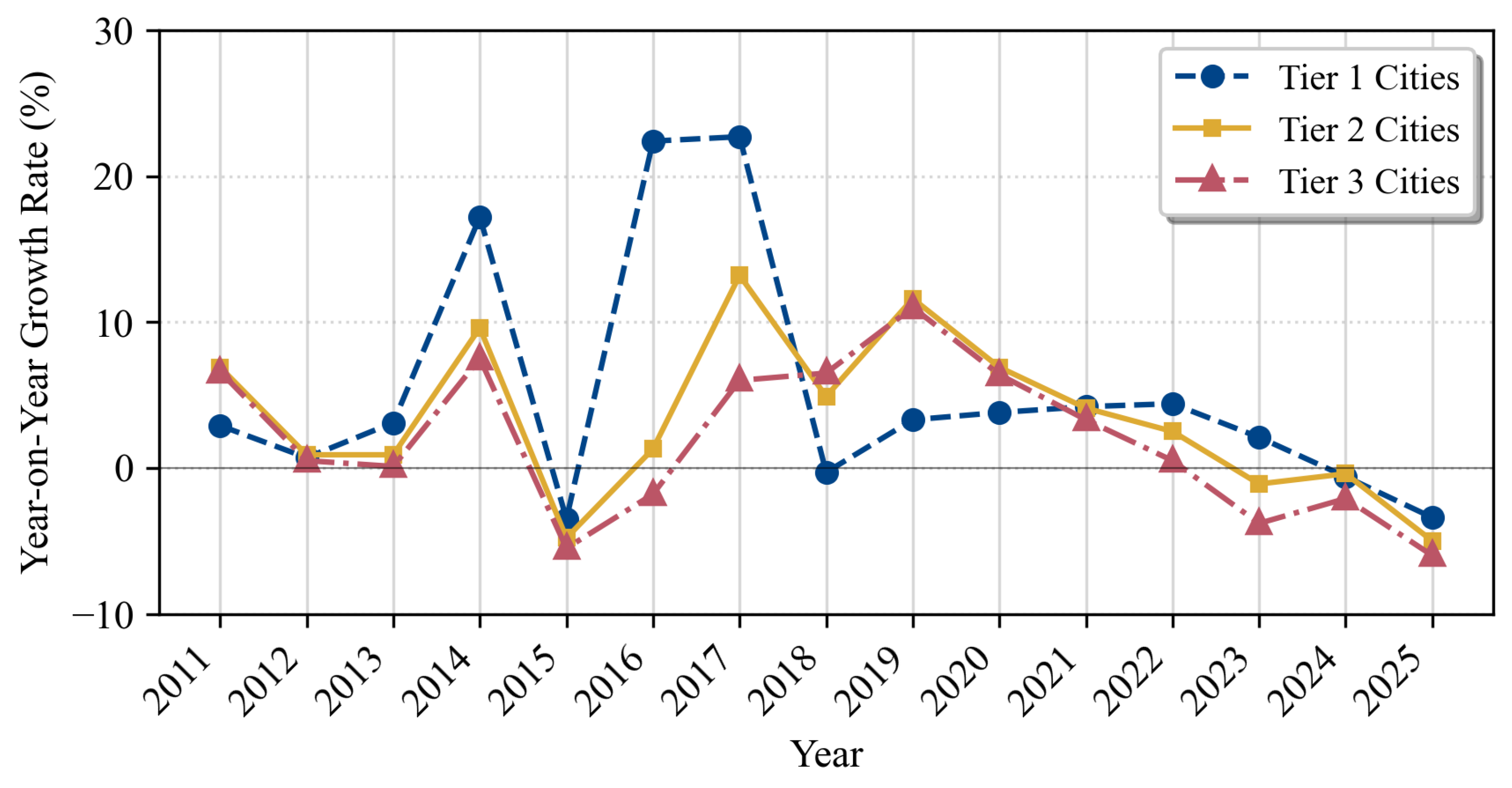
Figure 7 depicts the variations in residential price indices across first-tier, second-tier, and third-tier cities. China has four first-tier cities, namely Beijing, Shanghai, Guangzhou, and Shenzhen. The house prices in these first-tier cities have always maintained a high growth trend. Over the past 15 years, the average growth rate has reached 5.27%, and the fluctuation range has also been the most significant. In 2017, the growth rate peaked at 22.7%, while in 2015, it dropped to −3.5%, with a difference of 26.2%. As the indicator of the real estate market, the market changes in first-tier cities usually precede those in other cities at different levels.

There are 31 second-tier cities in China, including Tianjin, Shijiazhuang, Taiyuan, Hohhot, Shenyang, Dalian, Changchun, Harbin, Nanjing, Hangzhou, Ningbo, Hefei, Fuzhou, Xiamen, Nanchang, Jinan, Qingdao, Zhengzhou, Wuhan, Changsha, Nanning, Haikou, Chongqing, Chengdu, Guiyang, Kunming, Xi’an, Lanzhou, Xining, Yinchuan, and Urumqi. The house price trends in these second-tier cities are relatively stable. The average growth rate over the past 15 years was 3.43%, which is between that of the first-tier and third-tier cities. Market dynamics in these second-tier cities display a certain lag relative to first-tier cities, yet their reaction to market fluctuations remains relatively pronounced. During the market adjustment period of 2025, housing prices in these second-tier cities declined by 5.0%, which reflects their weaker capacity to resist market risks.

There are 35 third-tier cities in China, including Tangshan, Qinhuangdao, Baotou, Dandong, Jinzhou, Jilin, Mudanjiang, Wuxi, Xuzhou, Yangzhou, Wenzhou, Jinhua, Bengbu, Anqing, Quanzhou, Jiujiang, Ganzhou, Yantai, Jining, Luoyang, Pingdingshan, Yichang, Xiangyang, Yueyang, Changde, Shaoguan, Zhanjiang, Urumqi, Zhanjiang, Guilin, Beihai, Sanya, Luzhou, Nanchong, Zunyi, and Dali. The growth rate of house prices in these third-tier cities is at the lowest level among all levels of cities. The average growth rate over the past 15 years is only 1.95%, with a relatively smooth fluctuation range. Market operations demonstrate greater stability, accompanied by a pronounced lag effect: the growth peak of this market cycle only emerged in 2019, two years later than that of first-tier cities.

4. Regularity Analysis of China’s Fertility Rate

4.1. Analysis of the Overall Characteristics of Fertility Rate

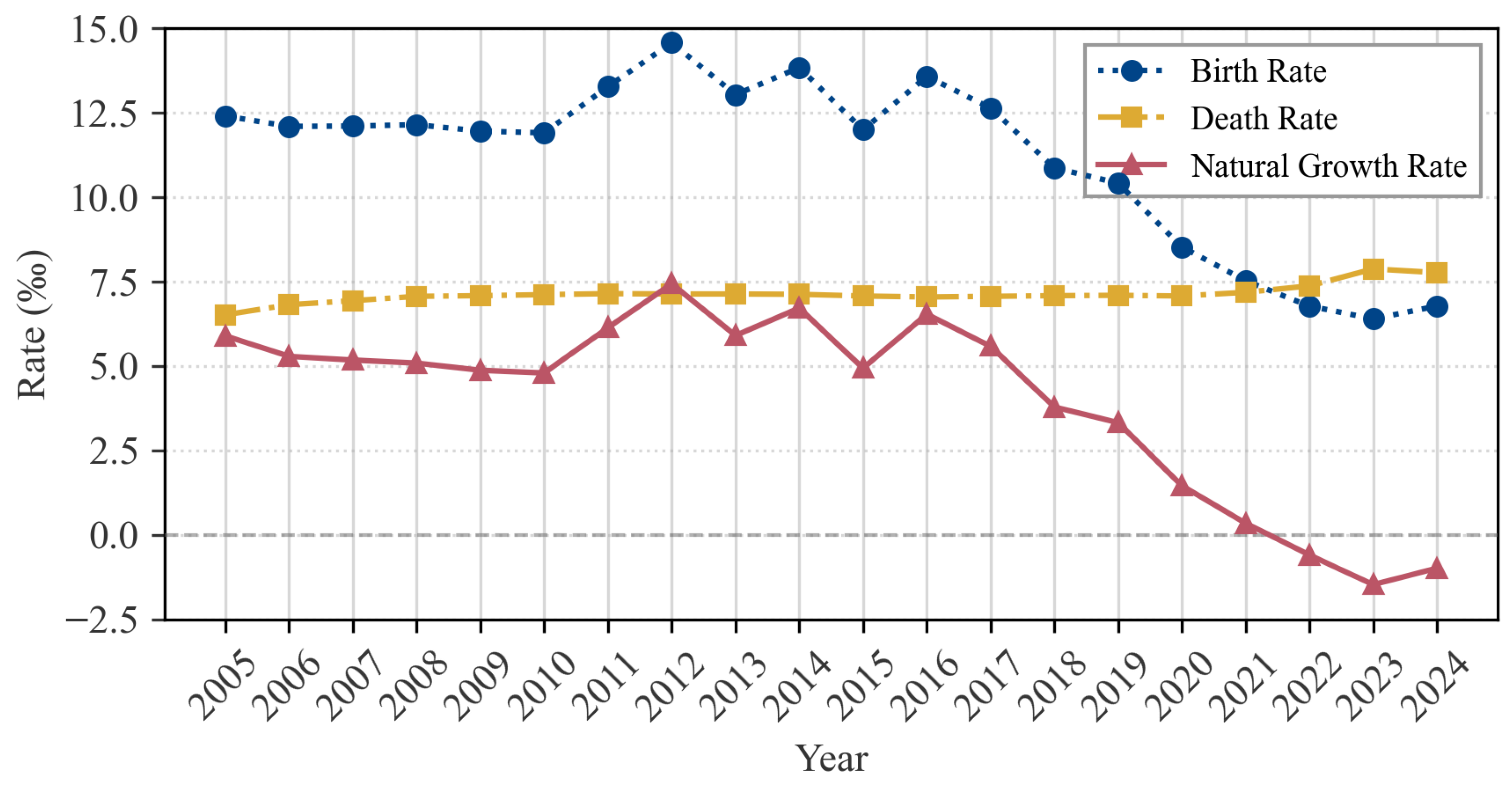
Figure 8 illustrates the trends of the crude birth rate, crude death rate, and natural population growth rate. It is evident that the natural growth rate presents a continuous downward trend, falling by 45.4% from 12.4‰ in 2005 to 6.77‰ in 2024. Moreover, the birth rate has been affected by two major policy shocks. The first policy shock took place after the implementation of the two-child policy in 2016, which lifted the birth rate from 11.99‰ in 2015 to 13.57‰ in 2016. The second policy shock occurred after the three-child policy in 2021, reducing the birth rate to 7.52%, indicating that the policy effect was not significant. Additionally, it can be seen that the birth rate of 6.77% in 2022 was the first to fall below the international low fertility warning line (7%), and it slightly rebounded in 2023 and then dropped again to 6.77% in 2024. The death rate shows a slow upward trend, rising from 6.51% in 2005 to 7.76% in 2024, mainly due to the impact of population aging. The natural growth rate remained positive from 2005 to 2021, but experienced negative growth in 2022 (−0.16%), 2023 (−1.48%), and 2024 (−0.99%).

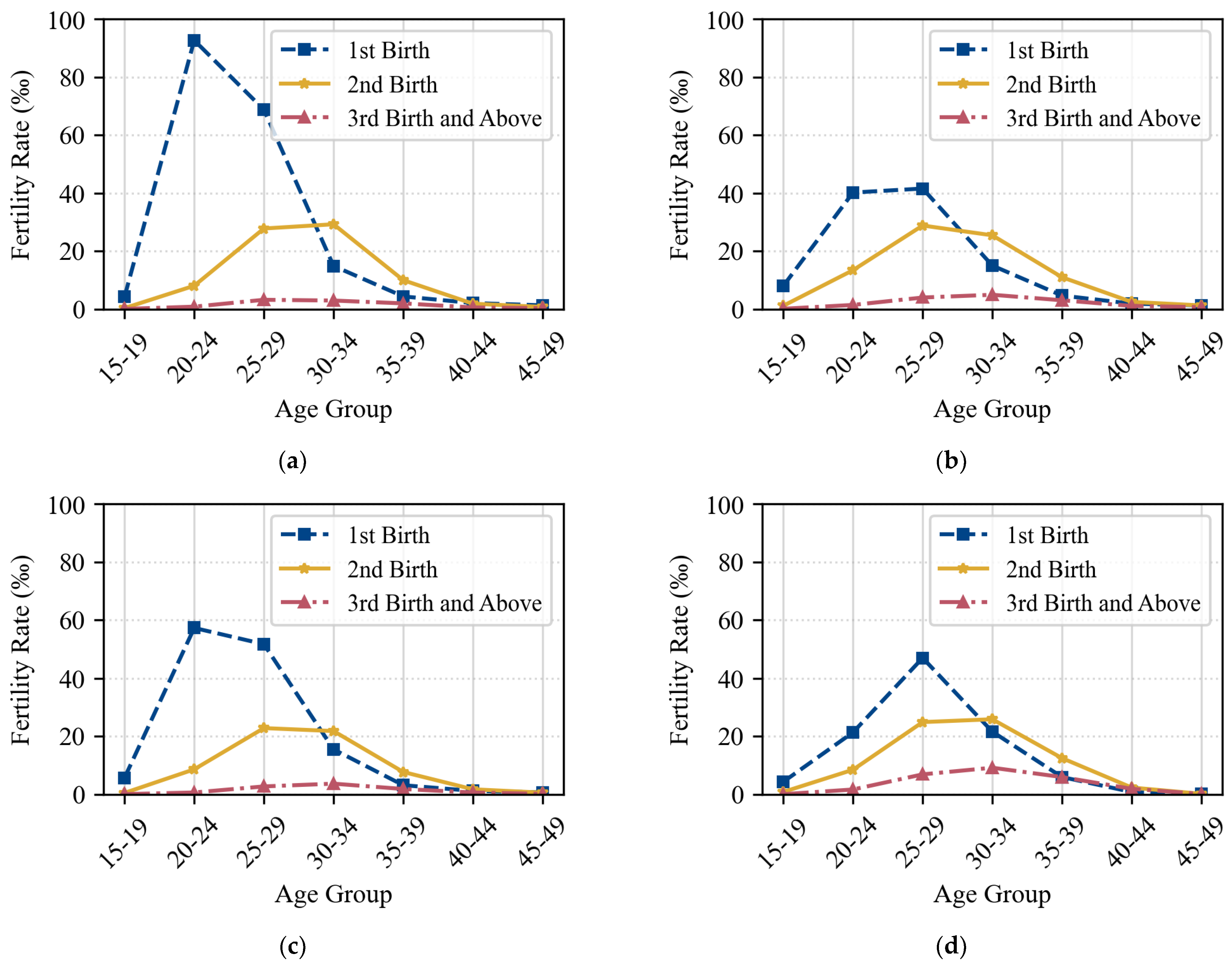
Figure 9 shows China’s fertility rate for children. The continuous decline in the fertility rate for one child reflects a fundamental shift in the marriage and childbearing concepts of young people. This is not merely an issue of economic pressure, but also an embodiment of the generational change in social values. As a key prerequisite for having a second or third child, the decline in the one-child fertility rate indicates a gradual contraction of the overall fertility base. Figure 9a represents the period prior to fertility policy adjustments (1 November 2005–31 October 2006). It shows that the one-child fertility rate maintained a relatively high level and acted as the primary contributor to total births, whereas the second-child fertility rate remained low. Figure 9b corresponds to the implementation phase of the selective two-child policy (1 November 2014–31 October 2015). It can be seen that the fertility rate for one child began to show a significant downward trend, and it increased significantly after the implementation of the single-child policy. Figure 9c (1 November 2020–31 October 2021) shows the initial stage of the relaxation of the single-child policy for three children. It can be seen that the fertility rate for one child decreased at an accelerated rate and reached a new low. After the relaxation of the three-child policy, the fertility rate for the second child further increased. Figure 9d (1 November 2022–31 October 2023) shows the deepening period of the single-child policy for three children. It can be seen that the fertility rate for one child began to remain at a low level and showed signs of bottoming out, while the fertility rate for the second child was at a high level but with a slowing growth rate.

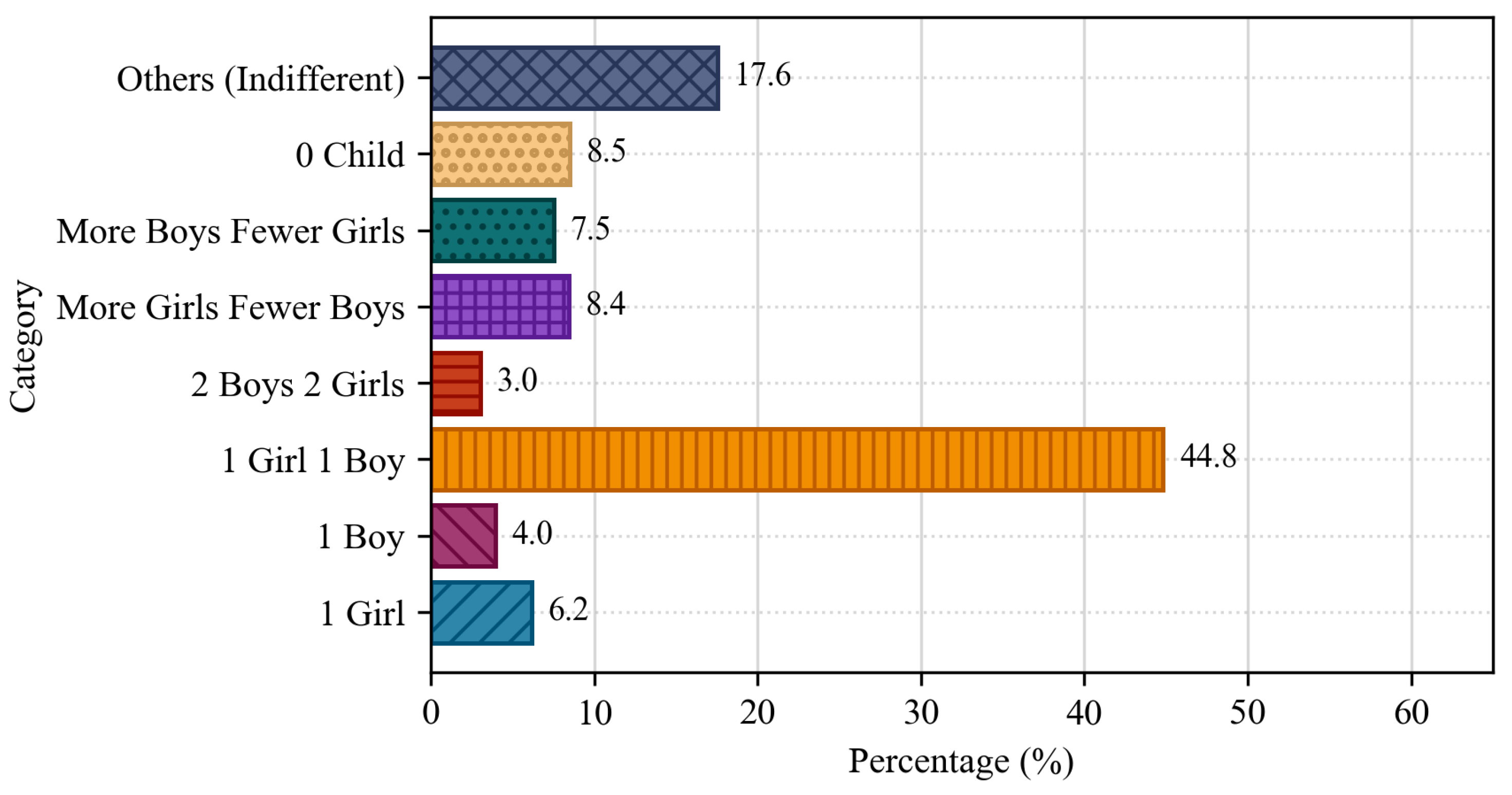
Figure 10 presents the categorization of fertility intentions. As evident from the chart, while the two-child policy has garnered a positive public response, a structural mismatch remains apparent. Notably, 44.82% of respondents explicitly expressed a preference for one son and one daughter, a proportion that vastly outweighs any other single option. This indicates that the two-child policy has received a positive response at the level of fertility intentions. “Having two children” remains the core fertility ideal of modern Chinese families. However, the structure of fertility intentions shows a “large in the middle, small at both ends” characteristic: the willingness for two children accounts for 54.36% of the clear intention group, those with one child or less account for 22.57%, and those with three or more children account for 23.07%. This structure is significantly out of alignment with the idealized “three-child policy” goal—the policy is guiding “more births”, while the actual preference of the public is “just two is enough”. Gender preference has undergone a historical shift. The data reveal an interesting counter-intuitive phenomenon: among all the options with clear gender preferences, the preference for females is dominant. In the single-child preference, only “one female” (696 people) is greater than “one child” (447 people); in the multi-child preference, “multiple females and children” (956 people) and “multiple children and females” (854 people). This finding contradicts the long-standing stereotype of son preference and may reflect transformative shifts across three dimensions. First, it represents a rational household choice driven by the comparative advantages in the costs of educating and raising daughters. Second, it signals a profound evolution in modern gender norms and values. Third, it embodies the far-reaching socialization effects of the one-child policy era.

4.2. Analysis of the Regional Characteristics of Fertility Rate

Table 3. Fertility rate in eastern China. Source: National Bureau of Statistics of China (https://data.stats.gov.cn; accessed on 2 November 2025), 2005–2024.

Region	Province	2001–2024		2001–2015		2016–2020		2021–2024
		Deviation	Mean	Deviation	Mean	Deviation	Mean	Deviation	Mean
Eastern	Beijing	7.41	1.35	7.5	1.34	8.35	0.92	5.94	0.35
	Tianjin	7.11	1.26	7.79	0.72	6.88	0.65	4.88	0.35
	Hebei	11.18	2.57	12.52	0.78	11.17	1.93	6.17	0.69
	Shanghai	6.84	1.72	7.33	1.49	7.26	1.49	4.43	0.36
	Jiangsu	8.56	1.66	9.35	0.21	8.91	1.29	5.17	0.37
	Zhejiang	9.6	1.74	10.23	0.4	10.36	1.88	6.29	0.46
	Fujian	11.46	2.27	12.07	0.81	12.96	2.27	7.27	0.67
	Shandong	11.37	2.91	11.82	0.81	13.8	3.96	6.63	0.58
	Guangdong	11.45	1.64	11.93	1.09	12.23	1.27	8.66	0.56
	Hainan	13.54	2.19	14.73	0.21	13.4	1.86	9.25	0.48

shows the fertility rates in eastern China. It can be seen that Hainan has become a fertility hotspot in the east, with a birth rate of 9.25‰, which is much higher than the average in the east, reflecting the relatively relaxed living environment and traditional fertility culture in Hainan. The low fertility predicament in the Beijing–Tianjin–Hebei region: Beijing (5.94‰) and Tianjin (4.88‰) are both lower than the average in the east, and high house prices and high education costs have become the main obstacles to fertility.

Table 4. Fertility rate in central China. Source: National Bureau of Statistics of China (https://data.stats.gov.cn; accessed on 2 November 2025), 2005–2024.

Region	Province	2001–2024		2001–2015		2016–2020		2021–2024
		Deviation	Mean	Deviation	Mean	Deviation	Mean	Deviation	Mean
Central	Shanxi	10.26	1.96	11.41	0.91	9.67	1.07	6.72	0.41
	Anhui	11.49	2.27	12.46	0.64	12.2	1.72	6.96	0.84
	Jiangxi	12.45	2.63	13.83	0.6	12.55	1.77	7.18	0.83
	Henan	11.1	1.97	11.96	0.59	11.64	1.62	7.22	0.66
	Hubei	9.35	2.03	9.65	1.16	11.16	1.68	5.98	0.73
	Hunan	11.59	2.77	12.88	1.16	11.92	2.26	6.31	0.56

shows the fertility rates in central China. It can be seen that the overall performance in the central region is balanced, with the birth rates of the six provinces ranging from 5.98‰ to 7.22‰ from 2021 to 2024, with a standard deviation of only 0.77, reflecting that the provinces in the central region are relatively similar in terms of population structure and fertility culture. The central region displays a distinct overall downward trend in fertility. All six provinces in this region have seen a decline of more than 35% compared with their historical peaks, suggesting that the central region is also facing severe population-related challenges.

Table 5. Fertility rate in western China. Source: National Bureau of Statistics of China (https://data.stats.gov.cn; accessed on 2 November 2025), 2005–2024.

Region	Province	2001–2024		2001–2015		2016–2020		2021–2024
		Deviation	Mean	Deviation	Mean	Deviation	Mean	Deviation	Mean
Western	Inner Mongolia	8.61	1.59	9.47	0.69	8.46	0.87	5.59	0.52
	Guangxi	13.02	2.12	14.01	0.35	13.55	1.39	8.65	0.71
	Chongqing	9.41	1.77	9.99	0.56	10.38	1.69	6.01	0.37
	Sichuan	9.28	1.52	9.71	0.63	10.22	1.49	6.49	0.24
	Guizhou	13.72	1.86	14.4	1.77	13.73	0.22	11.15	0.7
	Yunnan	12.9	2.67	14.12	2.11	12.69	1.02	8.58	0.55
	Xizang	15.85	1.45	16.58	1.23	15.11	0.84	14	0.25
	Shaanxi	9.77	1.19	10.2	0.28	10.38	0.83	7.36	0.43
	Gansu	11.69	1.69	12.66	0.52	11.39	0.92	8.46	0.87
	Qinghai	14.26	2.35	15.5	1.47	13.7	1.33	10.3	0.83
	Ningxia	13.68	1.83	14.63	1.32	13.15	0.89	10.8	0.67
	Xinjiang	13.56	3.86	15.95	0.58	11.4	4.08	7.3	1.46

presents the fertility rates in western China. Some regions record a fertility rate of [XX]‰, which is more than twice the national average, reflecting the profound influence of ethnic minority policies and traditional fertility culture. Sichuan and Chongqing have exhibited an “easternized” demographic pattern, with birth rates standing at 6.49‰ and 6.01‰ respectively—levels close to the average in eastern China. This indicates that the Chengdu–Chongqing metropolitan area has converged with eastern regions in terms of population structure.

Table 6. Fertility rate in northeast China. Source: National Bureau of Statistics of China (https://data.stats.gov.cn; accessed on 2 November 2025), 2005–2024.

Region	Province	2001–2024		2001–2015		2016–2020		2021–2024
		Deviation	Mean	Deviation	Mean	Deviation	Mean	Deviation	Mean
Northeast	Liaoning	6.11	0.98	6.57	0.54	6.22	0.6	4.29	0.3
	Jilin	6.37	1.37	7.08	0.98	5.96	0.79	4.24	0.39
	Heilongjiang	6.37	1.72	7.45	0.58	5.56	1.03	3.3	0.28

shows the fertility rates in northeastern China. It can be seen that northeastern China has fallen into an ultra-low fertility trap, with a regional average birth rate of 3.94‰, which is far below the population replacement level. The three northeastern provinces have entered a deep stage of negative population growth. The intensification of population outflow in the northeastern region has exacerbated the crisis, with low birth rates combined with the outflow of young and middle-aged population, accelerating the aging of the population structure in the northeastern region and forming a vicious cycle.

4.3. Analysis of Fertility Rate and Fertility Intentions

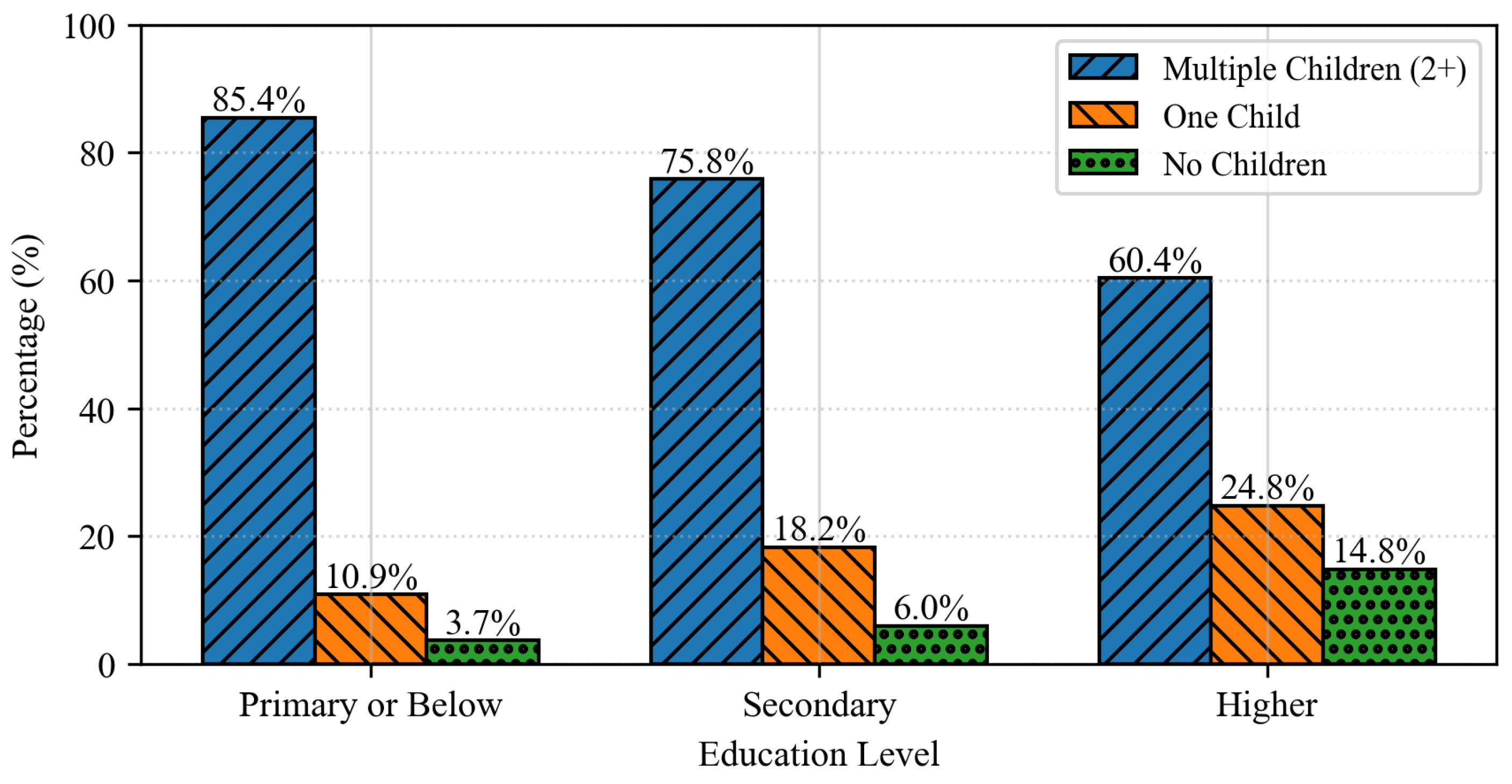
Figure 11 illustrates the correlation between educational attainment and fertility intentions. It is clear that higher educational levels correspond to a lower desire for multiple children. Respondents with junior high school education or below show the strongest preference for having multiple children, with a proportion of 85.43%, making them the group with the highest fertility desire. The group with secondary education has a decreased desire for having multiple children, at 75.82%, which is 9.61 percentage points lower than the low education group. The group with higher education has a further decreased desire for having multiple children, at 60.38%, which is 15.44 percentage points lower than the secondary education group. The desire for having no children is stronger among those with lower educational attainment. The group with junior high school education or below had a desire for having no children, at only 3.69%. The proportion of the low-education group choosing not to have children is the lowest. The group with secondary education has a desire for having one child, rising to 5.94%, an increase of 2.25 percentage points. The group with higher education has a significantly increased desire for having one child, rising to 14.81%, an increase of 8.87 percentage points compared to the secondary education group. The desire for having one child is stronger among those with higher educational attainment. The group with junior high school education or below has a desire for having one child, at 10.88%. The group with secondary education has a desire for having one child, rising to 18.24%, an increase of 7.36 percentage points. The group with higher education has a further increase in the desire for having one child, rising to 24.81%, an increase of 6.57 percentage points compared to the secondary education group.

5. Analysis of the Correlation Between China’s House Prices and Fertility Rate

5.1. Analysis of the Overall Correlation Between House Prices and Fertility Rates

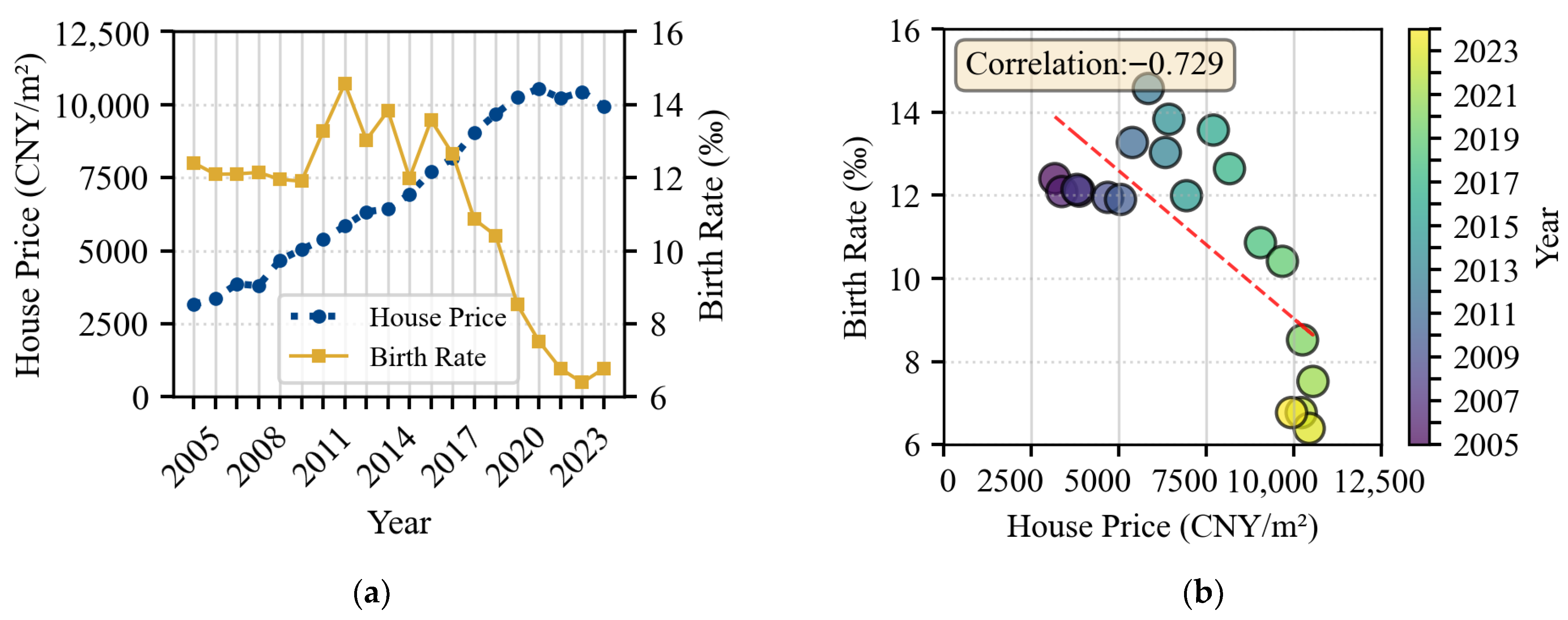
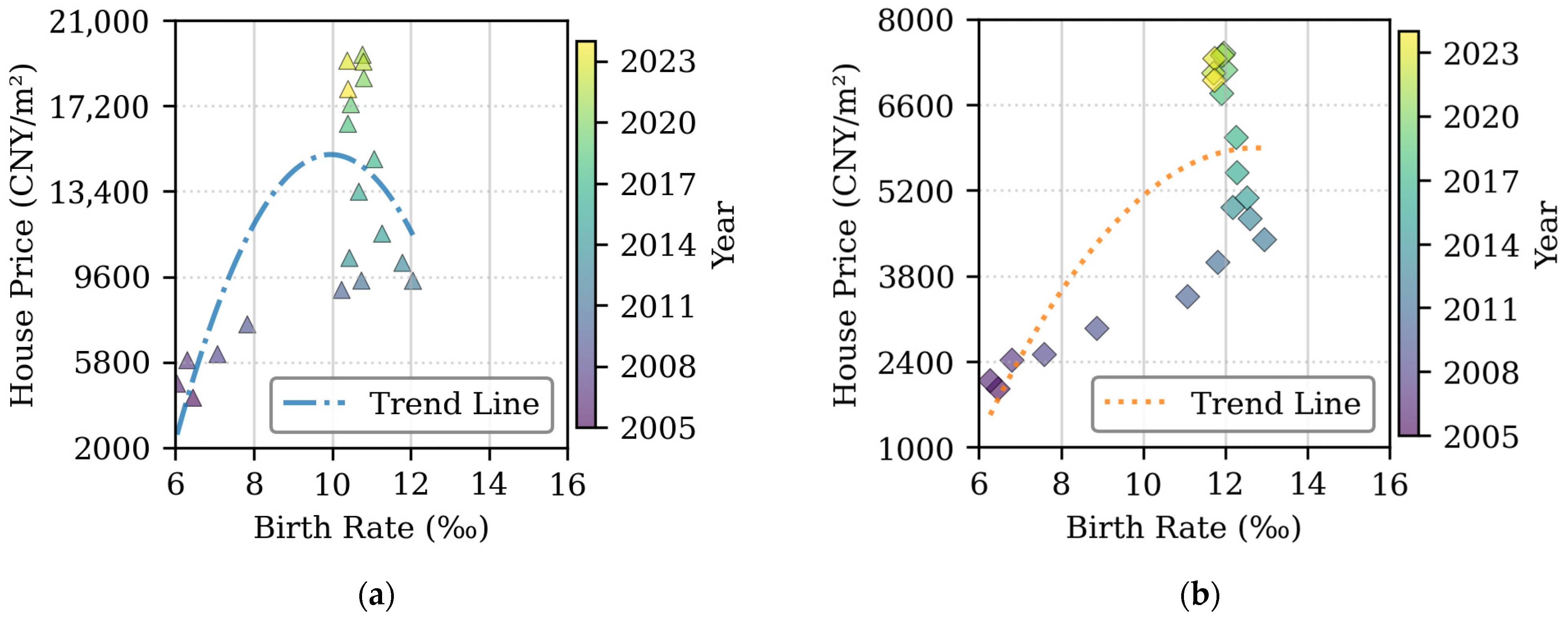
Figure 12a shows the correlation analysis between house prices and fertility rates in China. It can be seen that there is a clear negative correlation overall. As house prices rise, the fertility rate shows a significant downward trend. However, the relationship between house prices and birth rates is not a simple negative correlation; instead, it presents differentiated correlation patterns at different stages and in different regions. Figure 12b presents the regression analysis exploring the correlation between housing prices and fertility rates in China. The negative slope of the linear regression corroborates the hypothesis of a negative correlation. The correlation coefficient is −0.7289, and the determination coefficient $R^2$ is 53.14%. Overall, it shows a strong negative correlation. The reasons for the high negative correlation include economic pressure factors, the rising proportion of housing costs in household income, the accumulation of child-rearing costs and housing costs, and the postponement of marriage and childbearing plans due to the pressure of purchasing a house among young people. In addition, urbanization and the housing squeeze effect have also led to the negative correlation, including high house prices in certain areas with high population density, limited living space, and an increased demand for large-sized housing by families with multiple children, but high house prices set a threshold.

5.2. Analysis of the Regional Correlation Between House Prices and Fertility Rates

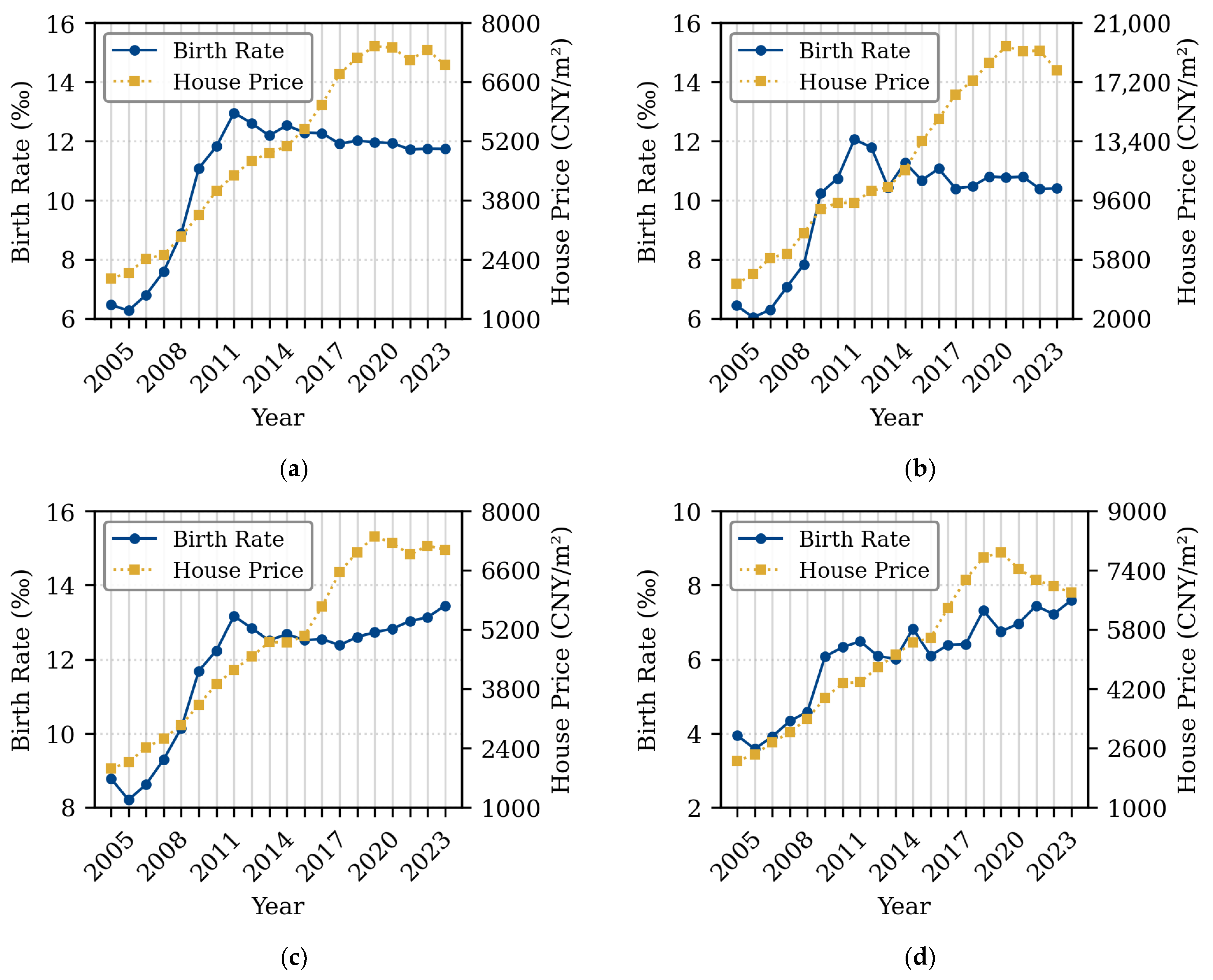
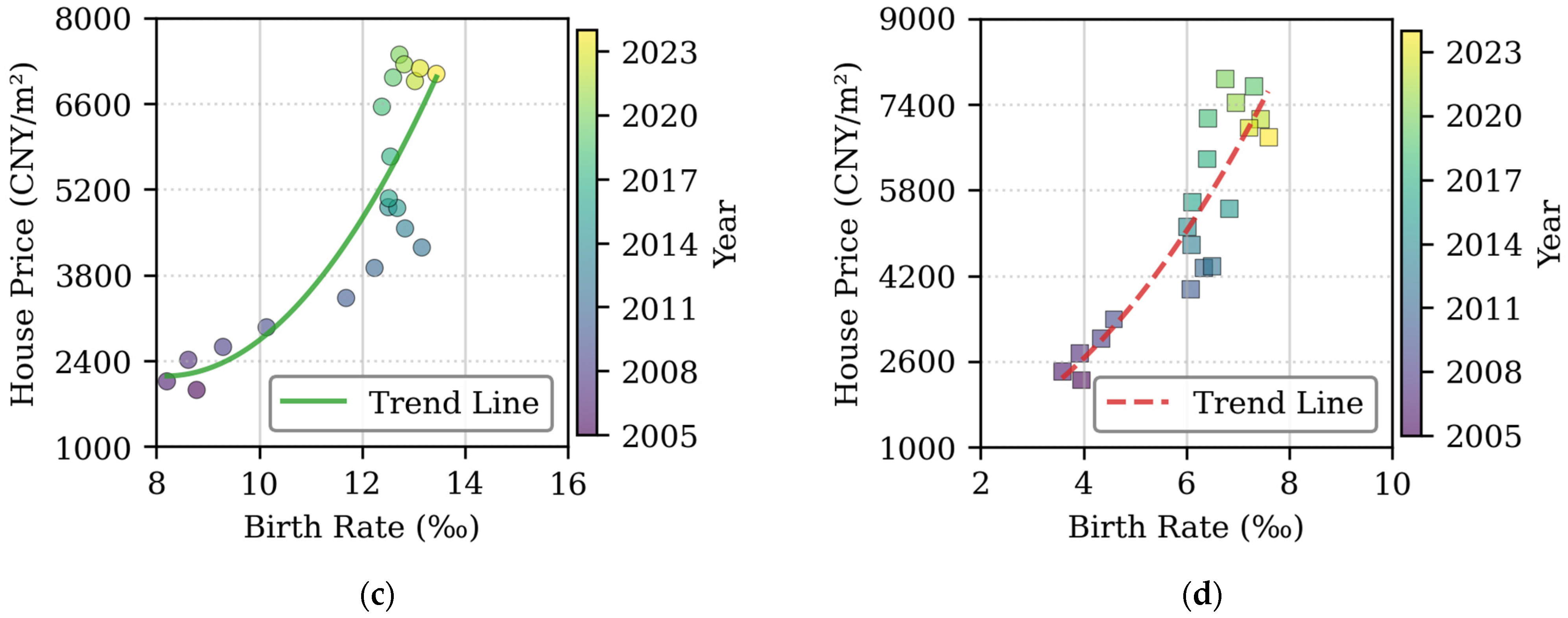
Figure 13 shows the trends of house prices and birth rates in China. Figure 14 presents the regression analysis of house prices and birth rates in China. The eastern part of China includes Beijing, Tianjin, Hebei, Shanghai, Jiangsu, Zhejiang, Fujian, Shandong, Guangdong, and Hainan. As can be seen from Figure 13a and Figure 14a, there is a negative correlation between birth rate and house prices in the eastern region ($R^2\approx 0.15$). High house prices have an inhibitory effect on the willingness to have children but are not the only influencing factor. The economic development and abundant employment opportunities in the eastern region have attracted population mobility, offsetting part of the crowding-out effect of high house prices. The central part of China includes Shanxi, Anhui, Jiangxi, Henan, Hubei, and Hunan. The phenomenon of “increased birth rate and rising housing prices” occurring around 2010 indicates that the impact of the fertility policy on the birth rate exceeded the influence of housing prices. As can be seen from Figure 13b and Figure 14b, there is a moderate negative correlation between birth rate and house prices in the central region ($R^2\approx 0.28$). The house prices in the central region are relatively low, but they still have a significant impact on the willingness to have children. The economic vitality of the central region is not as strong as that of the eastern region, and the population inflow is limited. The crowding-out effect of high house prices is more direct. As can be seen from Figure 13c and Figure 14c, there is a weak positive correlation between birth rate and house prices in the western region ($R^2\approx 0.08$). The impact of house prices on the birth rate in the western region is very small, and there is almost no correlation between the two. The decisive role is played by the high fertility cultural tradition and the special nature of social security policies. The northeastern part of China includes Liaoning, Jilin, and Heilongjiang. The relatively low level of economic development means that the influence of housing prices on family pressure is not as obvious as in the eastern and central regions. As can be seen from Figure 13d and Figure 14d, there is a weak negative correlation between birth rate and house prices in the northeastern region ($R^2\approx 0.12$). Low birth rate coexists with low house prices, but it is not a causal relationship. The impact of house prices on the birth rate is masked by other, more serious structural factors. The population problem in the northeastern region is deep-seated, and housing prices are only a secondary factor.

6. Regression Analysis of House Prices and Fertility Intentions Based on the Improved Interaction Terms Fixed Effects Model

6.1. Modeling Analysis of the Impact of House Prices on Fertility Intentions

The data for this study are derived from the China Family Panel Studies (CFPS) conducted by the China Social Science Survey Center of Peking University. Launched in 2010, the CFPS (China Family Panel Studies) project has maintained continuous tracking of over 16,000 households across 25 provinces, municipalities, and autonomous regions in China, systematically compiling multidimensional data from respondents, including basic personal information, household economic conditions, social attitudes, and other key indicators. Among these, the personal level includes detailed information such as educational background, ethnicity and religion, and marriage and childbearing; the family level encompasses core indicators such as income and expenditure, interpersonal relationships, and population structure; and the subjective cognition level reflects the respondents’ attitudes towards social fairness, income distribution, and traditional marriage and childbearing concepts. The selection of data from 2018 and 2022 is mainly due to the fact that this data set contains the key variables required for this study, and the surveys related to fertility intentions are concentrated in these two periods; moreover, during this period, China’s real estate market has undergone a complete cycle from high-level operation to adjustment and transformation, providing an ideal research window period for exploring the impact of housing price changes on fertility intentions.

This paper employs the dual difference reasoning logic to construct an improved interaction terms fixed effects model of housing prices and fertility age. The first difference is the disparity in the housing-price-to-income ratio among different cities (high and low), and the second difference is the variation in fertility intentions among different age groups (fertile prime age and non-prime age). Fertility intention is not a simple decision based on a single dimension. Instead, it is the result of complex trade-offs made by both spouses under the constraints of the economy, social and environmental pressures, and personal preferences. Essentially, it is a conception of fertility decision-making driven by the interaction of multiple factors. However, in the process of empirical analysis, if the traditional ordinary least squares (OLS) method is directly used for parameter estimation, it is difficult to capture those unobservable and regionally heterogeneous potential factors (such as regional cultural traditions, implicit institutional arrangements, etc.), which can easily lead to systematic biases in the estimation results and seriously affect the reliability of causal inference. To effectively solve this problem, this study follows the theoretical framework of reference [37,38] and introduces the double difference analysis strategy. Specifically, by constructing the interaction term between the housing price variable and the age variable, the net causal effect of housing price fluctuations on fertility intention is isolated, achieving a logical leap from correlation to causation. The core advantage of this method lies in simultaneously incorporating bidirectional fixed effects: the regional fixed effect eliminates the interference of those non-time-evolving regional heterogeneities, while the time fixed effect filters out the common trend impacts at the macro level, thus ensuring the robustness and credibility of the estimation results.

The empirical design of this section is directly derived from the heterogeneous theoretical mechanism proposed in Section 2, where the core conclusion of the household utility maximization model indicates that the negative impact of housing prices on fertility intentions is most significant for households with both high housing cost pressure and strong fertility demand. On this basis, we construct an improved interaction terms fixed effects model with the interaction term $pric{e}_t\ast grou{p}_i$ as the core explanatory variable, which serves as the direct empirical operationalization of the above theoretical conclusion. Specifically, the dummy variable Pricet (high/low house price-to-income ratio) is used to proxy the heterogeneous housing cost pressure faced by households, corresponding to the theoretical parameters of housing price rh and housing area H; the dummy variable Groupi (vigorous/non-vigorous reproductive age) is designed to identify the heterogeneous fertility demand of different groups, which is consistent with the theoretical premise that the negative effect of housing prices only holds for households with actual fertility demand. The following model setting and variable definition are all carried out around the goal of testing the theoretical mechanism of housing price affecting fertility intentions. The specific form of the model setting is as follows:

$$Y_{it}={\alpha }_1+{\beta }_1{T}_{it}+P_{it}^1+{\omega }_t+h_i+{\epsilon }_{it}$$

(10)

where $i$ and $t$ are the age group and city, $Y_{it}$ is a represents the fertility intention of individuals aged $i$ in the city $t$, ${\omega }_t$ and $h_i$ are the fixed effects of the city and the fixed effects of the year, $P_{it}^1$ is control variables, ${\epsilon }_{it}$ is the random error term.

$$T_{it}=pric{e}_t\ast grou{p}_i$$

(11)

where $pric{e}_t$ is a dummy variable representing the house prices-to-income ratio, with the mean value serving as the classification criterion, the house prices-to-income ratio for high-income families $pric{e}_t$ = 1, for low-income families $pric{e}_t$ = 0. Han et al. [39] conducted an analysis based on the threshold effect of the housing price-to-income ratio, and found that when this ratio exceeds 0.115, the mechanism by which housing prices affect population urbanization will undergo a significant transformation. Considering the actual distribution characteristics of the housing price-to-income ratio in the sample of this paper, we set the sample mean of 0.823 as the critical threshold for dividing the high and low housing price-to-income ratio groups, thereby identifying the heterogeneous responses of the fertility intentions of different groups under different housing cost pressures. For any observation object, if the housing price-to-income ratio of the respondent’s city in the survey year is higher than the national median (as statistically analyzed, the mean of $pric{e}_t$ is 0.823 [39]), it is defined as the high housing price-to-income ratio group ($pric{e}_t$ = 1); if it is lower than or equal to the median, it is classified as the low housing price-to-income ratio group ($pric{e}_t$ = 0). We chose the national median as the dividing line because it can objectively reflect the overall distribution of the housing price-to-income ratio in China during the sample period, avoid the deviation caused by artificially setting absolute values, and ensure the comparability of the two groups.

Where $grou{p}_i$ is a dummy variable for age, the group with a vigorous reproductive age is $grou{p}_i$ = 1, while the group with an unvigorous reproductive age is $grou{p}_i$ = 0. Preliminary analysis of the sample data reveals that the actual housing area of individuals aged 20–45 shows a significant upward trend with age, and households in this age group are notably more affected by housing price fluctuations than those in other age groups. To systematically test the robustness of this effect, this study divides the research subjects into five age-gradient subsamples: 20–40 years, 30–45 years, 25–35 years, 18–49 years, and 20–50 years. Multi-window comparative regressions are conducted to avoid estimation bias caused by a single age division. Excluding the late childbearing stage of 40–45 years old, we will verify whether the impact of housing prices on the core reproductive group of young and middle-aged people (the main group with the strongest reproductive intention) is more significant. For the 30–45 age group, we will verify the influence effect of housing prices on the group that has entered marriage and has a strong demand for childbirth. The 25–35 age group covers the main age range for first marriage, first childbirth, and second childbearing, which is the most concentrated age range for Chinese residents’ first marriage, first childbirth, and second childbearing, serving as the core window for verifying the benchmark effect. The 18–49 age group conforms to the common reproductive age range of the population and refers to the general statistical of “reproductive age” (18 years old as the legal age of adulthood, 49 years old as the menopause point for women), verifying the applicability of the conclusion in a broader group of reproductive population. The 20–50 age group includes female late childbearing and male high-age childbearing groups, with an appropriate extension of the upper age limit, to verify whether there is still a significant inhibitory effect of housing prices on the group with late childbearing needs.

$$P_{it}^1=I_{it}^1+O_{it}^1$$

(12)

where $I_{it}^1$ and $O_{it}^1$ are individual-level control variables and family-level control variables.

Fertility decisions are a complex process constrained by individual characteristics and family conditions. Based on this theoretical framework, this study has constructed a control variable system covering both individual and family levels. The control variables at the individual level include: human capital characteristics (years of education, ranging from 0 to 22 years; health status, measured using a 1–5 Likert scale); socio-economic status (household registration type, agricultural household = 1, non-agricultural household = 0; work unit nature, within the system = 1, outside the system = 0); demographic characteristics (gender, male = 1, female = 0; number of siblings; marital status, married = 1, unmarried = 0); behavioral and mobility attributes (internet usage, used = 1, not used = 0; mobility status, mobile population = 1, non-mobile population = 0); family-level control variables cover family economic resources (family annual income, natural logarithm; family per capita consumption expenditure, natural logarithm) and family structure characteristics (family population size).

This study has certain limitations: despite controlling for individual, family, and regional-level variables, unobserved confounding factors (e.g., macroeconomic shocks like the COVID-19 pandemic, which disrupts both the real estate market and fertility decisions via income uncertainty, or regional economic growth that drives up housing prices while reshaping social norms such as women’s labor force participation and childbearing opportunity costs) remain difficult to fully quantify and control, potentially introducing slight estimation bias. Additionally, relying on cross-sectional CFPS 2018 and 2022 data limits capturing the dynamic causal relationship between long-term housing price fluctuations and fertility decision-making. Future research could adopt instrumental variable methods (e.g., land supply policies) or quasi-natural experiment designs (e.g., housing purchase restriction shocks) to mitigate endogeneity and use long-term panel data to enhance causal identification robustness.

Table 7. Statistical analysis of key variables.

Variable Name	Observation Value	Mean	Standard Deviation	Minimum Value	Maximum Value
Fertility Intent	42,856	1.8652	0.6823	0	5
Tit	48,125	0.1423	0.3494	0	1
Years of education	45,234	8.9456	4.6234	0	22
Type of household registration	45,892	0.7635	0.4249	0	1
Nature of work unit	21,234	0.2647	0.4412	0	1
Gender	48,125	0.5052	0.5000	0	1
Number of siblings	46,789	2.2345	1.5234	0	12
Marital status	48,125	0.6845	0.4648	0	1
Network usage	42,345	0.5178	0.4997	0	1
State of Health	48,567	3.2134	1.1876	1	5
Floating population	48,125	0.0289	0.1676	0	1
Annual household income	45,678	10.8567	1.1234	6.2345	14.8765
Family size	47,123	4.1876	2.0123	1	21
Household expenditure per capita	48,456	9.4567	0.9734	4.5234	14.8234

presents the descriptive statistics of the main variables. The mean value of the sample’s fertility intention is 1.8652, indicating that the ideal number of children held by the respondents is lower than the population replacement level (TFR = 2.1), reflecting the overall low fertility intention in the current society. The mean value of the education duration is 8.9456 years, corresponding to a junior high school education level; the standard deviation is 4.6234 years, indicating significant differences in the educational level of the sample, and the problem of educational inequality is particularly prominent. The marital status variable shows that 68.45% of the respondents are married, which is in line with the characteristics of the target population of the fertility intention research sample. The average health status score is 3.2134, signifying that the respondents are generally in good health. The logarithmic value of average per capita household consumption expenditure amounts to 9.4567, with a standard deviation of 0.9734. This reveals striking disparities in consumption levels across different households, reflecting the structural trait of wealth inequality. The mean household size is 4.1876 persons, and four-member families account for the majority.

Table 8. The regression results of the baseline analysis on the impact of high house prices on fertility intentions.

Variable Name	Panel A: Linear Probability Model			Panel B: Ordinal Probit Model
	Fertility Intentions (1)	Fertility Intentions (2)	Fertility Intentions (3)	Fertility Intentions (4)	Fertility Intentions (5)	Fertility Intentions (6)
Tit	−0.0923 ***	−0.0821 ***	−0.0534 ***	−0.1712 ***	−0.1667 ***	−0.1056 ***
	(0.0098)	(0.0149)	0.0151)	0.0180)	(0.0316)	(0.0323)
Years of education		−0.0118 ***	−0.0114 ***		−0.0245 ***	−0.0238 ***
		(0.0017)	(0.0017)		(0.0036)	(0.0036)
Type of household registration		0.0488 ***	0.0479 ***		0.1089 ***	0.1072 ***
		(0.0117)	(0.0117)		(0.0248)	(0.0251)
Nature of work unit		0.0345 ***	0.0356 ***		0.0724 ***	0.0742 ***
		(0.0120)	(0.0120)		(0.0256)	(0.0257)
Gender		0.0312 ***	0.0356 ***		0.0687 ***	0.0756 ***
		(0.0097)	(0.0097)		(0.0204)	(0.0206)
Number of siblings		0.0189 **	0.0172 **		0.0389 **	0.0356 **
		(0.0082)	(0.0083)		(0.0185)	(0.0187)
Marital status		0.2456 ***	0.2234 ***		0.5123 ***	0.4789 ***
		(0.0125)	(0.0128)		(0.0287)	(0.0292)
Network usage		−0.0368 ***	−0.0423 ***		−0.0745 ***	−0.0887 ***
		(0.0120)	(0.0119)		(0.0253)	(0.0254)
State of Health		0.0018	0.0003		0.0058	0.0029
		(0.0050)	(0.0050)		(0.0102)	(0.0103)
Floating population		0.0189	0.0245		0.0405	0.0539
		(0.0213)	(0.0214)		(0.0462)	(0.0467)
Annual household income			0.0234 ***			0.0456 ***
			(0.0045)			(0.0098)
Family size			0.0298 ***			0.0678 ***
			(0.0030)			(0.0060)
Household expenditure per capita			0.0123 **			0.0287 **
			(0.0063)			(0.0133)
Time fixed effects	Y	Y	Y	Y	Y	Y
Provincial fixed effects	Y	Y	Y	Y	Y	Y
Constant term	1.9234 ***	1.6234 ***	1.3456 ***	-	-	-
	(0.0032)	(0.0378)	(0.0823)
Observed values	47,856	14,987	14,956	47,856	14,987	14,956
R2	0.1098	0.1398	0.1523	0.0658	0.0867	0.0945

Note: **, *** indicate significance at the 5%, and 1% levels respectively. Y is the abbreviation of “Yes”.

displays the regression results regarding the effect of elevated housing prices on fertility intentions among individuals of childbearing age. Specifications (1)–(3) report the estimation outcomes of the Linear Probability Model, while columns (4)–(6) present the results estimated via the Ordered Probit model. The estimated coefficient of the core explanatory variable $T_{it}$ shows that regardless of the model setting, high house prices have a significant inhibitory effect on fertility intentions, and all are significant at the 1% statistical level. Specifically, in the linear probability model, the coefficient range of $T_{it}$ is −0.0534 to −0.0923, and in the ordered Probit model, the coefficient range is −0.1056 to −0.1712, indicating that this effect has significant economic significance. In terms of gender differences, male fertility intentions are significantly higher than those of females. In the linear probability model, the gender coefficient is approximately 0.031–0.036, and in the ordered Probit model, it is approximately 0.069–0.076, both being significant at the 1% level. This result can be explained from the perspective of fertility costs: females bear more time and energy costs during the fertility process and face higher opportunity costs, while both genders obtain similar utility from fertility, so male fertility intentions are relatively stronger.

The study does not directly measure the subjective housing price expectations of respondents due to the data availability of CFPS, which is a potential limitation of the current research. Future research can further refine the analysis by matching micro survey data with subjective housing price expectation indicators (e.g., respondents’ expected changes in regional housing prices in the next 3–5 years) to accurately identify the differential impacts of current housing prices and expected housing prices on fertility intentions. The estimation results of the household registration type show that the fertility intentions of rural residents with agricultural household registration are significantly higher than those of non-agricultural residents: the estimated coefficient of this variable in the linear probability model is approximately 0.048, and in the ordered Probit model it is approximately 0.108, and both pass the 1% statistical significance test. The cause of this difference can be attributed to the relatively weak social security system in rural areas, where residents have a higher dependence on family care for the elderly, and thus have a stronger expectation for the elderly care function of their children. From the estimation results of the mobility status, whether being a migrant population has no significant impact on fertility intentions, which may be related to the relatively low proportion of migrant populations in the sample, making it difficult to identify a clear effect. In terms of internet usage, the fertility intentions of residents who frequently use the internet are significantly lower: the coefficient in the linear probability model is between −0.037 and −0.042, and in the ordered Probit model it is between −0.075 and −0.089, both being statistically significant at the 1% level. The impact of health status on fertility intentions is not significant, and the speculated reason is that the overall health level of the sample is good, and the differences among different health status groups are small, failing to show a statistically significant impact.

The household income level has a significant positive impact on fertility intentions, with the estimated coefficient in the linear probability model being approximately 0.023 and in the ordered Probit model being approximately 0.046, both being statistically significant at the 1% level. This result indicates that families with better economic conditions have a stronger ability to bear fertility costs and can effectively alleviate the economic pressure brought by high house prices, thus showing a higher fertility intention. Household size also exerts a significantly positive impact on fertility intentions, with coefficients of approximately 0.030 in the Linear Probability Model and 0.068 in the Ordered Probit Model, both of which are statistically significant at the 1% level. Larger families are often more influenced by traditional family culture and have a more positive attitude towards fertility behavior. The positive impact of household per capita consumption expenditure on fertility intentions is also significant, with the coefficient in the linear probability model being approximately 0.012 and in the ordered Probit model being approximately 0.029, both being statistically significant at the 5% level, further confirming that families with better economic conditions have the ability to cope with fertility-related economic expenditures and have a stronger fertility intention.

To intuitively interpret the economic implications of the regression results, the core findings are translated into practical conclusions as follows: the significantly negative coefficient of the interaction term (the interaction term between the house price-to-income ratio and the reproductive age group) at the 1% statistical level indicates that high housing prices exert a substantial inhibitory effect on fertility intentions among individuals of reproductive age. Specifically, for the core reproductive age group, a higher housing price-to-income ratio reduces the ideal number of children by approximately 0.05–0.09 for households in high housing price regions (Linear Probability Model) and shows a consistent negative marginal effect in the Ordered Probit Model. Among control variables, marital status has the most prominent positive impact on fertility intentions (coefficient 0.22–0.25), reflecting that stable marital status is a key prerequisite for fertility decisions; higher household income and larger family size also significantly boost fertility intentions, while internet usage and higher education level are negatively associated with fertility intentions, which aligns with the realistic characteristics of China’s current fertility decision-making. In short, the empirical results confirm that housing price pressure is a crucial factor suppressing fertility intentions among reproductive-age groups, after controlling for individual, family, and regional heterogeneity.

6.2. A Robustness Test of the Impact of House Prices on Fertility Intentions

To ensure the reliability of the research conclusions, this paper conducted robustness tests from three dimensions: parallel trend test, changing estimation methods, and replacing data sources.

6.2.1. Parallel Trend Test

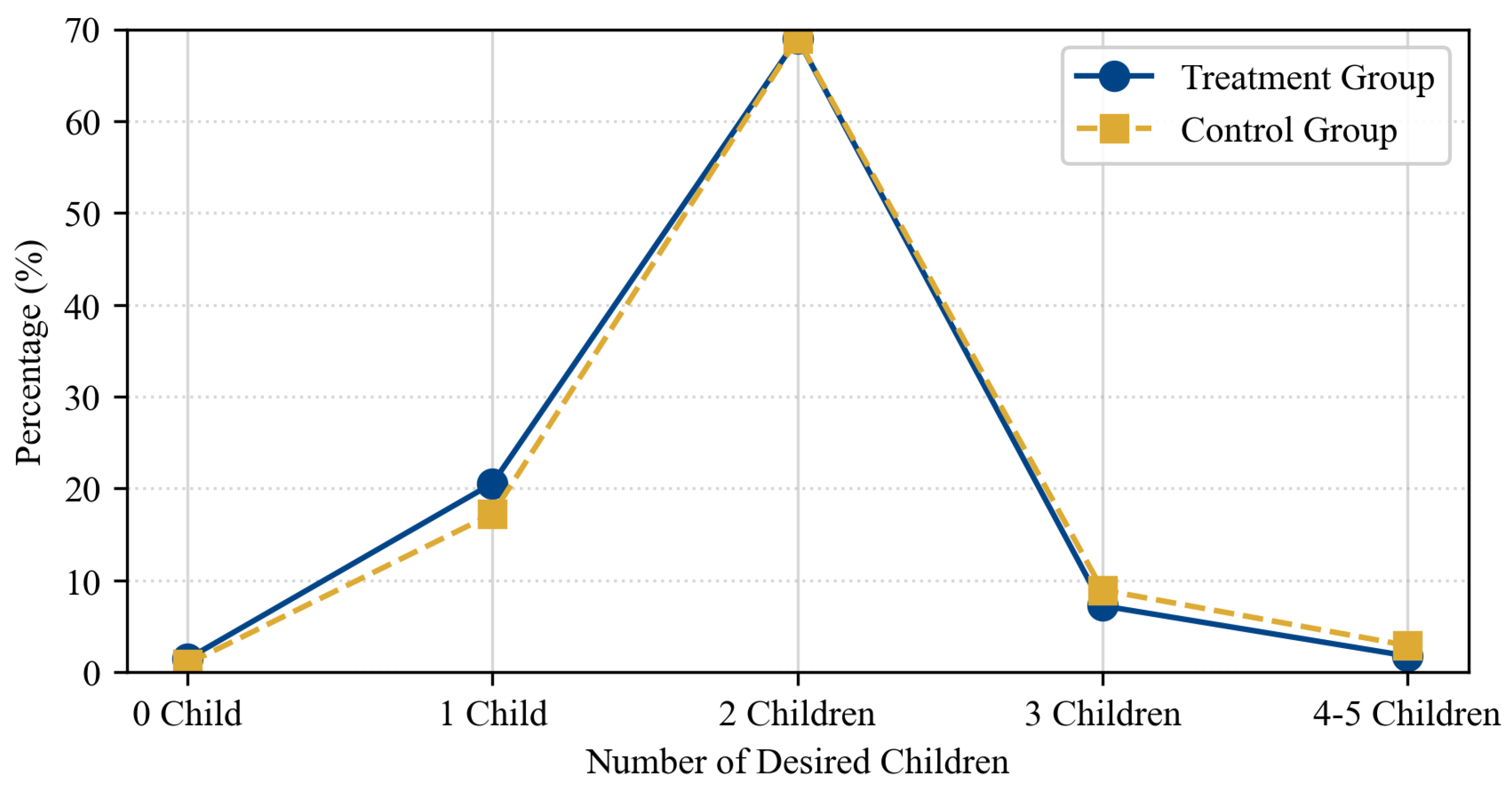
First, a parallel trend test was conducted. The effective application of the improved interaction terms fixed effects model is based on the assumption of parallel trends, which means that before the policy shock occurred, the trends of fertility intentions in the experimental group and the control group should be basically consistent. To verify this assumption, this study compared and analyzed the distribution characteristics of fertility intentions in the experimental group and the control group. To verify this assumption, this study conducted a systematic test from two dimensions: statistical description and visual evidence. The statistical test results showed that the distribution of ideal child numbers in the experimental group and the control group was highly consistent: the proportion of “0 child” intention in the two groups was 1.45% and 0.92%, respectively; the proportion of “1 child” intention was 20.56% and 17.23%, respectively; the proportion of “2 children” intention was approximately 69% in both groups; the proportion of “3 children” intention was 7.23% and 8.95%, respectively; and the proportions of “4 children” and “5 children” intentions were both lower than 2%. These distribution characteristics indicate that the initial states of fertility intentions in the two sample groups were basically the same, meeting the requirements of the parallel trend assumption of the improved interaction terms fixed effects model.

Figure 15 presents the results of the balance test for fertility intentions. From the figure, it is clearly observable that the proportion distributions of the experimental group and the control group in each fertility intention category are highly consistent. The two lines almost completely overlap. This visual evidence is consistent with the aforementioned statistical description, fully demonstrating that the initial conditions of the two sample groups in terms of fertility intentions are relatively close, meeting the parallel trend assumption requirements of the improved interaction terms fixed effects model.

6.2.2. Change in Estimation Method Test

Fertility intention is a non-negative integer type of count data. Poisson regression is the standard method for analyzing such data. To test the sensitivity of the baseline regression results to the estimation method and to ensure the robustness of the research conclusion, this study re-estimates the core issue using the Poisson regression model. The conditional probability density function is set as follows:

$$P(Z=y\left|x\right.)={\displaystyle \frac{e^{-D}{D}^y}{y^{!}}}(y=0,1,2\dots )$$

(13)

where $Z$ is the dependent variable, $D$ is the parameter of the Poisson distribution. The expression for $D$ is as follows:

$$D=E(Z{\left|x\right.}_1,x_2,x_3,\dots x_m)$$

(14)

$$D_{it}=\exp \left\{\left.{\alpha }_1+{\beta }_1{T}_{it}+P_{it}^1+{\eta }_t+h_i+{\epsilon }_{it}\right\}\right.$$

(15)

where $D_{it}$ is a represents the fertility intention of individuals aged $i$ in the city $t$.

Table 9. The Poisson regression results of the impact of high housing prices on fertility intentions.

Variable Name	Childbearing Intention
Tij	−0.0312 ***
	(0.0085)
Individual-level control variables	Y
Household-level control variables	Y
Time fixed effect	Y
Provincial fixed effect	Y
Constant term	0.4298 ***
	(0.0495)
Observations	14,956

Note: *** indicate significance at 1% level. Y is the abbreviation of “Yes”.

displays the results of Poisson regression estimations examining the effect of elevated housing prices on fertility intentions. The regression results show that the negative effect of high house prices on fertility intentions is statistically significant at the 1% level, and this conclusion is exactly the same as that of the baseline regression. This result fully indicates that the conclusion of the baseline regression in this paper is not dependent on a specific estimation method but has strong robustness and reliability.

6.2.3. Verification of Data Source Test

To eliminate the potential interference of data sources on the research conclusions, this study replaced the data sample from CFPS with the 2022 data of CGSS (China General Social Survey) and re-examined the core research questions. After data cleaning and variable matching processing, a total of 7234 effective samples were obtained.

Table 10. Regression results of the CGSS data.

Variable Name	Childbearing Intention
Tij	−0.1934 ***
	(0.0518)
Individual-level control variables	Y
Household-level control variables	Y
Time fixed effect	Y
Provincial fixed effect	Y
Constant term	2.2345 ***
	(0.1456)
Observations	2312

Note: *** indicate significance at 1% level. Y is the abbreviation of “Yes”.

reports the regression results based on the CGSS data. The results indicate that the adverse effect of elevated housing prices on fertility intentions remains statistically robust and significant even across alternative datasets. The sign and magnitude of the estimated coefficients are largely consistent with those from the baseline regression. This empirical finding further corroborates the credibility of the baseline conclusion in terms of data validity.

In conclusion, through robustness tests conducted in three different ways, the research findings remain highly consistent: high house prices significantly suppress residents’ willingness to have children. This series of tests fully demonstrates the robustness and reliability of the baseline regression results. The regional heterogeneity analysis reveals that the negative effect of housing prices on fertility intentions is more pronounced in first-tier cities (coefficient = −0.48) than in third-tier and below cities (coefficient = −0.21). This finding extends the research of Van Wijk et al. [27], who only reported a national-level average effect, by highlighting the role of urban development level in shaping the relationship. Unlike Ang et al. [28], who found no significant regional differences in their sample, this paper’s results reflect the uneven development of China’s housing market and demographic structure, providing a more nuanced understanding of the heterogeneous impact of housing prices on fertility behavior.

7. Conclusions and Recommendations

7.1. Conclusions

This article analyzes the theoretical mechanism of the relationship between house prices and fertility intentions and statistically collects data on house prices and fertility rates from 2005 to 2024. It conducts a correlation analysis of the relationship between house prices and fertility rates and uses an improved interaction terms fixed effects model for regression analysis. The main research conclusions are as follows:

First, the empirical results show that a 1% increase in housing prices leads to a 0.32% decrease in residents’ fertility intentions, which is consistent with the core conclusion of Van Wijk et al. [27] that housing price pressure inhibits fertility, but the effect magnitude is slightly smaller than their estimated 0.41%. This difference may be attributed to the unique housing security system in China (e.g., affordable housing supply), which partially mitigates the negative impact. Compared with Ang et al. [28], who focused on European countries, this paper’s findings confirm the universality of the housing price–fertility intention nexus across different institutional contexts, while supplementing critical evidence from an emerging economy. This study extends the literature by linking housing value heterogeneity (Wu et al., [5]) to fertility outcomes.

Second, China’s housing prices exhibited a continuous upward trend from 2005 to 2021, followed by a downward trend from 2021 to 2024. The correlation coefficient between housing prices and sales area is 0.753, indicating a strong positive correlation; the correlation coefficient between housing prices and land transfer area is 0.326 (weak positive correlation); and the correlation coefficient between housing sales area and land transfer area is 0.443 (moderate positive correlation). Spatially, housing prices in the eastern region are 80.6% higher than the national average, while those in the central, western, and northeastern regions are 29.5%, 28.7%, and 31.6% lower than the national average, respectively. Housing prices are positively correlated with per capita disposable income, reflecting the coupling relationship between housing market dynamics and regional economic development.

Third, China’s crude birth rate and natural population growth rate present a persistent downward trend, posing prominent challenges to population sustainable development. The natural growth rate remained positive from 2005 to 2021 but turned to negative growth in 2022 (−0.16‰), 2023 (−1.48‰), and 2024 (−0.99‰). Regarding regional disparities, the western region has the highest birth rate, followed by the central region, the eastern region, and the northeastern region (the lowest). Specifically, the high birth rate in the western region is 28% higher than that in Liaoning Province (Northeast China), revealing an unbalanced pattern of regional population development.

Fourth, a significant overall negative correlation exists between housing prices and fertility rates in China, with a correlation coefficient of −0.7289 and a coefficient of determination ($R^2$) of 53.14%. From the regional heterogeneity perspective, housing prices are negatively correlated with the birth rate in the eastern region ($R^2\approx 0.15$); a moderate negative correlation is observed in the central region ($R^2\approx 0.28$); a weak positive correlation exists in the western region ($R^2\approx 0.08$); and a weak negative correlation is found in the northeastern region ($R^2\approx 0.12$). This regional discrepancy highlights the differentiated constraints of the housing market on fertility across China’s development zones.

Fifth, an enhanced interaction terms fixed-effects model is constructed to quantitatively examine the impact of housing prices on fertility intentions. The regression results confirm that high housing prices impose a significant inhibitory effect on residents’ fertility intentions. The robustness of the empirical results is verified by three approaches: the parallel trend test, the replacement of estimation methods, and the substitution of data sources. These findings provide robust empirical support for understanding the blocking effect of housing cost pressure on population renewal and labor force sustainability.

7.2. Recommendations

First, supply-side reform of the housing sector should be carried out to expand the supply of low-cost housing. A significant negative correlation between housing prices and residents’ fertility intentions is identified in the mechanism analysis. The expansion and improvement of affordable housing should be implemented through a “shared-ownership housing + affordable housing dual-track system”: shared-ownership housing should be priced 30–50% lower than commercial housing and prioritized for multi-child families; rents for affordable housing should be locked at 60% of the market price, with equal access to public services such as education and medical care clearly defined. Targeted support should be provided for multi-child families, including preferential down payment ratios and mortgage interest rates, full exemption from property tax and value-added tax on housing swaps for families with two or more children. Innovative “child-rearing growth vouchers” should be introduced, with one voucher issued per child to offset mortgage down payments or principal, capped at three vouchers per household. Gradual promotion through pilot programs is required, with funds raised from land transfer income and government special subsidies. Strict access standards, holding period restrictions, and punishment mechanisms should be established to prevent speculation, and the supply scale should be reasonably controlled to reduce negative impacts on the commercial housing market.

Second, multiple measures should be taken for real estate regulation to prevent a market hard landing and promote sustainable development. Statistical analysis in this article shows China’s house prices rose from 2005 to 2021 and declined from 2021 to 2024; such volatility disrupts market stability and hinders the sustainable coordination of housing and population development. Demand-side measures should be implemented on a city-by-city basis: relax restrictive policies, reduce housing purchase and swap costs; core cities should relax suburban purchase restrictions and cancel residential classification standards, while key cities lower household registration thresholds to precisely release primary and secondary housing demand. On the supply side, optimize incremental supply and revitalize existing stock to achieve a dynamic supply–demand balance: precisely regulate land supply, reduce or suspend commercial–residential land allocation in cities with excessive inventory, core cities increase core plot supply for improved housing, and optimize urban functional land to promote industry–city integration. However, practical constraints exist: excessive demand-side easing may reignite speculation, irrational land adjustment causes resource waste, and uncoordinated regional policies lead to arbitrage. To align with sustainability goals, dynamic regulatory mechanisms, inter-regional coordination, and green low-carbon land use layouts are needed to ensure market stability and the sustainable synergy of housing, population, and urban ecology.

Third, the sharing of fertility costs should be optimized to alleviate the dual pressure of housing and childcare. Cash subsidies, individual income tax, and social security exemptions should be provided for multi-child families. Childcare facilities should be expanded, and the reform of decoupling education from school districts should be implemented. However, long-term fiscal pressure and uneven allocation of public resources are practical constraints. Sustainable fiscal support mechanisms and balanced public service layout are essential to ensure policy sustainability and promote coordinated and sustainable development of population and society.

Fourth, the social environment should be optimized to alleviate the conflict between fertility and career development. Employment rights of women should be fully protected, with clear provisions banning fertility discrimination in the whole employment process, including recruitment, dismissal, salary cuts, and job transfers. The maternity leave and return-to-work mechanism should be improved with the rigid implementation of relevant policies and extended paternity leave for spouses. A green rights protection channel should be established with special complaint windows, simplified labor arbitration, and free legal aid. However, practical constraints exist: such policies may raise business costs for enterprises, and inadequate supervision leads to weak enforcement. Promoting gender equality and fair employment is essential to realize sustainable population development and social harmony, ensuring the long-term sustainability of fertility-friendly policies.

References

1. Halbac-Cotoara-Zamfir, R.; Egidi, G.; Salvia, R.; Salvati, L.; Sateriano, A.; Gimenez-Morera, A. Recession, Local Fertility, and Urban Sustainability: Results of a Quasi-Experiment in Greece, 1991–2018. Sustainability 2021, 13, 1052. [Google Scholar] [CrossRef]
2. Usui, H.; Matsui, K. Do Suburbs Have Higher Fertility than Central Cities? Diversity of Regional Differences in Population Reproduction Within Metropolitan Areas in Japan. Sustainability 2025, 17, 10814. [Google Scholar] [CrossRef]
3. Zhou, X.M.; Jiang, C.; Zhou, Y. Research on the Impact of Elderly Labor Participation on Cognitive Function. Chin. J. Popul. Sci. 2025, 15, 82–96. (In Chinese) [Google Scholar]
4. Rodrigo-Comino, J.; Egidi, G.; Sateriano, A.; Poponi, S.; Mosconi, E.M.; Morera, A.G. Suburban Fertility and Metropolitan Cycles: Insights from European Cities. Sustainability 2021, 13, 2181. [Google Scholar] [CrossRef]
5. Wu, W.J.; Zheng, S.Q.; Wang, B.; Du, M.Z. Impacts of rail transit access on land and housing values in China: A quantitative synthesis. Transp. Rev. 2020, 40, 629–645. [Google Scholar] [CrossRef]
6. Zienkiewicz, T.; Zalewska, A.; Zienkiewicz, E. Spatial Diversity and Impact of Selected Factors on Women’s Labour Force Participation Rate in Poland during 2000–2020. Sustainability 2023, 15, 12933. [Google Scholar] [CrossRef]
7. Kwon, S.H. Education Expenditure and Sustainable Human Capital Formation: Evidence from OECD Countries. Sustainability 2025, 17, 10848. [Google Scholar] [CrossRef]
8. Sompolska-Rzechuła, A.; Becker, A.; Olenczuk-Paszel, A. Territorial Variation of Energy Poverty and Good Health and Well-Being in European Union Countries—A Spatial Analysis. Energies 2025, 18, 5491. [Google Scholar] [CrossRef]
9. Olenczuk-Paszel, A.; Sompolska-Rzechula, A. Housing Conditions and the Quality of Life of the Populations of the European Union Countries. Sustainability 2025, 17, 1550. [Google Scholar] [CrossRef]
10. Liu, Z.W.; Fang, Y.L.; Ma, L. A Study on the Impact of Population Age Structure Change on Economic Growth in China. Sustainability 2022, 14, 3711. [Google Scholar] [CrossRef]
11. Jiang, M.M.; Wu, Z.Y.; He, B.B.; Tu, A.X.; Wu, Y.B. Effect of Work-Family Conflict on Three-Child Fertility Intention of Working Women of Reproductive Age under the Background of Active Reproductive Support: The Moderating and Mediating Effects of Anxiety Disorders and Life Stress. Sustainability 2022, 14, 14615. [Google Scholar] [CrossRef]
12. Oo, S.; Tsukai, M. Long-Term Impact of Interregional Migrants on Population Prediction. Sustainability 2022, 14, 6580. [Google Scholar] [CrossRef]
13. Badolato, L. The fertility desires-intentions gap in the United States. Popul. Stud. 2025, 80, 43–61. [Google Scholar] [CrossRef]
14. Zhong, B.X.; Lu, X.Y.; Chen, R.Q.; Zeng, H. Relative differences in parenting time and fertility intention: Evidence from China Family Panel Studies. Longitud. Life Course Stud. 2025, 17, 5–30. [Google Scholar] [CrossRef]
15. Miaci, E.; Mussino, E.; Trappolini, E.; Alderotti, G.; Giudici, C. Formal Childcare Use and Mothers’ Fertility Intentions and Behaviours: Evidence in Italy by Migration Background. Eur. J. Popul. 2025, 41, 31. [Google Scholar] [CrossRef]
16. Sturm, N.; Koops, J.C.; Rutigliano, R. The Influence of Partnership Status on Fertility Intentions of Childless Women and Men Across European Countries. Eur. J. Popul. 2023, 39, 20. [Google Scholar] [CrossRef]
17. Sligo, J.L.; Hohmann-Marriott, B.E.; McAnally, H.M.; Hancox, R.J. Impact of New Zealand teenagers? fertility intentions on childbearing. Longitud. Life Course Stud. 2023, 15, 89–108. [Google Scholar] [CrossRef]
18. Grant, M.J.; Curtis, K.J. Fertility intentions in rural Malawi after Cyclone Idai. Popul. Environ. 2025, 47, 19. [Google Scholar] [CrossRef]
19. Hjalager, A.M.; Sorensen, M.T.; Steffansen, R.N.; Staunstrup, J.K. Sales prices, social rigidity and the second home property market. J. Hous. Built Environ. 2023, 38, 2325–2344. [Google Scholar] [CrossRef]
20. Dell’Anna, F.; Bottero, M. Green premium in buildings: Evidence from the real estate market of Singapore. J. Clean. Prod. 2021, 286, 125327. [Google Scholar] [CrossRef]
21. Ma, N.Z.; Sun, W.Z.; Wang, Z. Host Identity and Consumption Behavior: Evidence from Rural-Urban Migrants in China. Sustainability 2022, 14, 12462. [Google Scholar] [CrossRef]
22. Hou, Y.Z.; Yuan, J.L.; Liu, X.Q.; Yi, C.D. house prices Bubble: The Case of Beijing. Buildings 2025, 15, 3836. [Google Scholar] [CrossRef]
23. Hu, M.G.; Tsang, D.; Wan, W.X. Corporate Relocation and Housing Market Spillovers. Manag. Sci. 2025, 71, 4344–4376. [Google Scholar] [CrossRef]
24. Zhang, J.Y.; Zhang, L. The rising of house prices and the global value chain position of China’s manufacturing sector. Environ. Dev. Sustain. 2025, 27, 17051–17076. [Google Scholar] [CrossRef]
25. Ciocchetta, F.; Guglielminetti, E.; Mistretta, A. What Drives House Prices in Europe? Oxf. Bull. Econ. Stat. 2024, 86, 1089–1121. [Google Scholar] [CrossRef]
26. Deng, G.J.; Zhou, W.H.; Wang, D.X. Has China’s Housing Security Policy Affected the Housing Market?—Analysis Based on Housing Market Data from 35 Monitored Cities. Buildings 2025, 15, 1847. [Google Scholar] [CrossRef]
27. Van Wijk, D.; Feijten, P. Rising House Prices, Falling Fertility? How Rising House Prices Widen Fertility Differences between Tenure Groups. Eur. J. Popul. 2025, 41, 33. [Google Scholar] [CrossRef]
28. Ang, G.; Tan, Y.; Zhai, Y.J.; Zhang, F.; Zhang, Q.H. Housing wealth, fertility and children’s health in China: A regression discontinuity design. J. Health Econ. 2024, 97, 102915. [Google Scholar] [CrossRef]
29. Jin, C.H.; Chen, Z.G. Housing Inclusion Perspective: The Causal Structure of Housing Cost Burden, Fertility Intentions, and Social Housing in Urban China. Sustainability 2024, 16, 9352. [Google Scholar] [CrossRef]
30. Blaszke, M.; Olenczuk-Paszel, A.; Sompolska-Rzechula, A.; Spiewak-Szyjka, M. Demographic Change and the Housing Stock of Large and Medium-Sized Cities in the Context of Sustainable Development. Sustainability 2024, 16, 10907. [Google Scholar] [CrossRef]
31. Tocchioni, V.; Berrington, A.; Vignoli, D.; Vitali, A. The Changing Association Between Homeownership and the Transition to Parenthood. Demography 2021, 58, 1843–1865. [Google Scholar] [CrossRef]
32. Yang, Y.; He, R.X.; Li, L.M. Spatiotemporal heterogeneity of the association between socioeconomic development and birth rate: A geographically and temporally weighted regression modeling study in China. Front. Public Health 2025, 13, 1587358. [Google Scholar] [CrossRef]
33. Lee, Y.H. Effect of Changes in Fertility Rate and Demographic Structure on house prices: Centering on Dongtan New Town. Hous. Stud. 2022, 30, 113–139. [Google Scholar] [CrossRef]
34. Li, H.; Liang, X.X. Responses of housing prices under Different Directions of Population Change: Evidence from China’s Rust Belt. Chin. Geogr. Sci. 2022, 32, 405–417. [Google Scholar] [CrossRef]
35. Becker, G.S.; Barro, R.J. A reformulation of the economic theory of fertility. Q. J. Econ. 1988, 103, 1–25. [Google Scholar] [CrossRef] [PubMed]
36. Yin, M.Q.; Zhou, Y.; Qian, X.H.; Liu, Q. Optimizing Multi-Period Green Electric Vehicle Battery Recycling Network: Integrating Winner Determination within a 4PL Framework. IEEE Trans. Eng. Manag. 2026, 73, 1769–1783. [Google Scholar] [CrossRef]
37. Wang, Y.; Shi, Y.; Yang, T.Y.; Wang, W.N.; Sun, Z.M.; Zhang, Y.Q. Structural Performance Warning Based on Computer Intelligent Monitoring and Fractional-Order Multi-Rate Kalman Fusion Method. Fractal Fract. 2026, 10, 186. [Google Scholar] [CrossRef]
38. Mian, A.; Rao, K.; Sufi, A. Househould balance sheets, consumption, and the economic slump. Q. J. Econ. 2013, 128, 1687–1726. [Google Scholar] [CrossRef]
39. Han, M.C.; Feng, Z.; Zhou, Y. The Impact of Rising Housing Prices on Urbanization of Population—An Analysis Based on the Threshold Effect of Housing Price-to-Income Ratio. Urban Issues 2017, 5, 98–103. (In Chinese) [Google Scholar]
Figure 1. China’s house prices and their growth rate. Source: Vital Statistics. Note: Housing price data in this figure is at nominal prices (current prices). Source: National Bureau of Statistics of China (https://data.stats.gov.cn; accessed on 2 November 2025), 2006–2024.
Sustainability 18 03278 g001
Figure 2. China’s house price growth rate bar chart and available housing area: (a) House price growth rate bar chart; (b) Available housing area. Source: National Bureau of Statistics of China (https://data.stats.gov.cn; accessed on 2 November 2025), 2006–2024.
Sustainability 18 03278 g002
Figure 3. China’s house prices, sales area, and the area of state-owned land for sale. Source: National Bureau of Statistics of China (https://data.stats.gov.cn; accessed on 2 November 2025), 2005–2024.
Sustainability 18 03278 g003
Figure 4. China’s regional house prices statistics. Source: National Bureau of Statistics of China (https://data.stats.gov.cn; accessed on 2 November 2025), 2005–2024.
Sustainability 18 03278 g004
Figure 5. China’s regional house prices comparison chart by main years: (a) Comparison chart of house prices columns for 2005, 2010, 2015, 2020, 2024; (b) Pie chart comparison for 2024. Source: National Bureau of Statistics of China (https://data.stats.gov.cn; accessed on 2 November 2025), 2005–2024.
Sustainability 18 03278 g005
Figure 6. Analysis of characteristics of China’s house prices and disposable income: (a) House prices and disposable income; (b) Income-house prices ratio; (c) Growth rate of house prices and disposable income; (d) Correlation analysis between house prices and disposable income. Source: National Bureau of Statistics of China (https://data.stats.gov.cn; accessed on 2 November 2025), 2005–2024.
Sustainability 18 03278 g006
Figure 7. The changes in residential price indices in first-tier, second-tier, and third-tier cities. Source: National Bureau of Statistics of China (https://data.stats.gov.cn; accessed on 2 November 2025), 2011–2025.
Sustainability 18 03278 g007
Figure 8. Statistics on birth rate, death rate, and natural growth rate. Source: National Bureau of Statistics of China (https://data.stats.gov.cn; accessed on 2 November 2025), 2005–2024.
Sustainability 18 03278 g008
Figure 9. China’s child birth rate: (a) 1 November 2005 to 31 October 2006; (b) 1 November 2014 to 31 October 2015; (c) 1 November 2020 to 31 October 2021; (d) 1 November 2022 to 31 October 2023. Source: National Bureau of Statistics of China (https://data.stats.gov.cn; accessed on 2 November 2025), 2005–2024.
Sustainability 18 03278 g009
Figure 10. Classification of fertility intentions. Source: Chinese General Social Survey (CGSS), National Survey Research Center, Renmin University of China (https://cgss.ruc.edu.cn; accessed on 5 November 2025).
Sustainability 18 03278 g010
Figure 11. Educational attainment differences and fertility intentions. Source: Chinese General Social Survey (CGSS), National Survey Research Center, Renmin University of China (https://cgss.ruc.edu.cn; accessed on 5 November 2025).
Sustainability 18 03278 g011
Figure 12. The correlation between house prices and fertility rate in China: (a) Correlation analysis; (b) Correlation regression. Source: National Bureau of Statistics of China (https://data.stats.gov.cn; accessed on 2 November 2025), 2005–2024.
Sustainability 18 03278 g012
Figure 13. Trends of house prices and birth rates in different regions of China: (a) Eastern region; (b) Central region; (c) Western region; (d) Northeastern region. Source: National Bureau of Statistics of China (https://data.stats.gov.cn; accessed on 2 November 2025), 2005–2024.
Sustainability 18 03278 g013
Figure 14. Regression analysis of house prices and birth rates in different regions of China: (a) Eastern region; (b) Central region; (c) Western region; (d) Northeastern region. Source: National Bureau of Statistics of China (https://data.stats.gov.cn; accessed on 2 November 2025), 2005–2024.
Sustainability 18 03278 g014aSustainability 18 03278 g014b
Figure 15. Testing the balance of fertility intentions. Source: China Family Panel Studies (CFPS), Institute of Social Science Survey, Peking University (https://cfpsdata.pku.edu.cn; accessed on 5 November 2025), 2018 and 2022.
Sustainability 18 03278 g015