Daylight Evaluation of Static and Kinetic Horizontal Shading Systems for Sustainable Visual Comfort: Experimental Illuminance Measurements and Calibrated Simulation

Abstract

Adaptive façade systems are increasingly used to mitigate glare in daylit spaces and improve visual comfort while supporting sustainable daylight utilisation and reduced reliance on electric lighting in buildings. However, their performance is often evaluated using illuminance-based metrics or uncalibrated simulations, limiting the reliability of glare assessment. This study proposes a calibrated experimental–simulation framework for evaluating glare reduction achieved by a kinetic horizontal shading system (KSS) under real daylight conditions. The approach integrates reduced-scale physical measurements with Radiance-based simulations using a digitally reconstructed twin of the experimental setup. Two geometrically identical test chambers positioned side-by-side—a static reference chamber and a kinetic chamber equipped with six adaptive fins (0.63 m real-scale depth)—were investigated using a 1:20 scale mock-up. Internal illuminance measurements were normalised between chambers, and a sky-scaling procedure was applied to calibrate simulated sky luminance distributions against measured data on an hourly basis, enabling photometrically validated HDR renderings for glare evaluation. Glare performance was analysed for three representative clear-sky days during periods of maximum solar exposure (11:00–17:00) under late-summer conditions at approximately 51° N latitude in Wrocław, Poland. Visual comfort was assessed using Daylight Glare Probability (DGP), Daylight Glare Index (DGI), and veiling luminance (L_veil). The kinetic shading system reduced mean DGP from 0.57 to 0.35 (−38%) and peak glare values by nearly half compared with the static configuration, while veiling luminance decreased by 73%, indicating substantial improvement in physiological visual comfort. These results demonstrate that adaptive fin movement effectively suppresses both perceptual and physiological glare during critical daylight hours. The proposed calibrated experimental–simulation workflow provides a robust and transferable methodology for evaluating the glare performance of adaptive façade systems and supports sustainable daylight management by enabling high daylight availability while maintaining acceptable glare levels in buildings.

1. Introduction

Given global commitments to reduce carbon dioxide emissions in response to climate change, the building sector is increasingly recognised as a critical area for intervention. The Global Status Report for Buildings and Construction 2024/2025 states that “in 2023, buildings accounted for 32% of global energy demand and 34% of CO₂ emissions” [1] (p. 20), indicating that improvements in the built environment can play a substantial role in reducing overall carbon emissions. Within this sector, the dominant share of energy consumption is attributable to building operations, primarily for maintaining thermal comfort. This includes space heating in temperate and cold climates and space cooling in hot, dry, and humid regions [2,3].

During the summer, solar radiation transmitted through glazed openings is a key contributor to thermal loads in buildings [4]. It constitutes a major component of building cooling loads, as the absorbed energy directly contributes to indoor sensible heat gains that must be removed by mechanical systems [5]. This energy is absorbed by interior surfaces and subsequently “trapped” indoors. Its removal is either physically limited or, in air-conditioned buildings, highly energy-intensive, as it requires the continuous operation of compressors, electric motors, and refrigerant circulation systems.

Cities located between 40° and 60° latitude are predominantly classified as temperate under the Köppen–Geiger system, characterised by pronounced seasonal differences in temperature and precipitation, with warmer summers and increased cloudiness in winter [6]. In these conditions, the primary factor affecting summer indoor conditions is solar gain, which exhibits pronounced seasonal variability. This seasonal pattern is accompanied by significant variations in daylight duration: summer days may exceed 16 h, whereas winter daylight may be reduced to approximately 8 h, resulting in either limited or very low levels of available natural light.

From an energy perspective, overheating of buildings during summer represents a critical challenge, particularly in climates where cooling demand coincides with periods of high solar availability. In contrast to space heating in the cold season, which can often be supplied efficiently through low-temperature systems or passive gains, the removal of excess heat typically relies on active cooling technologies with higher energy intensity. Consequently, in buildings with large glazed façades, controlling solar radiation entering the interior has become essential, typically achieved through architectural shading devices, which regulate solar penetration to limit unwanted heat gains while maintaining visual comfort and energy performance. Such systems have been extensively discussed in the literature [7] and include venetian blinds, vertical or horizontal “louvres” (approximately 5 cm in width) or fins (for wider devices), perforated screens, bris-soleil systems, and related architectural solutions.

1.1. Adaptive Façades

The next stage in the evolution of shading devices is the adaptive façade, in which the shading system actively modifies its configuration in response to external environmental conditions, including solar radiation, sky conditions, and daylight availability. In practice, the most common implementations involve systems that respond to incident solar or daylight levels entering the interior space. These solutions are typically electromechanical, with a motor, servomotor, or comparable actuator adjusting the position or tilt angle of shading elements, thereby regulating the amount of daylight admitted to the room.

Kinetic shading systems (KSS) offer several advantages, including effective glare reduction and improved utilisation of daylight as a natural resource. However, they also introduce specific challenges, including increased system complexity, maintenance requirements, operational supervision, and periodic inspections. Moreover, several studies indicate that occupants may experience a reduced sense of agency when automatic control systems limit their ability to directly influence indoor lighting conditions [8,9]. Such a loss of perceived control has been associated with irritation, reduced acceptance of automated façades, and, in some cases, decreased overall workspace comfort.

Constructing and testing KSS at a full 1:1 scale requires substantial financial investment and technical infrastructure. As a result, current research and professional practice rely heavily on daylight simulations conducted using advanced computational tools that model light propagation with high accuracy. Among these, “Radiance” is one of the most widely adopted and validated software packages. It is a physically based ray-tracing algorithm that simulates the propagation of individual light rays to predict luminance distributions and visual conditions within complex architectural scenes.

Despite the widespread use of advanced daylight simulation tools, previous studies [10] have demonstrated that simulation-based approaches alone are insufficient for reliably assessing dynamic façade systems. In particular, the modelling of adaptive shading devices introduces significant uncertainties related to geometry simplifications, control strategies, and rapidly changing boundary conditions. As shown in validation studies of Radiance-based simulations of spaces equipped with external shading systems, the largest discrepancies between simulated and measured results are attributable to the representation and operation of dynamic façade elements rather than to the underlying lighting calculation engine [10]. Consequently, experimental investigations conducted under real sky conditions remain essential to verify simulation outcomes, capture transient effects, and improve the understanding of façade behaviour under actual solar geometries.

This methodological perspective supports the use of physically scaled experimental testbeds as a complementary approach for evaluating adaptive and kinetic façade systems. Such daylight testbeds (kinetic mock-ups equipped with sensors) enable the collection of empirical datasets under naturally varying sky and weather conditions, allowing investigations that are difficult to reproduce using simulation-based methods alone. This approach is particularly valuable for studying KSS under real solar geometries and dynamic sky conditions. Experimental studies conducted within the latitudinal range of 40– 60° N are particularly relevant, as buildings in this zone are exposed to both seasonal overheating in summer and reduced daylight availability in winter. Together, these contributions form a hybrid experimental–simulation framework for evaluating KSS systems under dynamic daylight conditions, extending beyond purely simulation-based approaches commonly reported in the literature.

1.2. Research Gap, Paper Objective and Innovativeness

1.2.1. Research Gap

The evaluation of adaptive façade systems remains challenging because many studies rely either on simulation-only approaches or on experimental measurements performed in single test chambers, making it difficult to compare façade behaviour under identical boundary conditions. As a result, the reliability of glare assessment methods for dynamic daylight control systems remains limited.

The primary objective of this study is to evaluate both daylight availability and visual comfort—expressed in terms of glare perception—in a room equipped with a KSS and to compare its performance with an identical system operating in a static configuration. The study combines experimental measurements with simulation-based analyses to provide a comprehensive assessment of façade behaviour under real sky conditions.

1.2.2. Research Objectives

The specific research objectives of the study are:

• To experimentally evaluate daylight availability and glare conditions in a room equipped with a kinetic horizontal shading system.
• To compare the performance of the kinetic façade with an identical static configuration under identical daylight boundary conditions.
• To integrate physical measurements with calibrated Radiance-based simulations in order to assess visual comfort indicators, including DGP, DGI, and veiling luminance.

1.2.3. Innovative Contributions

The study introduces two key innovative contributions:

• Development of an original experimental setup. A reduced-scale daylight measurement testbed was conceived, engineered, and fabricated specifically for this study. The setup consists of two geometrically identical chambers: one equipped with a motorised KSS prototype (Ch_k) and the other with a static counterpart (Ch_s). The kinetic system is driven by stepper motors M₁ and M₂ and controlled via a Raspberry Pi microcomputer with a Python-based interface. Both chambers are instrumented with calibrated BH-1750 illuminance sensors and designed to reproduce realistic interactions between daylight and façade geometry under naturally varying sky conditions.
• Implementation of a digital twin and a novel calibration methodology. A digital replica of the physical testbed was developed to enable direct comparison between measured and simulated illuminance data. By iteratively adjusting sky luminance parameters within the simulation environment, the calibrated scaled sky model reproduces the photometric conditions observed during the experimental campaign. This approach enables Radiance-based simulations to be used not only for illuminance prediction but also for glare assessment, extending the analysis to visual comfort indicators such as DGP, DGI, and veiling luminance.

The primary contribution of this study lies not in proposing a novel KSS mechanism itself, but in demonstrating a calibrated experimental–simulation workflow for robust glare evaluation under real sky conditions. Together, these elements form a hybrid experimental–simulation framework for evaluating adaptive façade systems under dynamic daylight conditions, providing a structured bridge between physical experimentation and virtual modelling.

2. State of the Art, Desk Study

Numerous studies have investigated the performance of dynamic and KSS systems with respect to energy efficiency, daylight availability, and control strategies. However, only a limited number of publications have investigated the visual comfort aspects of KSSs, and even fewer have experimentally validated glare indices such as DGP or L_veil under real sky conditions [11,12,13]. Research conducted within the COST Action TU1403 Adaptive Façades Network (2015–2019) lead by Technische Hochschule Luzern provided an important foundation for the comparative analysis of adaptive façade systems. The methods used focused on the development and comparative analysis of adaptive façade systems, while also critically addressing the reliability of measurements, measurement tools, and simulation frameworks; the research outcomes of this initiative were disseminated through several publications [14,15,16,17]. The author has provided a comprehensive, up-to-date review of these studies—including both simulation-based and experimental research—in a recent article in the Sustainability journal [18], which systematically analyses the current state of knowledge on adaptive and kinetic façade systems.

Building on the findings of that review, most existing studies focus on energy-related indicators and daylight availability, with simulation-based methods dominating the methodological landscape. In contrast, fewer publications address visual comfort, particularly glare perception, in spaces equipped with KSS. Moreover, experimental validation of glare-related indices, such as Daylight Glare Probability (DGP) or veiling luminance (L_veil), under real sky conditions remains limited, particularly in temperate climates.

Table 1. Overview of representative studies on adaptive and KSS, summarising research teams, methodological approach (research type), building typologies, climatic context, and the primary focus of daylight and visual comfort evaluation.

No.	Ref. No.	Team	R.T. *	Building Type	Climate	Key Focus
1	[22]	Brzezicki	H	Generic test room/experimental chamber	Multiple climates	Evaluation of how a bi-sectional horizontal KSS improves daylight comfort and reduces glare across different climatic conditions.
2	[19]	Yunitsyna et al.	S	Educational building	Not explicitly specified	Investigation of biomimicry-based kinetic façade configurations aimed at improving daylight availability and visual comfort in architecture classrooms.
3	[20]	Hosseini et al.	S	Generic building façade, conceptual model	Not explicitly specified	Analysis of interactive kinetic façade systems adapting to daylight and occupant positions to enhance visual comfort through dynamic geometric transformations.
4	[21]	Martinho et al.	S	Generic building model with adaptive shading	Not explicitly specified	Assessment of the influence of irradiance data temporal resolution on daylight performance and glare prediction for adaptive shading systems.
5	[26]	Fikery et al.	S	Office building	Hot–arid climate	Evaluation of kinetic shading configurations combined with light shelves to improve daylight distribution and visual comfort in office spaces.
6	[23]	Gaber et al.	H	Generic building façade	Hot climate	Proposal of a hybrid optimisation framework combining simulations and physical validation to enhance glare control and daylight performance of perforated shading systems.
7	[27]	Hao et al.	H	Office building	Not explicitly specified	Development and validation of a model-based control strategy for automated shading and lighting systems balancing energy use and visual comfort.
8	[28]	Sorooshnia et al.	E	Educational building (library)	Tropical climate	Experimental evaluation of fixed shading geometries to reduce glare while maintaining acceptable daylight levels in a university library.
9	[24]	Xiong et al.	S	Generic building model	Not explicitly specified	Simulation-based exploration of adaptive façade strategies focusing on daylight performance and solar control in early design stages.
10	[25]	Kurniasih et al.	S	Generic building model	Not explicitly specified	Parametric simulation-based assessment of shading configurations and their impact on daylight distribution during conceptual design.

* Research type: S—simulation, E—experimental, H—hybrid.

summarises selected representative studies on KSS, highlighting their primary evaluation metrics and methodological approaches. The reviewed works encompass simulation-based, experimental, and hybrid research strategies applied to a wide range of building contexts, including office buildings, educational facilities, and generic test environments. Several studies rely exclusively on numerical simulations to investigate the influence of KSS geometries, adaptive configurations, or control parameters on daylight distribution and glare prediction, as demonstrated by the works of Yunitsyna et al., Hosseini et al., Martinho et al. [19,20,21], and contributions reported in conference-based studies. Other contributions adopt hybrid approaches that combine simulations with experimental validation, such as those proposed by Brzezicki, Gaber et al., and Xiong et al. [22,23,24], focusing on automated shading control strategies, perforated façade systems, or dynamically reconfigurable shading elements under realistic operating conditions. Purely experimental investigations are less frequent and are primarily represented by studies such as Kurniasih et al. [25], which assess simplified or fixed shading geometries in specific building types to evaluate glare reduction and acceptable illuminance levels.

Across the analysed studies, the dominant research focus lies on daylight availability and visual comfort, with glare-related metrics increasingly incorporated alongside traditional illuminance-based indicators, as evidenced by Hosseini et al. [20] and Martinho et al. [21]. Climatic context is frequently treated in a generalised manner or not explicitly specified, as in Yunitsyna et al. [19] and Xiong et al. [24], although some studies explicitly address performance under high solar exposure or contrasting climatic conditions, such as Brzezicki [22] and Fikery [26]). Overall, Table 1 reveals a clear prevalence of simulation-driven methodologies, while experimentally validated datasets—particularly those addressing KSSs under real sky conditions in temperate climates—remain relatively scarce. This observation highlights the relevance of integrated research frameworks that combine controlled experimental measurements with calibrated simulation models to enable robust assessment of adaptive façade performance.

The analysis confirms that empirical datasets for KSS are scarce and that combined experimental–simulation frameworks are rarely employed. In this context, the present study contributes to the field by integrating controlled experimental measurements with a calibrated simulation environment to assess both illuminance distribution and visual comfort under dynamic daylight conditions.

3. Method

This section outlines the study’s overall methodological approach, integrating experimental measurements with simulation-based analyses. The proposed framework is designed to ensure consistency between physical testing and numerical evaluation, enabling a reliable assessment of both daylight availability and visual comfort.

3.1. Experiment Design

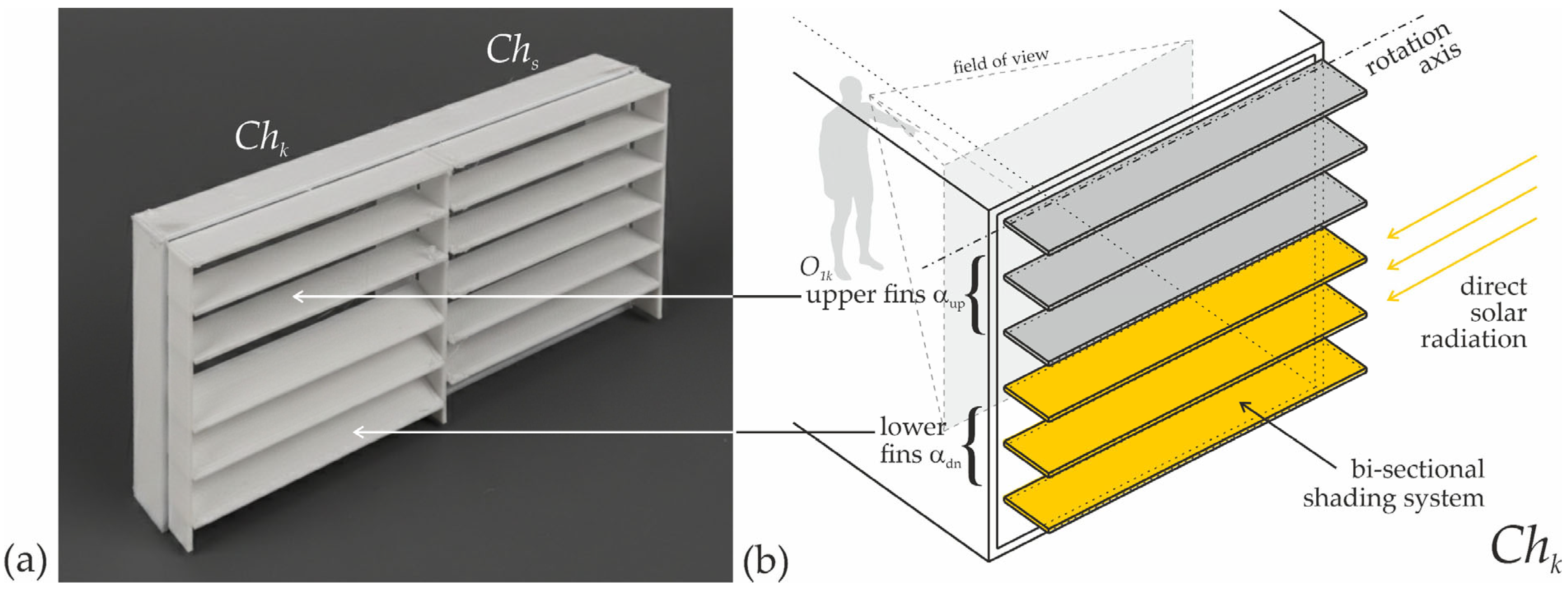
The experimental investigation was conducted using a reduced-scale physical mock-up (1:20); the reference test room in the simulation framework was designed to replicate the mock-up geometry. The mock-up comprises two adjacent chambers: a kinetic chamber (Ch_k), equipped with a working prototype of the bi-sectional KSS, and a static chamber (Ch_s), serving as a reference space with a shading system of identical dimensions but static (meaning: with the fin inclination angle = 0). The experimental setup is based on a testbed previously developed and tested by the author; a detailed technical description of the original configuration was provided in the Supplementary Materials of the earlier study [18]. No modifications to the physical configuration of the mock-up were introduced for the present investigation, except the installation of a static horizontal shading system in chamber Ch_s. Experimental façade testbeds under real sky conditions were also constructed by Andersen and Guillemin, which further supports the validity of the applied experimental method [29].

3.1.1. Materials and Equipment

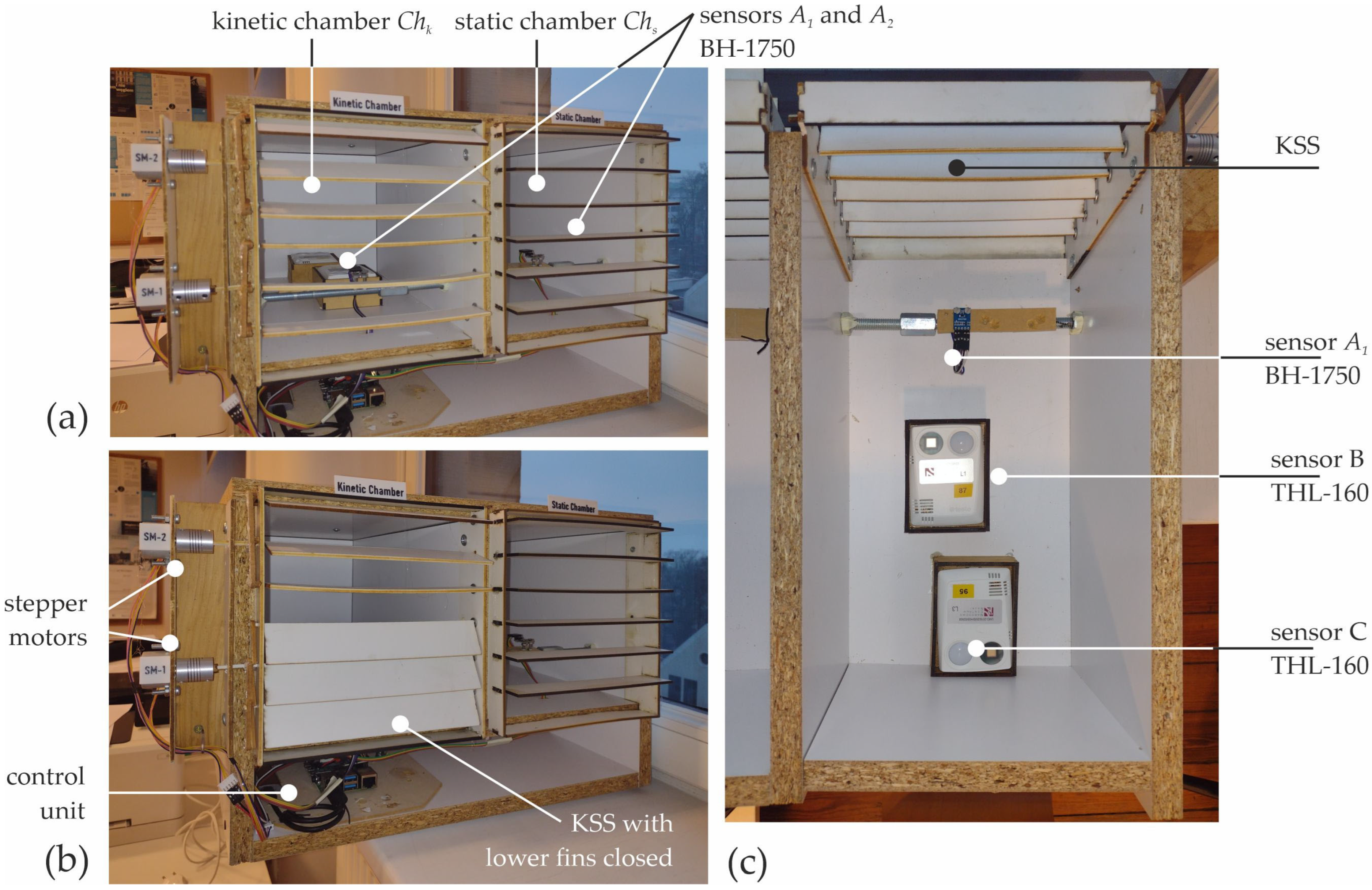
The reduced-scale mock-up was constructed at 1:20 scale (the geometry of the simulated reference test room precisely corresponds to that of the mock-up). The mock-up comprises two chambers: Ch_k, equipped with a prototype of the bi-sectional KSS, and Ch_s, serving as a reference configuration (Figure 1, Figure 2 and Figure 3).

3.1.2. Shading System Geometry

The test chambers had plan dimensions of 4 × 8 m and a height of 4 m; accordingly, the reduced-scale physical mock-up (1:20) measured 0.20 × 0.40 m and 0.20 m in height. The glazed opening in the front façade had dimensions of 0.20 × 0.20 m at model scale. Both chambers, the kinetic chamber (Ch_k) and the static reference chamber (Ch_s), were equipped with geometrically identical horizontal shading system composed of six parallel louvres with a depth of 0.63 m in full scale (32.5 mm at 1:20 scale). The shading prototype was fabricated from 3 mm laser-cut foamed PVC panels and mechanically coupled into two independently controlled groups of horizontal fins. Actuation was provided by two 5 V stepper motors M₁ and M₂ controlled via a Raspberry Pi 3 microcomputer. These shading elements are hereafter referred to as fins, as their depth significantly exceeds that of conventional louvres. In the kinetic chamber (Ch_k), the shading system was dynamically actuated by two stepper motors operating according to the control algorithm described in Section 3.1.6.

3.1.3. Sensors

Daylight measurements were recorded using two BH-1750 illuminance sensors (manufacturer ROHM Semiconductors Co., Ltd., Kyoto, Japan) installed inside the mock-up, with sensor A₁ located in Ch_k at a position corresponding to the virtual sensor used in simulations and the second A₂ placed in Ch_s [30]. An SSD unit was used for continuous data storage during the measurement campaign. Additionally, two TESTO THL-160 data loggers (manufact Testo SE & Co. KGaA, Titisee-Neustadt, Germany) were installed inside mock-up Ch_k to measure the illuminance in the middle of the room (hereafter referred to as physical sensor ‘B’) and in the back of the room (hereafter referred to as physical sensor ‘C’). Sensors B and C were used for detailed illuminance analysis in the study reported in [22]. Although they were physically integrated into the experimental mock-up, their data were not used in the glare analysis presented in the present study. The list of measuring equipment is presented in

Table 2. The list of measuring equipment.

No.	Device	Function	Items	Characteristics	Accuracy
1	BH-1750 FVI	daylight sensor	2	illuminance range 1–65,535 [lux]	±2 1 (±20)%
2.	Testo THL 160	daylight data logger	2	illuminance range 0–20,000 [lux]	±3% according to DIN 5032-7 Class L
				UV Radiation range 0–10,000 mW × m−2	±5%
3.	Kipp and Zonen CM 11	pyranometer	1	irradiance range 0–1400 W × m−2, sensitivity 4 to 6 [µV/W × m−2]	±3%

¹—minimal value (typical value), as stated by Rohm Semiconductors [30].

.

• Preliminary Studies, Pilot Study. Prior to the main measurement campaign, the mock-up was constructed in early May 2024 and subjected to a six-week pilot study conducted at a different location. During this period, the control software, data storage system, and log file structure were iteratively refined and tested under varying weather conditions to ensure stable operation and reliable data acquisition.

3.1.4. Variables, Data Curation

• Variables: The experimental framework defines the inclination angles of the upper and lower shading fins (α_up and α_dn) as independent variables, while indoor daylight illuminance E_h constitutes the dependent variable. The static geometric and material parameters of the mock-up were treated as control variables.
• Data Collection Methods. Illuminance values measured in Ch_k (E_hk) and Ch_s (E_hs), together with the corresponding fin inclination angles, were continuously recorded in a log file stored on an SSD drive with a temporal resolution of 2 s. In accordance with the postulate formulated by Carlucci et al. [31], the automated control algorithm enabled smooth and continuous fin rotation within an angular range of 0° to 60°, allowing for gradual system response rather than discrete positional steps.
• Data Analysis Plan The recorded log files were directly imported into spreadsheet software for further processing. Data normalisation was not required; instead, the preprocessing stage involved temporal downsampling to reduce data volume and to smooth short-term fluctuations in illuminance values. The analysis comprised descriptive statistics, including summary tables and graphical representations, followed by a comparative assessment between Ch_k, equipped with the bi-sectional KSS, and Ch_s, serving as the reference configuration. This comparison focused on quantifying the influence of fin inclination angles on indoor daylight illuminance, with particular attention given to the dynamic interaction between the upper and lower fin groups.
• Data Validity and Interpretation. For system control, the target indoor illuminance in C_hk was set to 3000 lx, consistent with the reference value used in the corresponding simulation study. A hysteresis band of ±300 lx was implemented to ensure stable system operation, allowing illuminance to vary between 2700 and 3300 lx. This control strategy reduced the frequency of fin adjustments and prevented oscillatory behaviour of the bi-sectional KSS under short-term fluctuations in daylight conditions.

The relatively high target indoor illuminance of 3000 lx at the façade-proximal sensor location (1.5 m) results from the depth of the analysed space (8 m) and the strong daylight attenuation observed with increasing distance from the façade in side-lit rooms. Previous measurements performed in the same experimental facility demonstrated that achieving acceptable daylight levels on the horizontal work plane in the rear part of the room (approximately 6–8 m from the façade) requires substantially higher illuminance values near the façade [22].

3.1.5. Installation, Orientation and Timeframe

• Installation. The mock-up was installed indoors behind a large glazed window within the faculty building. In this configuration, the existing window glazing effectively acted as an external glazing layer for the mock-up, reproducing the solar radiation accumulation typically associated with a fully glazed façade. This setup ensured realistic light transmission conditions while providing a controlled indoor environment. Additionally, indoor installation protected the mock-up and associated wiring from direct exposure to external weather conditions, thereby enhancing operational stability throughout the measurement campaign.
  Between the outdoor environment and the experimental chambers, solar radiation passes through the building window before reaching the mock-up. Although this may slightly affect the absolute magnitude of transmitted radiation due to the glazing’s transmittance and reflectivity, its influence on the comparative analysis between the two chambers is negligible, since both chambers were exposed to the same boundary conditions. The building window therefore functioned as a constant part of the measurement setup rather than as an experimental variable. Because both chambers are exposed to identical optical conditions, the glazing does not affect the comparative evaluation between the kinetic and static configurations.
• Orientation, timeframe. The mock-up was installed on a façade oriented 15° west of south, following the existing building geometry. As a result, the recorded dataset predominantly represents conditions between 13:00 and 18:00, corresponding to the period of highest solar irradiance. The 15° westward deviation is clearly reflected in the collected data, where the illuminance peak is shifted towards the afternoon hours. This time window, during which the mock-up was fully exposed to direct sunlight, defines the valid temporal scope of the experimental data and should be taken into account when interpreting the results.

3.1.6. Façade Closure Scheme, Control Logic

The KSS operates using two independently controlled groups of horizontal fins: an upper set (α_up) and a lower set (α_dn). This bi-sectional configuration allows different daylight control functions to be performed simultaneously.

• Control Parameters: The lower fins primarily regulate direct solar penetration and are responsible for limiting high-luminance sources that may generate glare near the façade, and at the workplane level of 0.85 m above the floor. The upper fins control the admission and redistribution of diffuse daylight deeper into the room. During operation, the system adjusts the fin angles based on the illuminance measured near the façade, maintaining the target range of 2700–3300 lx.

The following configurations and control logics have been applied in the system:

• Open Configuration: When the illuminance at sensor ‘A₁’ is below 3000 lx, both the upper and lower groups of façade fins remain in the open position, perpendicular to the façade (angle α_dn = 0° relative to the façade’s normal), denoted as the KSS configuration ‘open’.
• Down-Closed Configuration: When the illuminance at sensor ‘A₁’ exceeds the 3300 lx threshold (3000 lx threshold + 300 lx hysteresis), the lower fins automatically rotate to reduce the illuminance levels at sensor ‘A₁’. Lower fins rotate in 1° increments until the angle reaches 60°.
• All-Closed Configuration: When the illuminance level at sensor ‘A₁’ continues to exceed 3300 lx even after the lower fins have been adjusted, the upper fins are rotated to decrease the illuminance further. In the experiment, the upper fins rotate in 1° increments until the angle α_up reaches 60°.

This control logic represents an extended implementation of the simulation-based control scheme, informed by control strategies reported in earlier studies [22], which compared a kinetic chamber with a void chamber (no shading system). All changes in system configuration were driven by real-time data from illuminance sensor A₁ located in Ch_k and executed via stepper motors, thereby enabling a continuous and adaptive system response.

• Theoretical rationale. The separation of the façade into two independently controlled fin zones reflects the different daylight functions occurring within the visual field. The lower fins primarily regulate direct solar penetration and limit high-luminance sources that may generate glare near the façade. The upper fins control the admission and redistribution of diffuse daylight deeper into the room. The maximum and minimum rotation angles were defined to ensure both effective shading of direct solar rays and adequate daylight admission into the interior space. Complete closure of both fin groups was intentionally avoided, as such configurations produced daylighting conditions indicating the likely need for artificial lighting.
• System advantages. Compared with conventional single-zone automated blinds, the bi-sectional control strategy provides greater flexibility in balancing glare mitigation and daylight utilisation. By independently regulating direct solar penetration and diffuse daylight admission, the system can reduce glare from high-luminance sources while maintaining sufficient daylight levels deeper in the room.
• Accuracy and Randomisation. Measurement consistency was ensured by using the same type of daylight sensor (BH-1750) for all illuminance measurements, with sensor positions fixed throughout the campaign. Factory calibration was retained for all sensors. External solar irradiance conditions were monitored using data from the nearest meteorological station equipped with a CM11 pyranometer (Kipp and Zonen), located at the Meteorological Observatory of the Department of Climatology and Atmosphere Protection, Wrocław University (51°06′19.0″ N, 17°05′00.0″ E; elevation 116.3 m) [32].

3.1.7. Timing and Location

The measurement campaign was conducted over a one-month period, from 15 August to 20 September 2024. The analysed clear-sky days were selected within a period characterised by an extended window of predominantly clear-sky weather conditions. This unique weather-permitting window, spanning nearly two consecutive weeks, enabled the identification of three representative clear-sky days suitable for detailed glare analysis.

Within this period, variations in solar altitude and azimuth for corresponding hours were relatively small and can be considered negligible for the purposes of the present study. Consequently, the analysis does not aim to investigate seasonal variations in solar geometry but rather to assess the performance of the KSS under a consistent, well-defined set of clear-sky solar conditions. This constraint ensures that observed differences in glare metrics between the static (Ch_s) and kinetic (Ch_k) configurations are attributable primarily to system behaviour and control responses, rather than to changes in solar geometry.

The mock-up was located in Wrocław, Poland (51.11° N, 17.04° E). According to the Köppen climate classification, the local climate is classified as Cfb, bordering on Dfb when the 0 °C isotherm is applied. The experimental period corresponds to summer conditions characterised by high solar availability.

3.2. Hybrid Experimental–Simulation Method

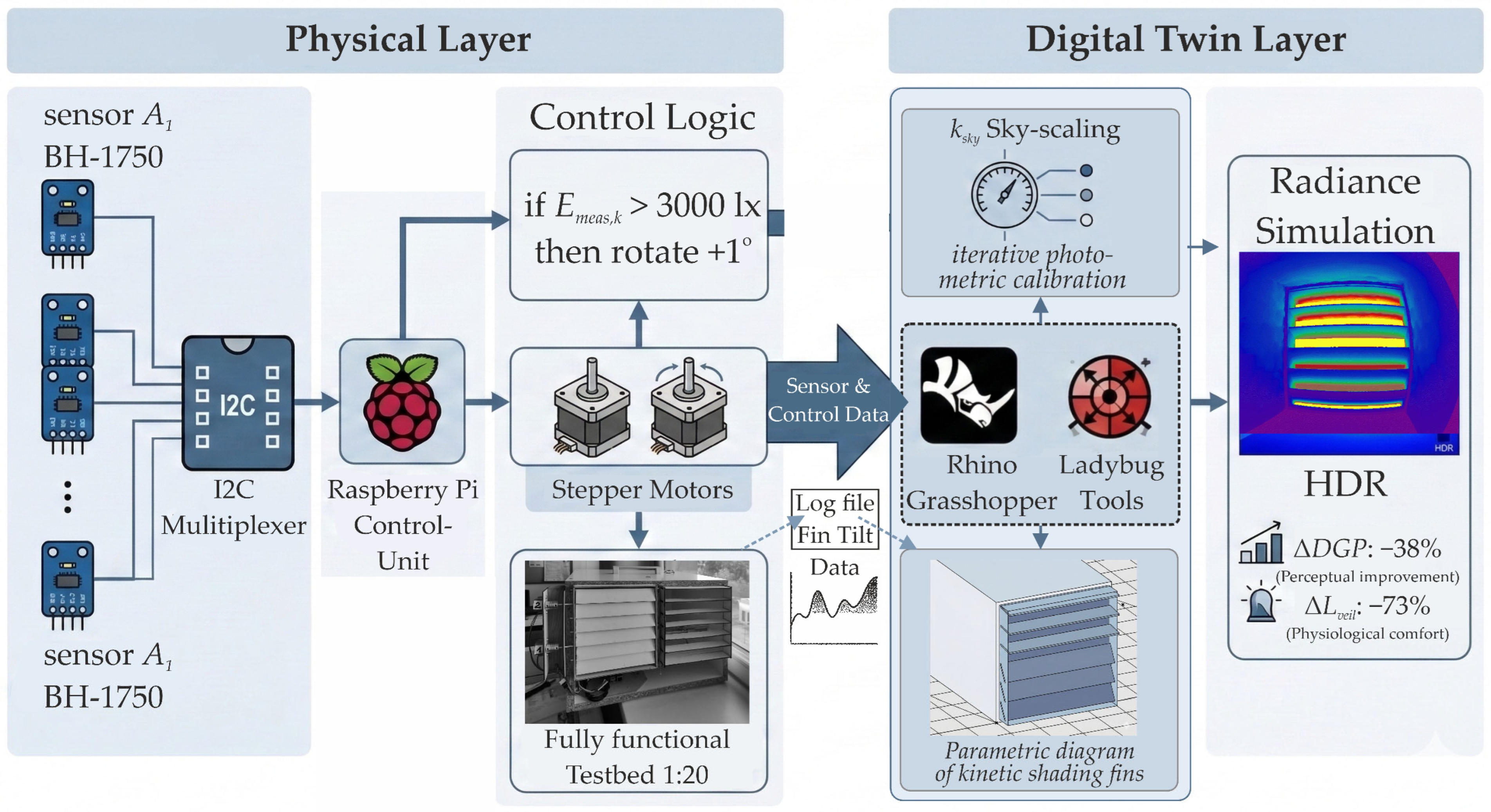
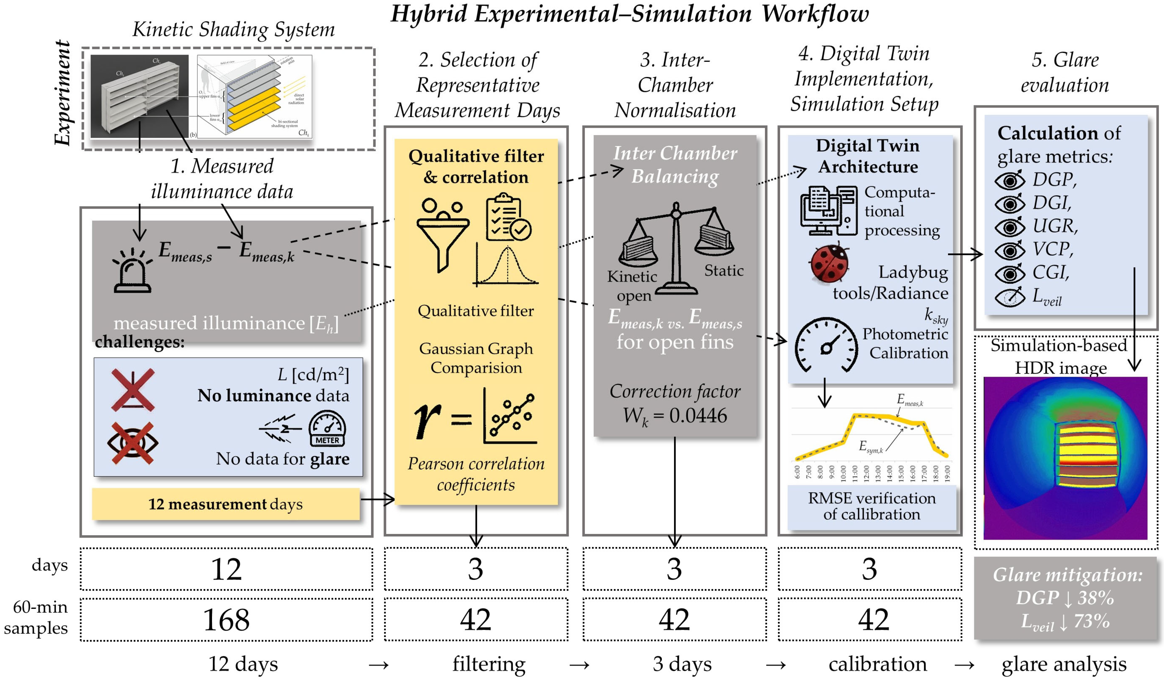
The performance of the KSS is evaluated using experimental data collected from a reduced-scale physical mock-up consisting of two test chambers: the kinetic chamber (Ch_k) and the static reference chamber (Ch_s), described in detail in the previous section. The analysis is conducted on a predefined subset of representative measurement days, selected according to the criteria outlined below. While the applied BH-1750 illuminance sensors provide reliable quantitative information on daylight availability (illuminance E_h), they do not enable direct assessment of glare-related visual comfort. To overcome this limitation, the study adopts an original calibrated experimental–simulation framework that integrates physical measurements with numerical daylight simulation within a single methodological workflow (see Figure 4).

3.2.1. Controlled Reproduction of the Sky

The core principle of the method is the controlled reproduction of the sky conditions observed during the experimental campaign within a simulation environment. A digital twin of the physical mock-up is implemented in the Radiance simulation framework using Grasshopper and Ladybug Tools (version 1.9.0). Climate-based sky models generated using the “HB Wea From Clear Sky” and “HB Climatebased Sky” components are calibrated so that the simulated illuminance values (E_sim) closely match the experimentally measured illuminance in the kinetic and static chambers (E_meas,k and E_meas,s, respectively).

The factor k_sky uniformly scales the simulated sky radiance distribution to reproduce the photometric conditions of the real sky, affecting the physical mock-up during the corresponding measurement interval (Figure 4). Its sole purpose is to bring E_sim,x and E_meas,x into amplitude agreement, without altering the relative luminance distribution of the sky. The sky-scaling factor k_sky was adjusted using successive approximations until the root mean square error (RMSE) between the measured illuminance profiles and the simulated values reached a minimum. This procedure allowed the simulated sky luminance distribution to accurately reproduce the photometric conditions observed during the experimental campaign, which is essential for the reliable evaluation of glare metrics derived from HDR luminance maps.

It should be noted that the applied sky-scaling procedure modifies only the overall radiometric amplitude of the sky luminance distribution and does not alter its angular structure. Consequently, potential modelling inaccuracies related to specific components of the “Perez sky” luminance distribution remain unchanged. These include, for example, the circumsolar brightening region around the solar disc, large-scale luminance gradients across the sky dome (e.g., zenith–horizon or north–south gradients), and atmospheric scattering effects associated with haze or veil luminance conditions [33]. The Perez all-weather sky luminance model was subsequently corrected in an erratum published by the original authors [33]. The implementation of the Perez sky model in Radiance follows the corrected formulation and includes parameterised representations of circumsolar brightening and large-scale sky luminance gradients derived from empirical sky measurements.

Consequently, the proportional relation between the direct (solar/circumsolar) and diffuse components of the Perez sky model remains preserved during the calibration procedure. Therefore, the sky-scaling factor k_sky serves solely as a photometric calibration parameter, ensuring consistency between simulated and measured indoor illuminance levels while preserving the physically based luminance distribution defined by the underlying sky model.

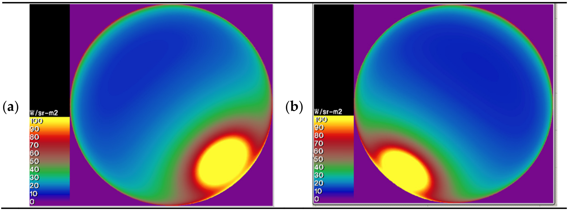
In the present implementation, this photometric scaling was achieved by adjusting the “clear-sky” parameter within the Ladybug/Radiance framework, as originally performed by Threlkeld and Jordan [34]. The resulting photometric effect is formally represented in this study by the sky-scaling factor k_sky, which describes the effective amplitude correction applied to the simulated sky luminance distribution. The applied scaling adjustments remained within a narrow range (approximately 0.95–1.20), indicating that only minor calibration corrections were required. The calibrated sky luminance distributions provided the boundary conditions for subsequent glare simulations, combined with the Perez sky luminance distribution model as implemented in Radiance (see Figure 5).

The quality of the calibration was assessed by minimising the discrepancy between measured and simulated illuminance time series under identical geometric and material boundary conditions. Calibration accuracy was quantified using statistical error metrics, primarily the root mean square error (RMSE). The calibration process was considered satisfactory when the relative root mean square error (RMSE_rel) between simulated and measured illuminance values remained below 15%, a threshold commonly adopted in daylight simulation validation studies. In the present study, RMSE_rel values ranged between 5.5% and 12.8%, indicating good agreement between simulated and measured illuminance.

High dynamic range (HDR) images are subsequently rendered in Ladybug for predefined viewpoints corresponding to the observer O_1k and O_1s position in the physical mock-up. Visual comfort is evaluated using the Daylight Glare Probability (DGP) metric calculated with the “evalglare tool” developed by Wienold and Christoffersen [35], executed via the Radiance-based workflow implemented in Grasshopper. This tool allows the calculation of glare-related indices, including Daylight Glare Probability (DGP), Daylight Glare Index (DGI), and veiling luminance (L_veil). In this way, the proposed framework extends the experimental analysis beyond illuminance-based metrics to luminance-based metrics, including glare perception under experimentally reproduced daylight conditions.

A sensitivity analysis was conducted by varying the assumed surface reflectance values by ±0.05 to quantify the influence of material uncertainty on glare prediction. The analysis confirmed that these variations did not affect the comparative performance trends observed between the static and kinetic shading configurations.

3.2.2. Selection of Representative Measurement Days

During the measurement campaign, external irradiance data from the meteorological station were unavailable due to a temporary pyranometer (CM11) malfunction. Consequently, direct reference measurements of global solar irradiance could not be used for the identification of clear-sky conditions. To address this limitation, the indoor illuminance measured in the static reference chamber (Ch_s) was used as a proxy indicator reflecting the temporal evolution of daylight conditions. Because the chamber geometry and glazing configuration remained unchanged throughout the campaign, variations in the recorded indoor illuminance closely followed changes in external daylight availability.

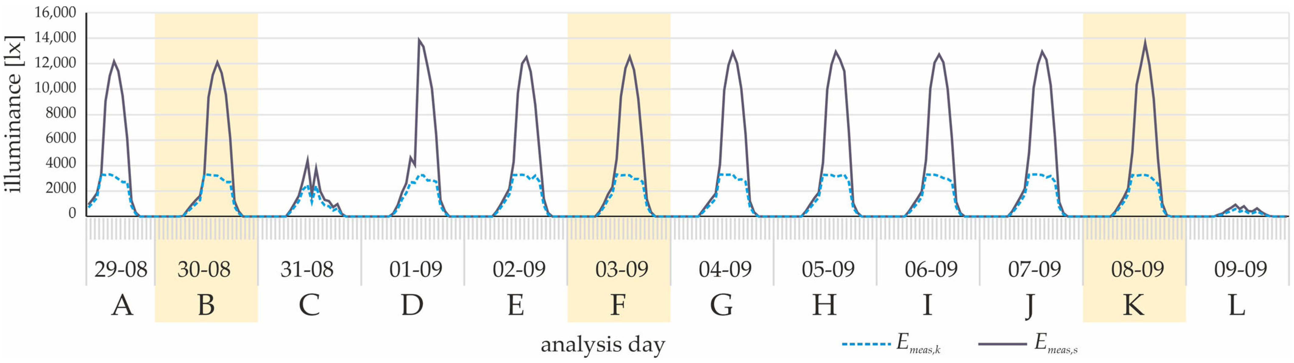
To ensure that the evaluation of the KSS was based on representative and statistically consistent data, a subset of measurement days was therefore selected from the full experimental dataset originally spanning from the 29th of August to the 9th of September, labelled “A” through “L”.

These days represented a range of sky conditions, including clear-sky, overcast (“L”), and partly cloudy (“C”) conditions, in order to capture the system’s response under different daylight scenarios. The illuminance E_meas,k and E_meas,s values collected in Ch_k and Ch_s are plotted on Figure 3. A preliminary analysis of the measured illuminance data indicated that days characterised by overcast “L” or mixed sky conditions “C” provided limited insight into the operational behaviour of the KSS. Under such conditions, the shading fins remained fully open in both the kinetic (Ch_k) and static (Ch_s) chambers; α_up and α_dn = 0. As a result, these cases did not warrant detailed simulation-based glare analysis and were treated only as reference or control conditions.

To identify the days characterised by the highest and most stable solar exposure among all remaining measurement days, the similarity between measured daylight profiles and an idealised reference curve was evaluated. For this purpose, a Gaussian reference curve was generated individually for each day and used as a “comparative template” rather than a physical model of solar radiation. Day “A”—29th of August featured only fragmentary data, therefore was skipped in the following analysis. Although not intended as a physical model of solar radiation, the Gaussian curve provides a convenient statistical approximation of the smooth bell-shaped diurnal irradiance pattern typically observed under clear-sky conditions, resulting from the gradual change in solar altitude during the day. This procedure conceptually follows the general principle used in clear-sky detection methods in solar radiation studies, where smooth diurnal irradiance curves are used as indicators of stable atmospheric conditions [36,37,38] (Figure 6).

The underlying assumption was that the measured illuminance E_meas,s in the chamber Ch_s, equipped with the static shading system, provides a consistent proxy reflecting variations in global daylight availability, thereby allowing the identification of days characterised by intense, temporally stable sunlight. For each day, the number of Gaussian values was matched exactly to the number of available daylight measurement points, corresponding to the 14 sunlight hours. This ensured that the comparison was conducted using aligned time intervals, without interpolation or resampling of the data. The Gaussian reference curve was defined as:

$$y(x)=e^{{-a(x-0.5)}^2}$$

(1)

The identification of clear-sky days was supported by a quantitative selection criterion based on the correlation between measured mock-up internal illuminance profiles and a theoretical Gaussian curve representing the expected diurnal pattern of solar irradiance under stable clear-sky conditions.

In Equation (1), the variable x represents a normalised daytime index ranging from 0 to 1 within the analysed time interval, where x = 0.5 corresponds approximately to the time of maximum solar elevation. The Gaussian function does not represent a physical model of daylight distribution. Instead, it serves as an idealised reference profile used to identify measurement days characterised by stable clear-sky conditions. Days whose measured illuminance curves showed the highest correlation with this smooth reference profile were considered representative clear-sky cases.

The Pearson correlation coefficient (r) and the associated p-value were used to quantify the similarity between the measured and theoretical illuminance curves. Days were ranked by r_Gauss after excluding cases with non-significant correlations (p-value ≥ 10⁻⁵). All reported correlations were statistically significant (p-value < 10⁻⁵), see

Table 3. Pearson correlation coefficients (r_Gauss) and associated p-values quantifying the similarity between measured illuminance profiles in the static chamber (Ch_s) and the corresponding Gaussian reference curves for individual measurement days. The p-values are reported in units of ×10⁻⁶. Days exhibiting the highest correlation coefficients were selected as representative clear-sky cases for subsequent analysis.

calendar day	30-08	01-09	02-09	03-09	04-09	05-09	06-09	07-09	08-09
day label	B	D	E	F	G	H	I	J	K
rGauss	0.9239	0.8241	0.9024	0.9471	0.8758	0.8664	0.8864	0.8921	0.9088
p-value (×10−6)	86.47	14.23	8.77	48.11	3.41	1.74	1.10	1.02	0.08

. The three days exhibiting the highest correlation coefficients with statistically significant p-values were classified as representative clear-sky days: “B”, “F”, and “K”. This procedure enabled exclusion of days affected by transient cloud cover or atmospheric instability, thereby ensuring consistent photometric conditions for subsequent sky calibration and glare analysis.

Consequently, the core analysis was restricted to three representative clear-sky days (“B”, “F”, “K”), corresponding to a total of 42 h of measurement data. This selection enabled assessment of the KSS under direct solar exposure, where adaptive fin movement in Ch_k is most relevant. The inclusion of multiple clear-sky days ensured that the analysis was not limited to a single solar geometry, but instead reflected system performance across a range of solar altitudes and azimuths throughout the day.

3.2.3. Influence of Sky-Scaling Calibration on Glare Metrics

To assess the impact of the proposed sky-scaling calibration on glare prediction, a comparative analysis of calibrated and uncalibrated simulations was conducted for selected representative cases where the sky-scaling factor differed most notably from unity for the static chamber Ch_s. When k_sky ≈ 1, calibrated and uncalibrated simulations are expected to generate only marginally different glare predictions.

The comparison shows that photometric calibration of the sky luminance distribution systematically increases predicted glare metrics, see

Table 4. Influence of sky-scaling calibration on glare metrics for selected representative cases in static chamber Ch_s. Uncalibrated (k_sky = 1) and calibrated simulations are compared.

Day	Hour	ksky	DGP (uncal.)	DGP (cal.)	ΔDGP	Lveil (uncal.)	Lveil (cal.)	ΔLveil
30 Aug.	11:00	1.2	0.38	0.41	0.034	609.47	726.84	117.37
30 Aug.	12:00	1.2	0.50	0.56	0.061	717.23	844.49	127.26
3 Sept.	11:00	1.2	0.39	0.42	0.034	638.10	755.51	117.41
3 Sept.	12:00	1.15	0.53	0.58	0.050	757.34	921.30	163.96
9 Sept.	11:00	1.2	0.39	0.42	0.034	633.34	753.71	120.37
9 Sept.	12:00	1.2	0.54	0.61	0.069	820.64	1118.92	298.28

. Across the analysed cases, DGP increased by approximately 0.03–0.07, indicating that uncalibrated simulations may underestimate glare under real sky conditions. The relative increase of DGP ranged from approximately 2% to 9%, while L_veil increased by up to about 18% after calibration. The comparison indicates that uncalibrated simulations tend to underestimate glare metrics. On average, the calibrated workflow increased DGP by 9.21% and veiling luminance by 17.86%, confirming that photometric calibration significantly affects glare prediction. This demonstrates the importance of performing photometric calibration, as it not only aligns illuminance levels but also ensures consistency between the glare metrics derived from the simulations.

A detailed comparison between calibrated and uncalibrated simulations is provided in the Supplementary Material (Table S1), where paired glare metrics are reported for each analysed day and hour together with the resulting relative differences.

3.2.4. Simulation Settings and Numerical Accuracy

Radiance employs a Monte Carlo–based ray-tracing algorithm; therefore, minor numerical variations may occur between simulation runs even when identical input parameters are used. These stochastic differences are typically limited to within ±2% for illuminance-related outputs. To minimise random variation and ensure numerical convergence, all simulations were performed using high-accuracy Radiance settings. The adopted parameters included an ambient bounce value of −ab 3, ambient divisions −ad 4096, ambient super-samples −as 1024, ambient accuracy −aa 0.1, and ambient resolution −ar 64 [39].

These settings were selected to ensure stable convergence of calculated illuminance values and consistency across all simulation runs conducted for both the kinetic and static chambers. By maintaining identical numerical settings throughout the analysis, the influence of stochastic variability inherent to Monte Carlo ray tracing was minimised, ensuring that observed differences in illuminance and glare metrics could be attributed to shading system behaviour rather than numerical artefacts.

4. Results

4.1. Inter-Chamber Normalisation, Raw Experimental Data Processing

The experimental testbed was designed such that the two measurement chambers—kinetic (Ch_k) and static (Ch_s)—were geometrically equivalent. In both chambers, the BH-1750 illuminance sensors A₁ and A₂ were installed at identical positions. When the shading fins were set to 0°, the shading systems Ch_k and static Ch_s were geometrically comparable and functionally identical. Under this configuration, the measured illuminance values in Ch_k and Ch_s would be expected to coincide.

In practice, minor discrepancies between the two datasets of E_meas,k and E_meas,s were observed. These differences can be attributed to small geometric deviations introduced during manual assembly of the reduced-scale mock-up, despite all shading components being laser-cut from a common CAD model, as well as to slight variations in the photometric response of the BH-1750 sensors. To account for these effects, an inter-chamber photometric normalisation was applied. Using measurement periods under overcast conditions, without direct solar radiation and with fully open fins (α_up and α_dn = 0°), a correction factor of W_k = 0.0446 (4.46%) was determined as the median relative difference between illuminance measured in the kinetic chamber (E_meas,k) and the static chamber (E_meas,s). All illuminance values measured in Ch_s were subsequently rescaled by a factor of 0.9554 (1 − W_k) to align both datasets to a common reference level defined by Ch_k.

Following normalisation, the similarity between the two illuminance series E_meas,k and E_meas,s was quantified using multiple statistical metrics. A Pearson correlation coefficient of r_norm = 0.9858 indicates a very strong linear relationship between the datasets. The mean absolute error (MAE_norm) was 62.56 lx, while the root mean square error (RMSE_norm) reached 115.79 lx, both reflecting relatively small deviations between corresponding values. The coefficient of determination (R² = 0.9607), obtained from linear regression, indicates that approximately 96.0% of the variance in one dataset is explained by the other. Together, these results confirm a high level of agreement between the normalised datasets, supporting their suitability for comparative quantitative analysis.

Relative Illuminance Reduction Achieved by the KSS

To quantify the effectiveness of the KSS in reducing indoor illuminance, the analysis focused on periods when the system was actively operating, defined as non-zero fin inclination angles (α_up ≠ 0° and/or α_dn ≠ 0°). For each hour of active operation, the ratio between illuminance measured in the static chamber and that measured in the kinetic chamber was calculated as:

$$R_h={\displaystyle \frac{E_{meas,s}}{E_{meas,k}}}$$

The hourly ratios were subsequently averaged over the analysed period. The resulting mean ratio was $\overline{R}$ = 2.21, indicating that the illuminance level in the kinetic chamber was, on average, approximately 1/$\overline{R}$ ≈ 0.45 of that recorded in the static chamber during the same hours. This corresponds to a mean illuminance reduction of approximately 55% on average achieved by the KSS relative to the static configuration under direct solar exposure.

4.2. Simulation-Based Glare Evaluation Results

The comparison of horizontal illuminance levels recorded in the static (Ch_s) and kinetic (Ch_k) chambers demonstrates a substantial reduction in indoor illuminance achieved by the KSS. However, horizontal illuminance alone is insufficient to fully characterise visual comfort, particularly under conditions of direct solar exposure. For this reason, the experimental results were complemented by simulation-based analyses to quantify glare-related visual comfort metrics in both chambers.

The assessment of glare in the adjacent static (Ch_s) and kinetic (Ch_k) chambers was conducted in the following steps:

• Digital twin. A simulation model of the experimental setup was created and implemented in Rhino using the Grasshopper parametric platform. The simulation model reproduced the geometry of the reduced-scale mock-up. Virtual observers were positioned at the centre of each chamber (O_1k and O_1s) and “looking” towards the glazed façade, reproducing typical viewing conditions during daylight exposure.
• Sky calibration. To reproduce the daylight conditions observed during the experimental campaign, a single simulated sky model was employed and photometrically calibrated against experimentally measured indoor illuminance data, in accordance with the assumptions defined in Section 3.2.1. The calibration was performed independently for each analysed hour to match simulated illuminance values to the corresponding measurements in the kinetic (Ch_k) and static (Ch_s) chambers.
• Verification of the sky calibration procedure. Once the simulated illuminance (E_sim,k) in the reference configuration corresponded to the measured illuminance (E_meas,k) in the kinetic chamber Ch_k, the sky model was considered calibrated for that specific time step. For this verification, E_meas,k, E_meas,s, and the corresponding E_sim,k and E_sim,s values were plotted against each other, and statistical validation metrics, such as RMSE, were calculated [40].
• Glare-related metrics were calculated for two virtual observer positions, O_1k in the kinetic chamber and O_1s in the static chamber, both located at the centre of the respective spaces and oriented towards the glazed façade. By adapting the photometric scaling of the sky luminance distribution to the measured indoor illuminance levels for each analysed condition, for each observer position, high dynamic range (HDR) images were generated and subsequently analysed to calculate glare-related indices, including Daylight Glare Probability (DGP), Daylight Glare Index (DGI), and veiling luminance (L_veil). As the kinetic mechanism is primarily activated under clear-sky conditions, the core analysis focuses on three representative clear-sky days (“B”, “F”, and “K”), corresponding to sunny conditions. In total, glare simulations were conducted for 42 individual hourly cases. This approach enabled the evaluation of the KSS under particularly critical conditions characterised by direct solar exposure. This simulation setup enabled a direct, condition-consistent comparison of glare indices between the static and kinetic configurations, forming the basis for the quantitative results presented in Section 4.2.3.

This combined evaluation framework enables a direct comparison between the static and kinetic configurations that extends beyond illuminance-based metrics. While the measured illuminance values quantify the overall amount of light entering the space, the glare indices capture the spatial distribution of luminance and the presence of high-luminance regions within the observer’s field of view. As a result, the analysis provides a comprehensive assessment of visual comfort, identifying conditions under which the KSS reduces glare relative to the static configuration, as well as situations in which adaptive fin movement modifies the perceptual characteristics of the visual environment.

4.2.1. Verification of Calibration

Table 5. Statistical validation metrics comparing measured E_meas,k, E_meas,s and simulated illuminance E_sim values in the static (Ch_s) and kinetic (Ch_k) chambers for three representative clear-sky days.

	Analysis Day:	30 AUG		3 SEP		8 SEP
Stat. Metrics	State:	Static	Kinetic	Static	Kinetic	Static	Kinetic
RMSEabs	Absolute Root Mean Square error	187.6	236.2	273.5	143.6	224.1 (429.9) *	186.1
RMSErel	Relative Root Mean Square Error	0.055	0.128	0.076	0.075	0.118	0.100
NRMSErange	Normalised Root Mean range-normalised)	0.022	0.072	0.031	0.044	0.045	0.057
MdAPE	Median Absolute Percentage Error	0.052	0.069	0.012	0.076	0.040	0.080

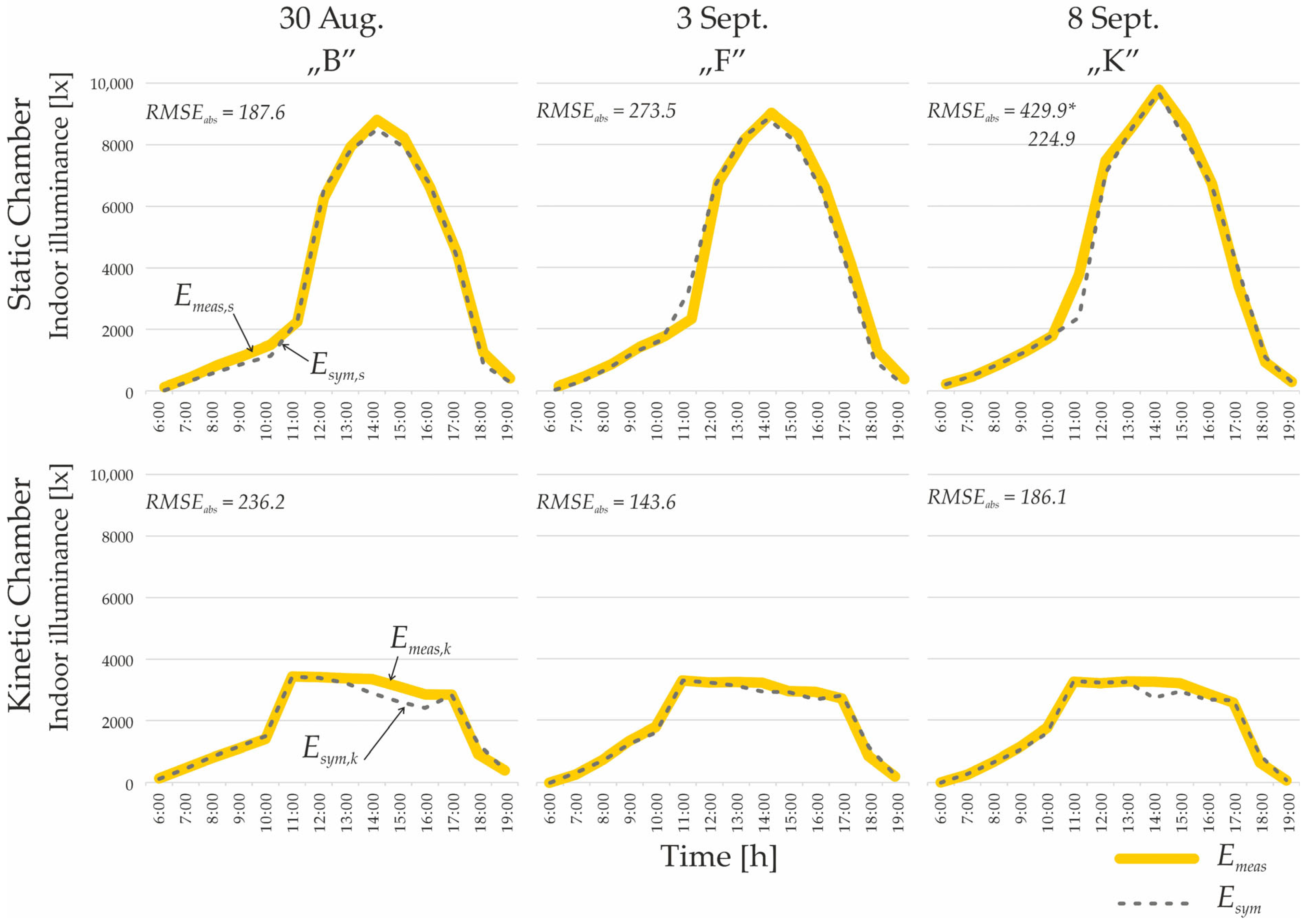
* Values in parentheses indicate RMSE_abs before removal of the outlier.

summarises the statistical validation metrics comparing measured and simulated illuminance values (E_meas and E_sim) for the static (Ch_s) and kinetic (Ch_k) chambers across three representative clear-sky days (30 August, 3 September, and 8 September). The measured interior illuminance under clear-sky conditions aligns with expected profiles described in classical daylight coefficient methods [41], providing confidence in the experimental setup. The results indicate a high level of agreement between experimental measurements and simulation outputs.

For the static chamber, the absolute RMSE values ranged from 187.6 lx to 273.5 lx, while for the Ch_k they remained between 143.6 lx and 236.2 lx. Relative error metrics were consistently low, with RMSE_rel values between 0.055 and 0.128 and normalised RMSE (NRMSE_range) not exceeding 0.072 (7.2%), remaining below commonly adopted reference threshold 10% threshold for photometric model validation. Median Absolute Percentage Error (MdAPE) values were similarly low, typically ranging from 0.012 to 0.080, confirming stable correspondence between measured and simulated illuminance.

A deviation was observed in the static configuration on 8 September, with a single data point recorded around 11:00 resulting in a pronounced increase in RMSE. This outlier was associated with direct solar incidence on the sensor during the simulation, yielding an illuminance of approximately 45,000 lx. After excluding this data point from the analysis, the RMSE for that day decreased from 430 lx to 224 lx, restoring consistency with the remaining validation results (see Figure 7).

Although the calibration procedure is based on agreement between measured and simulated indoor illuminance values, this approach provides a physical constraint on the underlying luminance distribution. In glare analysis, the relevant quantity is the vertical illuminance at the observer’s eye (E_v), which represents the hemispherical integral of luminance over the visible sky hemisphere and can be expressed as:

$$E_v=\underset{\Omega }{\int }L\left(\theta , \phi \right) cos\theta d\omega$$

where L(θ,φ) is the luminance distribution across the sky dome, θ is the angle between the incident light direction and the normal to the vertical plane at the observer’s eye, Ω represents the hemisphere of directions contributing to the vertical illuminance, and dω is the differential solid angle.

When a physically based sky model (Perez sky) is used, matching simulated and measured illuminance effectively constrains the hemispherically integrated luminance distribution within the observer’s field of view. Under these calibrated conditions, the HDR luminance maps generated by Radiance provide photometrically consistent estimates of the daylight environment, and can therefore be used to compute glare indices such as DGP, DGI, and L_veil.

Although the control algorithm of the KSS is based on horizontal illuminance measured near the façade by sensor A₁, this parameter remains strongly correlated with the luminance distribution within the observer’s field of view, i.e., the spatial distribution of daylight entering the space. Consequently, maintaining façade-proximal illuminance within a controlled range indirectly limits excessive luminance values within the field of view and contributes to reducing glare metrics such as DGP and L_veil.

Overall, the statistical comparison confirms the robustness of the calibrated simulation framework across the analysed clear-sky conditions. The validated simulation results are therefore used in the subsequent analysis as input for calculating Daylight Glare Probability (DGP) and related glare metrics, enabling a reliable comparative assessment of visual comfort performance between the static and kinetic façade systems.

4.2.2. Primary and Supplementary Glare Evaluation Metrics Used in This Study

Visual comfort was evaluated using three glare-related metrics: Daylight Glare Probability (DGP), Daylight Glare Index (DGI), and veiling luminance (L_veil). These indices were selected to provide complementary perceptual and physiological perspectives on glare under dynamic daylight conditions and to ensure consistency with both contemporary and earlier daylighting research.

• Daylight Glare Probability (DGP) is the primary metric used in this study. It quantifies the probability of discomfort glare perceived by an observer based on the luminance distribution within the visual field, explicitly accounting for vertical eye illuminance and the presence of high-luminance sources. DGP values below 0.35 correspond to imperceptible glare, values between 0.35 and 0.40 indicate perceptible but acceptable glare, and values exceeding 0.40 are generally associated with disturbing glare. Due to its robustness under daylight conditions and its widespread adoption in recent research, DGP serves as the main indicator of perceptual glare in the present analysis.
• Daylight Glare Index (DGI) is included as a complementary metric to facilitate comparison with earlier daylighting studies. Although DGI has been largely superseded by DGP in contemporary research, it remains relevant for benchmarking results against legacy datasets and historical literature. DGI is expressed on a logarithmic scale, with values above approximately 24 commonly interpreted as indicating intolerable glare.
• Veiling luminance (L_veil) represents the physiological component of glare associated with intraocular light scattering in the human eye, occurring primarily in the cornea, crystalline lens, and vitreous body. Unlike perceptual glare indices, L_veil directly quantifies the luminance veil superimposed on the retinal image, which reduces visual contrast and acuity. Lower L_veil values indicate clearer retinal images and improved visual conditions, providing an objective physiological complement to perceptual glare metrics such as DGP and DGI. L_veil is expressed in candela per square metre (cd/m²).

In addition to the primary glare metrics discussed in detail in this study (DGP, DGI, and L_veil), several supplementary indices commonly reported in the literature—namely UGR, VCP, and CGI—were also calculated. These indices are reported in tabular form to provide a broader context and to confirm the consistency of glare-related trends between the static and kinetic configurations. However, because they do not provide interpretive value beyond the selected primary metrics under dynamic daylight conditions, they are not discussed further in the main text.

4.2.3. Glare Results for Static and Kinetic Systems

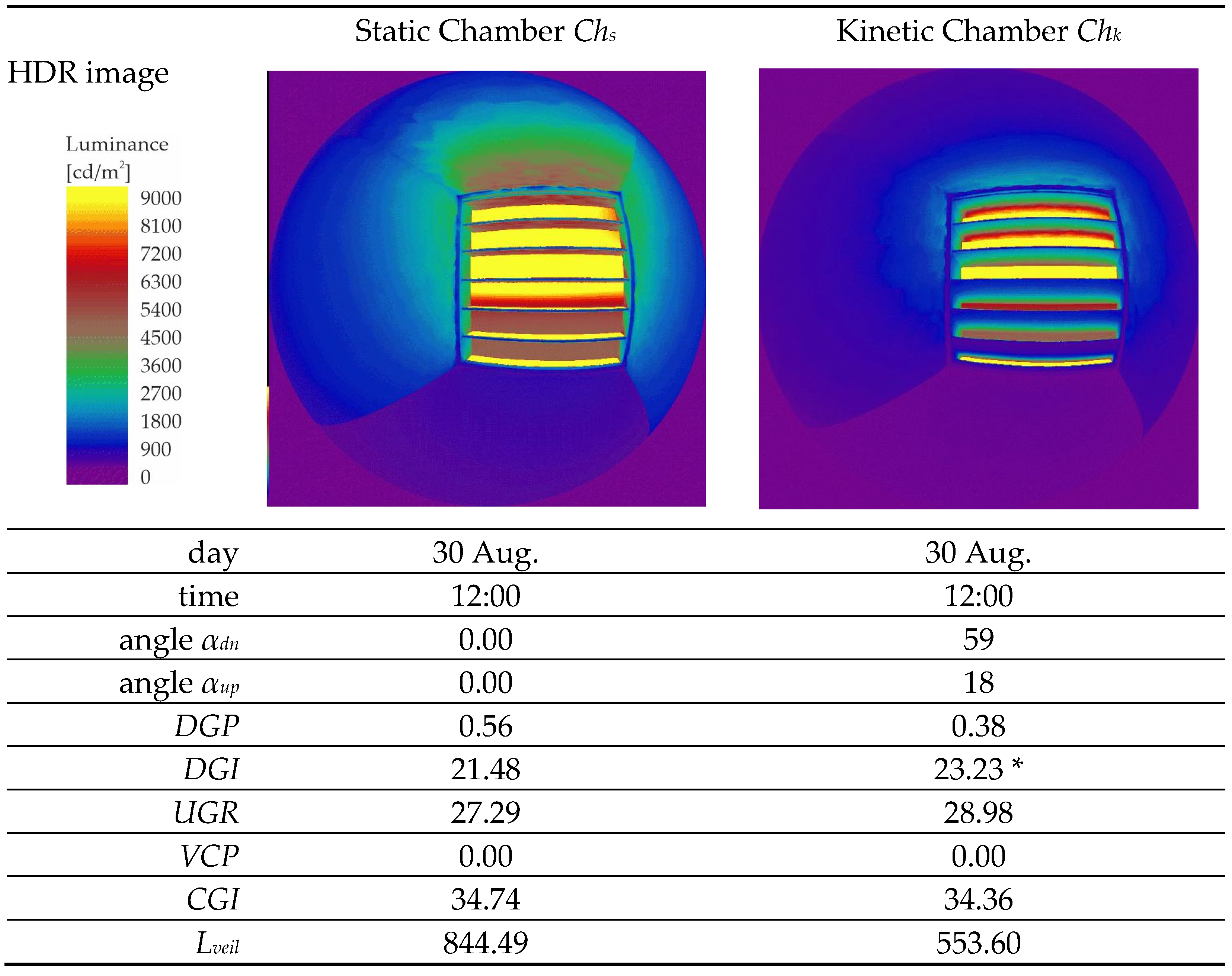
The glare analysis focused on three representative clear-sky days—30 August, 3 September, and 8 September—and compared two façade configurations: a static horizontal shading system and a kinetic system with adaptively controlled fins. The evaluation was restricted to the period between 11:00 and 17:00, corresponding to the hours of highest direct solar exposure. During this interval, glare was most pronounced, and the KSS mechanism was active, enabling a meaningful comparison of glare-related performance between the KSS and static configurations. Figure 8 shows simulated HDR luminance images and complementary glare metrics for a single time step at 12:00 on the “B” day.

Table 6. Combined analysis (30 August–8 September), average results (hours 11:00–17:00).

Index	Chs (Mean)	Chk (Mean)	Absolute Difference	Δ [%]	Interpretation
DGP	0.57	0.35	0.22	−38%	Reduction of DGP from 0.57 to 0.35 (−38%), shifts glare conditions from the “disturbing glare” range toward the threshold of “perceptible glare”.
DGPmax	0.72	0.36	0.36	−50%	Peak glare is reduced by almost half during critical hours.
DGI	23.19	22.41	0.78	−3.4%	Slight improvement, consistent with DGP trend.
Lveil	1689 cd/m2	452 cd/m2	1237 cd/m2	−73%	Substantial reduction of veiling luminance.
UGR	29.04	27.60	1.44	−5%	Noticeable improvement within an acceptable range.
VCP	0.05	1.40	1.35	+2700%	Minor absolute change, but same positive trend.
CGI	35.97	32.70	3.27	−9%	Clear improvement; shift below discomfort threshold.

presents the combined analysis of glare metrics. All glare metrics for all days and hours are provided in Supplementary Table S2.

It is worth noting that, while the KSS significantly reduces the overall probability of glare (DGP), a marginal increase in the contrast-based DGI is observed at 12:00; this suggests that, although vertical eye illuminance is lowered, the specific adaptive fin angles may introduce localised luminance contrasts to which the DGI is particularly sensitive.

5. Discussion

Interpretation of Glare Reduction Results

While the present analysis focuses on a narrow late-summer clear-sky window defined by the available measurement conditions, the applied calibration-based workflow is readily transferable to other seasons, enabling future investigations of kinetic shading performance under a broader range of solar geometries.

Across the analysed clear-sky days, the most pronounced differences in glare performance between the KSS and static configurations occurred around 14:00, corresponding to the period of strongest direct solar exposure and highest luminance contrast within the test chambers. The inclusion of peak glare values (DGP_max) confirms the consistency of this pattern. In the static chamber (Ch_s), DGP_max values reached 0.70, 0.71, and 0.75 on the respective analysed days, indicating extremely disturbing glare conditions. Under identical external conditions, the KSS reduced DGP to approximately 0.35–0.36, corresponding to perceptible but acceptable glare levels. Although glare was not fully eliminated, the reduction of DGP from approximately 0.70–0.75 to 0.35–0.36 demonstrates the strong mitigation potential of adaptive fin movement.

When averaged across all analysed days, the kinetic façade consistently outperformed the static configuration in terms of visual comfort. Mean DGP values decreased from 0.57 to 0.35, representing an average reduction of approximately 38% during peak solar exposure. At the same time, veiling luminance (L_veil) was reduced from 1689 cd/m² to 452 cd/m², corresponding to a 73% decrease in retinal light scatter and masking luminance. This pronounced reduction in L_veil provides physiological support for the perceptual improvements indicated by DGP.

Complementary glare indices, including DGI, UGR, and CGI, exhibited consistent downward trends, supporting the robustness of the observed results across different evaluation frameworks. Although absolute VCP values remained low under daylighting conditions, their relative increase further corroborates the overall tendency toward improved subjective comfort in the kinetic configuration.

Overall, the KSS demonstrated a stable, reproducible ability to reduce both perceptual and physiological glare across days and varying sky conditions. The adaptive motion of the 0.63 m-deep fins proved particularly effective during the critical period between 11:00 and 17:00, when direct solar radiation poses the highest glare risk. These findings indicate that kinetic shading not only improves average visual comfort but also suppresses extreme glare during peak sunlight exposure, which is particularly relevant for daylight-dominated interior spaces.

Beyond the absolute magnitude of glare reduction, the presented results demonstrate the value of combining calibrated experimental measurements with simulation-based glare evaluation. In contrast to purely simulation-driven studies, the proposed workflow enables glare metrics to be assessed under photometrically validated sky conditions, reducing uncertainty associated with uncalibrated sky models. This methodological aspect is particularly relevant for the evaluation of KSS operating under highly variable daylight conditions.

6. Conclusions

This study presented a calibrated experimental–simulation framework for evaluating glare reduction achieved by a horizontal KSS under real daylight conditions. By combining reduced-scale physical measurements with photometrically calibrated sky simulations, the approach enabled photometrically validated glare assessment using both perceptual (DGP, DGI) and physiological (L_veil) metrics. The results demonstrate that adaptive fin movement substantially reduces both average and peak glare under clear-sky conditions, particularly during periods of direct solar exposure. Beyond the specific case study, the proposed workflow provides a transferable methodology for the evaluation of adaptive façade systems under variable sky conditions, supporting more reliable visual comfort assessments in daylight-driven architectural design.

Future studies may extend the presented workflow to different seasonal conditions, façade orientations, and adaptive control strategies; however, these aspects lie beyond the scope of the present investigation.

Limitations of the Study

The experimental investigation was conducted using a reduced-scale physical mock-up, an approach previously demonstrated to be suitable for daylight evaluation in architectural research [42,43,44]. While the reduced-scale experimental setup provides a cost-effective and highly controlled environment for evaluating KSS geometries, it is important to acknowledge the inherent limitations of physical scaling. Specifically, the challenge of precisely replicating the specular and diffuse reflectance properties of full-scale architectural materials at a reduced scale may introduce minor photometric discrepancies. Furthermore, while the digital twin effectively calibrates the sky luminance parameters, future studies at a 1:1 scale would be beneficial to fully validate the system’s performance regarding complex inter-reflections and real-world mechanical tolerances

The experimental configuration, while ensuring high data stability and repeatability through indoor placement, inherently isolated the mock-up from dynamic outdoor environmental stressors such as wind loads and precipitation. Furthermore, the measurement campaign was limited to a specific late-summer window under clear-sky conditions, therefore excluding seasonal variations in solar geometry and performance under overcast or intermediate skies.

While these constraints delineate the specific boundary conditions of the current study, the results validate the core control logic and visual comfort assessment methods, establishing a robust methodological baseline for future long-term evaluations of KSS across diverse climatic contexts.

References

1. UNEP; Global Alliance for Buildings and Construction (GlobalABC). Global Status Report for Buildings and Construction 2024/2025: Not on Track to Net Zero; United Nations Environment Programme: Nairobi, Kenya, 2024; Available online: https://globalabc.org/sites/default/files/2025-03/Global-Status-Report-2024_2025.pdf (accessed on 23 January 2026).
2. Ürge-Vorsatz, D.; Khosla, R.; Bernhardt, R.; Chan, Y.C.; Vérez, D.; Hu, S.; Cabeza, L.F. Heating and cooling energy trends and drivers in buildings. Renew. Sustain. Energy Rev. 2020, 129, 109911. [Google Scholar] [CrossRef]
3. Chau, C.K.; Hui, W.K.; Ng, W.Y.; Powell, G.W. Overview of embodied energy in building materials and energy-saving potential. Energy Build. 2015, 86, 251–259. [Google Scholar]
4. Tzempelikos, A.; Shen, H. Comparative control strategies for roller shades with daylighting and energy considerations. Build. Environ. 2013, 67, 30–44. [Google Scholar] [CrossRef]
5. ASHRAE. ASHRAE Handbook—Fundamentals; American Society of Heating, Refrigerating and Air-Conditioning Engineers: Atlanta, GA, USA, 2021; Chapter 18. [Google Scholar]
6. Peel, M.C.; Finlayson, B.L.; McMahon, T.A. Updated world map of the Köppen–Geiger climate classification. Hydrol. Earth Syst. Sci. 2007, 11, 1633–1644. [Google Scholar] [CrossRef]
7. Tzempelikos, A.; Athienitis, A.K. The impact of shading design and control on building cooling and lighting demand. Sol. Energy 2007, 81, 369–382. [Google Scholar] [CrossRef]
8. O’Brien, W.; Gunay, H.B. The contextual factors contributing to occupants’ adaptive comfort behaviors in offices—A review and proposed modeling framework. Build. Environ. 2014, 77, 77–87. [Google Scholar] [CrossRef]
9. Boyce, P.R. Human Factors in Lighting, 3rd ed.; CRC Press: Boca Raton, FL, USA, 2014. [Google Scholar]
10. Reinhart, C.F.; Walkenhorst, O. Validation of dynamic RADIANCE-based daylight simulations for a test office with external blinds. Energy Build. 2001, 33, 683–697. [Google Scholar] [CrossRef]
11. Attia, S.; Bilir, S.; Safy, T.; Struck, C.; Loonen, R.; Goia, F. Current Trends and Future Challenges in the Performance Assessment of Adaptive Façade Systems. Energy Build. 2018, 179, 165–182. [Google Scholar] [CrossRef]
12. Tabadkani, A.; Roetzel, A.; Li, H.X.; Tsangrassoulis, A. A Review of Automatic Control Strategies Based on Simulations for Adaptive Facades. Build. Environ. 2020, 175, 106801. [Google Scholar] [CrossRef]
13. Loonen, R.C.G.M.; Rico-Martinez, J.M.; Favoino, F.; Brzezicki, M.; Menezes, C.; La Ferla, G.; Aelenei, L. Design for Façade Adaptability: Towards a Unified and Systematic Characterization. Energy Procedia 2015, 78, 1284–1289. [Google Scholar]
14. Loonen, R.C.G.M.; Trčka, M.; Cóstola, D.; Hensen, J.L.M. Climate adaptive building shells: State-of-the-art and future challenges. Renew. Sustain. Energy Rev. 2013, 25, 483–493. [Google Scholar] [CrossRef]
15. Attia, S.; Lioure, R.; Declaude, Q. Future trends and main concepts of adaptive facade systems. Energy Sci. Eng. 2020, 1, 3255–3272. [Google Scholar] [CrossRef]
16. COST Action TU1403—Adaptive Facades Network. Available online: https://tu1403.eu/ (accessed on 24 January 2026).
17. Luna-Navarro, A.; Loonen, R.; Juaristi, M.; Monge-Barrio, A.; Attia, S.; Overend, M. Occupant-Facade interaction: A review and classification scheme. Build. Environ. 2020, V177, 106880. [Google Scholar] [CrossRef]
18. Brzezicki, M. A Systematic Review of the Most Recent Concepts in Kinetic Shading Systems with a Focus on Biomimetics: A Motion/Deformation Analysis. Sustainability 2024, 16, 5697. [Google Scholar] [CrossRef]
19. Yunitsyna, A.; Sulaj, E. Daylight Optimization of the South-Faced Architecture Classrooms Using Biomimicry-Based Kinetic Facade Shading System. J. Daylighting 2025, 12, 1–20. [Google Scholar] [CrossRef]
20. Hosseini, S.M.; Mohammadi, M.; Guerra-Santin, O. Interactive Kinetic Façade: Improving Visual Comfort Based on Dynamic Daylight and Occupant’s Positions by 2D and 3D Shape Changes. Build. Environ. 2019, 165, 106396. [Google Scholar] [CrossRef]
21. Martinho, H.; Loonen, R.; Hensen, J.L.M. Evaluating the Impact of High-Resolution Irradiation Data on the Daylight Performance Assessment of Adaptive Solar Shading Systems. Build. Environ. 2024, 262, 111816. [Google Scholar] [CrossRef]
22. Brzezicki, M. Enhancing Daylight Comfort with Climate-Responsive Kinetic Shading: A Simulation and Experimental Study of a Horizontal Fin System. Sustainability 2024, 16, 8156. [Google Scholar] [CrossRef]
23. Gaber, B.; Zhan, C.; Han, X.; Omar, M.; Li, G. Enhancing Daylight and Energy Efficiency in Hot Climate Regions with a Perforated Shading System Using a Hybrid Approach Considering Different Case Studies. Buildings 2025, 15, 988. [Google Scholar] [CrossRef]
24. Xiong, J.; Chan, Y.; Tzempelikos, T. Model-Based Shading and Lighting Controls Considering Visual Comfort and Energy Use. In Proceedings of International Conference CISBAT 2015 Future Buildings and Districts Sustainability from Nano to Urban Scale; LESO-PB, EPFL: Lausanne, Switzerland, 2016; pp. 253–258. [Google Scholar] [CrossRef]
25. Kurniasih, S.; Musdinar, I.; Rachmanto, B. Daylight Intensity of Reading Room with Shading Device’s Opening (Case Study: The Library of Universitas Budi Luhur, South Jakarta). In Proceedings of the EduARCHsia & Senvar 2019 International Conference (EduARCHsia 2019); Atlantis Press: Dordrecht, The Netherlands, 2020. [Google Scholar] [CrossRef]
26. Fikery, A.A.; Hamed, R.E.; Ali, N.A. Improve Lighting Balance Performance and Energy Consumption by Using Kinetic Adaptive Skin for Office Space in Cairo, Egypt. Civ. Eng. Archit. 2024, 12, 135. [Google Scholar] [CrossRef]
27. Hao, W.; Xu, J.; Zhao, F.; Sohn, D.-W.; Shi, X. Integration of Photovoltaic Shading Device and Vertical Farming on School Buildings to Improving Indoor Daylight, Thermal Comfort and Energy Performance in Three Different Cities in China. Buildings 2024, 14, 3502. [Google Scholar] [CrossRef]
28. Sorooshnia, E.; Rashidi, M.; Rahnamayiezekavat, P.; Rezaei, F.; Samali, B. Optimum External Shading System for Counterbalancing Glare Probability and Daylight Illuminance in Sydney’s Residential Buildings. Eng. Constr. Archit. Manag. 2021, 30, 296–320. [Google Scholar] [CrossRef]
29. Andersen, M.; Guillemin, A. A holistic approach to daylighting control: Comparison of various control strategies through a year of measurements. Sol. Energy 2005, 79, 159–170. [Google Scholar]
30. Rohm Semiconductors. Ambient Light Sensor IC Series. Digital 16bit Serial Output Type Ambient Light Sensor IC; Technical Note. BH-1750 FVI; Rohm Semiconductors: Kyoto, Japan, 2011; Available online: https://www.mouser.com/catalog/specsheets/Rohm_11162017_ROHMS34826-1.pdf (accessed on 1 June 2024).
31. Carlucci, F.; Loonen, R.C.G.M.; Fiorito, F.; Hensen, J.L.M. A Novel Approach to Account for Shape-Morphing and Kinetic Shading Systems in Building Energy Performance Simulations. J. Build. Perform. Simul. 2022, 16, 346–365. [Google Scholar] [CrossRef]
32. Markowicz, K.M.; Stachlewska, I.S.; Zawadzka-Manko, O.; Wang, D.; Kumala, W.; Chilinski, M.T.; Makuch, P.; Markuszewski, P.; Rozwadowska, A.K.; Petelski, T.; et al. A Decade of Poland-AOD Aerosol Research Network Observations. Atmosphere 2021, 12, 1583. [Google Scholar] [CrossRef]
33. Perez, R.; Seals, R.; Michalsky, J. All-weather model for sky luminance distribution—Preliminary configuration and validation. Sol. Energy 1993, 50, 235–245, Erratum in Sol. Energy 1993, 51, 423. https://doi.org/10.1016/0038-092x(93)90157-j. [Google Scholar] [CrossRef]
34. Threlkeld, J.L.; Jordan, R.C. Direct solar radiation available on clear days. ASHRAE Trans. 1958, 64, 45–56. [Google Scholar]
35. Wienold, J.; Christoffersen, J. Evaluation methods and development of a new glare prediction model for daylight environments with the use of CCD cameras. Energy Build. 2006, 38, 743–757. [Google Scholar] [CrossRef]
36. Reno, M.J.; Hansen, C.W. Identification of periods of clear sky irradiance in time series of GHI measurements. Renew. Energy 2016, 90, 520–531. [Google Scholar] [CrossRef]
37. Long, C.N.; Ackerman, T.P. Identification of clear skies from broadband pyranometer measurements and calculation of downwelling shortwave cloud effects. J. Geophys. Res. 2000, 105, 15609–15626. [Google Scholar] [CrossRef]
38. Ineichen, P.; Perez, R. A new airmass independent formulation for the Linke turbidity coefficient. Sol. Energy 2002, 73, 151–157. [Google Scholar] [CrossRef]
39. Kharvari, F. An empirical validation of daylighting tools: Assessing Radiance parameters and simulation settings in Ladybug and Honeybee against field measurements. Sol. Energy 2020, 207, 1021–1036. [Google Scholar] [CrossRef]
40. Zheng, D.; Chen, Y. Daylighting simulation and experimental validation of granular aerogel glazing system. In Proceedings of the 18th IBPSA Conference, Shanghai, China, 4–6 September 2023; pp. 3035–3041. [Google Scholar]
41. Tregenza, P.R.; Waters, I.M. Daylight coefficients for calculating interior illuminance. Light. Res. Technol. 1983, 15, 65–71. [Google Scholar]
42. Mandalaki, M.; Tsoutsos, T. Solar Shading Systems: Design, Performance, and Integrated Photovoltaics; Springer: Cham, Switzerland, 2019. [Google Scholar]
43. Bahdad, A.A.S.; Fadzil, S.F.S.; Taib, N. Optimisation of Daylight Performance Based on Controllable Light-shelf Parameters using Genetic Algorithms in the Tropical Climate of Malaysia. J. Daylighting 2020, 7, 122–136. [Google Scholar] [CrossRef]
44. Zazzini, P.; Romano, A.; Di Lorenzo, A.; Portaluri, V.; Di Crescenzo, V. Experimental Analysis of the Performance of Light Shelves in Different Geometrical Configurations Through the Scale Model Approach. J. Daylighting 2020, 7, 37–56. [Google Scholar] [CrossRef]
Figure 1. Preparatory design validation of the horizontal shading systems: (a) 3D-printed study model at a 1:80 scale representing the kinetic (Chk) and static (Chs) horizontal shading configurations, developed during the early design phase to verify geometric proportions, fin spacing, and system differentiation prior to fabrication of the reduced-scale (1:20) experimental mock-up; (b) conceptual schematic of the bi-sectional horizontal shading system showing the division into upper fins (αup) and lower fins (αdn), their common rotation axis, the observer field of view (FOV) and the observer O1k, and the direction of direct solar radiation. The schematic illustrates the functional logic of the kinetic configuration (Chk), in which both fin groups are independently adjustable.
Sustainability 18 03052 g001
Figure 2. Mock-up setup to collect measurements: (a) mock-up view with Chk and Chs; (b) mock-up view with KSS with lower fins closed, showing stepper motors and control unit; (c) top view of mock-up with removed top cover (ceiling) showing the BH-1750 sensor A1 and sensors B and C (THL-160) in the kinetic chamber Chk; the dash-dot line indicates the central axis of the chamber.
Sustainability 18 03052 g002
Figure 3. System architecture of the experimental–simulation framework linking the physical testbed and the digital twin environment. BH-1750 illuminance sensors connected to a Raspberry Pi control unit regulate stepper-motor-driven shading fins in the 1:20 façade mock-up. Measured data are transferred to a Rhino/Grasshopper–Ladybug model, where sky-scaling calibration ksky enables Radiance HDR simulations and glare assessment (DGP, Lveil).
Sustainability 18 03052 g003
Figure 4. Methodological workflow for glare analysis of the KSS, from measured horizontal illuminance data to simulation-based HDR image generation and glare evaluation. The procedure includes selecting representative clear-sky cases, inter-chamber photometric normalisation, and calibrated Radiance-based simulations. Glare metrics (DGP, DGI, UGR, VCP, CGI, and veiling luminance Lveil) were calculated for 42 hourly cases. The aggregated results indicate a 38% reduction in DGP and a 73% reduction in veiling luminance for the kinetic configuration relative to the static chamber.
Sustainability 18 03052 g004
Figure 5. Examples of calibrated climate-based sky radiance distributions used in the simulation framework for two representative measurement days (3 September at 15:00 and 9 September at 11:00) (a,b). Each sky dome represents the radiance distribution expressed in W/(m2·sr) after photometric calibration of the simulated sky, ensuring agreement with experimentally measured indoor illuminance. The colour scale is identical for all cases to allow direct comparison of sky luminance structure under different solar geometries. The maps exhibit a pronounced high-radiance region corresponding to the solar disc and its circumsolar area. Because the physical radiance of the solar disc is several orders of magnitude higher than that of the sky dome, radiance values within the solar disc are clipped to the upper limit of the colour scale (e.g., 100 W/(m2·sr)) to maintain visual readability.
Sustainability 18 03052 g005
Figure 6. Time series of Emeas in the kinetic (yellow) and static (blue) chambers over the analysed period (29-08 to 09-09). The plot illustrates the repeatability of clear-sky daily profiles used to select representative analysis days.
Sustainability 18 03052 g006
Figure 7. Comparison of measured and calibrated simulated indoor illuminance profiles for three representative clear-sky days (30 August, 3 September, and 8 September). Results are shown for the reference static chamber (Chs, top row) and the kinetic chamber (Chk, bottom row). Simulated sky conditions were calibrated hourly to match measured illuminance at the reference sensor point, thereby providing the basis for subsequent glare analysis. Measured illuminance profiles are shown with a thicker yellow line to improve visual readability and to clearly distinguish measured trends from the corresponding simulated curves. * The higher RMSE observed for the static chamber on 8 September reflects transient deviations around peak direct solar exposure.
Sustainability 18 03052 g007
Figure 8. Comparison of simulated HDR luminance images (identical luminance scale) and glare metrics for the static (Chs) and kinetic (Chk) chambers at 12:00 under clear-sky conditions. * DGI is particularly sensitive localised luminance contrasts.
Sustainability 18 03052 g008