Exploring the Multiscale Spatiotemporal Dynamics of Ecosystem Service Interactions and Their Driving Factors in the Taihu Lake Basin, China

Abstract

Understanding the intricate interrelationships among ecosystem services (ESs) is fundamental to advancing sustainable ecological management. This study focuses on the Taihu Basin and examines five representative ESs, including water yield (WY), carbon sequestration (CS), soil retention (SR), habitat quality (HQ), and crop production (CP), for the years 2000, 2010, and 2020. Spatial distribution characteristics and spatiotemporal dynamics were quantified through the combined application of the InVEST model, a food production model, and ArcGIS. Spearman correlation analysis and K-means clustering were then applied to characterize trade-offs and synergies among ESs and to delineate ecosystem service bundles at multiple spatial scales, including 1 km × 1 km grids, 10 km × 10 km grids, and the county level, while GeoDetector was used to identify the associated driving mechanisms. The results indicated that (1) between 2000 and 2020, the spatial distribution pattern of the ESs in the Taihu Basin underwent significant changes, with WY and SR increasing by 48.97% and 51.89%, respectively, while HQ, CS, and CP decreased by 17.2%, 15.5%, and 47.6%. (2) From an overall perspective of trade-offs and synergies, the interactions among ESs shifted from trade-offs (r < 0) to synergies (r > 0) as the scale increased. From the perspective of the spatial characteristics of trade-offs and synergies, the intensity of these interactions varied significantly with increasing scale, but the trend remained relatively stable. (3) The Taihu Basin can be categorized into six ES bundles (ESBs). ESB 1, ESB 3, ESB 4, and ESB 5 have relatively stable ES structures, whereas ESBs 2 and 6 display significant variations. (4) The primary factors influencing ESs vary significantly across different spatial scales, with land use/land cover (LULC) and the proportions of arable land, forestland, and buildings exhibiting strong explanatory power. This highlights the critical role of coupled natural and anthropogenic processes in shaping the spatial patterns of ESs. This study considers the spatiotemporal variation and scale dependence of ecosystem services, providing management recommendations tailored to different regions and spatial scales, and offering a scientific basis for regional ecological planning and watershed governance.

1. Introduction

Ecosystem services (ESs) are the environmental conditions and utilities provided by ecosystems that sustain human life and well-being [1,2,3]. Their stability and functionality are crucial for the sustainable development of society and the economy [4]. Currently, the degradation of ESs has garnered significant attention globally [5,6,7,8], making ecosystem assessment, management, and policy formulation essential [9]. The key to ecosystem management lies in understanding the interrelationships among ESs, which helps enhance their sustainable supply [10,11,12]. These interrelationships include trade-offs, synergies, and ES bundles (ESB) patterns [13,14]. Trade-offs occur when an increase in one ES comes at the expense of another, whereas synergies mean that multiple ESs increase or decrease simultaneously [15]. ESBs represent a set of multiple ESs that recur over time and space [16,17].

Scholars have developed various methods to evaluate ESs, such as the mass assessment method [18], value assessment method [19], energy value assessment method [20], and model assessment method [21,22,23,24]. The model assessment method, in which the interactions and impacts among various elements in ecosystems are considered, provides comprehensive and precise evaluation results, making it highly valuable for local decision-making. However, this method requires high-quality data. It is essential to explore the relationships between ESs on the basis of evaluations.

Common methods for investigating the trade-offs and synergistic relationships among ESs include Pearson or Spearman correlation analysis [25], partial correlation analysis [26], the mean square error (MSE) method [27], the Bayesian belief network [28], and geographically weighted regression (GWR) [29]. Pearson correlation analysis is frequently used but relies on strict assumptions of linearity and data normality. The partial correlation analysis method can eliminate the interference of irrelevant factors and more clearly reveal changes in trade-offs and synergy relationships in time series, but the selection of irrelevant factors is subjective. The MSE method can characterize non-uniform changes in ecosystem services in the same direction, yet it is not intuitive in expressing the positive and negative correlations (directionality) between ecosystem service relationships. The GWR method is commonly used to analyze trade-off and synergy relationships and their strength, and to quantify the spatial heterogeneity of factors affecting these relationships, but it is not suitable for data that may have multicollinearity. In contrast, Spearman correlation analysis, which does not require strict assumptions about data distribution, was employed to robustly capture potential nonlinear relationships among ESs. The resulting correlation coefficients directly indicate the strength and direction (positive or negative) of pairwise associations between ESs. This approach is widely used in studies of the trade-offs and synergistic relationships among ESs [29,30,31]. Research methods for identifying ESBs include K-means clustering [17], self-organizing map (SOM) network analysis [32], and principal component analysis (PCA) [33]. PCA is widely used for dimensionality reduction, but it assumes linear relationships among variables. Although SOM networks excel at handling non-linear data, they require a large amount of calculation for iterative convergence and involve complex hyperparameter tuning. Conversely, the Calinski–Harabasz (CH) criterion combined with K-means clustering offers advantages such as low computational complexity, strong interpretability, high adaptability and high robustness to data distributions, making it widely used in related research [34,35,36,37].

Research on ESs has evolved significantly from static, single-scale assessments to dynamic, multi-scale spatial analyses. Early studies were often confined to a single scale [38,39,40], which made it difficult to fully reveal the complex dynamics of ESs, potentially leading to decision-making biases [17,41]. Recognizing these limitations, recent studies have increasingly focused on the “scale effect,” where scholars have reported that the relationships among ESs and the corresponding influencing factors exhibit heterogeneity across different spatial scales [42,43,44]. For example, Hou et al. evaluated the trade-offs and synergies of multiple ESs in northern China’s mountainous regions and reported that synergies between food production and climate regulation were weak at the grid scale but strengthened significantly at the township and county scales [45]. Conversely, Chen et al. observed a divergent trend in the Yangtze River Delta, reporting that the synergy between water resource regulation and other ESs was stronger at the grid scale than at the county scale [46]. These studies suggest that relationships among ecosystem services are scale-dependent and represent a context-dependent process rather than a uniform rule. Zhou et al. further demonstrated that driving factors also exhibit scale effects. They reported that population density negatively impacts habitat quality at the 1 km scale, yet this effect becomes to a positive influence at the 10 km scale [47]. These studies indicated that the relationships among and driving factors of ESs vary significantly and display uncertainty across different spatial scales; Therefore, further multiscale research is required.

The Taihu Basin, an important ecological and economic region in eastern China, faces challenges related to water pollution, habitat degradation, and imbalance between the supply and demand of ESs due to urbanization, industrialization, and agricultural activities. Research has focused primarily on changes in ESs given policy impacts, such as ’returning farmland to lakes’, the impact of land use changes on ESs [48], and the assessment of interactions among ESs at a single scale [49]. Current research in the Taihu Basin has not fully elucidated the complex scale dependence among multiple ESs. Existing studies often treat spatial scales as isolated static units, failing to reveal spatial variations in the intensity of trade-offs and synergies or how the dominance of driving factors shifts across hierarchies. Consequently, systematic evidence regarding these scale conversion mechanisms and the spatiotemporal dynamics of ESBs remains insufficient, which limits the efficacy of ecological management and leads to policy recommendations that lack spatial targeting. To address these research gaps, this study selected the period from 2000 to 2020, a critical phase characterized by rapid urban expansion and intensive ecological engineering in the Taihu Basin. Taking advantage of the high availability of ecological and socio-economic data during this period, we conducted a multi-scale analysis based on 1 km grids, 10 km grids, and county-level units, aiming to provide targeted, scale-specific recommendations for regional ecological management. The specific research objectives are to (1) analyze the spatiotemporal distribution characteristics of ESs in the Taihu Basin, (2) explore the interrelationships among ESs at different scales, and (3) investigate the main driving factors affecting the ES supply at different scales. The findings support the optimization of regional ecological management in the Taihu Basin and the formulation of ecological protection policies, which are crucial for ensuring the ecological security of the lower Yangtze River and promoting the integrated development of the Yangtze River Delta.

2. Materials and Methods

2.1. Study Area

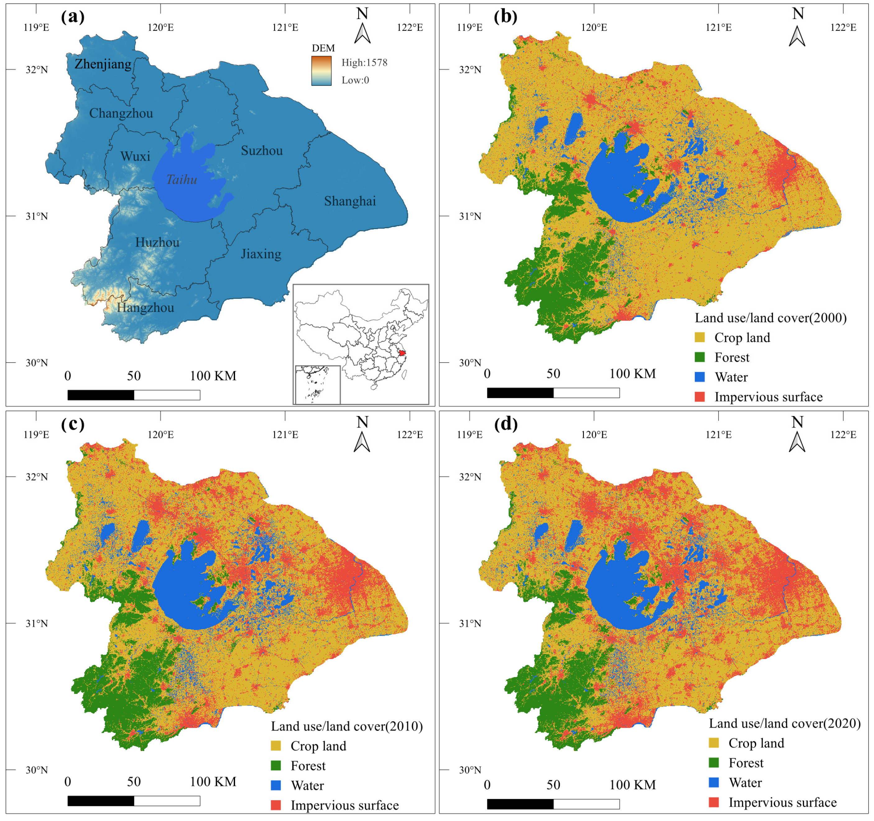
The Taihu Basin is situated in the eastern part of China, within the Yangtze River Delta (30° 28′–32° 15′ N, 119° 11′–121° 53′ E), covering an area of approximately 3.69 × 10⁴ km² (Figure 1). It encompasses Shanghai and parts of Jiangsu, Zhejiang, and Anhui Provinces. This basin is characterized by a subtropical monsoon climate, with an average annual temperature of 15–17 °C and average annual precipitation totaling 1000–1400 mm. The climate is humid, with distinct seasonal changes. The terrain within the basin is diverse, with the southwestern region consisting mainly of hills and mountains, whereas the northern and eastern areas are predominantly plains and water networks [50]. As a vital ecological barrier for the Yangtze River Delta, the Taihu Basin plays a crucial role in maintaining biodiversity, ensuring water resource security, and maintaining an ecological balance.

Additionally, the Taihu Basin is among the most economically developed regions in China, standing at the forefront of the country’s urban and industrial evolution. Statistical data from 2020 indicates a total population of 67.55 million, or 4.8% of the country, alongside a gross domestic product of 9.9978 trillion yuan, constituting 9.8% of the national GDP. The urbanization rate of 68.2% markedly surpassed the national average of 56.1% [51], fostering a highly compacted urban agglomeration characterized by vigorous economic performance. While the landscape is primarily dominated by arable land, forests, water bodies, and impervious surfaces, the footprint of developed urban terrain has expanded continuously in response to rapid modernization.

These spatiotemporal land cover dynamics, derived from the 30 m Annual Land Cover Dataset described in

Table 1. Summary of the Primary Data.

Data Name	Data Format	Data Source	Spatial Resolution
Temperature	Raster	National Earth System Science Data Center http://www.geodata.cn (accessed on 13 December 2024)	1 km
Precipitation	Raster	National Earth System Science Data Center http://www.geodata.cn (accessed on 13 December 2024)	1 km
Evapotranspiration	Raster	Loess Plateau Subcenter, http://loess.geodata.cn (accessed on 13 December 2024)	1 km
Soil Depth	Raster	Dataset by Shangguan et al. (2019), Scientific Data [53]	1 km
Soil Properties (Texture, Carbon)	Raster	Harmonized World Soil Database (HWSD) (v1.1) http://data.tpdc.ac.cn (accessed on 13 December 2024)	30 arc-second
DEM	Raster	Geospatial Data Cloud platform https://www.gscloud.cn(accessed on 13 December 2024)	30 m
Soil Type	Raster	Resource and Environment Science and Data Center http://www.resdc.cn (accessed on 13 December 2024)	1 km
NDVI	Raster	Long-term NDVI Dataset (1982–2020), Science Data Bank [54]	30 m
PM2.5	Raster	ChinaHighPM2.5(TPDC) https://www.tpdc.ac.cn (accessed on 13 December 2024)	1 km
LULC	Raster	China Land Cover Dataset (CLCD) by Yang and Huang [55]	30 m
Crop Production	Spreadsheet	Statistical Yearbooks (Zhejiang, Jiangsu, Anhui, Shanghai) http://tjj.zj.gov.cn/; https://tj.jiangsu.gov.cn/; http://tjj.ah.gov.cn/; https://tjj.sh.gov.cn (accessed on 13 December 2024)	County
Population Density	Raster	World Pop https://www.worldpop.org (accessed on 13 December 2024)	30 arc-second
GDP	Raster	Resource and Environment Science and Data Center http://www.resdc.cn (accessed on 13 December 2024)	1 km

, are illustrated in Figure 1b–d. Nevertheless, such precipitous growth has engendered critical environmental impediments, specifically aquatic eutrophication, atmospheric contamination, soil pollution, and intensifying urban heat island effects [52]. Although the government have deployed a spectrum of ecological restoration and governance measures that have yielded partial efficacy, including holistic watershed regulation, nonpoint source pollution mitigation, and wetland recovery, a discrepancy persists regarding national conservation targets. Consequently, more nuanced management strategies are requisite to ensure the sustained amelioration of the watershed’s ecological integrity.

2.2. Data Sources and Processing

In this study, various datasets, including digital elevation model (DEM), precipitation data, soil data (including soil depth [53]), crop production data (wheat, maize, and rice), long-term NDVI dataset [54], land use/land cover (LULC) data [55], and other relevant indicators, were used. All the raster data were resampled to a spatial resolution of 1 km by 1 km, and the coordinate systems for all the datasets were standardized to WGS_1984_UTM_Zone_50N. For more details on the data, see Table 1.

2.3. Research Methods

2.3.1. Ecosystem Service Assessment

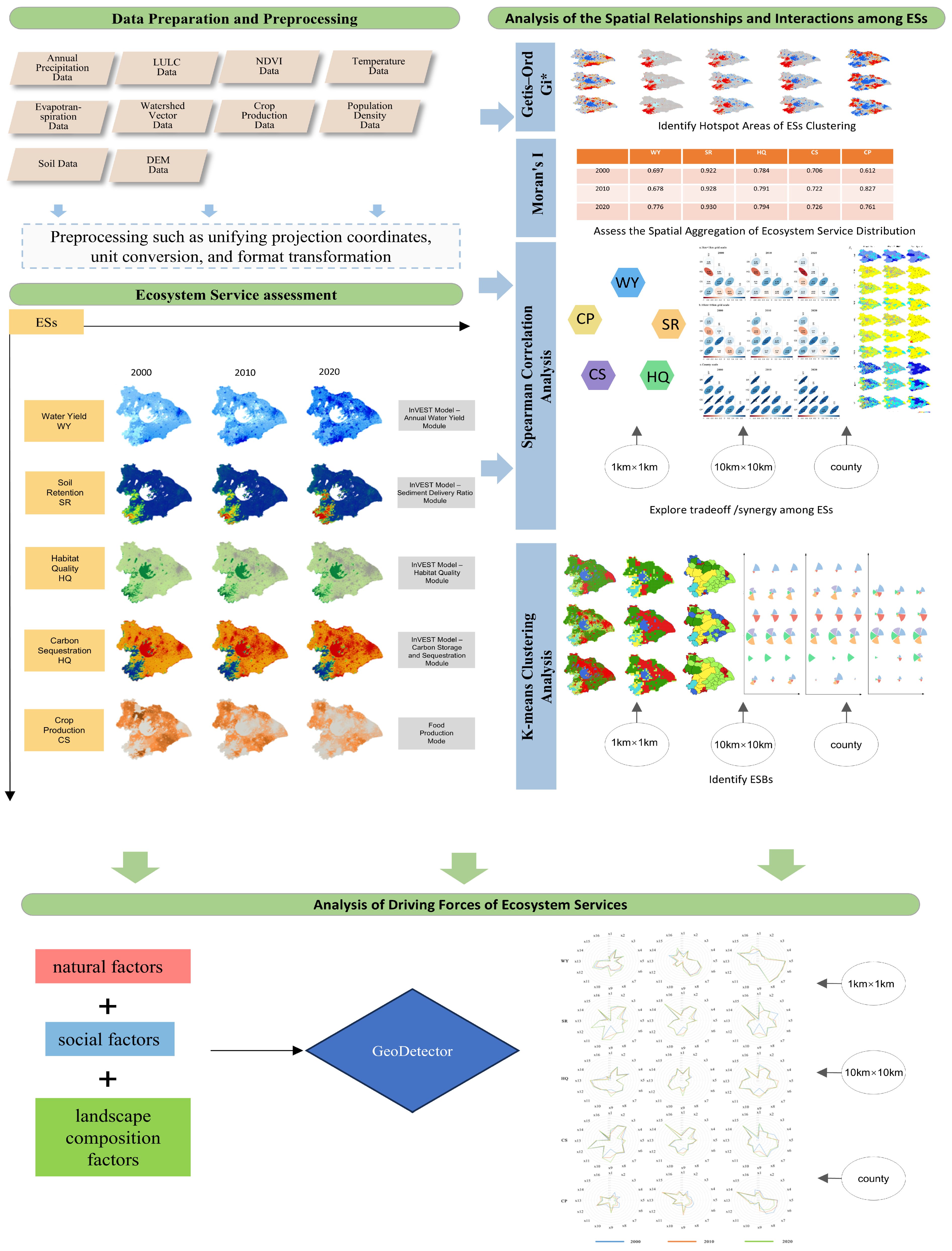
In this study, we identified five ESs to determine the fine-scale effects of ESs (Figure 2) on the basis of the following criteria: (1) representativeness of the ecological conditions in the study area, (2) alignment with ecological protection goals, and (3) availability and feasibility of data. First, using the InVEST model and food production model at a 30 m resolution [56], we quantitatively assessed the water yield (WY), soil retention (SR), carbon sequestration (CS), habitat quality (HQ), and crop product (CP) in the Taihu Basin for 2000, 2010, and 2020. This selection prioritizes the reliability of long-term spatiotemporal trend analysis, as consistent grid-level data for other key services, such as water purification (e.g., historical nutrient loading parameters), remain limited for the early study period. Consequently, while this framework captures the dominant land-use conflicts between urban expansion, agriculture, and ecology, we acknowledge that the exclusion of pollution-related services may affect the comprehensiveness of the interaction analysis, potentially masking latent trade-offs between agricultural intensification and water quality. To operationalize the assessment, specific modules within the InVEST model were parameterized using local datasets; comprehensive model parameters, including biophysical coefficients, threat matrices, and carbon density values, are provided in Appendix A.

Specifically, WY was quantified using the Annual Water Yield module based on the Budyko coupled water-energy balance principle, which resolves the pixel-level water balance between precipitation and evapotranspiration. SR was computed via the Sediment Delivery Ratio module by determining the difference between potential soil erosion (RKLS) and actual soil loss (USLE). HQ was assessed by modeling the sensitivity of LULC types to external threats such as urbanization and transport networks. CS was estimated using the Carbon Storage and Sequestration module, which aggregates carbon stocks across four fundamental pools (aboveground, belowground, soil, and dead organic matter). Finally, CP was spatially explicitized by downscaling county-level statistical yield data to the grid level using NDVI as a proxy for vegetation vigor. Next, we used ArcGIS Pro (Version 3.0.0, Esri Inc., Redlands, CA, USA) to conduct a zonal analysis of the assessment results for ESs, and the sum of the WY, CS, SR, and CP was calculated at the 1 km× 1 km grid, 10 km× 10 km grid, and county scales, as was the mean HQ. The specific methods for assessing ESs are detailed in

Table 2. Methodologies and principles for the assessment of ESs.

ES	Description	Input Data
WY	The annual water yield module in the InVEST model is used based on: $Y_{x,j}=\left(1-{\displaystyle \frac{{AET}_{x,j}}{P_x}}\right)\times P_x$ where j is the land use type, x is the grid unit, Y is the annual water yield, AET is the annual actual evapotranspiration, and P is the annual precipitation.	Annual rainfall (mm/year), potential evapotranspiration (mm), root restricting layer depth (m), plant available water content, LULC, watershed vector data
SR	The sediment delivery ratio module in InVEST calculates: ${ULSE}_x=R_x\times K_x\times {LS}_x\times C_x\times P_x$ ${RKLS}_x=R_x\times K_x\times {LS}_x$ ${SR}_x={{RKLS}_x-ULSE}_x$ where x is the grid unit, SR is the soil retention capacity, ULSEx is the potential soil erosion, RKLS is the actual soil erosion, R is the rainfall erosion factor, K is the soil erodibility factor, LS is the slope erosion factor, C is the crop factor, and P is the soil and water conservation measure factor.	DEM (m); R raster map from Wischmeier: $R={\displaystyle \sum _{i=1}^{12}}1.735\times {10}^{1.5\left(\log p_i^2-\log p\right)-0.8188}$ where pi is the monthly precipitation (mm), p is the mean annual precipitation (mm); K is from EPIC model; C and P are factors from previous studies.
HQ	Evaluated by the Habitat Quality module in InVEST: $Q_{xj}=H_j\left[1-{\displaystyle \frac{D_{xj}^z}{D_{xj}^z+k^2}}\right]$ where x is the grid unit, j is the land use type, H is habitat suitability, D is the habitat degradation, z is the normalized constant, k is a semi-saturation constant.	LULC map; threat table for urban/rural settlements, roads, industrial land, threat weights, threat distances, sensitivity (from previous studies).
CS	Using the Carbon Storage and Sequestration module: $C_{total}=C_{above}{+C}_{below}+C_{soil}+C_{dead}$ where Ctotal represents the total carbon storage in the study area, Cabove is the aboveground biomass carbon storage, Cbelow is the belowground biomass carbon storage, Csoil is the soil carbon storage and Cdead is the dead organic matter carbon storage.	LULC map and carbon density by LULC type
CP	Calculated using the food production model: $G_i={\displaystyle \frac{{NDVI}_i}{{NDVI}_{sum}}}\times G_{sum}$ where Gi is crop production in grid i, NDVIi is NDVI of grid i, NDVIsum sum over all grids, Gsum is total crop production.	NDVI grid map; crop production data

* WY: Water Yield; SR: Soil Retention; HQ: Habitat Quality; CS: Carbon Sequestration; CP: Crop Production.

. The 1 km ×1 km grid represents the site scale, and is suitable for capturing fine-scale spatial variation and local ecosystem management. The 10 km ×10 km grid approximates the township level, reflecting broader landscape patterns. The county scale corresponds to administrative units commonly used in spatial planning and ecosystem service management [57]. The Create Fishnet tool in ArcGIS Pro was used to generate grids with cell sizes of 1 km and 10 km, while the county boundaries were extracted from official administrative zoning data.

2.3.2. Analysis of the Spatial and Temporal Patterns of Ecosystem Services

ES hotspot analysis can reveal which areas have concentrated high-value services, indicating the hotspots where these services are most prevalent. The Getis—Ord Gi* statistical method is a local statistical technique used to identify statistically significant hotspots and cold spots [58]. This method involves calculating the Gi* value for each element and using a standard normal distribution to define high and low clusters. The method is based on hypothesis testing, where Z scores and P values are used to determine whether to reject the null hypothesis. A significant positive Z score indicates that high-value (hotspot) clusters are most tightly clustered, whereas a significant negative Z score suggests that low-value (cold spot) clusters are most tightly clustered. Thus, the statistics can be used to accurately pinpoint the significant areas of hotspots and cold spots.

The Gi* was calculated as follows:

$${\mathrm{G}}_{\mathrm{i}}^{\ast }={\displaystyle \frac{{\sum }_{\mathrm{j}=1}^{\mathrm{n}}{\mathsf{\omega }}_{\mathrm{i}\mathrm{j}}{\mathrm{x}}_{\mathrm{j}}-\overline{\mathrm{x}}{\sum }_{\mathrm{j}=1}^{\mathrm{n}}{\mathsf{\omega }}_{\mathrm{i}\mathrm{j}}}{\sqrt{\frac{{\sum }_{\mathrm{j}=1}^{\mathrm{n}}{\mathrm{x}}_{\mathrm{j}}^2}{\mathrm{n}}-{\overline{\mathrm{x}}}^2}\sqrt{\frac{\mathrm{n}{\sum }_{\mathrm{j}=1}^{\mathrm{n}}{\mathsf{\omega }}_{\mathrm{i}\mathrm{j}}^2-({{\sum }_{\mathrm{j}=1}^{\mathrm{n}}{\mathsf{\omega }}_{\mathrm{i}\mathrm{j}})}^2}{\mathrm{n}-1}}}},\forall \mathrm{j}\ne \mathrm{i},$$

(1)

where $x_j$ is the ES value for gird $j$, ${ \omega }_{ij}$ is the spatial weight between grids $i$ and $j$, and $n$ is the number of grids for analysis.

Moran’s I is used to measure the spatial autocorrelation of ESs, an approach used to calculate the autocorrelation of spatial data on the basis of the locations and attributes of features [59]. Moran’s I ranges from −1 to +1. A positive Moran’s I indicates that ESs are spatially clustered, and a negative Moran’s I suggests a spatially dispersed distribution, with −1 indicating complete dispersion, 0 representing random spatial distribution, and +1 indicating perfect spatial clustering [60];

The Moran index is divided into global and local types. The global Moran’s I is used for correlation testing within the global scope, and the formula is as follows:

$$I={\displaystyle \frac{n\sum _{i=1}^n\sum _{j=1}^n{\omega }_{ij}\left(x_i-\overline{x}\right)\left(x_j-\overline{x}\right)}{\sum _i^n{\left(x_i-\overline{x}\right)}^2\left(\sum _{i=1}^n\sum _{j=1}^n{\omega }_{ij}\right)}}$$

(2)

where I is the global Moran index, n is the total number of evaluation units, ${\omega }_{ij}$ is the spatial weight matrix of units $i$ and $j$, $x_i$ and $x_j$ are the variable values of units $i$ and $j$, respectively, and $\overline{x}$ is the average value for all units.

2.3.3. Methods for Ecosystem Service Tradeoff and Synergy Analysis

Given that the ecosystem service data generally did not conform to a normal distribution, the Spearman correlation coefficient was utilized to investigate the trade-offs and synergies among ESs [13]. A positive coefficient signifies synergy, implying that functions mutually reinforce each other, while a negative value identifies a trade-off, suggesting that increasing one service might cause a decline in another. The magnitude of this coefficient determines the intensity of the relationship. Furthermore, the strength of these correlations is classified into four distinct tiers: highly correlated (|r| = 1), moderately correlated (0.9 ≤ |r| < 1), weakly correlated (0 < |r| < 0.9), and uncorrelated (r = 0). This analysis investigates these dynamic interactions across various spatiotemporal scales, emphasizing how the relationships evolve over time [61].

2.3.4. Analysis of Ecosystem Service Bundles

ESBs were identified using the K-means clustering algorithm based on Euclidean distance [62]. As the selection of the cluster number (K) significantly affects the ability of ESBs to represent real-world landscape heterogeneity, we determined the optimal partition using the Calinski–Harabasz (CH) criterion [63]. This index evaluates clustering quality by calculating the ratio of between-cluster dispersion to within-cluster dispersion:

$$CH={\displaystyle \frac{{SS}_B/(K-1)}{{SS}_W/(N-K)}},$$

(3)

where ${SS}_B$ represents the sum of squares between groups, ${SS}_W$ is the sum of squares within groups, $\mathrm{K}$ is the number of bundles, and $\mathrm{N}$ is the total number of samples. Higher CH values indicate superior clustering performance, characterized by high internal consistency and distinct separation between groups.

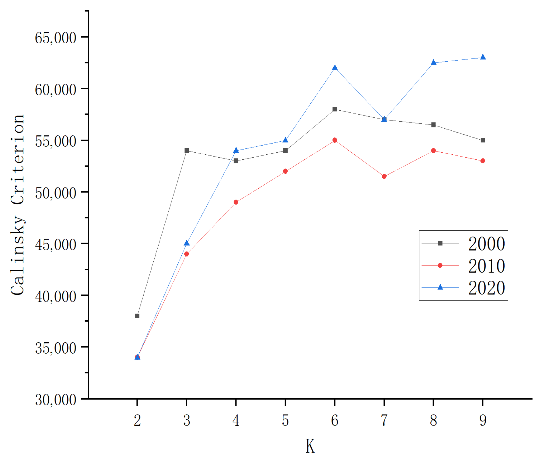
Based on the evaluation of candidate clusters ranging from K = 2 to 10, Figure 3 identifies K = 6 as the optimal partition for this study. The observed peak in the CH criterion at this point serves as statistical validation for the results, confirming that a six-bundle classification maximizes inter-group distinction and intra-group consistency, thus ensuring an objective categorization. The resulting ESBs were visualized using ArcGIS Pro 3.0.0 to analyze their spatiotemporal dynamics and structural characteristics. This systematic identification of ESBs in the Taihu Basin provides an empirical foundation for refined ecological management and scientific planning of functional zones.

2.3.5. Driving Force Analysis

GeoDetector offers a robust technical framework for evaluating how environmental determinants influence spatial distribution configurations, allowing for the quantitative assessment of explanatory power regarding specific phenomena [64]. In this study, five ESs are dependent variables, whereas associated natural and anthropogenic elements serve as independent variables. Following rigorous collinearity screening and data reliability verification, the GeoDetector model was implemented using R software (Version 4.3.3, R Core Team, Vienna, Austria) to elucidate the underlying driving mechanisms shaping ESs. The chosen natural parameters encompass temperature (TEP), soil type (ST), soil depth (SD), PM_2.5 (PM), precipitation (PRE), the soil carbon content (SOC), the soil silt content (SSL), the soil coarse content (SCR), NDVI, DEM, slope aspect (ASP), and LULC. The selected social factors are population density (POP), and the landscape composition factors are the proportions of cultivated land (CLP), forestland (FLP), and built-up land (BLP).

3. Results

3.1. Temporal and Spatial Patterns of Ecosystem Services

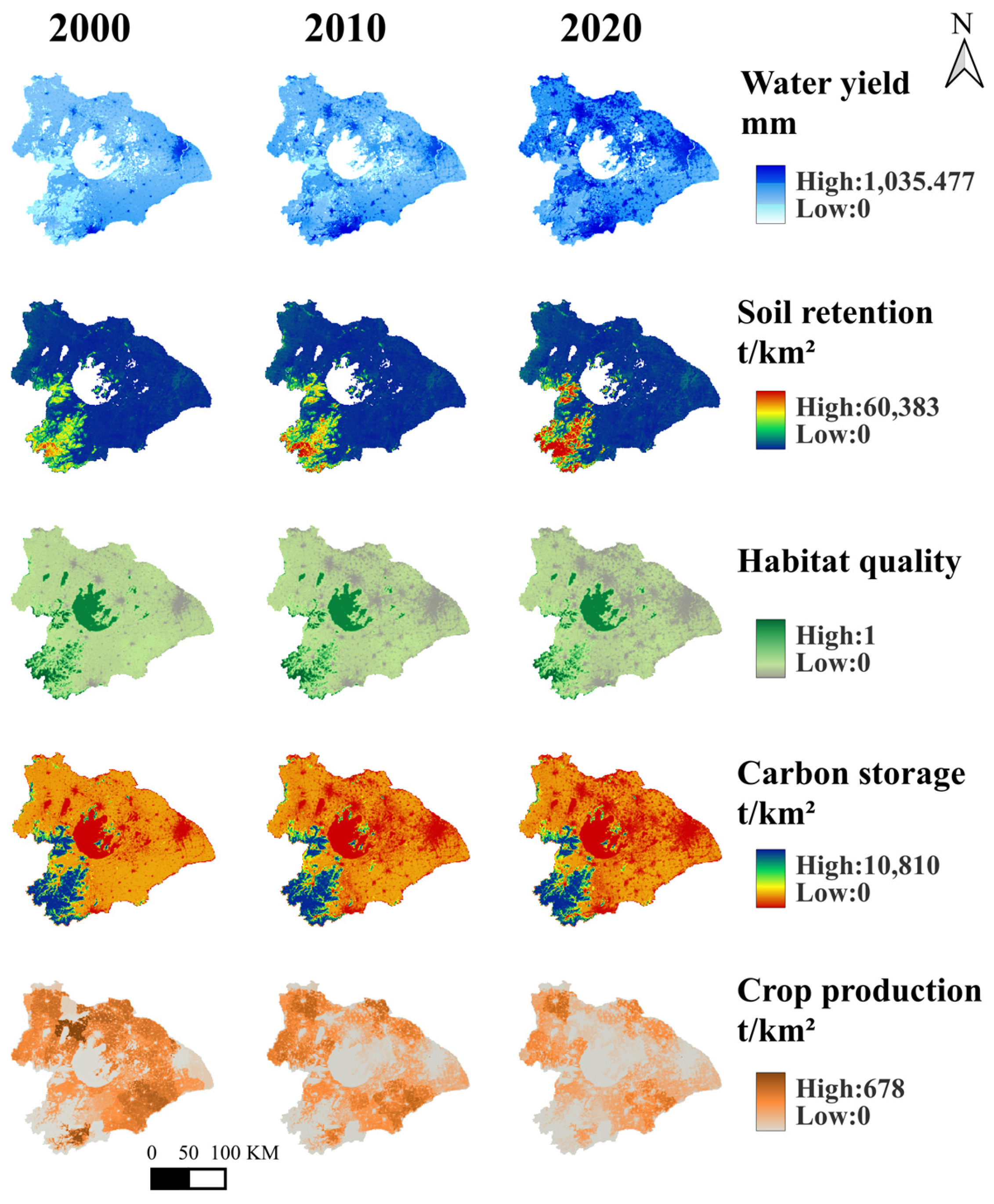
To quantitatively assess five ESs at diverse spatial scales within the Taihu Basin from 2000 to 2020, we utilized the InVEST model combined with the food production model (Figure 4). Significant spatiotemporal heterogeneity was observed among the different ESs.

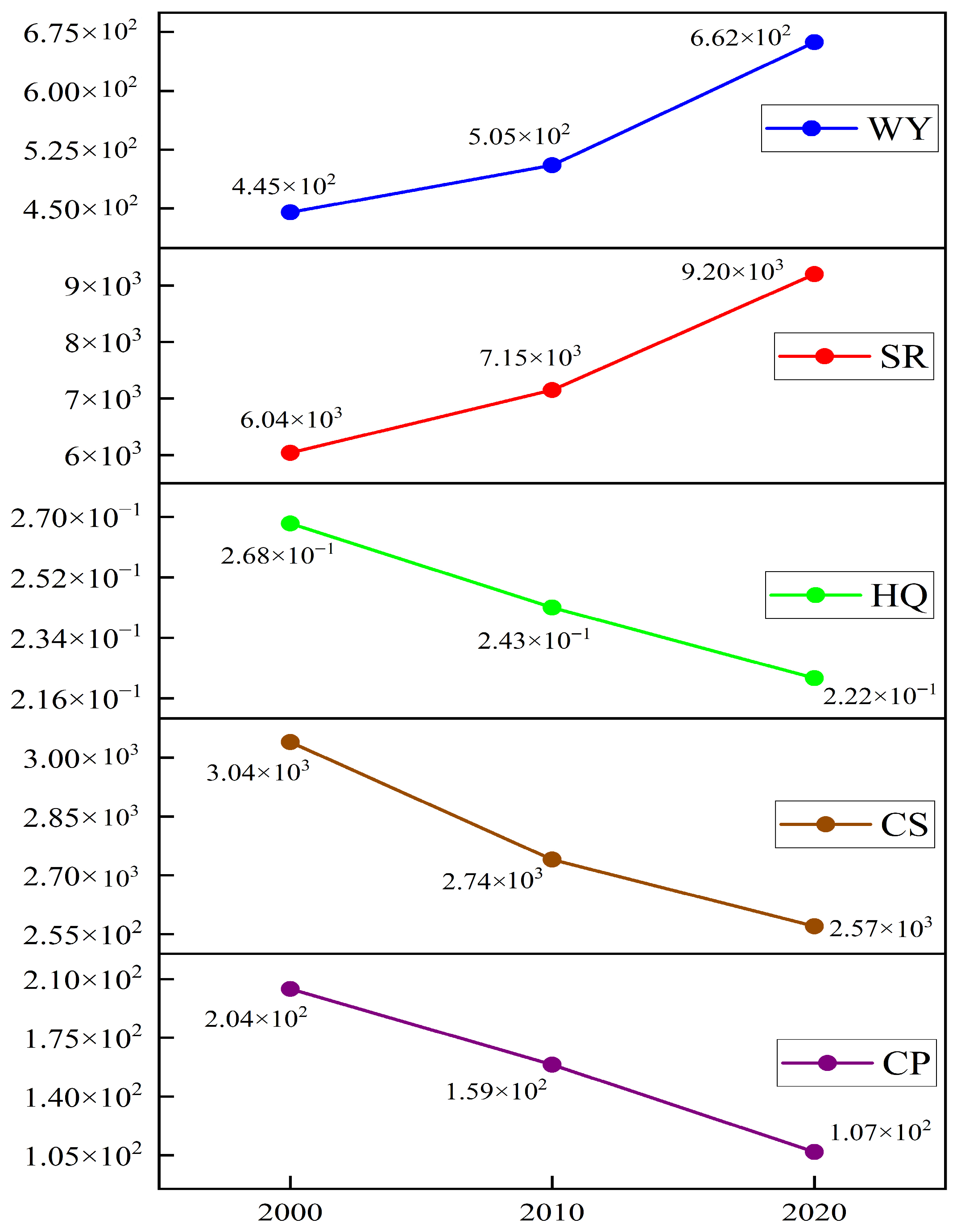
Between 2000 and 2020, the WY and SR significantly increased, increasing by 48.97% and 51.89%, respectively. In contrast, the HQ, CS, and CP all decreased, with growth rates of −17.2%, −15.5%, and −47.6%, respectively (Figure 5). Spatially, high WY values were concentrated within urbanized regions such as Shanghai, Suzhou, Wuxi, and Hangzhou, and expanded annually as impervious surfaces replace natural vegetation. Conversely, the southwestern mountainous regions, characterized by extensive forest coverage, served as high-value areas for SR, HQ, and CS. High CP areas peaked in Changzhou between 2000 and 2010 before they shifted to Zhenjiang, which remained a stable center for agricultural production through 2020 (Figure 4).

3.2. Analysis of Ecosystem Service Hotspots

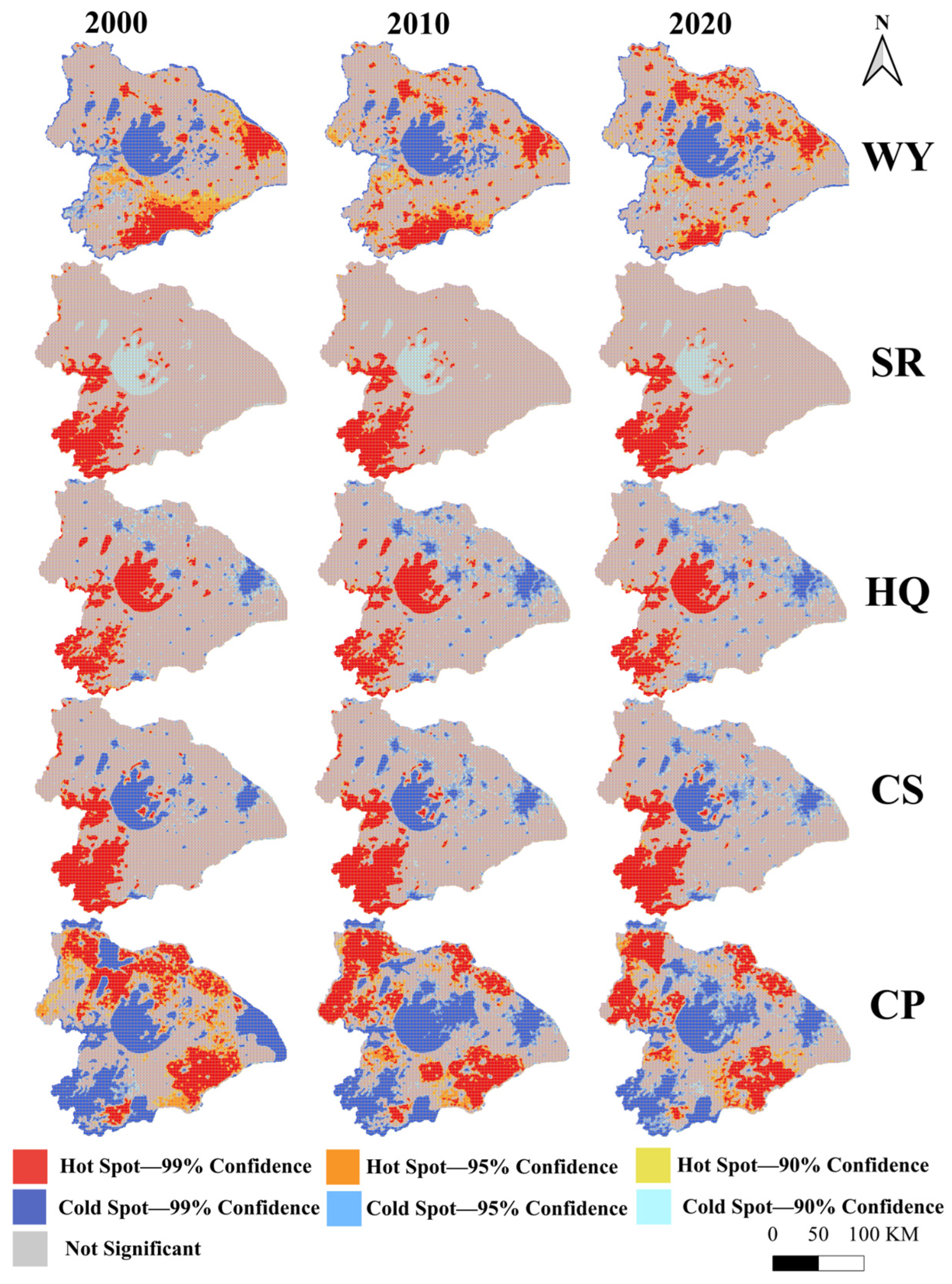
Hotspot analysis via the Getis—Ord Gi* method and Global Moran’s I indicates that the spatial clustering of ESs has intensified over time. Specifically, the Moran’s I for the SR remained high and increased slightly, while the WY, HQ, and CS steadily increased. Most prominently, the index for CP climbed from 0.612 to 0.761, indicating a height increase in spatial aggregation (

Table 3. Outcomes of the global Moran’s I analysis for the Taihu River Basin for 2000 to 2020.

Year	WY	SR	HQ	CS	CP
2000	0.697	0.923	0.784	0.706	0.612
2010	0.678	0.928	0.791	0.722	0.827
2020	0.776	0.931	0.794	0.726	0.761

).

WY hotspots were primarily located in major urban centers such as Shanghai and Hangzhou, with their areal proportion decreasing from 11.9% to 11.83% during the study period. SR and HQ hotspots were largely confined to the southwestern forest patches and the Taihu Lake region; specifically, the area proportion of SR hotspots decreased from 12% to 11.7%, while HQ hotspots declined from 14.3% to 13.4% as urban areas expanded. Similarly, CS hotspots were concentrated in the southwestern forested areas, with their area proportion decreasing from 14.1% to 13.2% while maintaining a stable Moran’s I of approximately 0.71. CP hotspots were mainly distributed in Zhenjiang, Changzhou, and Jiaxing, with their area proportion decreasing from 18.9% to 18.1% (Figure 6).

3.3. Ecosystem Service Tradeoff and Synergy Analysis

3.3.1. Overall Trade-Offs and Synergies Among ESs

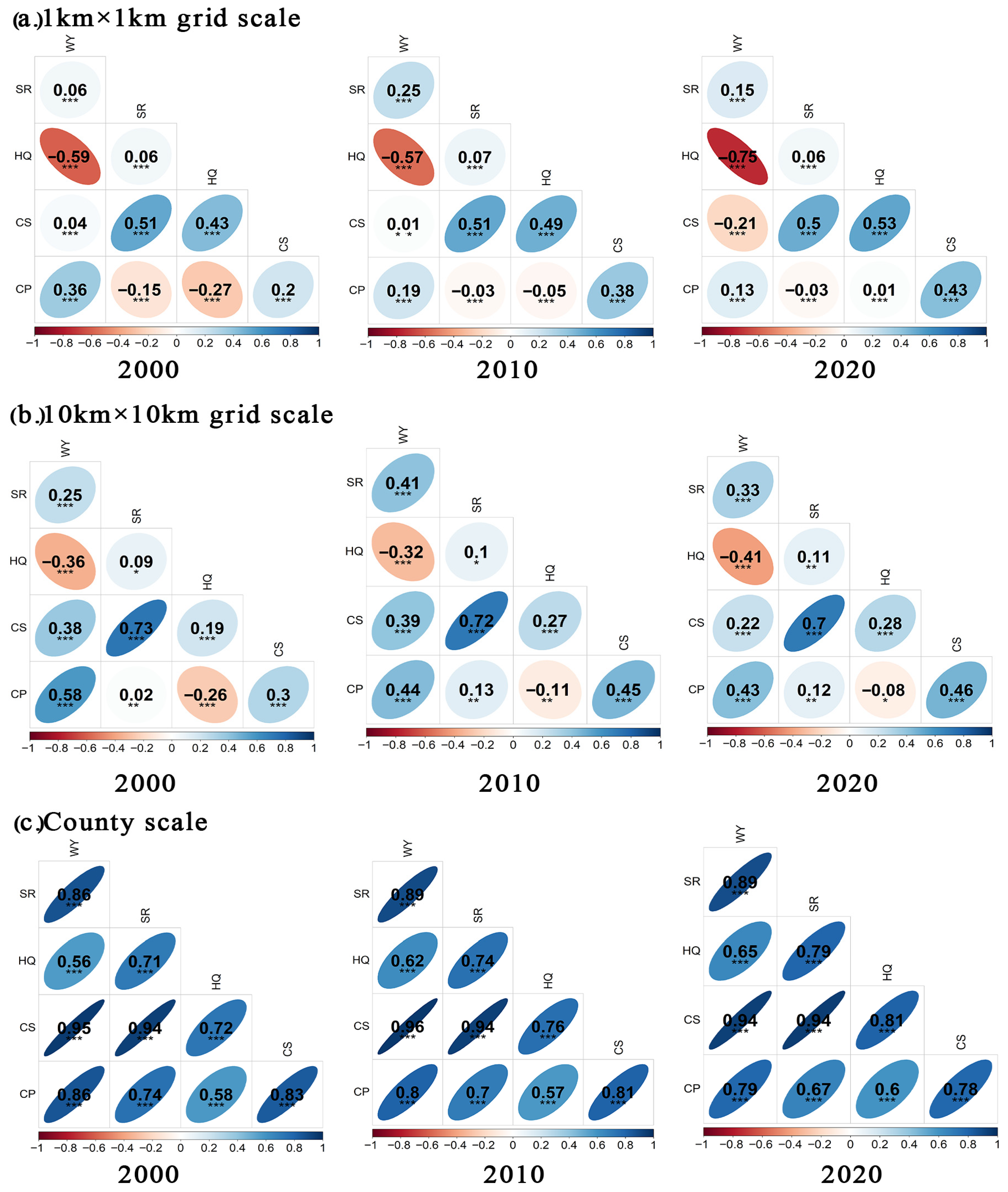
Figure 7 illustrates that as the spatial scale increased, the interactions among ESs transitioned from a trade-off pattern toward synergistic tendencies. Specifically, at the grid scale, the WY and HQ demonstrated a persistent and intense trade-off relationship, which reached its zenith in 2020; As the scale increased, this trade-off gradually diminished. Moreover, the synergy between the SR and CS remained stable and strong, whereas the synergy between the CS and CP increased annually. Additionally, as the grid scale increased, the synergies among SR–CS, CS–CP, WY–SR, WY–CS, and WY–CP continued to increase.

Notably, the synergy between CS and HQ decreases with increasing scale at the grid level, but significant synergy was observed at the county level. At the county level, all ES were strongly positively correlated, with WY–SR, WY–CS, and SR–CS exhibiting particularly strong synergistic relationships. This suggests that at larger scales, land use, climate conditions, and ecological management measures tend to align, enhancing the synergy among ESs, whereas at local scales, resource competition and functional trade-offs are more pronounced.

3.3.2. Spatial Characteristics of the Trade-Offs and Synergies Among ESs

Figure 8 highlights substantial spatial heterogeneity regarding the trade-offs and synergistic interactions among the various ESs at the three spatial scales, revealing five different spatial distribution patterns.

To be specific, WY&SR and HQ&CS demonstrated robust synergistic associations over the vast majority of the area. Regions defined by high synergy between WY and SR were concentrated primarily within the southern sector of the Taihu Basin, notably Hangzhou and Jiaxing, alongside the eastern domain represented by Shanghai, and the western region encompassing Huzhou, Changzhou, and Wuxi. These regions are characterized primarily by developed land and farmland. Additionally, HQ&CS displayed strong synergistic relationships at both the 1 km× 1 km grid scale and the county scale, particularly for developed land, for which the synergistic relationship was notably strong. However, at the 10 km × 10 km grid scale, the synergistic intensity decreased, and the number of unrelated areas increased.

The spatial distributions of the trade-offs and synergies between WY&HQ and SR&HQ were similar. At the 1 km× 1 km grid scale, most areas exhibited weak trade-offs, with strong trade-offs and strong synergies scattered throughout the study region. At the 10 km× 10 km grid scale, the number of unrelated areas significantly increased, and these areas were characterized primarily by weak and moderate trade-offs, with synergistic areas present in a scattered distribution. In most regions, at the county level, the distribution was characterized predominantly by weak trade-offs.

The trade-offs and synergistic relationships between WY&CS and SR&CS also displayed similarities. At the 1 km× 1 km grid scale, most areas exhibited weak trade-offs, with synergistic relations occurring mainly in the western and eastern parts of the Taihu Basin. Strong trade-off areas were scattered throughout the basin, and at the 10 km× 10 km grid scale, strong trade-off and synergy areas disappeared. At the county scale, most regions exhibited weak trade-offs. Notably, the trade-off relationships in the southwestern part of Hangzhou at the county scale were strong for the SR&CS. This phenomenon may be attributed to significant fluctuations in vegetation changes in Lin’an district, Hangzhou, between 2000 and 2020 [65]. Studies have shown that after vegetation restoration measures are implemented, the SR may recover relatively quickly, whereas the response of the CS tends to be delayed response because of the time lag in vegetation accumulation [66], resulting in a trade-off between the two services.

The spatial patterns of the trade-offs and synergies between WY&CP and SR&CP were also quite similar. At all three scales, the synergistic areas were located primarily in the central (including Suzhou and Huzhou), eastern (including Shanghai’s Pudong New Area), and northwestern (including Changzhou and Wuxi) parts of the Taihu Lake Basin.

As the scale increased, the synergistic areas became more concentrated, whereas the trade-off areas remained dispersed. At the county scale, the overall trade-off and synergy effects decreased, and strong trade-off and synergy relationships ceased to exist.

Similarly, the overall spatial configurations for the trade-offs and synergies between CS&CP resembled those of HQ&CP. At the 1 km× 1 km grid scale, the southwest exhibited a potent trade-off, yet this dynamic evolved into a synergistic bond as the scale expanded. Both the 1 km× 1 km grid and county scales displayed distinct synergistic ties in the north, whereas this synergy faded at the 10 km grid scale.

3.4. Identification and Analysis of Ecosystem Service Bundles

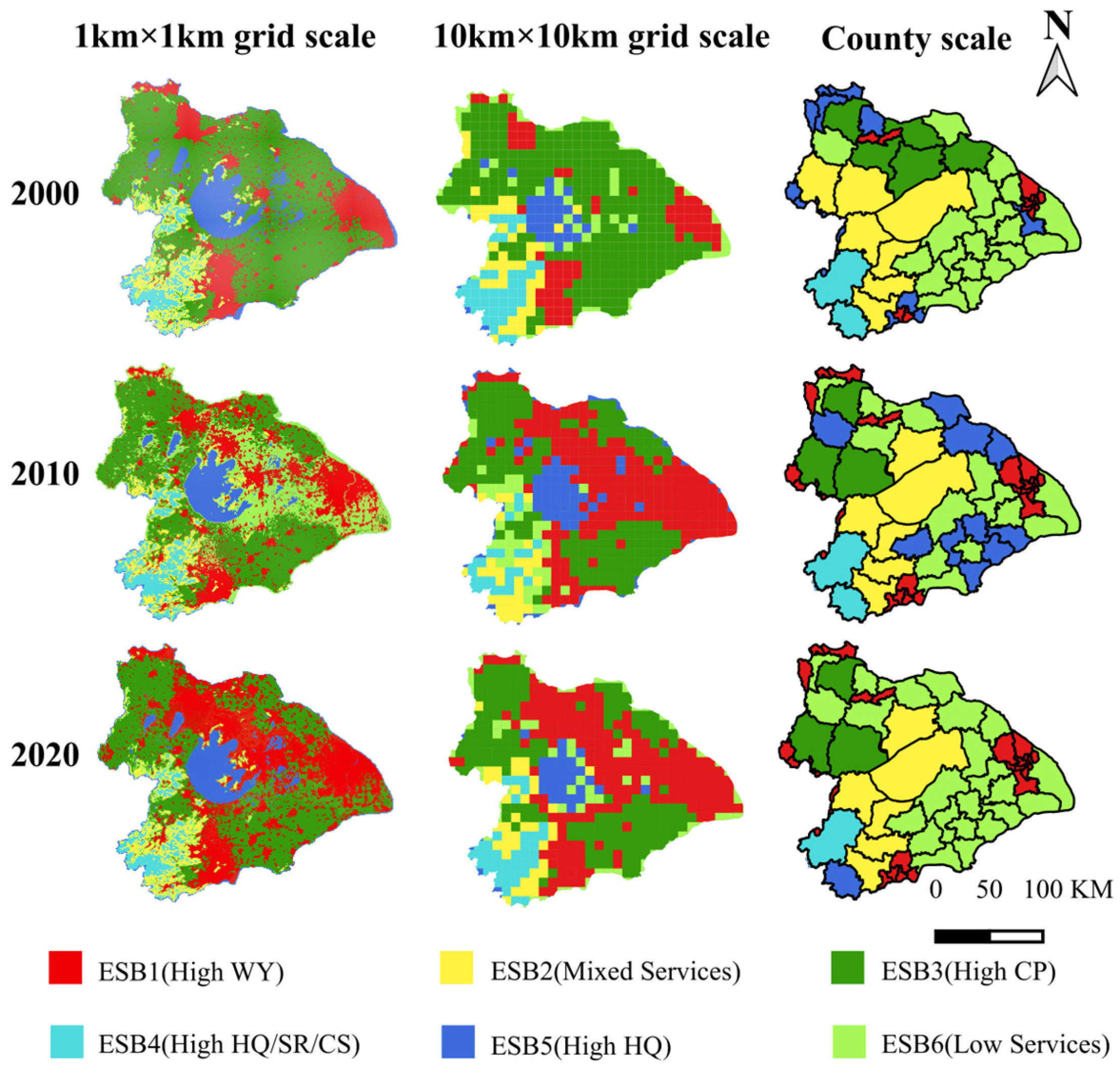
According to the k-means clustering results under the CH criterion, the Taihu Basin was divided into six types of ESBs, and their spatial distribution clearly showed scale heterogeneity (Figure 9). We found that the structural stability of ESBs depends largely on the homogeneity of the landscape. ESBs located in uniform areas, such as continuous forests or urban centers, maintained a stable structure because their dominant ESs persist regardless of the observation scale. Conversely, ESBs situated in complex transition zones were highly unstable. In these interface areas where human activity and nature mix, changing the scale alters the proportion of different land uses, causing the bundle structure to shift significantly.

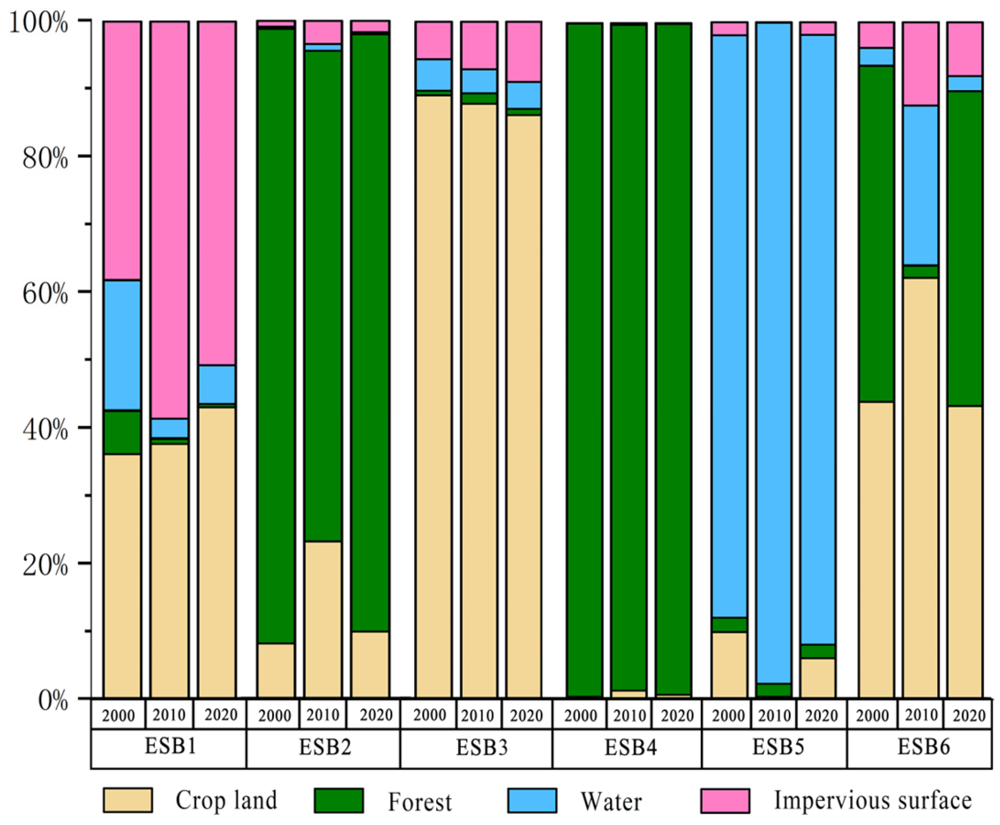
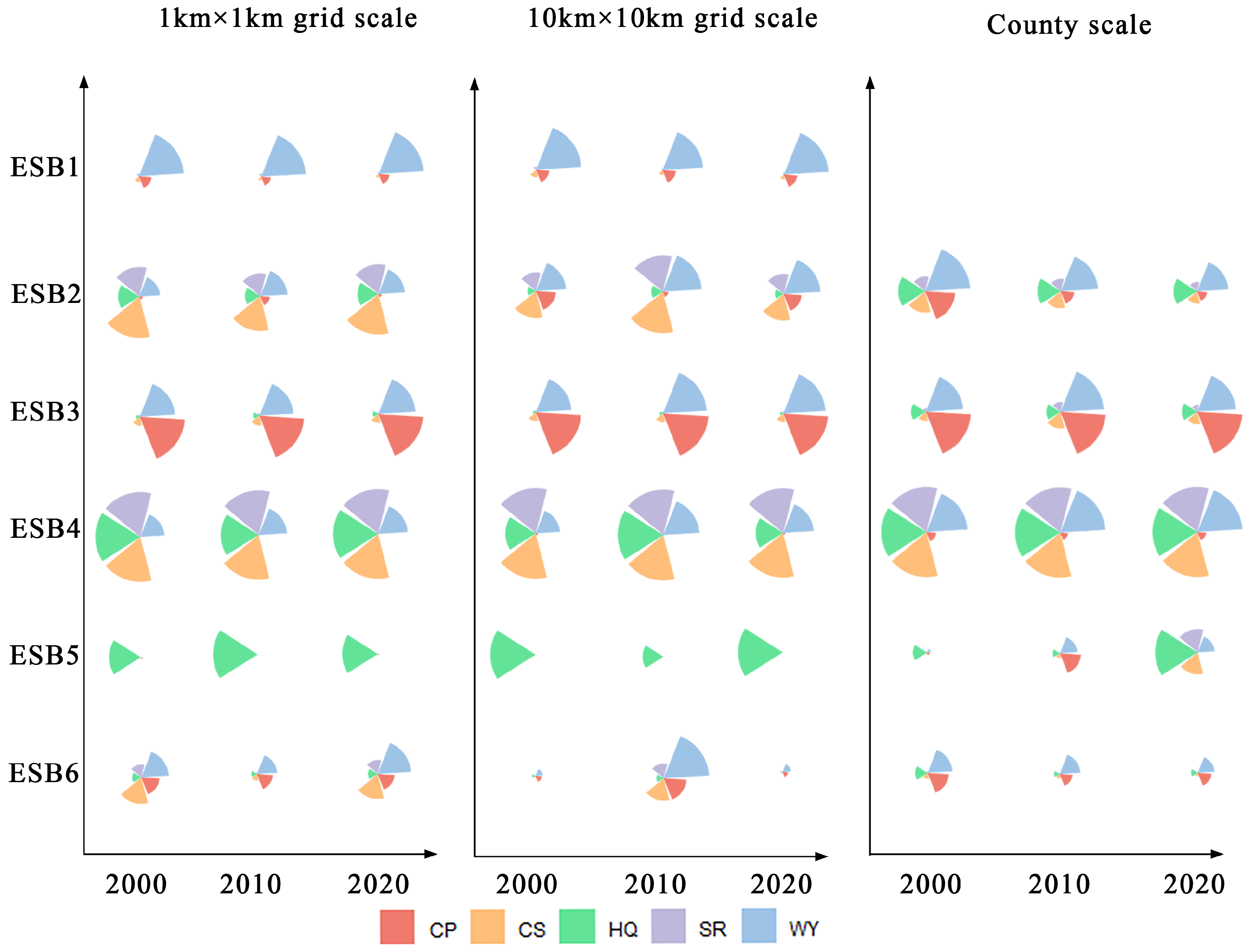
ESB 1, which is driven primarily by the WY, was widely distributed in areas with high levels of urbanization, where the main land use types were impermeable surfaces and farmland (Figure 10). From 2000 to 2020, ESB 1 expanded from an initial point-like distribution to a larger, contiguous area (Figure 9). At the grid scale, the spatial structure of this ESB has remained relatively stable; however, at the county scale, the ES values were generally low (Figure 11).

ESB 2 was primarily found in the forestland fringe areas of the southwestern part of the Taihu Lake Basin, where the main land use types were forestland and cropland (Figure 10). At the 1 km× 1 km grid scale, the primary services were SR, CS, HQ, and WY, with their service structures remaining stable over time. At the 10 km× 10 km grid scale, the HQ value has decreased, whereas the CP services increased. At the county scale, all five services were present, with WY remaining relatively stable and SR and CS showing downward trends (Figure 11).

ESB 3 was dominated by CP and WY, and this bundle is distributed mainly in the middle, eastern and northern regions of the Taihu Lake Basin, where the main land use type was cropland (Figure 10). At multiple spatiotemporal scales, the structure of ESB 3 was relatively stable, and the ecosystem services were highly consistent.

ESB 4 had high levels of ESs other than CP (Figure 11), and this bundle was primarily distributed in the mountainous and hilly areas of the southwestern Taihu Basin (Figure 9). The predominant land use type was forestland (Figure 10). At all the scales, this ESB demonstrated high synergy among HQ, SR, CS, and WY, indicating excellent comprehensive ecosystem regulation capabilities.

ESB 5 was influenced primarily by HQ, with land use consisting mainly of water bodies (Figure 10). At the grid scale, this ESB was stable, provided HQ services, and was concentrated in lake and marsh areas. However, at the county scale, HQ has rapidly declined since 2000 and almost disappeared by 2010 (Figure 11). By 2020, it had recovered, with its distribution center shifting from lake areas to the southwestern forest region of the watershed (Figure 9).

ESB 6 had the weakest overall ecosystem service supply capabilities across all the scales and displayed significant spatial heterogeneity. At the 1 km scale, it was associated with natural tourist attractions in the southwest, while at the 10 km scale, it encompassed low-service areas near eastern built-up regions (Figure 9). At the county scale, the WY and CP values in this bundle decreased annually. The persistent weakness of service functions in these areas, particularly regarding soil erosion, highlights a potential risk of regime shifts and necessitates urgent ecological restoration interventions.

3.5. Analysis of the Driving Forces of Ecosystem Services

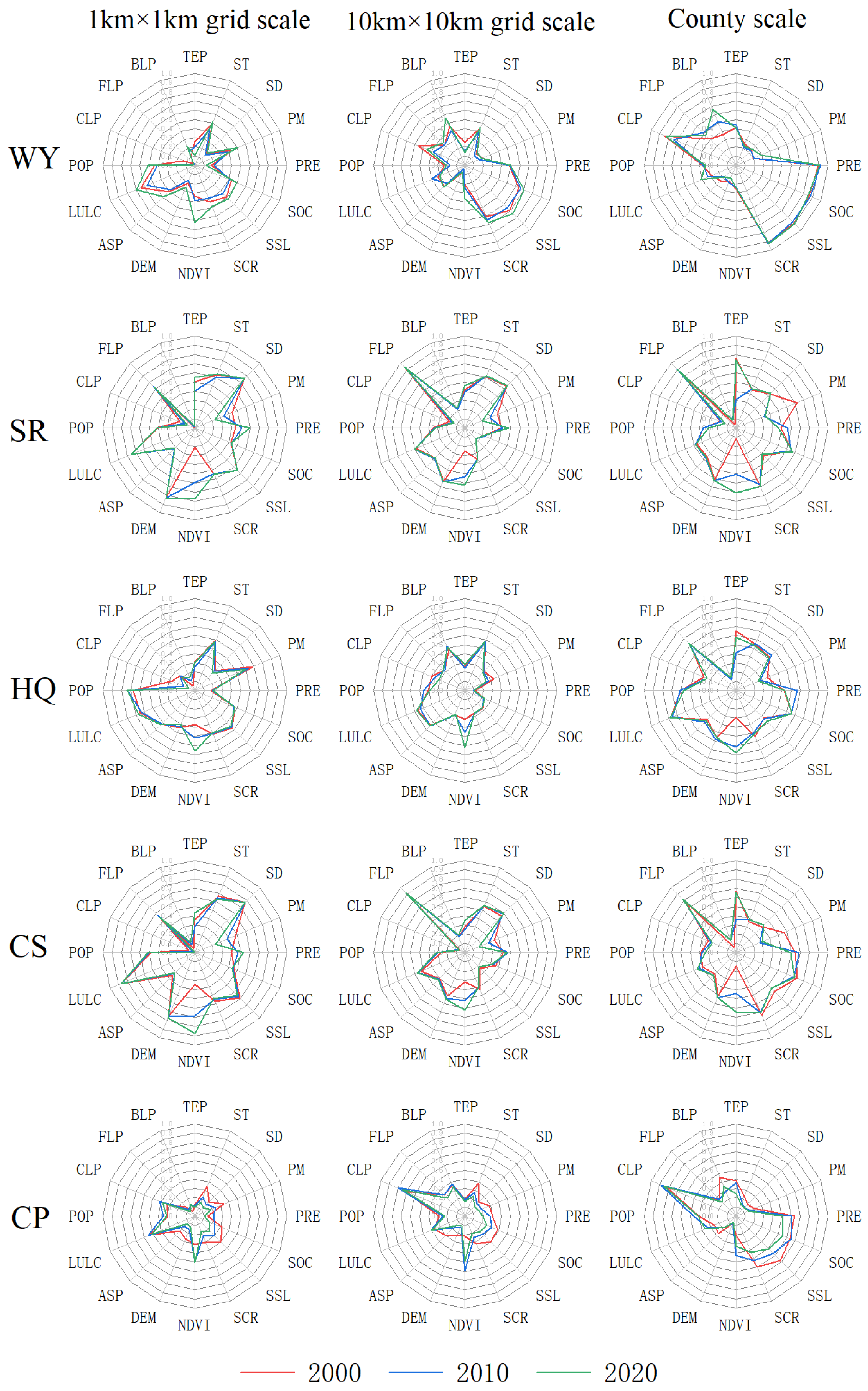
In this study, GeoDetector was applied to examine the drivers of ecosystem services across multiple spatial scales in the Taihu Lake Basin from 2000 to 2020, revealing clear differences in how individual factors influenced Ess (Figure 12). At the grid scale, ESs were primarily regulated by site specific conditions, particularly LULC and topography. As the scale increases, the aggregation process reduced local variability, allowing wider regional influences such as precipitation and landscape composition to emerge as the main controls at the county level.

The GeoDetector results further showed that the strength of different drivers varied with spatial scale. At the 1 km × 1 km grid scale, LULC exerted the greatest control on WY, with a mean q statistic of 0.63 across the study years. At the 10 km × 10 km grid scale, the role of the CLP became more evident, with an average q value of 0.46. At the county scale, PRE and CLP jointly governed the spatial differentiation of water yield, with q values of 0.91 and 0.80, respectively. For SR and CS, FLP consistently represented the dominant factor at all examined scales, with q statistics of 0.63 at 1 km, 0.94 at 10 km, and 0.88 at the county scale. In comparison, slope degree, NDVI, and elevation strongly affected SR and CS at the 1 km × 1 km scale, yet their impacts weakened progressively as the analysis scale increased.

The HQ was primarily controlled by the SD, LULC, and POP, with mean q values of 0.655, 0.575, and 0.567 across the different spatial levels. Regarding the CP, explanatory variables showed limited influence at the 1 km scale where q values remained below 0.3, but the CLP gradually became the key determinant as the scale expanded, with average q values rising to 0.74 at 10 km× 10 km and 0.85 at the county level. In addition, NDVI retained a certain explanatory role for CP at the 10 km× 10 km scale, whereas at the county scale natural factors including PRE, SOC and SSL exerted notable effects. Taken together, variables describing landscape composition exhibited their strongest explanatory capacity at the county scale.

4. Discussion

4.1. Spatiotemporal Evolution of ESs

The Taihu Lake Basin underwent significant ecological changes with divergent trends among services. The most significant upward trend was observed in the WY, which increased by 48.97% over the 20-year study period. From the perspective of urban hydrology [67], this substantial increase is primarily a consequence of land use intensification, where natural vegetation and permeable soils were replaced by impervious surfaces in urban centers such as Shanghai, Suzhou, and Wuxi. This replacement interrupts the natural infiltration—evapotranspiration cycle, shifting the ecosystem into a new state where surface runoff becomes the dominant water pathway. While this increases the calculated WY, it signifies a loss of the internal regulation capacity of the ecosystem, potentially increasing flood vulnerability [68] and substantial risks to groundwater quality [69]. Conversely, CP experienced the most severe degradation, declining rapidly by 47.6%. This sharp decline reflects a fundamental shift in the basin’s economic structure and a clear resource competition for land, where high-yield staple crops are displaced by urban construction or transitioned into higher-value economic crops [70].

The simultaneous increase in the SR of 51.89% suggests that targeted ecological engineering in the southwestern hills effectively mitigated regional soil erosion. However, these findings contrast with the declines in HQ and CS, which show divergent responses among ecosystem services, as reported in other studies [71]. While the SR can be recovered through physical stabilization, the complex biological interactions required for HQ and CS take significantly longer to mature [72]. These findings emphasize that the ecological security of the basin is increasingly dependent on maintaining the integrity of natural patches in the southwest to buffer the environmental pressures generated by the eastern urban core.

4.2. Multiscale Characteristics of the Spatial Patterns of ESs

Spatial scale plays a decisive role in shaping the interactions between ESs. The results show that the overall relationships among ESs gradually transitioned from trade-offs at the 1 km × 1 km grid scale to synergies at the county scale. At the 1 km× 1 km grid scale, landscapes are typically characterized by single land use categories, which promote direct functional competition and mutual exclusion [57,73], as illustrated by the trade-off relationship between WY and HQ (Figure 7). As the grid scale increases, spatial heterogeneity is progressively moderated through a “peak shaving and valley filling” effect [74]. This form of aggregation diminishes the influence of local extremes while emphasizing broader functional integration, thereby reducing trade-offs and strengthening synergies [29,75,76,77,78].

At the county scale, the widespread emergence of strong synergies among most ESs in the overall analysis indicates that administrative governance contributes to system stability [47,79,80]. Within such management units, diversified land-use arrangements enable different services to occupy separate spatial niches, producing an overall synergistic pattern at broader spatial scales. Nevertheless, when the spatial characteristics were analyzed, the relationships observed at the county scale remained largely comparable to those detected at the grid scale. This consistency is also reflected in the distribution of ecosystem service bundles. For instance, ESB4, characterized by relatively high ESs values, remains concentrated in the southwestern counties and sustains the strong synergies among HQ, SR, and CS observed at the grid scale (Figure 8 and Figure 9). Likewise, the continued dominance of ESB1 and ESB3 in eastern and northern regions preserves the trade-offs associated with intensive urbanization and agricultural activities at the county level. Overall, these results indicate that underlying spatial heterogeneity persists even within larger administrative units.

Furthermore, climate variability remains a significant confounding factor; the strong correlations at large scales may be partially driven by regional precipitation patterns rather than by management alone [81], as evidenced by its high explanatory power for WY at the county scale (Figure 12). Recognizing these scale effects is critical for management ecology, as it highlights the risks of applying broad regional policies to local sites where functional trade-offs remain acute and resource competition is most intense.

4.3. Management Implications Based on ESBs

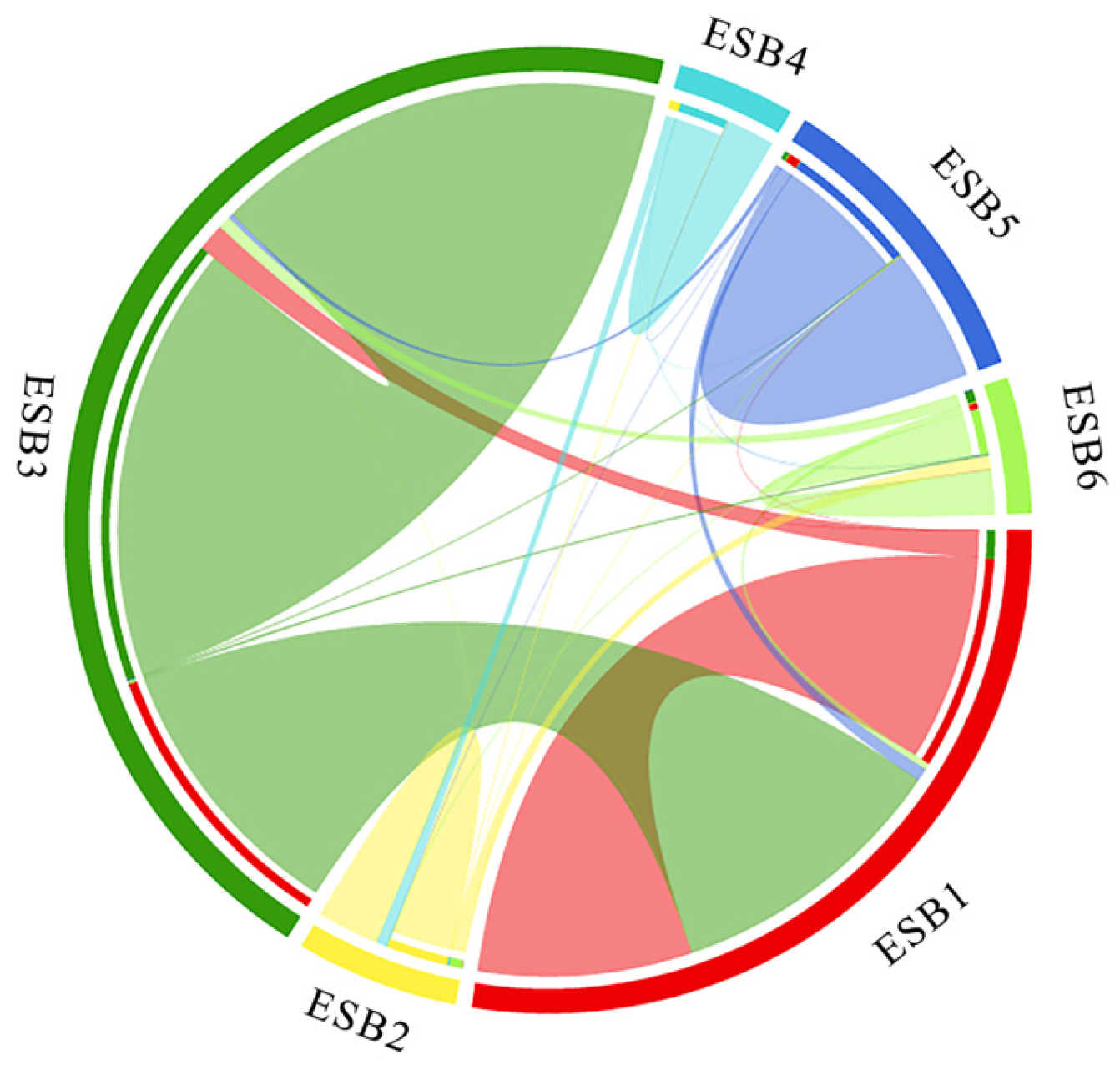
The identification of six distinct ESBs revealed the spatial manifestation of ecological functional groups and provides a scientific basis for refined management in the Taihu Basin. ESB4 exhibited high multifunctional coupling between HQ, SR, and CS. This stability is characteristic of protected forest ecosystems where niche complementarity supports high-level regulating services [16,82]. However, chord diagram analysis (Figure 13) revealed that ESB4 partially transformed into ESB2 at the grid scale between 2000 and 2020. This transition, often found at the forest–farmland interface [83], was likely driven by edge effects and human disturbances, which reduce the structural complexity of forest stands and compromise their regulatory capacity. To mitigate this functional homogenization, management must prioritize maintaining ecosystem connectivity through vegetation restoration between forest patches and performing edge thinning to promote species diversity.

The analysis of ESB1 and ESB5 demonstrates the critical importance of differentiated multiscale management. ESB1, which had the lowest ES values at the county scale, represented areas of severe ecological degradation in the urban cores of Shanghai and Hangzhou [84]. Driven primarily by the WY at the grid scale, ESB1 was heavily influenced by soil factors and LULC. Small-scale ecological restoration, such as the establishment of green corridors with local species, can act as a technical substitute to rehabilitate these degraded urban ecosystems [85]. Conversely, ESB5 was dominated by HQ and was spatially associated with lakes. It was driven by the ST, NDVI, and POP. The transition from ESB4 to ESB5 observed in county located in the southwestern part of the basin at the county scale highlights a decline in ecosystem service intensity [86], indicating emerging risks of forest soil erosion and weakened water regulation.

Furthermore, ESB6 had the weakest overall ES supply. The decline in its service value at the county scale signifies a potential risk of regime shifts [87], where prolonged degradation leads to a permanent loss of ecosystem functions. In the agricultural zones of ESB3, the trade-off between CP and WY was driven by resource competition for water and space during rapid urbanization. To support both yields and hydrologic stability, management must move beyond simple land protection and focus on improving soil health, particularly soil organic carbon and silt content, to increase the soil water storage capacity [88]. By integrating ecological theory with multiscale driver data, regional planning can better balance the basin’s role as an economic powerhouse with the imperative of maintaining resilient ecosystem functions.

4.4. Limitations and Prospects

This study examined the spatial patterns, interactions, and driving mechanisms of ecosystem services at multiple scales in the Taihu Basin, providing insights for regional ecological management. Nevertheless, several limitations remain. First, this study concentrated on five representative ESs due to limitations in data availability, while several other important functions, including water purification, climate regulation, and cultural services were not incorporated. Such omissions may constrain a more comprehensive interpretation of ecosystem functioning, and subsequent research should include a wider spectrum of services to better identify potential trade-offs and synergistic relationships. Furthermore, although the spatial scales adopted in this work were selected with reference to established studies, their suitability may differ in regions characterized by distinct ecological settings.

Moreover, the InVEST framework operates on simplified ecological assumptions and depends on deterministic parameter inputs as described in Appendix A. As a result, intrinsic variability in parameter settings may propagate unevenly across spatial levels and may interact with scale-related aggregation processes, thereby affecting the observed strength of trade-offs and synergies. Future investigations should therefore incorporate higher resolution datasets together with process-oriented modelling approaches to enhance the reliability and accuracy of simulations. Finally, this study mainly assessed the effects of individual driving factors, while interactions among multiple factors were not explicitly considered. Further work should apply multifactor and causal inference approaches to better clarify the mechanisms underlying ecosystem service interactions and to support more effective ecological management in the Taihu Basin.

5. Conclusions

This study systematically examined the spatiotemporal evolution of ecosystem services in the Taihu Basin from 2000 to 2020. Unlike previous studies that focused on a single spatial scale, this research analyzes ecosystem service interactions across multiple scales and shows that statistical relationships shift from trade-offs at the local grid scale to more synergistic patterns at the county scale. However, the spatial characteristics of these interactions remain relatively stable, indicating that site-specific trade-offs persist. A key contribution of this study is the identification of scale-dependent mechanisms driving ecosystem services. Local land-use conflicts primarily influence fine-scale trade-offs, whereas landscape composition and climatic factors play an increasingly important role in shaping regional service patterns. The classification of six ecosystem service bundles reveals pronounced spatial heterogeneity within the basin, with forest-dominated southwestern areas characterized by relatively stable regulating services, in contrast to eastern urbanized regions that exhibit lower ecosystem service levels and stronger human disturbance. Based on these findings, this study supports scale-specific and bundle-targeted spatial planning approaches, including strengthened ecological redline protection in biodiversity hotspots and the enhancement of green infrastructure in urban areas, providing practical guidance for balancing urban development and ecological security in the Taihu Basin.

References

1. Costanza, R. Valuing Natural Capital and Ecosystem Services toward the Goals of Efficiency, Fairness, and Sustainability. Ecosyst. Serv. 2020, 43, 101096. [Google Scholar] [CrossRef]
2. Costanza, R.; d’Arge, R.; de Groot, R.; Farber, S.; Grasso, M.; Hannon, B.; Limburg, K. The Value of the World’s Ecosystem Services and Natural Capital. Ecol. Econ. 1998, 25, 3–15. [Google Scholar] [CrossRef]
3. Kadawatha, A.D.; Mecaskey, J.M.; Swab, R.M.; Burns, J.H. Edge Feathering Across Forest-Meadow Ecotones Increases Light Heterogeneity and Understory Plant Diversity. Forests 2025, 16, 441. [Google Scholar] [CrossRef]
4. Costanza, R.; de Groot, R.; Braat, L.; Kubiszewski, I.; Fioramonti, L.; Sutton, P.; Farber, S.; Grasso, M. Twenty Years of Ecosystem Services: How Far Have We Come and How Far Do We Still Need to Go? Ecosyst. Serv. 2017, 28, 1–16. [Google Scholar] [CrossRef]
5. Beddoe, R.; Costanza, R.; Farley, J.; Garza, E.; Kent, J.; Kubiszewski, I.; Martinez, L.; McCowen, T.; Murphy, K.; Myers, N.; et al. Overcoming Systemic Roadblocks to Sustainability: The Evolutionary Redesign of Worldviews, Institutions, and Technologies. Proc. Natl. Acad. Sci. USA 2009, 106, 2483–2489. [Google Scholar] [CrossRef]
6. Benaissa, F.; Bendahmane, I.; Bourfis, N.; Aoulaiche, O.; Alkama, R. Bioindication of Urban Air Polycyclic Aromatic Hydrocarbons Using Petunia Hybrida. Civ. Eng. J. 2019, 5, 1305–1313. [Google Scholar] [CrossRef]
7. Romero, H.; Ihl, M.; Rivera, A.; Zalazar, P.; Azocar, P. Rapid Urban Growth, Land-Use Changes and Air Pollution in Santiago, Chile. Atmos. Environ. 1999, 33, 4039–4047. [Google Scholar] [CrossRef]
8. Sattler, C.; Matzdorf, B. PES in a Nutshell: From Definitions and Origins to PES in Practice—Approaches, Design Process and Innovative Aspects. Ecosyst. Serv. 2013, 6, 2–11. [Google Scholar] [CrossRef]
9. Liu, H.; Hu, Y.; Li, F.; Yuan, L. Associations of Multiple Ecosystem Services and Disservices of Urban Park Ecological Infrastructure and the Linkages with Socioeconomic Factors. J. Clean. Prod. 2018, 174, 868–879. [Google Scholar] [CrossRef]
10. Bennett, E.M.; Peterson, G.D.; Gordon, L.J. Understanding Relationships among Multiple Ecosystem Services. Ecol. Lett. 2009, 12, 1394–1404. [Google Scholar] [CrossRef]
11. Mach, M.E.; Martone, R.G.; Chan, K.M.A. Human Impacts and Ecosystem Services: Insufficient Research for Trade-off Evaluation. Ecosyst. Serv. 2015, 16, 112–120. [Google Scholar] [CrossRef]
12. Su, B.; Liu, M. Coupling Management Ecosystem Service Supply-Supply Trade-Offs and Supply–Demand Trade-Offs: Framework and Practice. Ecol. Indic. 2024, 166, 112258. [Google Scholar] [CrossRef]
13. Cord, A.F.; Bartkowski, B.; Beckmann, M.; Dittrich, A. Towards Systematic Analyses of Ecosystem Service Trade-Offs and Synergies: Main Concepts, Methods and the Road Ahead. Ecosyst. Serv. 2017, 28, 264–272. [Google Scholar] [CrossRef]
14. Pelosi, C.; Goulard, M.; Balent, G. The Spatial Scale Mismatch between Ecological Processes and Agricultural Management: Do Difficulties Come from Underlying Theoretical Frameworks? Agric. Ecosyst. Environ. 2010, 139, 455–462. [Google Scholar] [CrossRef]
15. Mouchet, M.A.; Lamarque, P.; Martín-López, B.; Crouzat, E.; Gos, P.; Byczek, C.; Lavorel, S. An Interdisciplinary Methodological Guide for Quantifying Associations between Ecosystem Services. Glob. Environ. Change 2014, 28, 298–308. [Google Scholar] [CrossRef]
16. Raudsepp-Hearne, C.; Peterson, G.D.; Bennett, E.M. Ecosystem Service Bundles for Analyzing Tradeoffs in Diverse Landscapes. Proc. Natl. Acad. Sci. USA 2010, 107, 5242–5247. [Google Scholar] [CrossRef]
17. Renard, D.; Rhemtulla, J.M.; Bennett, E.M. Historical Dynamics in Ecosystem Service Bundles. Proc. Natl. Acad. Sci. USA 2015, 112, 13411–13416. [Google Scholar] [CrossRef]
18. Qi, N.; Sun, W.; Kan, H.; Liu, L.; Zou, J.; Pang, Z.; Zhang, G. Evaluation on Water-Related Ecosystem Services of Minyun Reservoir During 2008–2019. Bull. Soil Water Conserv. 2021, 41, 276–283+291. [Google Scholar]
19. Wu, C.; Ma, G.; Yang, W.; Zhou, Y.; Peng, F.; Wang, J.; Yu, F. Assessment of Ecosystem Service Value and Its Differences in the Yellow River Basin and Yangtze River Basin. Sustainability 2021, 13, 3822. [Google Scholar] [CrossRef]
20. Shah, S.M.; Liu, G.; Yang, Q.; Wang, X.; Casazza, M.; Agostinho, F.; Lombardi, G.V.; Giannetti, B.F. Emergy-Based Valuation of Agriculture Ecosystem Services and Dis-Services. J. Clean. Prod. 2019, 239, 118019. [Google Scholar] [CrossRef]
21. Francesconi, W.; Srinivasan, R.; Pérez-Miñana, E.; Willcock, S.P.; Quintero, M. Using the Soil and Water Assessment Tool (SWAT) to Model Ecosystem Services: A Systematic Review. J. Hydrol. 2016, 535, 625–636. [Google Scholar] [CrossRef]
22. Gao, J.; Li, F.; Gao, H.; Zhou, C.; Zhang, X. The Impact of Land-Use Change on Water-Related Ecosystem Services: A Study of the Guishui River Basin, Beijing, China. J. Clean. Prod. 2017, 163, S148–S155. [Google Scholar] [CrossRef]
23. Martínez-López, J.; Bagstad, K.J.; Balbi, S.; Magrach, A.; Voigt, B.; Athanasiadis, I.; Pascual, M.; Willcock, S.; Villa, F. Towards Globally Customizable Ecosystem Service Models. Sci. Total Environ. 2019, 650, 2325–2336. [Google Scholar] [CrossRef]
24. Yin, L.; Zheng, W.; Shi, H.; Ding, D. Ecosystem Services Assessment and Sensitivity Analysis Based on ANN Model and Spatial Data: A Case Study in Miaodao Archipelago. Ecol. Indic. 2022, 135, 108511. [Google Scholar] [CrossRef]
25. Lin, S.; Wu, R.; Yang, F.; Wang, J.; Wu, W. Spatial Trade-Offs and Synergies among Ecosystem Services within a Global Biodiversity Hotspot. Ecol. Indic. 2018, 84, 371–381. [Google Scholar] [CrossRef]
26. Wang, Z. Satellite-Observed Effects from Ozone Pollution and Climate Change on Growing-Season Vegetation Activity over China during 1982–2020. Atmosphere 2021, 12, 1390. [Google Scholar]
27. Feng, Q.; Zhao, W.; Hu, X.; Liu, Y.; Daryanto, S.; Cherubini, F. Trading-off Ecosystem Services for Better Ecological Restoration: A Case Study in the Loess Plateau of China. J. Clean. Prod. 2020, 257, 120469. [Google Scholar] [CrossRef]
28. Feng, Z.; Jin, X.; Chen, T.; Wu, J. Understanding Trade-Offs and Synergies of Ecosystem Services to Support the Decision-Making in the Beijing–Tianjin–Hebei Region. Land Use Policy 2021, 106, 105446. [Google Scholar]
29. Zeng, S.; Jiang, C.; Bai, Y.; Wang, H.; Liu, E.; Guo, L.; Chen, S.; Zhang, J. Understanding Scale Effects and Differentiation Mechanisms of Ecosystem Services Tradeoffs and Synergies Relationship: A Case Study of the Lishui River Basin, China. Ecol. Indic. 2024, 167, 112648. [Google Scholar] [CrossRef]
30. Liao, J.; Yu, C.; Feng, Z.; Zhao, H.; Wu, K.; Ma, X. Spatial Differentiation Characteristics and Driving Factors of Agricultural Eco-Efficiency in Chinese Provinces from the Perspective of Ecosystem Services. J. Clean. Prod. 2021, 288, 125466. [Google Scholar] [CrossRef]
31. Vallet, A.; Locatelli, B.; Levrel, H.; Wunder, S.; Seppelt, R.; Scholes, R.J.; Oszwald, J. Relationships Between Ecosystem Services: Comparing Methods for Assessing Tradeoffs and Synergies. Ecol. Econ. 2018, 150, 96–106. [Google Scholar] [CrossRef]
32. Xia, H.; Yuan, S.; Prishchepov, A.V. Spatial-Temporal Heterogeneity of Ecosystem Service Interactions and Their Social-Ecological Drivers: Implications for Spatial Planning and Management. Resour. Conserv. Recycl. 2023, 189, 106767. [Google Scholar] [CrossRef]
33. Grafius, D.R.; Corstanje, R.; Harris, J.A. Linking Ecosystem Services, Urban Form and Green Space Configuration Using Multivariate Landscape Metric Analysis. Landsc. Ecol. 2018, 33, 557–573. [Google Scholar] [CrossRef] [PubMed]
34. Kettani, O.; Ramdani, F.; Tadili, B. AK-Means: An Automatic Clustering Algorithm Based on K-Means. J. Adv. Comput. Sci. Technol. 2015, 4, 231–236. [Google Scholar] [CrossRef]
35. Wang, Z.; Gao, Y.; Zhang, X.; Li, L.; Li, F. Integrating Historical Patterns and Future Trends for Ecological Management Zone Identification and Validation: A Case Study in Beijing, China. Sci. Total Environ. 2024, 927, 172249. [Google Scholar] [CrossRef]
36. Warchalska-Troll, A.; Warchalski, T. The Selection of Areas for Case Study Research in Socio-Economic Geography with the Application of k-Means Clustering. Wiad. Stat. Pol. Stat. 2022, 67, 1–20. [Google Scholar] [CrossRef]
37. Xu, X.; Yu, J.; Wang, F. Analysis of Ecosystem Service Drivers Based on Interpretive Machine Learning: A Case Study of Zhejiang Province, China. Environ. Sci. Pollut. Res. 2022, 29, 64060–64076. [Google Scholar] [CrossRef]
38. Geng, W.; Li, Y.; Zhang, P.; Yang, D.; Jing, W.; Rong, T. Analyzing Spatio-Temporal Changes and Trade-Offs/Synergies among Ecosystem Services in the Yellow River Basin, China. Ecol. Indic. 2022, 138, 108825. [Google Scholar] [CrossRef]
39. Huang, Y.; Wu, J. Spatial and Temporal Driving Mechanisms of Ecosystem Service Trade-off/Synergy in National Key Urban Agglomerations: A Case Study of the Yangtze River Delta Urban Agglomeration in China. Ecol. Indic. 2023, 154, 110800. [Google Scholar] [CrossRef]
40. Rimal, B.; Sharma, R.; Kunwar, R.; Keshtkar, H.; Stork, N.E.; Rijal, S.; Rahman, S.A.; Baral, H. Effects of Land Use and Land Cover Change on Ecosystem Services in the Koshi River Basin, Eastern Nepal. Ecosyst. Serv. 2019, 38, 100963. [Google Scholar] [CrossRef]
41. Long, H.; Liu, Y.; Hou, X.; Li, T.; Li, Y. Effects of Land Use Transitions Due to Rapid Urbanization on Ecosystem Services: Implications for Urban Planning in the New Developing Area of China. Habitat Int. 2014, 44, 536–544. [Google Scholar] [CrossRef]
42. Luo, Y.; Yang, D.; O’Connor, P.; Wu, T.; Ma, W.; Xu, L.; Guo, R.; Lin, J. Dynamic Characteristics and Synergistic Effects of Ecosystem Services under Climate Change Scenarios on the Qinghai–Tibet Plateau. Sci. Rep. 2022, 12, 2540. [Google Scholar] [CrossRef] [PubMed]
43. Shen, J.; Zhao, M.; Tan, Z.; Zhu, L.; Guo, Y.; Li, Y.; Wu, C. Ecosystem Service Trade-Offs and Synergies Relationships and Their Driving Factor Analysis Based on the Bayesian Belief Network: A Case Study of the Yellow River Basin. Ecol. Indic. 2024, 163, 112070. [Google Scholar] [CrossRef]
44. Li, R.; Zheng, H.; O’Connor, P.; Xu, H.; Li, Y.; Lu, F.; Robinson, B.E.; Ouyang, Z.; Hai, Y.; Daily, G.C. Time and Space Catch up with Restoration Programs That Ignore Ecosystem Service Trade-Offs. Sci. Adv. 2021, 7, eabf8650. [Google Scholar] [CrossRef]
45. Hou, X.; Yang, H.; Cao, J. The Spatial and Temporal Characteristics of Ecosystem Service Trade-Offs and Synergistic Relationships in a Mountainous Region of Northern China. ISPRS Int. J. GEO-Inf. 2024, 13, 458. [Google Scholar] [CrossRef]
46. Chen, Y.; Liu, W.; Zhao, F.; Zhao, Q.; Xu, Z.; Asiedu Kumi, M. Multi-Scale Analysis of Ecosystem Service Trade-Offs/Synergies in the Yangtze River Delta. Land 2024, 13, 1462. [Google Scholar] [CrossRef]
47. Zhou, J.; Yang, J.; Tang, Z.; Xue, L.; Zhang, W.; Zhang, J. Driving Mechanisms of Ecosystem Services and Their Trade-Offs and Synergies in the Transition Zone between the Qinghai-Tibet Plateau and the Loess Plateau. Ecol. Indic. 2025, 171, 113148. [Google Scholar] [CrossRef]
48. Pu, J.; Shen, A.; Liu, C.; Wen, B. Impacts of Ecological Land Fragmentation on Habitat Quality in the Taihu Lake Basin in Jiangsu Province, China. Ecol. Indic. 2024, 158, 111611. [Google Scholar] [CrossRef]
49. Du, J.; Gong, Y.; Xi, X.; Liu, C.; Qian, C.; Ye, B. The Study on the Spatiotemporal Changes in Tradeoffs and Synergies of Ecosystem Services and Response to Land Use/Land Cover Changes in the Region around Taihu Lake. Heliyon 2024, 10, e33375. [Google Scholar] [CrossRef]
50. Bai, Y.; Chen, Y.; Alatalo, J.M.; Yang, Z.; Jiang, B. Scale Effects on the Relationships between Land Characteristics and Ecosystem Services- a Case Study in Taihu Lake Basin, China. Sci. Total Environ. 2020, 716, 137083. [Google Scholar] [CrossRef]
51. Taihu Basin Authority of MWR. Water Resources Bulletin of Taihu Basin in 2020. Available online: https://www.tba.gov.cn/slbthlyglj/upload/1cd25cf6-fcc6-4ec8-873b-b041dacfd0c7.pdf (accessed on 7 April 2025).
52. Zhou, Y.; Li, H.; Wu, W.; Zhang, L.; Zhu, H.; Naren, T. Mapping Taihu Basin Research: A Bibliometric Analysis. Environ. Rev. 2021, 29, 391–400. [Google Scholar] [CrossRef]
53. Yan, F.; Shangguan, W.; Zhang, J.; Hu, B. Depth-to-Bedrock Map of China at a Spatial Resolution of 100 Meters. Sci. Data 2020, 7, 2. [Google Scholar] [CrossRef] [PubMed]
54. Growing-Season NDVI over China During 1982–2020. Available online: https://www.scidb.cn/en/detail?dataSetId=905485350665715712&version=V1 (accessed on 7 February 2026).
55. Yang, J.; Huang, X. The 30 m Annual Land Cover Datasets and Its Dynamics in China from 1985 to 2022. Natl. Cryosphere Desert Data Cent. 2023. [Google Scholar] [CrossRef]
56. Polasky, S.; Nelson, E.; Pennington, D.; Johnson, K.A. The impact of land-use change on ecosystem services, biodiversity and returns to landowners: A case study in the state of Minnesota. Environ. Resour. Econ. 2011, 48, 219–242. [Google Scholar] [CrossRef]
57. Shen, J.; Li, S.; Liu, L.; Liang, Z.; Wang, Y.; Wang, H.; Wu, S. Uncovering the relationships between ecosystem services and social-ecological drivers at different spatial scales in the Beijing-Tianjin-Hebei region. J. Clean. Prod. 2021, 290, 125193. [Google Scholar] [CrossRef]
58. Getis, A.; Ord, J.K. The Analysis of Spatial Association by Use of Distance Statistics. Geogr. Anal. 1992, 24, 189–206. [Google Scholar] [CrossRef]
59. An, Z.; Sun, C.; Hao, S. Spatial heterogeneity and driving forces of ecosystem services: An individual-pair-bundle perspective. J. Geogr. Sci. 2025, 35, 2039–2068. [Google Scholar] [CrossRef]
60. Li, H.; Calder, C.A.; Cressie, N. Beyond Moran’s I: Testing for spatial dependence based on the spatial autoregressive model. Geogr. Anal. 2007, 39, 357–375. [Google Scholar] [CrossRef]
61. Li, S.; Zhang, C.; Liu, J.; Zhu, W.; Ma, C.; Wang, J. The tradeoffs and synergies of ecosystem services: Research progress, development trend, and themes of geography. Geogr. Res. 2013, 32, 1379–1390. [Google Scholar]
62. Queiroz, C.; Meacham, M.; Richter, K.; Norström, A.V.; Andersson, E.; Norberg, J.; Peterson, G. Mapping Bundles of Ecosystem Services Reveals Distinct Types of Multifunctionality within a Swedish Landscape. AMBIO 2015, 44, 89–101. [Google Scholar] [CrossRef]
63. Caliński, T.; Harabasz, J. A dendrite method for cluster analysis. Commun. Stat.-Theory Methods 1974, 3, 1–27. [Google Scholar] [CrossRef]
64. Zeng, W.; Wan, X.; Lei, M.; Gu, G.; Chen, T. Influencing Factors and Prediction of Arsenic Concentration in Pteris Vittata: A Combination of Geodetector and Empirical Models. Environ. Pollut. 2022, 292, 118240. [Google Scholar] [CrossRef] [PubMed]
65. Hangzhou Municipal People’s Government. Natural Disturbance-Based Forest Management. Available online: https://www.hangzhou.gov.cn/art/2024/9/13/art_812262_59102513.html (accessed on 14 December 2024).
66. Su, H.; Du, M.; Liu, Q.; Kang, X.; Zhao, L.; Zheng, W.; Liao, Z. Assessment of Regional Ecosystem Service Bundles Coupling Climate and Land Use Changes. Ecol. Indic. 2024, 169, 112844. [Google Scholar] [CrossRef]
67. Oswald, C.J.; Kelleher, C.; Ledford, S.H.; Hopkins, K.G.; Sytsma, A.; Tetzlaff, D.; Toran, L.; Voter, C. Integrating urban water fluxes and moving beyond impervious surface cover: A review. J. Hydrol. 2023, 618, 129188. [Google Scholar] [CrossRef]
68. Zhang, Q.; Li, C.; Wen, D.; Kang, J.; Chen, T.; Zhang, B.; Hu, Y.; Yin, J. Global South shows higher urban flood exposures than the Global North under current and future scenarios. Commun. Earth Environ. 2025, 6, 594. [Google Scholar] [CrossRef]
69. Motlagh, A. Urban Stormwater and Groundwater Quality: Pathways, Risks, and Green Infrastructure Solutions. Environments 2025, 12, 446. [Google Scholar] [CrossRef]
70. Cao, X.; Han, J.; Li, X. Analysis of the impact of land use change on grain production in Jiangsu Province. China Land 2023, 13, 20. [Google Scholar] [CrossRef]
71. Zhao, L.; Xin, W.; Mao, X.; Shao, D.; Chen, Q.; Zhu, Y.; Han, F. Trade-off relationships of ecosystem services for soil retention carbon sinks in the Loess Plateau of China. Land Use Policy 2025, 158, 107751. [Google Scholar] [CrossRef]
72. Feng, X.; Fu, B.; Lu, N.; Zeng, Y.; Wu, B. How ecological restoration alters ecosystem services: An analysis of carbon sequestration in China’s Loess Plateau. Sci. Rep. 2013, 3, 2846. [Google Scholar] [CrossRef]
73. Yang, Y.; Zheng, H.; Kong, L.; Huang, B.; Xu, W.; Ouyang, Z. Mapping ecosystem services bundles to detect high-and low-value ecosystem services areas for land use management. J. Clean. Prod. 2019, 225, 11–17. [Google Scholar] [CrossRef]
74. Hou, Y.; Lü, Y.; Chen, W.; Fu, B. Temporal variation and spatial scale dependency of ecosystem service interactions: A case study on the central Loess Plateau of China. Landsc. Ecol. 2017, 32, 1201–1217. [Google Scholar] [CrossRef]
75. Chang, B.; Chen, B.; Chen, W.; Xu, S.; He, X.; Yao, J.; Huang, Y. Analysis of trade-off and synergy of ecosystem services and driving forces in urban agglomerations in Northern China. Ecol. Indic. 2024, 165, 112210. [Google Scholar] [CrossRef]
76. Chen, J.; He, S.; Xue, J.; Zhang, H.; Li, Z.; Wang, L.; Li, K. Exploring ecosystem service trade-offs and their response to landscape configuration at multi-scales: A case study of Hubei Province. Acta Ecol. Sin. 2023, 43, 4835–4846. [Google Scholar] [CrossRef]
77. Pei, Y.j.; Luo, M.y.; Zhao, Y.h.; Han, L.; Yang, S.y.; Zhang, L. Trade-offs and synergies among ecosystem services at multiple scales: A case study of Yan’an City. Chin. J. Ecol. 2022, 41, 1351–1360. [Google Scholar]
78. Xu, S.; Liu, Y.; Wang, X.; Zhang, G. Scale effect on spatial patterns of ecosystem services and associations among them in semi-arid area: A case study in Ningxia Hui Autonomous Region, China. Sci. Total Environ. 2017, 598, 297–306. [Google Scholar] [CrossRef]
79. Ostrom, E. A general framework for analyzing sustainability of social-ecological systems. Science 2009, 325, 419–422. [Google Scholar] [CrossRef]
80. Feng, X.; Zhao, L.; Ma, T.; Zhao, Z.; Hu, B. Scale effects on ecosystem service interactions and driving factors in the three river source basin: Insights and management implications. Water 2024, 16, 3425. [Google Scholar] [CrossRef]
81. Wu, S.; Li, R.; Yan, Y.; Du, Z.; Wu, Z.; Ma, K. Scale-dependent drivers of ecosystem service supply-flow-demand couplings in the Shanxi Yellow River Basin, China. iScience 2025, 28, 114002. [Google Scholar] [CrossRef]
82. Hooper, D.U.; Chapin, F.S., III; Ewel, J.J.; Hector, A.; Inchausti, P.; Lavorel, S.; Lawton, J.H.; Lodge, D.M.; Loreau, M.; Naeem, S.; et al. Effects of biodiversity on ecosystem functioning: A consensus of current knowledge. Ecol. Monogr. 2005, 75, 3–35. [Google Scholar] [CrossRef]
83. Haddad, N.M.; Brudvig, L.A.; Clobert, J.; Davies, K.F.; Gonzalez, A.; Holt, R.D.; Lovejoy, T.E.; Sexton, J.O.; Austin, M.P.; Collins, C.D.; et al. Habitat fragmentation and its lasting impact on Earth’s ecosystems. Sci. Adv. 2015, 1, e1500052. [Google Scholar] [CrossRef]
84. Cai, Y.B.; Li, H.M.; Ye, X.Y.; Zhang, H. Analyzing three-decadal patterns of land use/land cover change and regional ecosystem services at the landscape level: Case study of two coastal metropolitan regions, Eastern China. Sustainability 2016, 8, 773. [Google Scholar] [CrossRef]
85. Klaus, V.H.; Kiehl, K. A conceptual framework for urban ecological restoration and rehabilitation. Basic Appl. Ecol. 2021, 52, 82–94. [Google Scholar] [CrossRef]
86. Huang, C.; Cheng, X.; Zhang, Z. Future land use and habitat quality dynamics: Spatio-temporal analysis and simulation in the taihu lake basin. Sustainability 2024, 16, 7793. [Google Scholar] [CrossRef]
87. Crépin, A.S.; Biggs, R.; Polasky, S.; Troell, M.; De Zeeuw, A. Regime shifts and management. Ecol. Econ. 2012, 84, 15–22. [Google Scholar] [CrossRef]
88. Rawls, W.; Pachepsky, Y.A.; Ritchie, J.; Sobecki, T.; Bloodworth, H. Effect of soil organic carbon on soil water retention. Geoderma 2003, 116, 61–76. [Google Scholar] [CrossRef]
89. Yang, D.; Liu, W.; Tang, L.; Chen, L.; Li, X.; Xu, X. Estimation of Water Provision Service for Monsoon Catchments of South China: Applicability of the InVEST Model. Landsc. Urban Plan. 2019, 182, 133–143. [Google Scholar] [CrossRef]
90. Campolongo, F.; Cariboni, J.; Saltelli, A. An Effective Screening Design for Sensitivity Analysis of Large Models. Environ. Model. Softw. 2007, 22, 1509–1518. [Google Scholar] [CrossRef]
91. Zhu, C.; Zhang, X.; Zhou, M.; He, S.; Gan, M.; Yang, L.; Wang, K. Impacts of Urbanization and Landscape Pattern on Habitat Quality Using OLS and GWR Models in Hangzhou, China. Ecol. Indic. 2020, 117, 106654. [Google Scholar] [CrossRef]
92. Ding, T. Assessment of Coordinative Relationship between Comprehensive Ecosystem Service and Urbanization: A Case Study of Yangtze River Delta Urban Agglomerations, China. Ecol. Indic. 2021, 133, 108454. [Google Scholar] [CrossRef]
93. Zhang, X.; Wang, J.; Yue, C.; Ma, S.; Wang, L.-J. Exploring the Spatiotemporal Changes in Carbon Storage under Different Development Scenarios in Jiangsu Province, China. PeerJ 2022, 10, e13411. [Google Scholar] [CrossRef]
94. Chang, X.; Xing, Y.; Wang, J.; Yang, H.; Gong, W. Effects of Land Use and Cover Change (LUCC) on Terrestrial Carbon Stocks in China between 2000 and 2018. Resour. Conserv. Recycl. 2022, 182, 106333. [Google Scholar] [CrossRef]
95. Yang, J.; Huang, X. The 30m Annual Land Cover Dataset and Its Dynamics in China from 1990 to 2019. Earth Syst. Sci. Data 2021, 13, 3907–3925. [Google Scholar] [CrossRef]
96. Zhou, H.; Tang, M.; Huang, J.; Zhang, J.; Huang, J.; Zhao, H.; Yu, Y. Instability and Uncertainty of Carbon Storage in Karst Regions under Land Use Change: A Case Study in Guiyang, China. Front. Environ. Sci. 2025, 13, 1551050. [Google Scholar] [CrossRef]
97. Nunez, J.A.; Aguiar, S.; Jobbagy, E.G.; Jimenez, Y.G.; Baldassini, P. Climate Change and Land Cover Effects on Water Yield in a Subtropical Watershed Spanning the Yungas-Chaco Transition of Argentina. J. Environ. Manag. 2024, 358, 120808. [Google Scholar] [CrossRef] [PubMed]
98. Goyal, M.K.; Khan, M. Assessment of Spatially Explicit Annual Water-Balance Model for Sutlej River Basin in Eastern Himalayas and Tungabhadra River Basin in Peninsular India. Hydrol. Res. 2016, 48, 542–558. [Google Scholar] [CrossRef]
99. Abdelwahab, O.M.M.; Ricci, G.F.; Netti, A.M.; Girolamo, A.M.D.; Gentile, F. Modeling the Effect of Nature-Based Solutions in Reducing Soil Erosion with InVEST® SDR: The Carapelle Case Study. Water 2025, 17, 3451. [Google Scholar] [CrossRef]
100. Tamire, C.; Elias, E.; Argaw, M. Spatiotemporal Dynamics of Soil Loss and Sediment Export in Upper Bilate River Catchment (UBRC), Central Rift Valley of Ethiopia. Heliyon 2022, 8, e11220. [Google Scholar] [CrossRef]
101. Vigiak, O.; Borselli, L.; Newham, L.T.H.; McInnes, J.; Roberts, A.M. Comparison of Conceptual Landscape Metrics to Define Hillslope-Scale Sediment Delivery Ratio. Geomorphology 2012, 138, 74–88. [Google Scholar] [CrossRef]
102. Xie, X.; Peng, M.; Zhang, L.; Chen, M.; Li, J.; Tuo, Y. Assessing the Impacts of Climate and Land Use Change on Water Conservation in the Three-River Headstreams Region of China Based on the Integration of the InVEST Model and Machine Learning. Land 2024, 13, 352. [Google Scholar] [CrossRef]
Figure 1. (a) Location, extent, and elevation of the research region (red area: Taihu Lake Basin, China); (b) LULC in 2000; (c) LULC in 2010; (d) LULC in 2020.
Sustainability 18 02930 g001
Figure 2. Research framework.
Sustainability 18 02930 g002
Figure 3. Calinski criterion values under different numbers of clusters.
Sustainability 18 02930 g003
Figure 4. Spatial distribution patterns of five ecosystem services (WY, SR, HQ, CS, and CP) in the Taihu Basin from 2000 to 2020.
Sustainability 18 02930 g004
Figure 5. Divergent temporal trends in ecosystem service provision (2000–2020): WY and SR exhibited growth, whereas HQ, CS, and CP showed declines. (WY: mm, SR/CS/CP: ton/km2, HQ: dimensionless index).
Sustainability 18 02930 g005
Figure 6. Spatiotemporal evolution of Hotspots (High-High clusters, red) and Cold spots (Low-Low clusters, blue) for ecosystem services in the Taihu Basin (2000, 2010, and 2020), based on Getis—Ord Gi* analysis.
Sustainability 18 02930 g006
Figure 7. Spearman correlation matrices showing trade-offs (red circles, negative values) and synergies (blue circles, positive values) among ESs across three spatial scales. The size of the circle and number represent the correlation coefficient (r). (a) 1 km × 1 km grid scale; (b) 10 km × 10 km grid scale; (c) County scale. *, ** and *** indicate significance at the p < 0.05, p < 0.01 and p < 0.001 levels, respectively.
Sustainability 18 02930 g007
Figure 8. Spatial distribution of trade-offs and synergies among ESs in the Taihu Basin (2000–2020) across the 1 km, 10 km, and county scales. Blue indicates synergies, and red indicates trade-offs.
Sustainability 18 02930 g008
Figure 9. Spatiotemporal evolution of ESBs in the Taihu Basin (2000–2020). The maps visualize the spatial configuration of six distinct bundle types derived from K-means clustering analysis, revealing the dynamic shifts in service composition patterns over time.
Sustainability 18 02930 g009
Figure 10. Composition of major Land Use and Land Cover (LULC) types within each ESB at a 1 km× 1 km resolution. The stacked bars illustrate the proportion of different land use categories associated with each bundle type, revealing the distinct spatial correspondence between landscape patterns and service bundles.
Sustainability 18 02930 g010
Figure 11. Compositional profiles of the six ESBs based on min-max normalized means. The rose diagrams display the relative intensity (0–1) of each service, highlighting the distinct functional specialization of each bundle.
Sustainability 18 02930 g011
Figure 12. Quantitative attribution of driving factors for ES using the GeoDetector. The radar charts display the q-statistic values, quantifying the explanatory power of factors at the 1 km × 1 km, 10 km × 10 km, and county scales.
Sustainability 18 02930 g012
Figure 13. Chord Diagram Illustrating ESBs from 2000 to 2020 at the 1 km Scale. The different colors correspond to the distinct Ecosystem Service Bundles (ESB1–ESB6) as labeled on the outer ring, while the colored chords represent the transitions between these bundles.
Sustainability 18 02930 g013