Article

CDT: An Effective Framework for Short-Term Photovoltaic Power Prediction
1
School of Emergency Management Science and Engineering, University of Chinese Academy of Sciences, Beijing 100049, China
2
School of Engineering Science, University of Chinese Academy of Sciences, Beijing 100049, China
*
Author to whom correspondence should be addressed.
Sustainability 2026, 18(6), 2719; https://doi.org/10.3390/su18062719
Submission received: 30 January 2026 / Revised: 28 February 2026 / Accepted: 4 March 2026 / Published: 11 March 2026
(This article belongs to the Special Issue Sustainable Development of Renewable Energy Resources)

Abstract

Increasing the proportion of renewable energy sources, such as photovoltaic power, in the grid can reduce fossil fuel consumption and build a low-carbon power system. However, the inherent instability of the photovoltaic power output makes it difficult to predict, thus increasing the cost of grid operation. Therefore, to improve the accuracy of power prediction and promote the development of the grid, a four-stage short-term photovoltaic power prediction framework, namely, CDT, is proposed, which includes decomposition, classification, reconstruction and forecasting. The initial power data are decomposed using complete ensemble empirical mode decomposition with adaptive noise. Next, an improved data classification and reconstruction method based on dynamic time warping is developed to process the data, which reduces the dimensionality of the data while preserving trend information. Finally, the reconstructed components are predicted using the improved TCN model. The results of the empirical study show that the proposed CDT has higher precision and scalability in processing and predicting the trend of photovoltaic power generation, compared to the other benchmark models.

1. Introduction

Solar energy, as a clean and renewable resource, can address society’s ever-increasing demand for electricity. Over the past three decades, global photovoltaic (PV) technology and industry have advanced rapidly, achieving significant breakthroughs in both theoretical and applied research. PV power generation offers extensive application scenarios, with solar panels capable of flexible deployment and utilization in both urban and rural settings. For example, Xiao et al. proposed utilizing PV systems to power electric buses while selling surplus electricity, which not only effectively reduces carbon emissions but also promotes sustainable operations for urban public transportation [1]. Compared to traditional energy generation methods, PV power generation requires relatively less land area and can be deployed across diverse geographical conditions. This makes it an energy form suitable for various terrains and geographic environments. With continuous technological advancement and maturation, the cost of PV generation has steadily decreased, making it competitive and capable of providing consumers with more economical electricity supply. Furthermore, the fuel costs required for generation are virtually zero, rendering it unaffected by factors like international oil prices and reducing the risk of energy cost volatility.
Against the background of renewable energy gradually becoming a vital component of the global energy structure, PV power forecasting holds significant importance in modern energy management. However, PV systems exhibit characteristics such as intermittency and volatility, with their generation capacity strongly influenced by meteorological conditions like solar irradiance and temperature. Accurate PV power forecasting provides a reliable basis for power system dispatch, thereby enhancing system stability. When PV generation capacity can be predicted in advance, power systems can better allocate generation resources. During periods of high generation, PV energy can be prioritized to ensure supply-demand balance, preventing power shortages or surpluses caused by inadequate planning. By predicting PV panel output, operators can optimize operational strategies, such as adjusting panel operating states and scheduling timely maintenance, to ensure normal operation and enhance generation efficiency. Furthermore, accurate forecasting empowers operators to develop more flexible electricity trading strategies, participate in power markets, and enhance economic benefits.
Artificial intelligence has emerged as a pivotal solution, with recent research constructing energy scheduling systems [2], and deploying data-driven deep learning models for PV forecasting [3]. Traditional and classic neural network models, such as convolutional neural network, Long short-term memory network and Gated Recurrent Unit, have long been applied in this field [4,5,6]. Ouyang et al. conducted feature analysis and parameter optimization for regional PV plant clustering, dissecting the clustering dimensions of PV generation consistency. They established a K-means clustering model for PV plants that integrates spatio-temporal characteristics and inherent plant properties. Subsequently, they constructed LSTM-based prediction models for each cluster to achieve regional PV generation forecasting [7]. Zhang et al. focused on the impact of weather conditions such as sunny and cloudy days on PV generation. They developed a short-term PV forecasting method based on sunny-day decomposition and TCN. This approach identifies the photovoltaic output from the most recent sunny day for the target date and combines it with sunny-day component removal techniques to decompose the photovoltaic power waveform [8]. Aman et al. similarly considered different weather conditions, employing CNN layers to identify weather states such as sunny and cloudy days. Subsequently, they utilized LSTM layers to learn solar power generation patterns influenced by weather variations, thereby enabling power forecasting. This hybrid model comprehensively incorporates multiple meteorological factors to enhance the accuracy of photovoltaic power forecasting [9]. Some researches group and integrate pre-screen scenarios with similar photovoltaic power outputs prior to data forecasting to enhance data relevance. Yang et al. proposes an innovative photovoltaic power forecasting model that mitigates network degradation and enhances the usability of numerical weather prediction. They firstly handled PV output data based on Elkan K-means algorithm and Mahalanobis distance, and then established a bidirectional recurrent residual network to extract the temporal features of photovoltaic output [10]. Sun et al. proposed a weather classification algorithm based on multi-scale fluctuation characteristics to select meteorological data, and extracted the spatio-temporal correlation of different PV sites by multi-channel structured long and short-term neural network modeling method to realize the prediction [11].
However, in PV generation forecasting, traditional deep learning methods typically process these sequences individually, significantly reducing model prediction efficiency. Furthermore, as PV plants expand and forecasting demands increase, this approach may result in slow prediction speeds, making it difficult to meet real-time forecasting requirements. Consequently, some researchers have incorporated the intrinsic geographical correlations among multiple influencing factors, such as irradiance and temperature, within power generation data. By integrating graph neural networks, they have achieved PV forecasting [12]. Zhuang et al. first leveraged the multi-output capability of the Informer model to ensure predictions for long sequence data. Simultaneously, they extracted feature information from nodes via a graph convolutional module, enhancing the reliability of prediction results [13]. Guan et al. [14] integrated meteorological factors with the spatial correlation of PV plants. They employed a graph attention network to capture spatial relationships between different plants while utilizing CNN to extract meteorological feature information. Subsequently, these two types of feature information were fused and input into an improved LSTM model based on Spiking Neural P Systems to extract PV generation temporal features and complete the prediction task.
The above studies predominantly utilize the original sensor data without systematically extracting embedded trends and fluctuation patterns. To investigate the trend of PV output data, a non-stationary time series, some scholars have introduced signal decomposition methods [15,16,17,18]. Liu et al. employed the interquartile range method to detect outliers and utilized multiple techniques to fill missing values in the data. They then constructed an ultra-short-term PV generation prediction model based on wavelet decomposition, a dual-attention mechanism, and BiLSTM. During forecasting, wavelet decomposition effectively handles the volatility and nonlinear characteristics of PV generation data [19]. Wu et al. noted the volatility and forward information leakage issues during sequence stacking. Building upon the use of the Spearman feature selector to screen sequence features, they incorporated a variational modal decomposition layer into the Informer encoder to decompose feature sequences and reduce their volatility. Finally, replacing the self-attention distillation mechanism with an expanded causal convolutional layer, which both extends the receptive field and ensures the causality of time series predictions [20]. Wu et al. first partitioned data into multiple sub-sequences using CEEMDAN. They then quantified the complexity of each sub-sequence by sample entropy, reorganized sub-sequences with similar entropy values to reduce computational load, and finally proposed a hybrid CNN-GRU neural network for prediction [21]. The examples show that the prediction model that combines signal decomposition and deep networks better captures the information of the PV output sequence. Although these strategies have partially worked on the exactness of the prediction, there remains considerable space for additional improvement.
Traditional deep neural networks often suffer from issues such as insufficient feature extraction capabilities, local optima, slow convergence, and poor prediction results. To address these challenges, researchers have begun exploring methods for neural network hyperparameter tuning. In recent years, intelligent optimization algorithms have attracted widespread attention [16,18,22]. Sun et al. modified Archimedean optimization approach to address the challenges associated with calibrating model parameters [11]. Li et al. employed Catch Fish Optimization Algorithm to adjust hyperparameters in CNN-BiLSTM [23]. Souhe et al. integrated machine learning with neural networks, proposing a prediction method combining Support Vector Machines and Gated Recurrent Units. They utilized Ant Colony Optimization to achieve synergistic optimization, enabling the model to attain optimal predictive performance [24].
Despite this prominent progress, current hybrid forecasting frameworks still exhibit several critical gaps. First, while signal decomposition techniques effectively mitigate data volatility, most existing studies blindly feed all decomposed Intrinsic Mode Functions (IMFs) into prediction models without further processing, significantly increasing computational overhead. Second, studies that do attempt to classify IMFs often rely on subjective, arbitrary empirical thresholds, lacking a rigorous, data-driven mathematical standard. Finally, traditional temporal models often treat all time steps equally, lacking the mechanism to focus dynamically on abrupt meteorological changes.
To address these limitations, this paper proposes a data-driven CEEMDAN and DTW-based TCN short-term PV power prediction framework named CDT. The principal contributions are summarized as follows:
(1) An objective, data-driven sequence classification strategy is proposed to bridge the gap between signal decomposition and prediction. Unlike conventional subjective thresholding, we utilize Dynamic Time Warping (DTW) to quantify the similarity between CEEMDAN-decomposed IMFs and solar irradiance. Subsequently, the K-Means clustering algorithm is employed to objectively categorize these sub-sequences into three physically interpretable components, long-term trend, medium-term fluctuation, and short-term volatility. This strategy eliminates human bias, preserves multi-scale temporal features, and significantly reduces computational dimensionality.
(2) By integrating an attention mechanism into the Temporal Convolutional Network, the model dynamically focuses on the most critical meteorological time steps. Furthermore, the Grey Wolf Optimization algorithm is introduced to automate hyperparameter configuration, avoiding sub-optimal empirical settings and achieving a synergistic balance between computational efficiency and sequential modeling depth.
(3) Comprehensive ablation and comparative experiments are conducted. Validated on two real-world datasets spanning diverse weather conditions, the proposed framework demonstrates superior robustness. Experimental results indicate that the framework effectively reduces the Mean Absolute Error (MAE) by 21.4% and improves the R 2 by 1% compared to conventional benchmark models.
Section 2 describes methods used in this paper. Section 3 illustrates the data sources and experiments. Section 4 draws the conclusion.

2. Methodology

2.1. Data Decomposition

Photovoltaic power generation is influenced by multiple factors including solar irradiance, temperature, season, and terrain. These factors are all mixed within the same time-domain curve, exhibiting nonlinear, non-stationary, and abrupt characteristics. Direct application of neural network prediction models struggles to accurately capture these patterns of change. To address this issue, we first decomposes the original data to reduce its complexity and extract key information and features before performing the prediction. Common signal processing methods include empirical modal decomposition (EMD) and VMD. However, each of these methods has its own limitations: EMD is prone to modal aliasing during the decomposition process, resulting in multiple frequency components in the intrinsic mode function (IMF), which reduces the interpretability of the decomposition results. VMD is based on the principle of variational decomposition and achieves signal decomposition through iterative optimization, but its effectiveness is greatly affected by the number of modes and the manual setting of the penalty parameter, which limits its applicability.
Compared with them, complete ensemble empirical mode decomposition with adaptive noise (CEEMDAN) [25] introduces adaptive noise, which eliminates the problem of residual noise while avoiding mode aliasing. CEEMDAN is also able to effectively separate the features of PV data in different time scales, facilitating further analysis and data reconstruction.
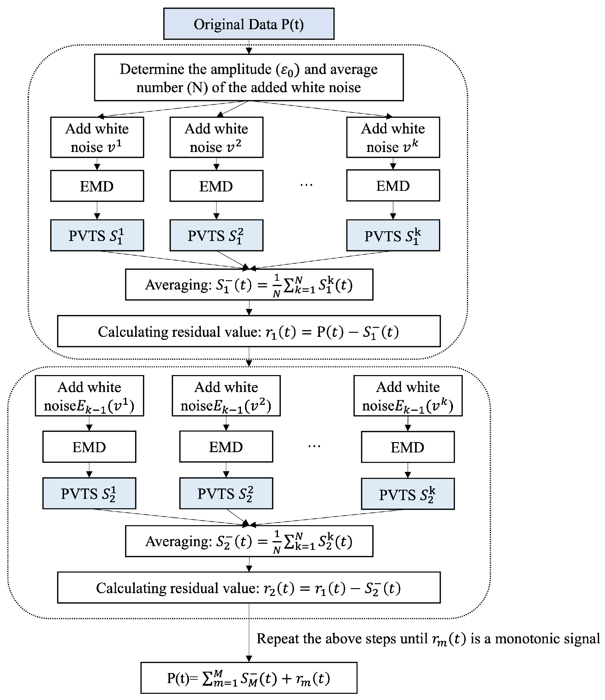
Define P ( t ) = [ p 1 , p 2 , , p n ] as the original PV signal to be decomposed. S i ( · ) is the i-th PV trend subseries (PVTS) obtained by CEEMDAN, and  r k represents the residual component. The workflow of CEEMDAN is presented in Figure 1.
y ( t ) = m = 1 M S m ( t ) + r m ( t )

2.2. Data Classification and Reconstruction

IMFs obtained from CEEMDAN provide detailed characteristics of photovoltaic data across different time scales, revealing fluctuations and trend information. However, CEEMDAN typically decomposes the original signal into over ten IMFs, necessitating their classification and reconstruction of temporal characteristics to provide foundational support for forecasting and scheduling optimization.
We propose a classification-reconstruction stage based on the association between individual PVTS and solar irradiance sequences. Although the Pearson correlation coefficient is conventionally employed to quantify linear interdependencies, its validity relies on strict temporal alignment and linear assumptions. Practical scenarios often exhibit nonlinear relationships or temporal misalignment between specific PVTSs and solar irradiance variations—conditions inadequately addressed by Pearson metrics. In contrast, dynamic time warping (DTW) [26] mitigates these limitations through dynamic temporal realignment. By strategically stretching or compressing subsequences via dynamic programming, DTW optimizes localized sequence matching, thereby generating robust similarity measures. The minimum DTW distance corresponds to maximal similarity in fluctuation patterns, offering enhanced correlation assessment capabilities. Let the solar irradiance sequence be S I = [ s i 1 , s i 2 , , s i n ] . Construct an n × n matrix D, where D ( i , j ) denotes the Euclidean distance between S i and s i j .
D ( i , j ) = S i s i j
Then construct a cumulative distance matrix C, where each element C ( i , j ) denotes the total distance of the shortest path from the starting point (1,1) to (i,j).
C 1 ( i , j ) = D ( i , j ) + m i n C 1 ( i 1 , j ) , C 1 ( i , j 1 ) , C 1 ( i 1 , j 1 ) s . t . C 1 ( 1 , 1 ) = D 1 ( 1 , 1 ) C 1 ( i , 0 ) = C 1 ( 0 , j ) =
After calculating the DTW distance between each IMF and the solar irradiance sequence, the K-Means clustering algorithm is employed to objectively categorize these IMFs into three distinct groups ( k = 3 ) based on their distance magnitudes, thereby avoiding any subjective threshold selection. The first group exhibits smaller DTW distances, reflecting the long-term trend between PV power and solar irradiance. The second group, with moderate distances, corresponds to medium-term fluctuations potentially linked to partial medium-term variations in solar irradiance. The third group, featuring the largest distances, encompasses short-term fluctuations and noise, exhibiting the lowest similarity to solar irradiance.
Data reconstruction is achieved by summing IMFs within each category, labeled as long-term trend, medium-term fluctuation, and short-term fluctuation components. Thus, the original photovoltaic data sequence is transformed from a nonlinear, non-stationary signal sequence into three meaningful component sequences.

2.3. Forecasting Network

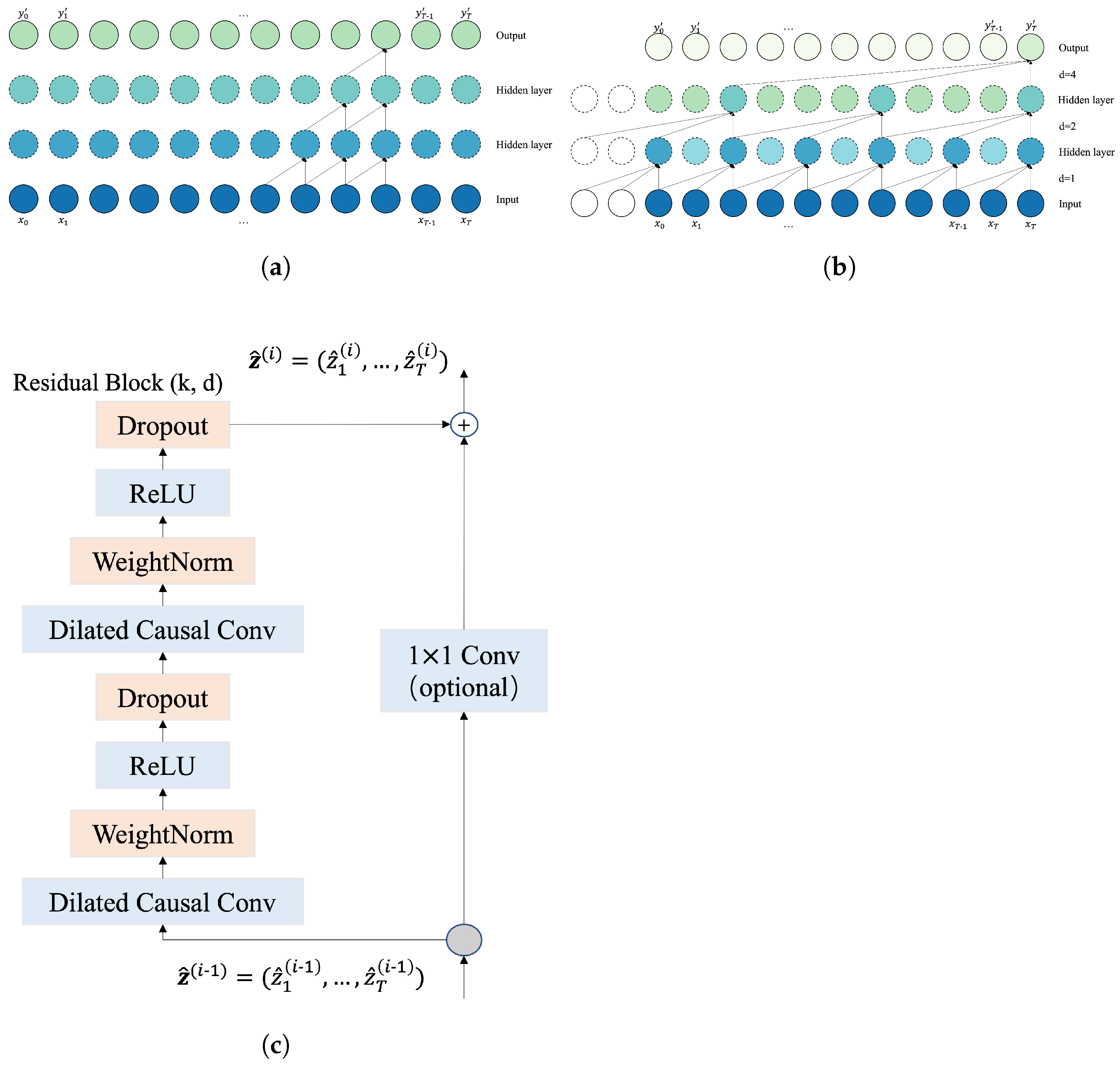
Deep learning-based sequence modeling methodologies have traditionally relied on recurrent neural networks (RNNs) for temporal dependency capture. Despite RNNs demonstrated capability in modeling long-range temporal relationships, their inherent sequential computation mechanism fundamentally restricts parallelization potential, consequently impeding training efficiency and inference scalability when processing large-scale datasets. To address these computational limitations, the temporal convolutional network (TCN) architecture was introduced as an innovative alternative [27], leveraging parallelizable convolutional operations to enhance computational efficiency. Through strategic stacking of convolutional layers with progressively expanding receptive fields, TCNs demonstrate enhanced capability in extracting localized temporal patterns while maintaining structural stability during gradient propagation. The architectural design of TCN incorporates three principal components: causal convolution, dilated convolution and residual connections [28], depicted in Figure 2.

2.4. The Proposed Model

The convolution operation of the standard TCN uses a fixed-weight kernel function for undifferentiated aggregation of features at all time steps, which makes it difficult to dynamically identify critical time nodes, such as sudden increases or decreases. Therefore, the attention mechanism [29] is introduced to assign different weights to each time step, which improves the attention to critical time steps. It also captures the remote dependencies of long sequences of PV data directly without increasing the depth of the convolutional layer.
In addition, fine-tuning multiple hyper-parameters based solely on intuition can be challenging. In order to find the optimal hyper-parameters when constructing neural network prediction models, Wang et al. [30] and Zhao et al. [31] introduced the butterfly optimization algorithm and particle swarm algorithm, respectively, to optimize the parameters of long short-term memory networks. To automate the selection of the optimal parameters of the neural network, we introduce Grey Wolf Optimizer (GWO) which improves model performance and convergence (Algorithm 1). GWO is inspired by the social hierarchy and group hunting behavior of grey wolves [32,33]. The optimization process simulates the roles and interactions among leader wolves (alpha), follower wolves (beta and delta), and regular wolves (omega). The optimization process is divided into three key parts: encircling, hunting, and attacking prey.
Algorithm 1 GWO Algorithm for Finding Optimal Hyperparameters
Require: loss_fun, dim=2, upper_bound, lower_bound, pop_size, max_iter
Ensure: best_params, best_fit
  1:
Initialization:
  2:
for  i = 0 to pop_size -1 do
  3:
      for  j = 0 to dim-1 do
  4:
             p o p u l a t i o n [ i ] [ j ] = l o w e r _ b o u n d [ j ] + r a n d o m ( )
( u p p e r _ b o u n d [ j ] l o w e r _ b o u n d [ j ] )
  5:
      end for
  6:
end for
  7:
Initialization the position of p a r a m 1 , p a r a m 2 , p a r a m 3 : p a r a m p o s 1 , p a r a m p o s 2 , p a r a m p o s 3 =(0,0), p a r a m l o s s 1 , p a r a m l o s s 2 , p a r a m l o s s 3 = i n f t y
  8:
for  i t e r = 0 to max_iter -1 do
  9:
       a = 2 i t e r ( 2 / m a x _ i t e r )
10:
      for  i = 0 to pop_size -1 do
11:
         Compute the training loss function for the model under each hyperparameter combination fitness=loss_fun
12:
         if fitness < p a r a m f i t n e s s 1  then
13:
                p a r a m l o s s 3 = p a r a m l o s s 2 , p a r a m p o s 3 = p a r a m p o s 2
14:
                p a r a m l o s s 2 = p a r a m l o s s 1 , p a r a m p o s 2 = p a r a m p o s 1
15:
                p a r a m l o s s 1 =fitness, p a r a m p o s 1 =population[i]
16:
         end if
17:
         if fitness < p a r a m l o s s 2  then
18:
                p a r a m l o s s 3 = p a r a m l o s s 2 , p a r a m p o s 3 = p a r a m p o s 2
19:
                p a r a m l o s s 2 =fitness, p a r a m p o s 2 =population[i]
20:
         end if
21:
         if fitness < p a r a m l o s s 3  then
22:
                p a r a m l o s s 3 =fitness, p a r a m p o s 3 =population[i]
23:
         end if
24:
      end for
25:
      for  i = 0 to pop_size -1 do
26:
         for  j = 0 to dim-1 do
27:
               Update the position of the hyperparameter population
28:
         end for
29:
         if population[i][j] < lower_bound[j] then
30:
               population[i][j] = lower_bound[j]
31:
         end if
32:
         if population[i][j] > lower_bound[j] then
33:
               population[i][j] = upper_bound[j]
34:
         end if
35:
      end for
36:
end for
37:
best_params= p a r a m p o s 1
38:
best_fit= p a r a m l o s s 1
39:
return best_params, best_fit
This improved hybrid neural architecture ITCN for enhanced short-term PV forecasting, integrating standard TCN, attention mechanisms, and GWO to simultaneously address prediction precision and operational stability. (1) TCN-based temporal feature extraction with dilated causal convolutions for long-range dependency modeling; (2) Attention-driven temporal weighting that prioritizes critical operational phases through adaptive context focusing; (3) Metaheuristic hyperparameter optimization by GWO, enabling systematic navigation of high-dimensional parameter spaces.
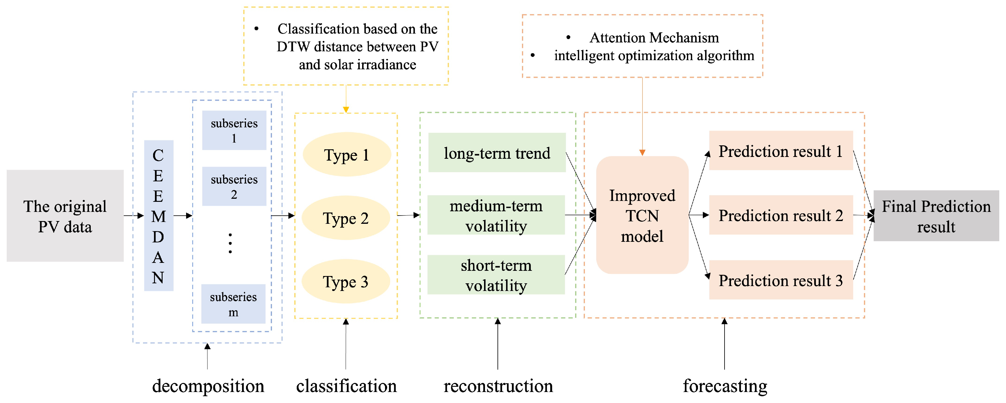
Finally, Figure 3 shows the overall framework of the proposed short-term PV prediction model.

3. Empirical Study

3.1. Data Description

This paper validates the proposed framework using anonymized operational data from two photovoltaic power stations in a region of China, designated as Dataset A and Dataset B, respectively. Dataset A comprises 66,859 records of actual irradiance and PV power data collected at 15 min intervals from 00:00 on 1 April 2016 to 23:45 on 30 April 2018. Dataset B covers corresponding data collected at 15 min intervals from 00:00 on 2 January 2017, to 23:45 on 30 April 2018, totaling 43,755 records. Each dataset is divided into training and test sets, with the first 70% used for training and the remaining 30% for testing.
Further analysis revealed that Dataset A should contain complete, continuous data samples from 1 April 2016, to 30 April 2018, totaling 96 × 760 = 72 , 960 data points, and Dataset B should contain complete, continuous data samples from 2 January 2017, to 30 April 2018, totaling 96 × 484 = 46 , 464 data points. However, due to potential equipment failures or transmission gaps, this dataset miss a negligible amount of data points. Given the sporadic nature of these missing points, forward-backward filling was utilized for imputation, which preserves the original data distribution without altering the statistical characteristics. Table 1 and Table 2 show the imputation details for datasets A and B.
Following the above processing, the final datasets A and B for model training and testing were obtained, retaining 33,308 and 43,073 valid data points, respectively. Table 3 presents the descriptive statistics for photovoltaic power in the two processed datasets.

3.2. Evaluation Criteria and Benchmark Models

A multi-metric evaluation matrix is implemented to rigorously assess predictive performance, including root mean square error, mean absolute error, symmetric mean absolute percentage error and coefficient of determination ( R 2 ). This metric ensemble systematically characterizes the error sensitivity, scale invariance, explanatory power and predictive efficiency of the proposed model.
This experiment establishes a baseline model from the following three aspects to comprehensively evaluate the performance of the proposed framework in short-term PV forecasting tasks. (1) To validate the superiority of CEEMDAN over other signal processing methods, EMD and VMD are selected for comparison, denoted as EMD-CR-TCN and VMD-CR-TCN models, respectively, where CR refers to the proposed improved data classification and reconstruction method. (2) To validate the effectiveness of the proposed data classification and reconstruction method, the CEEMDAN-TCN model is selected as the baseline where IMFs decomposed by the CEEMDAN method are directly fed into the TCN for prediction. (3) Convolutional neural networks (CNNs), long short-term memory (LSTM) networks, bidirectional LSTM networks, and bidirectional gated recurrent units (BiGRU) are selected for comparison to validate the improved TCN prediction model.

3.3. Experimental Design and Analysis

To achieve time series modeling of PV, this paper adopts a sliding window mechanism to convert the original time series data into a supervised learning format. Since the original data are recorded at intervals of 10 min, there are 144 time steps in a day ( 24 × 6 = 144 ). Therefore, we sets the window size to 144, using the historical observations of the previous 144 time steps as input features to predict the target variable, thus constructing the supervised training sample pairs. Compared to other forecasting methods, one-step prediction can reduce the problem of error accumulation and helps the model to learn the direct mapping relationship between input features and target variables more stably, making it suitable for high-frequency, short-term forecasting tasks. The specific experimental procedure of the model proposed in this paper will be illustrated in this section.
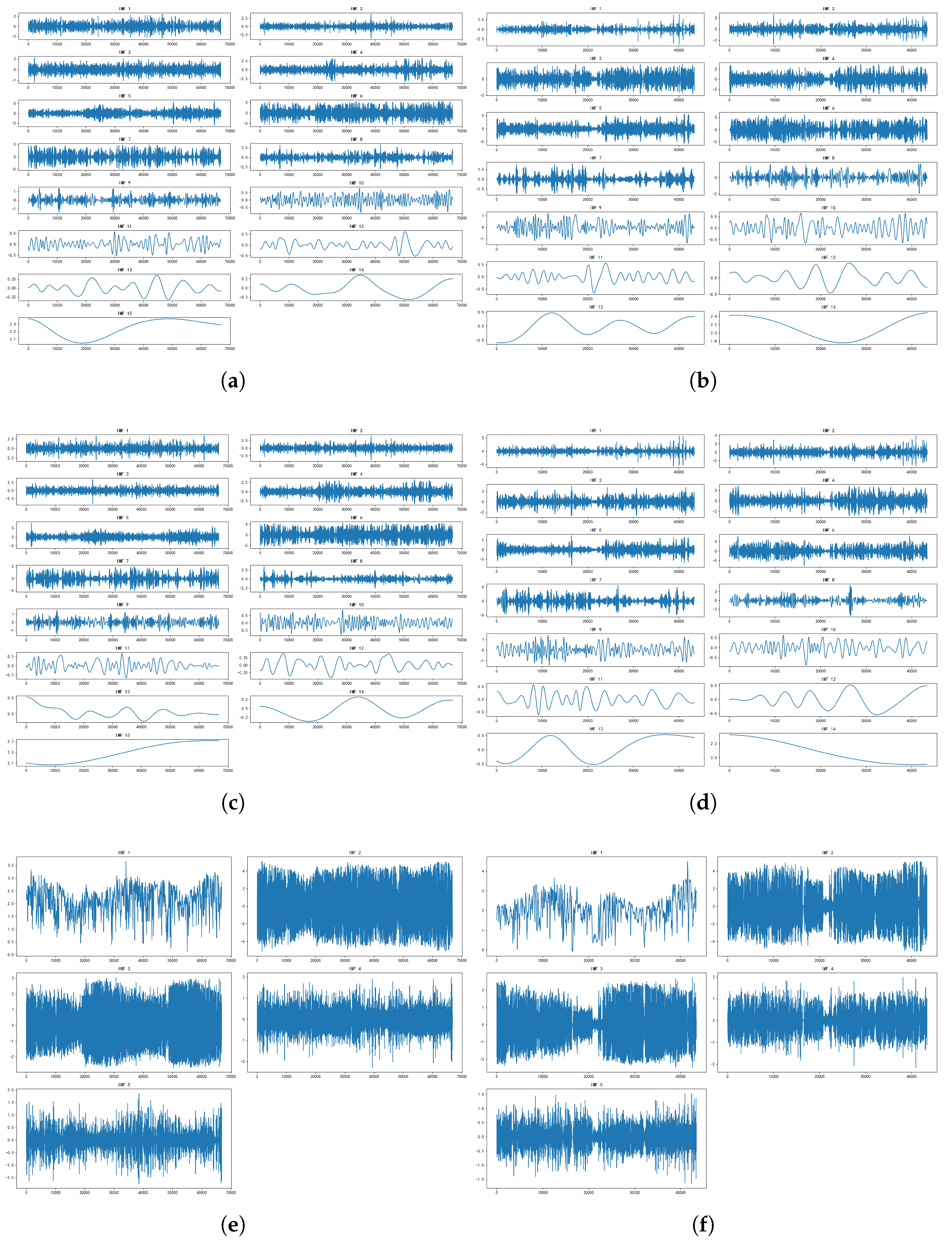
To demonstrate the superiority of the CEEMDAN decomposition method, we decomposed the original PV data, as shown in Figure 4. Both CEEMDAN and EMD decomposed Dataset A into 15 IMFs and Dataset B into 14 IMFs, whereas VMD decomposed two datasets into only 5 IMFs.
Then, the DTW distances between each IMF and the irradiance sequence were calculated, with results shown in Table 4. Using DTW distance as the classification criterion, IMFs were reconstructed into three new components. The classification results are presented in Table 5.
As shown in Table 6, comparing prediction models 1, 2, and 7 reveals the influence of different data decomposition methods on prediction results. For Dataset A, EMD yielded the poorest decomposition results for the PV data series. Compared to VMD and CEEMDAN, Model 7 achieved evaluation metrics of 0.45, 0.28, 101.59, and 0.98, respectively. Compared to Model 1, this resulted in a 22.4% reduction in RMSE, MAE decreased by 41.7%, SMAPE decreased by 38.3%, and R 2 increased by 0.01. For dataset B, the five metrics for models 1, 2, and 7 showed little difference, with the CEEMDAN method performing slightly better than the other two.
The prediction results of Models 3 and 7 demonstrate the importance of data classification and reconstruction. Classifying all IMFs into three components, long-term trend, medium-term fluctuation, and short-term fluctuation, before prediction enables the neural network model to better learn the variation patterns of each component. After incorporating classification and reconstruction, dataset A’s predictions showed a 0.23 reduction in RMSE, 0.34 in MAE, 18.32% in SMAPE, and a 0.03 increase in R 2 . Dataset B’s predictions exhibited a 19.7% decrease in RMSE, a 31.25% reduction in MAE, and a 0.02 increase in R 2 . This demonstrates that the “classification-reconstruction” operation effectively reduces prediction errors and enhances the model’s fitting capability.
To validate the performance advantages and applicability of TCN in real-time sequence data prediction tasks, this paper selected widely recognized neural network models within the field as benchmark models for comparative analysis. Comparisons of Models 4, 5, 6, and 7 demonstrate that the TCN model outperforms them across all four prediction evaluation metrics which demonstrates its unique advantages in regression prediction modeling, showcasing strong nonlinear feature extraction capabilities that better accommodate the regression modeling demands of complex data.
Based on Models 7 and 8, the proposed integration of attention mechanisms and intelligent optimization algorithms further enhances TCN performance and prediction accuracy. Setting the filter size optimization range to [32, 256] and kernel size range to [3, 9], the optimal hyperparameters obtained by intelligent optimization are shown in Table 7. For dataset A, the prediction RMSE, MAE, and SMAPE decreased by 64.4%, 21.4%, and 16.9%, respectively compared to Model 7, demonstrating significant reduction in prediction errors. For dataset B, all three prediction metrics also decreased, while the coefficient of determination R 2 increased. This indicates that the intelligent optimization algorithm can identify neural network model parameters that enhance prediction performance based on data characteristics, improving prediction accuracy while simultaneously strengthening the model’s generalization capability.
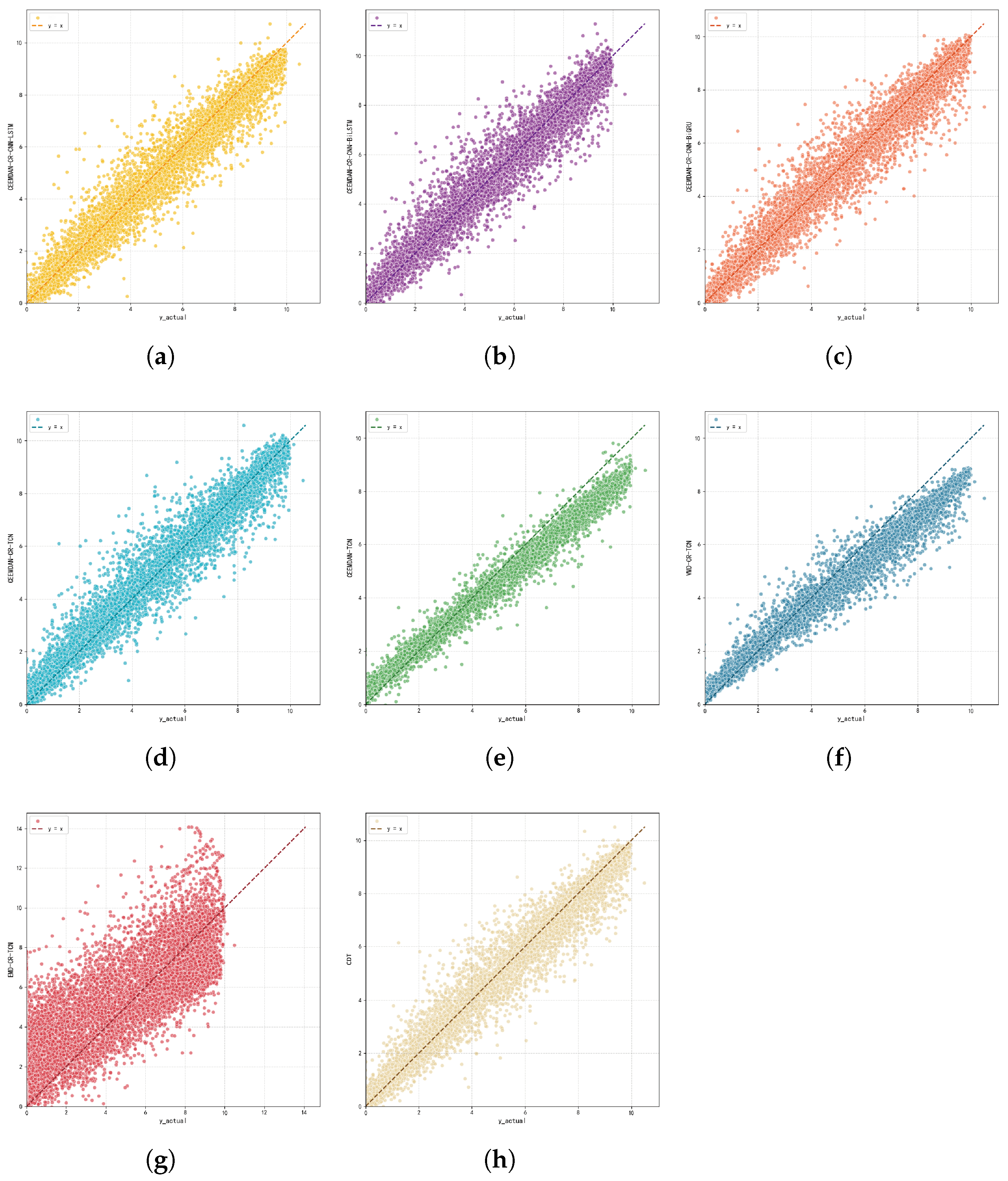
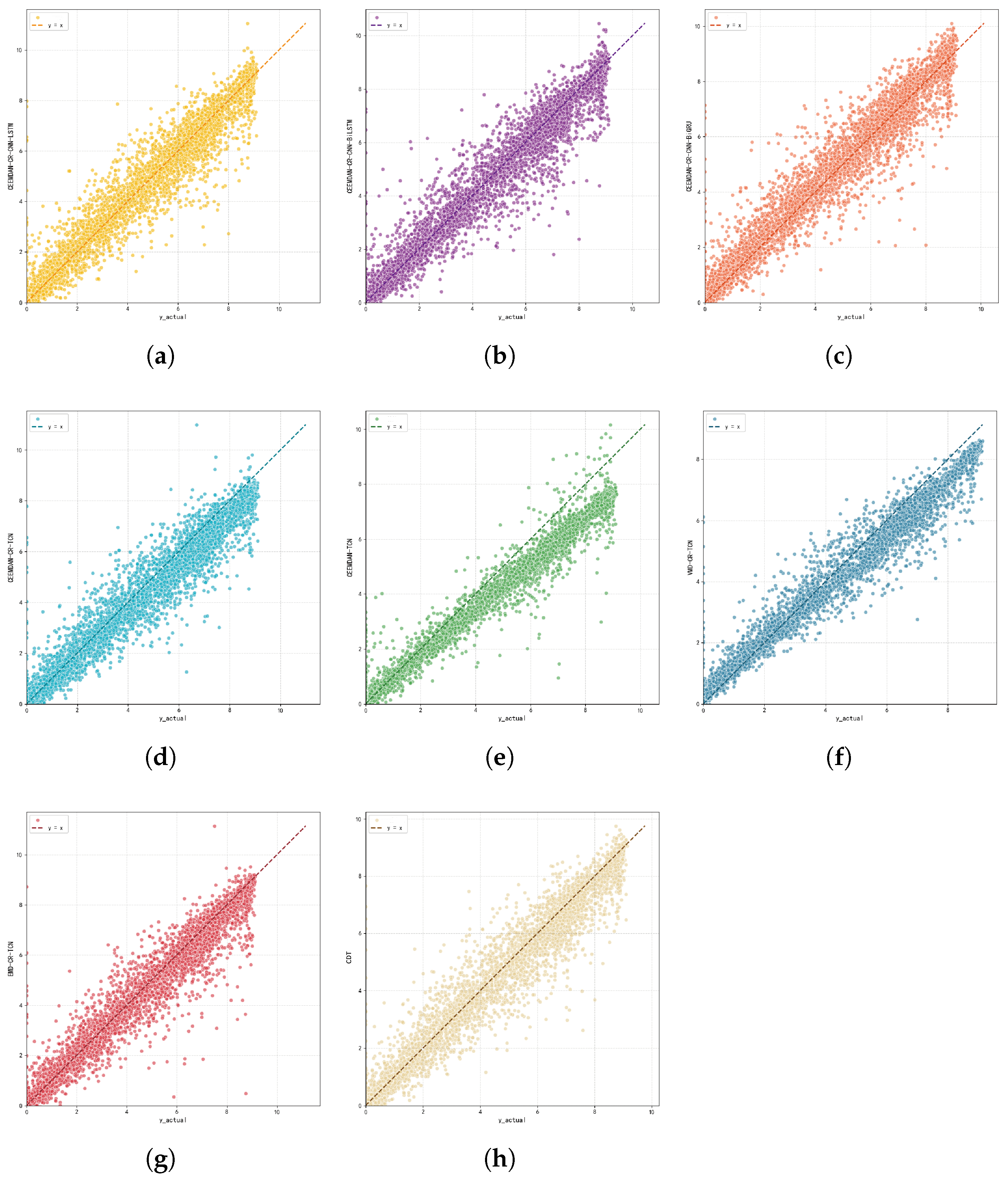
Figure 5 and Figure 6 display the scatter plots of predicted values and actual values for each model on Datasets A and B, providing a more intuitive representation of the prediction performance. The horizontal axis represents actual values, the vertical axis shows model predictions, and the dashed line denotes the y = x axis. The closer the scatter points cluster around this axis, the better the prediction performance. The figures reveal that Model 2 exhibits the most dispersed data points, indicating the poorest prediction performance for the dataset. Although Model 3 shows relatively concentrated scatter points, they deviate from the y = x axis, suggesting suboptimal prediction quality. Comparing all eight scatter plots, the CDT model demonstrates the most concentrated distribution of predicted values near the y = x axis.

3.4. Ablation Experiments

This section evaluates the contribution of the “data decomposition–classification–reconstruction” module, attention mechanism module and the intelligent optimization algorithm module to short-term PV forecasting capability by systematically removing them. To precisely assess the effect of these three components on prediction accuracy, we design ablation experiments to investigate their importance within the overall forecasting framework. Experimental results on dataset A and B are shown in Table 8 and Table 9.
CDT(-DCR): This model is trained and tested directly using original PV data, omitting the “data decomposition, classification, and reconstruction” steps to examine the importance and role of preprocessing before prediction.
CDT(-GWO): This model removes the module where intelligent optimization algorithms perform hyperparameter tuning on the neural network, instead using manually fixed hyperparameters to demonstrate the necessity of intelligent optimization algorithms for fine-tuning multiple parameters.
CDT(-Att): This model removes the attention mechanism to validate the importance of focusing on critical time steps when predicting long-sequence data such as PV power output.
CDT vs. CDT(-DCR): After removing the “data decomposition-classification-reconstruction” module and directly using original PV data as input for prediction with the improved TCN model, the performance of all four evaluation metrics was inferior to that of the CDT model for both Dataset A and Dataset B. This indicates the original data contained more noise and irrelevant information, making it difficult for the model to learn effective prediction patterns. The “Data Decomposition–Classification–Reconstruction” module classifies and reconstructs multiple intrinsic mode functions into three components with practical physical significance. This mechanism highlights key features while mitigating non-stationarity issues, enabling the model to capture patterns more effectively.
CDT vs. CDT(-GWO): Setting the number of filters in the improved TCN prediction model to 64 and the kernel size to 3. As shown in the table, fixed hyperparameters may fail to adequately capture complex patterns across different frequency data. Intelligent optimization algorithms effectively identify hyperparameter configurations better suited to specific datasets by systematically exploring the parameter space.
CDT vs. CDT(-Att): On dataset A, all metrics of CDT(-Att) underperformed those of CDT. On dataset B, both models maintain RMSE and MAE values at 0.46 and 0.25, respectively, while achieving R 2 of 0.98. This outcome demonstrates that the backbone network of CDT possesses feature extraction and nonlinear mapping capabilities. Without relying on attention mechanisms, the model can accurately capture the global evolutionary trends within data sequences. After introducing the attention mechanism, SMAPE decreased from 119.32 to 118.30. This optimization indicates that by assigning higher weights to critical time steps in the historical sequence, the mechanism effectively mitigates prediction lag or over-smoothing issues when handling local sudden changes, extreme values, or low-value intervals. Consequently, it enhances the relative prediction accuracy of local features.
In addition, to better assess the model’s robustness and practical applicability, supplementary experimental validation is conducted. We generated a 30 min interval subset from Dataset A and a subset from Dataset B through downsampling and formed two new Dataset C and D. We re-evaluated the capabilities of the proposed model at this new resolution. The DTW distance between each IMF and corresponding solar irradiance sequence are listed in Table 10. According to the K-Means clustering algorithm, for dataset C, the long-term trend comprises IMF 3 and 5, and the medium-term fluctuation comprises IMF 1, 2, and 4, others are assigned to short-term fluctuation. For dataset D, the long-term trend consists of IMF 2, 3, and 4, the medium-term fluctuation consists of 1, 6, 7, 8, 9, 10 and 11, and IMF 12 and 13 are classified as short-term fluctuations.
As shown in Table 11, for both datasets, after downsampling to 30 min intervals, all error metrics of the CDT model (RMSE, MAE, SMAPE) increased, and the coefficient of determination R 2 decreased. Downsampling from 15 to 30 min resulted in severe loss of high-frequency dynamic features in the sequence. These high-frequency features serve as the critical information source for the attention mechanism to perform precise weight allocation. The smoothing of the feature space instead led to information loss. Furthermore, the reduction in temporal resolution caused the available training sample size to decrease by 50%, limiting the thorough optimization of the deep network parameter space.

4. Conclusions

Social development requires a continuous supply of energy from the power grid, and renewable energy is being developed and utilized in large quantities to build a low-carbon and environmentally friendly power system. The unstable characteristics of PV reduce the robustness of power system operation, so it is necessary to improve the accuracy and credibility of prediction. For this reason, this paper proposes a data-driven CEEMDAN and DTW-based TCN short-term PV power prediction framework (CDT). After data decomposition, the DTW distance between the PV trend subseries (PVTS) and the contemporaneous solar irradiance is regarded as a criterion. The subsequences were then categorized to remove the detrimental effects of noise and reduce the computational complexity. The PVTSs are reconstructed and denoted as long-term trend component, medium-term fluctuation component, and short-term volatility component. Finally, an improved temporal convolutional network is built to forecast the reconstructed components. In the empirical analysis section, the 15 min interval power data in two datasets are extracted for prediction. In order to verify the prediction accuracy of the proposed model, seven benchmark models are designed. From the results, it can be seen that our CDT model outperforms all the benchmark models, which indicates that the classification and reconstruction stage can help to extract the complex features of the PV series while reducing the data dimension. Despite the promising results, this study is currently limited to specific geographical regions due to the commercial confidentiality of PV plant data. Future work will focus on acquiring datasets from diverse climate zones to further validate the cross-regional robustness of the proposed framework.

Author Contributions

Methodology, J.Z.; Data curation, Y.S.; Writing—original draft, Y.S.; Writing—review & editing, G.W. and J.Z.; Funding acquisition, G.W. All authors have read and agreed to the published version of the manuscript.

Funding

This research was funded by National Natural Science Foundation of China (No. 72472147) and Xinjiang Production and Construction Corps (No. 2024AB061).

Institutional Review Board Statement

Not applicable.

Informed Consent Statement

Not applicable.

Data Availability Statement

The data can be made available from the corresponding author upon request.

Conflicts of Interest

The authors declare no conflicts of interest.

References

  1. Xiao, Y.; Xiao, G.; Li, J. Photovoltaic-energy storage systems empowered: Low-carbon and economic scheduling for electric buses. Transp. Res. Part D Transp. Environ. 2026, 150, 105082. [Google Scholar] [CrossRef]
  2. Zhang, K.; Zhang, J.; Xu, P.D.; Gao, T.; Gao, D.W. Explainable AI in Deep Reinforcement Learning Models for Power System Emergency Control. IEEE Trans. Comput. Soc. Syst. 2021, 9, 419–427. [Google Scholar] [CrossRef]
  3. Di Leo, P.; Ciocia, A.; Malgaroli, G.; Spertino, F. Advancements and Challenges in Photovoltaic Power Forecasting: A Comprehensive Review. Energies 2025, 18, 2108. [Google Scholar] [CrossRef]
  4. Wang, R.; Liu, X.; Chang, Y.; Liu, D.; Yao, H. Short-Term Photovoltaic System Output Power Prediction Based on Integrated Deep Learning Algorithms in the Clean Energy Sector. Int. J. E-Collab. (IJeC) 2024, 20, 1–15. [Google Scholar] [CrossRef]
  5. Cican, G.; Buturache, A.N.; Silivestru, V. Predicting photovoltaic energy production using neural networks: Renewable integration in Romania. Processes 2025, 13, 2219. [Google Scholar] [CrossRef]
  6. Zhao, M.; Li, S.; Chen, H.; Ling, M.; Chang, H. Distributed solar photovoltaic power prediction algorithm based on deep neural network. J. Eng. Res. 2024, 13, 3352–3359. [Google Scholar] [CrossRef]
  7. Ouyang, J.; Chu, L.; Chen, X.; Zhao, Y.; Zhu, X.; Liu, T. A K-means cluster division of regional photovoltaic power stations considering the consistency of photovoltaic output. Sustain. Energy Grids Netw. 2024, 40, 101573. [Google Scholar] [CrossRef]
  8. Zhang, R.; Pang, C.; Zhu, X.; Gao, F.; Jiang, P. A Short-term photovoltaic power prediction method based on the nearest clear sky day decomposition and temporal convolutional network. Electr. Eng. 2025, 107, 11075–11086. [Google Scholar] [CrossRef]
  9. Aman, R.; Rizwan, M.; Kumar, A. A novel hybrid intelligent approach for solar photovoltaic power prediction considering UV index and cloud cover. Electr. Eng. 2025, 107, 1203–1224. [Google Scholar] [CrossRef]
  10. Yang, M.; Guo, Z.; Wang, D.; Wang, B.; Wang, Z.; Huang, T. Short-term photovoltaic power forecasting method considering historical information reuse and numerical weather forecasting. Renew. Energy 2025, 256, 123933. [Google Scholar] [CrossRef]
  11. Sun, F.; Li, L.; Bian, D.; Bian, W.; Wang, Q.; Wang, S. Photovoltaic power prediction based on multi-scale photovoltaic power fluctuation characteristics and multi-channel LSTM prediction models. Renew. Energy 2025, 246, 122866. [Google Scholar] [CrossRef]
  12. Wang, X.; Hu, M.; Luo, X.; Guan, X. Spatio-temporal photovolatic power forecasting via Bayesian-optimized dynamic graph convolutional networks with temporal convolutional networks. J. Clean. Prod. 2026, 542, 147641. [Google Scholar] [CrossRef]
  13. Zhuang, W.; Li, Z.; Wang, Y.; Xi, Q.; Xia, M. GCN–informer: A novel framework for mid-term photovoltaic power forecasting. Appl. Sci. 2024, 14, 2181. [Google Scholar] [CrossRef]
  14. Guan, X.; Han, X.; Wang, J.; Wang, T. A novel short-term prediction method for distributed photovoltaic power generation considering extreme weather. Eng. Appl. Artif. Intell. 2025, 162, 112540. [Google Scholar] [CrossRef]
  15. Chao, M.; Yu, J.; Cao, W.; Wang, M.; Zhou, M. An improved hybrid neural network algorithm for predicting photovoltaic output power: Considering the seasonal output characteristics of solar energy. J. Renew. Sustain. Energy 2025, 17, 026101. [Google Scholar] [CrossRef]
  16. Peng, L.L.; Ge, Q.Y.; Fan, G.F.; Hong, W.C. Short-term photovoltaic power prediction based on volatility analysis and uncertainty measurement. J. Renew. Sustain. Energy 2025, 17, 053505. [Google Scholar] [CrossRef]
  17. Zhou, D.; Liu, Y.; Wang, X.; Wang, F.; Jia, Y. Combined ultra-short-term photovoltaic power prediction based on CEEMDAN decomposition and RIME optimized AM-TCN-BiLSTM. Energy 2025, 318, 134847. [Google Scholar] [CrossRef]
  18. Yu, J.; Liang, G.; Wang, L.; He, H.; Liu, Y.; Liu, Q.; Cui, X.; Wang, H. Short-term power prediction of photovoltaic power stations based on Kepler optimization algorithm and VMD-CNN-LSTM model. PLoS ONE 2025, 20, e0329821. [Google Scholar] [CrossRef]
  19. Liu, M.; Wang, X.; Zhong, Z. Ultra-short-term photovoltaic power prediction based on BiLSTM with wavelet decomposition and dual attention mechanism. Electronics 2025, 14, 306. [Google Scholar] [CrossRef]
  20. Wu, Y.; Pan, X.; Yang, J. VMD-Informer-DCC for photovoltaic power prediction. IEICE Trans. Commun. 2024, 107, 487–494. [Google Scholar] [CrossRef]
  21. Wu, S.; Guo, H.; Zhang, X.; Wang, F. Short-Term Photovoltaic Power Prediction Based on CEEMDAN and Hybrid Neural Networks. IEEE J. Photovoltaics 2024, 14, 960–969. [Google Scholar] [CrossRef]

  22. Zhan, Y.; Wang, X.; Xu, Y.; Li, W. A Hybrid TCN-LSTM-Attention Framework for Multi-Scenario Short-Term Photovoltaic Power Forecasting Incorporating Physics-Informed Neural Network Strategy. Energy 2026, 344, 139968. [Google Scholar] [CrossRef]
  23. Li, B.; Wang, H.; Zhang, J. Short-term power forecasting of photovoltaic generation based on CFOA-CNN-BiLSTM-Attention. Electr. Eng. 2025, 107, 10335–10347. [Google Scholar] [CrossRef]
  24. Souhe, F.G.Y.; Mbey, C.F.; Kakeu, V.J.F.; Meyo, A.E.; Boum, A.T. Optimized forecasting of photovoltaic power generation using hybrid deep learning model based on GRU and SVM. Electr. Eng. 2024, 106, 7879–7898. [Google Scholar] [CrossRef]
  25. Torres, M.E.; Colominas, M.A.; Schlotthauer, G.; Flandrin, P. A complete ensemble empirical mode decomposition with adaptive noise. In Proceedings of the 2011 IEEE International Conference on Acoustics, Speech and Signal Processing (ICASSP), 22–27 May 2011, Prague, Czech Republic; IEEE: New York, NY, USA, 2011; pp. 4144–4147. [Google Scholar] [CrossRef]
  26. Sakoe, H.; Chiba, S. Dynamic programming algorithm optimization for spoken word recognition. IEEE Trans. Acoust. Speech Signal Process. 1978, 26, 43–49. [Google Scholar] [CrossRef]
  27. Bai, S.; Kolter, J.Z.; Koltun, V. An empirical evaluation of generic convolutional and recurrent networks for sequence modeling. arXiv 2018, arXiv:1803.01271. [Google Scholar] [CrossRef]
  28. Xiao, Y.; Wu, S.; He, C.; Hu, Y.; Yi, M. An effective hybrid wind power forecasting model based on “decomposition-reconstruction-ensemble” strategy and wind resource matching. Sustain. Energy Grids Netw. 2024, 38, 101293. [Google Scholar] [CrossRef]
  29. Vaswani, A.; Shazeer, N.; Parmar, N.; Uszkoreit, J.; Jones, L.; Gomez, A.N.; Kaiser, Ł.; Polosukhin, I. Attention is all you need. Adv. Neural Inf. Process. Syst. 2017, 30, 5998–6008. [Google Scholar] [CrossRef]
  30. Wang, Y.; Zhao, K.; Hao, Y.; Yao, Y. Short-term wind power prediction using a novel model based on butterfly optimization algorithm-variational mode decomposition-long short-term memory. Appl. Energy 2024, 366, 123313. [Google Scholar] [CrossRef]
  31. Zhao, Y.; Li, L.; Guo, Y.; Shi, B.; Sun, H. Short-term wind power prediction based on combined long short-term memory. IET Gener. Transm. Distrib. 2024, 18, 931–940. [Google Scholar] [CrossRef]
  32. Mirjalili, S.; Mirjalili, S.M.; Lewis, A. Grey wolf optimizer. Adv. Eng. Softw. 2014, 69, 46–61. [Google Scholar] [CrossRef]
  33. Liu, J.; Hou, Z.; Yin, T. Short-term power load forecast using OOA optimized bidirectional long short-term memory network with spectral attention for the frequency domain. Energy Rep. 2024, 12, 4891–4908. [Google Scholar] [CrossRef]
Figure 1. Workflow of CEEMDAN.
Sustainability 18 02719 g001
Figure 2. Structure of TCN. (a) Structure of Causal Convolution; (b) Structure of Causal Convolutiondilated Convolution; (c) Structure of Residual Block.
Sustainability 18 02719 g002
Figure 3. The Framework of CDT Model.
Sustainability 18 02719 g003
Figure 4. Decomposition results of Dataset A and B. (a,c,e) CEEMDAN, EMD, VMD Decomposition Results of Dataset A; (b,d,f) CEEMDAN, EMD, VMD Decomposition Results of Dataset B.
Sustainability 18 02719 g004
Figure 5. Comparison of Prediction Model Results with Actual Values for Dataset A: (a) CEEMDAN-CR-CNN-LSTM, (b) CEEMDAN-CR-CNN-BILSTM, (c) CEEMDAN-CR-CNN-BIGRU, (d) CEEMDAN-CR-TCN, (e) CEEMDAN-TCN, (f) VMD-CR-TCN, (g) EMD-CR-TCN, (h) CDT.
Sustainability 18 02719 g005
Figure 6. Comparison of Prediction Model Results with Actual Values for Dataset B: (a) CEEMDAN-CR-CNN-LSTM, (b) CEEMDAN-CR-CNN-BILSTM, (c) CEEMDAN-CR-CNN-BIGRU, (d) CEEMDAN-CR-TCN, (e) CEEMDAN-TCN, (f) VMD-CR-TCN, (g) EMD-CR-TCN, (h) CDT.
Sustainability 18 02719 g006
Table 1. Data Imputation and Explanation for Dataset A.
TimeSolar IrradiancePhotovoltaic PowerExplanation
2017-01-01 00:0000Nighttime (zero irradiance)
2017-01-09 09:1568.380.72Mean of three preceding and succeeding measurements
2017-04-01 00:000−0.07Nighttime (zero irradiance)
2017-05-25 20:000−0.022Nighttime (zero irradiance)
2017-05-25 20:150−0.022Nighttime (zero irradiance)
2017-05-26 19:1588.880.52Mean of three preceding and succeeding measurements
2017-06-16 11:30843.437.92Mean of three preceding and succeeding measurements
2017-08-04 19:4547.720.25Mean of three preceding and succeeding measurements
2017-08-22 18:1592.140.89Mean of three preceding and succeeding measurements
2017-12-01 00:0000Nighttime (zero irradiance)
Table 2. Data Imputation and Explanation for Dataset B.
TimeSolar IrradiancePhotovoltaic PowerExplanation
2017-02-27 18:459.720.022Mean of measurements recorded at the same time over
the preceding and following three days
2017-03-06 10:00380.726.64Mean of three preceding and succeeding measurements
2017-04-07 10:45609.063.81Mean of three preceding and succeeding measurements
2017-04-07 11:00635.683.87Mean of three preceding and succeeding measurements
2017-05-26 10:30639.526.50Mean of three preceding and succeeding measurements
2017-05-26 13:001064.928.06Mean of three preceding and succeeding measurements
2017-06-27 09:00420.110Mean of three preceding measurements
2017-06-27 09:15435.50Mean of three preceding measurements
2017-06-27 09:30439.780Mean of three preceding measurements
2017-06-27 09:45431.800Mean of three preceding measurements
2017-06-28 10:30716.610Mean of three preceding and succeeding measurements
2017-08-05 15:00755.074.73Mean of three preceding measurements
2017-08-05 15:15779.454.73Mean of three preceding measurements
2017-08-05 15:30779.174.67Mean of three preceding and succeeding measurements
2018-01-01 00:0000Nighttime (zero irradiance)
Table 3. Descriptive Statistics for the Photovoltaic Power of Processed Dataset A and B.
Sample SizeMeanMedianStandard DeviationMaximum ValueQuartiles
Dataset ASpring4.163.883.019.553.88
Summer3.683.332.849.533.33
Autumn4.164.22.789.544.2
Winter4.835.392.969.555.39
Dataset BSpring2.30.033.048.850.03
Summer1.910.172.428.830.17
Autumn1.7102.738.810
Winter1.8402.778.490
Table 4. DTW distances between IMFs and Solar Irradiance for Dataset A and B.
Dataset ADataset B
CEEMDAN EMD VMD CEEMDAN EMD VMD
DTW distance 153.0354.9264.9745.0046.2044.62
DTW distance 264.1263.0635.7542.4840.7132.87
DTW distance 354.1767.2033.8334.7138.2830.80
DTW distance 458.7260.0061.7537.5337.4941.91
DTW distance 562.8955.1454.2441.8745.2040.61
DTW distance 651.1848.00-33.0140.56-
DTW distance 751.9855.32-42.3541.01-
DTW distance 863.3766.05-46.9847.83-
DTW distance 965.6265.07-47.1246.84-
DTW distance 1065.5065.46-47.7351.56-
DTW distance 1166.5467.02-51.6049.30-
DTW distance 1267.3367.60-50.6951.05-
DTW distance 1367.5767.99-49.1749.94-
DTW distance 1468.0968.18-64.8370.32-
DTW distance 1569.6369.82----
Table 5. Results of the classification of IMFs for dataset A and B.
DatasetShort-Term FluctuationMedium-Term FluctuationLong-Term Trend
CEEMDANA2, 5, 8–1541, 3, 6, 7
B141, 2, 5, 7–133, 4, 6
EMDA2, 3, 8–151, 4, 5, 76
B141, 5, 8–132, 3, 4, 6, 7
VMDA1, 452, 3
B14, 52, 3
Table 6. Evaluations of Different Models for Dataset A and B.
Dataset ADataset B
RMSE MAE SMAPE R 2 RMSE MAE SMAPE R 2
VMD-CR-TCN0.580.48164.730.970.480.34168.130.97
EMD-CR-TCN3.292.74145.710.940.490.26174.590.97
CEEMDAN-TCN0.680.62119.910.950.660.48167.760.95
CEEMDAN-CR-CNN-LSTM0.420.23154.310.980.470.23174.430.97
CEEMDAN-CR-CNN-BiLSTM0.440.25163.790.980.490.25174.540.97
CEEMDAN-CR-CNN-BiGRU0.410.23156.680.980.500.30170.130.97
CEEMDAN-CR-TCN0.450.28101.590.980.530.33171.760.97
CDT0.160.2284.460.990.460.25118.300.98
Table 7. Optimal Hyperparameters for Each Component Prediction Model.
DatasetComponentsFilter SizeKernel Size
Along-term trend325
medium-term fluctuation645
short-term fluctuation327
Blong-term trend325
medium-term fluctuation323
short-term fluctuation647
Table 8. Evaluations of Ablation Experiments for Dataset A.
RMSEMAESMAPE R 2
CDT(-DCR)1.330.67130.780.82
CDT(-GWO)fil = 64, ks = 31.641.34160.730.73
CDT(-Att)0.410.2398.030.98
CDT0.160.2284.460.99
Table 9. Evaluations of Ablation Experiments for Dataset B.
RMSEMAESMAPE R 2
CDT(-DCR)1.470.82131.600.77
CDT(-GWO)fil = 64, ks = 31.401.07167.450.79
CDT(-Att)0.460.25119.320.98
CDT0.460.25118.300.98
Table 10. DTW distance between IMFs and Solar Irradiance for Dataset C and D.
DTW DistanceDataset CDataset D
140.3031.31
238.3528.92
331.7625.16
439.8927.96
534.0724.97
645.4233.15
745.0232.20
847.0533.36
946.3635.11
1047.5436.70
1148.2234.06
1248.5453.75
1348.5253.10
1449.59-
Table 11. Evaluations of CDT for Dataset C and D.
RMSEMAESMAPE R 2
Dataset A
(15 min interval)
0.160.2284.460.99
Dataset C
(30 min interval)
2.471.97137.920.39
Dataset B
(15 min interval)
0.450.25118.300.98
Dataset D
(30 min interval)
1.170.92128.480.85
Disclaimer/Publisher’s Note: The statements, opinions and data contained in all publications are solely those of the individual author(s) and contributor(s) and not of MDPI and/or the editor(s). MDPI and/or the editor(s) disclaim responsibility for any injury to people or property resulting from any ideas, methods, instructions or products referred to in the content.