Article

Analysis and Prediction Evaluation of Provincial Carbon Emissions Under Multi-Model Fusion

1
School of Transportation Engineering, Shandong Jianzhu University, Jinan 250101, China
2
Management Engineering, Zhengzhou University of Aeronautics, Zhengzhou 450001, China
3
Shandong Taihe Urban Construction Development Co., Ltd., Zibo 256410, China
*
Authors to whom correspondence should be addressed.
Sustainability 2026, 18(5), 2545; https://doi.org/10.3390/su18052545
Submission received: 25 January 2026 / Revised: 16 February 2026 / Accepted: 3 March 2026 / Published: 5 March 2026

Abstract

Against the backdrop of sustainable development and global climate governance, this study focuses on the evaluation and trend prediction of provincial carbon emission efficiency and constructs a multi-model integrated analytical framework featuring “data preprocessing—efficiency decomposition—dynamic forecasting—policy deduction”. First, economic, energy consumption and carbon emission data for 30 provinces in China from 2009 to 2019 are collected. Data cleaning is performed through outlier identification and Lagrange interpolation, and a cross-regionally comparable quantification system is established based on a unified carbon emission standard, laying a foundation for subsequent analysis. Second, data envelopment analysis (DEA) is adopted to decompose carbon emission efficiency. It is found that approximately 23% of provinces lie on the technical efficiency frontier, with the average variance share of technical inefficiency being 0.62; 6% of provinces have the potential for scale expansion; and 10% suffer from diseconomies of scale, reflecting significant structural efficiency losses in regions concentrated with high-carbon industries. Third, the long short-term memory (LSTM) neural network is employed for dynamic forecasting and scenario simulation of carbon emissions by 2025. The model’s prediction error in 2019 is controlled within 8.7%. Simulation results show that when the share of clean energy rises to 35%, China’s national carbon emission growth rate can be reduced to 1.2% by 2025. However, multi-scenario sensitivity analysis indicates that the achievement of this target highly depends on policy enforcement intensity and power grid accommodation capacity. In addition, stochastic frontier analysis (SFA) reveals the heterogeneous contributions of different energy types to economic and social outputs. The consumption elasticities of electricity, liquefied petroleum gas and gasoline are significantly positive, whereas the negative elasticities of oil, fuel oil and coal deeply reflect the low energy utilization efficiency and rigid lock-in of high-carbon industries in some regions. Finally, combined with efficiency evaluation, trend prediction and mechanism analysis, differentiated emission reduction strategies are proposed for technologically backward provinces, scale-imbalanced provinces and clean energy base provinces, forming a complete closed loop from “efficiency diagnosis” to “future deduction” and then to “policy feedback”. This study breaks through the limitations of a single model. Through the coupling of parametric and non-parametric methods, as well as the integration of dynamic forecasting and scenario simulation, it effectively addresses issues such as data heterogeneity. It provides scientific support for local governments to formulate emission reduction policies and optimize energy structures, establishes a methodological foundation for industrial efficiency analysis and international carbon responsibility allocation research, and helps to promote regional clean, low-carbon, and sustainable development.

1. Introduction

Against the background of the global active response to climate change and in-depth advancement of the “dual carbon” goals, carbon emissions have become the focus of international attention. As the world’s largest energy consumer and carbon emitter, China is confronted with the enormous pressure of carbon emission reduction while promoting high-quality economic development. From a global perspective, carbon emissions are highly concentrated in a few major coal-consuming countries. According to statistics from the International Energy Agency (IEA) and relevant sources, the top five countries in terms of global hard coal and lignite mining and combustion volumes are China, India, the United States, Australia, and Indonesia, respectively. These countries have coal-dominated energy structures, and their carbon emission trajectories exert a decisive impact on the achievement of global climate goals. Therefore, how to scientifically evaluate and effectively reduce carbon emissions in regions dependent on high-carbon energy has become a major issue that urgently needs to be addressed for global sustainable development.
Although scholars at home and abroad have achieved fruitful results in the field of carbon emission research, there are still research gaps that urgently need to be filled. First, at the methodological level, most existing studies adopt a single model (such as only data envelopment analysis (DEA) or only stochastic frontier analysis (SFA)) for analysis, in which it is difficult to simultaneously take into account the non-parametric flexibility of efficiency evaluation and the statistical inference capability of parametric methods, resulting in an insufficiently comprehensive and in-depth measurement of carbon emission efficiency. Second, from the research perspective, the existing literature rarely systematically couples static efficiency decomposition with dynamic trend prediction and scenario simulation, making it difficult to form a complete closed loop from “current situation diagnosis” to “future deduction” and then to “policy formulation”. In addition, regarding the phenomenon of “regional imbalance and efficiency differentiation” among various provinces in China, which is caused by differences in resource endowments, industrial structures and development stages, the existing studies lack a unified analytical framework that can effectively handle data heterogeneity and realize cross-regional comparable quantification. Integrating the concept of sustainable development into carbon emission efficiency research holds significant theoretical value and practical implications for promoting regional coordinated development and green low-carbon transition.
To fill the above gaps, this study will address the following core research questions: First, how can we integrate the parametric method (stochastic frontier analysis, SFA) and the non-parametric method (data envelopment analysis, DEA) to accurately decompose and evaluate the carbon emission technical efficiency and scale efficiency of 30 provinces in China? Second, how can we use the long short-term memory (LSTM) neural network to capture the temporal dependence characteristics of carbon emissions and realize the dynamic prediction of provincial carbon emission trends? Third, combined with efficiency analysis and scenario simulation, how should different provinces formulate differentiated emission reduction paths and policy combinations to coordinately achieve high-quality regional economic development and the “dual carbon” goals, and thereby promote sustainable development in China and other global high-carbon-dependent regions? Through in-depth exploration of these issues, this study aims to provide a more scientific and accurate decision-making basis for emission reduction in China and global high-carbon-dependent regions.

2. Literature Review

2.1. Overview of the Retrieval Process

To systematically grasp the research frontiers and methodological evolution in the field of provincial carbon emissions, this study carried out standardized literature retrieval covering three major databases—China National Knowledge Infrastructure (CNKI), Web of Science Core Collection, and ScienceDirect—with a time span from 2000 to 2025 to integrate both classic theories and cutting-edge progress; the search terms adopted were “provincial carbon emissions”, “carbon emission efficiency”, “data envelopment analysis”, “stochastic frontier analysis”, “LSTM neural network”, and “dual carbon goals”, and finally more than 40 core literature articles highly relevant to the research theme were screened. These literature articles cover the mainstream directions of current provincial carbon emission research, including frontier fields such as the DEA-SBM model, three-stage SBM-undesirable model coupled with LSTM, multi-directional efficiency analysis, machine learning prediction, scenario simulation and policy deduction, providing theoretical support and methodological references for this study to construct a multi-model integration framework of “data preprocessing–efficiency decomposition–dynamic prediction–policy deduction”. In the process of data analysis and modeling, the following software tools were used: data preprocessing and descriptive statistical analysis were completed with Excel 2021 and SPSS 26.0, data envelopment analysis models were solved by DEAP 2.1, parameter estimation of stochastic frontier analysis was realized via Frontier 4.1, the construction, training and prediction of the LSTM neural network were based on Python 3.9 using TensorFlow 2.0 and Keras framework, and chart plotting was performed using Origin 2021 and the Matplotlib toolkit version 3.5.1.

2.2. Domestic Literature Review

Domestic scholars have achieved fruitful results in the field of provincial carbon emission research. In terms of carbon emission status analysis, Chen Gang [1] applied the generalized data envelopment analysis method to evaluate the carbon emission efficiency of the construction industry in his work Evaluation of Carbon Emission Efficiency in the Construction Industry Using Generalized Data Envelopment Analysis, providing a methodological reference for carbon emission research in specific industries within provinces. Due to differences in economic development levels, industrial structures, and energy consumption structures, carbon emission characteristics vary significantly among provinces. Provinces with developed economies and a high proportion of industry, such as Guangdong and Jiangsu, tend to have high total carbon emissions, while provinces dominated by agriculture or the service industry have relatively low carbon emissions.
Regarding the path to achieve provincial dual carbon goals, Zhang Chenyue [2] discussed carbon emission calculation and emission reduction paths in their work Study on Carbon Emission Calculation of Shandong Jianzhu University. Domestic scholars generally believe that optimizing energy structure, improving energy utilization efficiency, developing low-carbon technologies, and strengthening carbon emission management are effective ways to achieve the goals. Some provinces have taken active actions, vigorously developing renewable energy such as solar and wind energy, and gradually reducing dependence on fossil energy to reduce carbon emissions.

2.3. Foreign Literature Review

Foreign scholars have formed a rich research system in the field of provincial-level carbon emission studies, and research methodologies have demonstrated a clear evolutionary path from single models to multi-model integration and from static evaluation to dynamic prediction.
In terms of carbon emission efficiency evaluation, data envelopment analysis and its derivative models have been widely used due to their non-parametric advantages. The CCR model proposed by Charnes, Cooper and Rhodes laid the foundation for DEA theory and provided a classical framework for measuring the relative efficiency of decision-making units [3]. On this basis, scholars have continuously expanded the models to cope with more complex practical scenarios.
Song and Xu (2025) applied the DEA-SBM model combined with the Malmquist index to dynamically evaluate the spatiotemporal evolution characteristics of provincial low-carbon efficiency in China [4]. Jin et al. (2025) adopted multi-directional efficiency analysis to conduct a refined measurement of low-carbon economic efficiency in 30 provinces and identified the specific improvement directions for each province [5]. Mei (2022) evaluated the development efficiency of China’s regional low-carbon economy based on the three-stage DEA model [6]; Chen et al. (2016) also used the three-stage DEA model to analyze the energy efficiency of the regional construction industry in China [7]. The SBM model considering undesirable outputs and the three-stage SBM-undesirable model have gradually become mainstream approaches, which can more accurately characterize the real efficiency under environmental constraints. Niu et al. (2022) employed the three-stage SBM-undesirable model to investigate the carbon emission efficiency of China’s provinces, providing a new perspective for understanding the internal structure of efficiency [8]; Chen et al. (2021) applied the three-stage undesirable SBM-DEA model to the study of environment-adjusted energy efficiency in China’s construction industry [9]. To compensate for the limitation that DEA cannot handle random errors, stochastic frontier analysis has been used to explore the influencing factors of carbon emission efficiency and identify the components of technical inefficiency. Wang et al. (2013) adopted multi-directional efficiency analysis to identify specific improvement directions [10]. Guo (2017) introduced the dynamic TOPSIS method for intertemporal evaluation [11]. In recent years, efficiency evaluation methods have become increasingly refined: Shi et al. (2025) focused on the impact of regional heterogeneity on efficiency measurement and constructed the DEA-Tobit-SD evaluation framework [12]; Zhou et al. (2020) explored the coupling relationship between carbon emission efficiency and industrial structure upgrading [13]; Wang et al. (2019) studied the realization path of China’s dual control targets for CO2 emission reduction by 2030 [14]; Song et al. (2013) calculated China’s environmental efficiency and conducted hierarchical cluster analysis from the perspective of regional differences [15]. Collectively, these studies have revealed significant interprovincial differences in China’s carbon emission efficiency and its close correlation with industrial structure and technological level. Yang et al. (2022) systematically analyzed the spatiotemporal variations and influencing factors of China’s low-carbon economic efficiency [16]. Meng et al. (2018) analyzed the low-carbon economic efficiency of China’s provinces based on range-adjusted measures and the DEA model [17].
In terms of carbon emission trend prediction, the research focus has shifted from traditional statistical decomposition to machine learning methods capable of capturing complex nonlinear relationships. Early studies mostly combined index decomposition and scenario analysis to explore driving factors. Sun et al. (2025) analyzed the driving mechanism of provincial carbon emissions based on LMDI and K-means clustering [18]. With the development of deep learning, long short-term memory neural networks have attracted extensive attention due to their advantages in processing time-series data. Han et al. (2023) further coupled LSTM and CNN neural networks to forecast carbon emissions in 30 provinces, significantly improving prediction accuracy [19]. Wu et al. (2024) introduced the CNN-GRU-Attention mechanism in the prediction of transport carbon emissions in Jiangsu Province, verifying the effectiveness of the attention mechanism in capturing key temporal features [20]. Hong et al. (2025) predicted carbon emissions in 30 provinces based on machine learning and proposed differentiated emission reduction strategies [21]. Jiang (2024) predicted carbon emissions in intelligent buildings based on the twice-decomposed BAS-LSTM model [22]. In addition, the application of ensemble learning and interpretable machine learning models has become increasingly widespread. Chen et al. (2025) adopted interpretable machine learning methods to analyze emission reduction pathways, enhancing model transparency and policy guidance [23]; Luo et al. (2024) combined land-use data with interpretable machine learning to realize the characterization and prediction of multi-scale carbon emissions in the Yangtze River Delta [24]. In multi-scenario simulation, Ming et al. (2025) employed Boosting-assisted LMDI and LEAP models to conduct multi-scenario carbon emission prediction in Zhejiang Province [25]; Li et al. (2024) identified driving factors, conducted scenario prediction and policy simulation for the carbon emission system in Fujian Province [26]; Gao et al. (2024) focused on the Beijing–Tianjin–Hebei region and explored carbon efficiency and regional coordinated peak-reaching strategies [27]; Li et al. (2024) analyzed driving factors and carried out scenario prediction for provincial carbon emissions in China [28]; Xu et al. (2025) took Hubei Province as a case study to explore regional carbon emission factors and peak prediction [29]. These studies have significantly improved our understanding of the dynamic evolution of carbon emissions.
Some studies have focused on developing an integrated analytical framework that links efficiency evaluation with trend prediction or delves into the underlying mechanisms. Zhao et al. (2025) formulated differentiated emission reduction strategies for China’s dual carbon goals based on regional classification [30]. Zhang et al. (2024) adopted the cross-efficiency network DEA approach to analyze the low-carbon efficiency of rail–water intermodal transportation [31]. Zhu (2020) explored the evolution of DEA methods against the backdrop of big data, including data-driven analysis and network DEA [32]. Afzal et al. (2023) employed a multilayer perceptron neural network auxiliary model for building energy consumption prediction and compared the performance of different optimization algorithms [33]. At the regional level, Wang et al. (2024) took western China as a case study to investigate the driving factors and efficiency measurement of low-carbon levels in underdeveloped regions [34].

2.4. Review of Research Status

In summary, existing studies have advanced from the use of single models to multi-model integration in methodological aspects, and expanded from static evaluation to dynamic prediction and mechanism exploration in research content, thereby providing a solid theoretical reference and methodological foundation for the present study. However, how to integrate the flexibility of non-parametric efficiency decomposition with the advantages of parametric methods in handling stochastic errors within a unified framework, and further couple dynamic prediction with scenario simulation to form a complete closed loop from efficiency diagnosis to future projection and then to policy feedback, remains a critical direction requiring further in-depth research at present. This is precisely the research gap that the present study intends to fill by constructing a multi-model integration framework.

3. Data Description

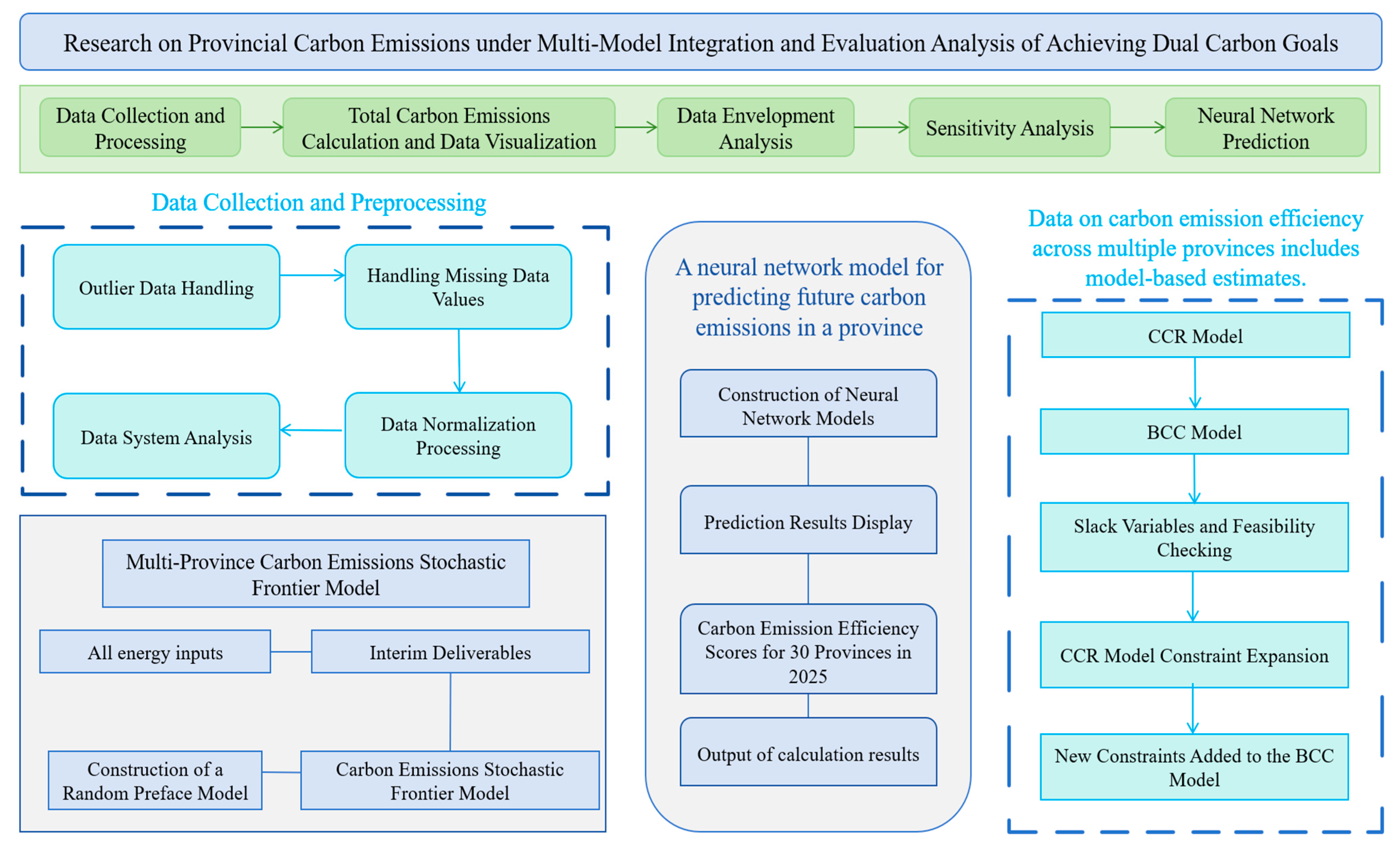
The specific research content of this study is shown in Figure 1: Research content roadmap.

3.1. Data Sources

This study focuses on the analysis of provincial carbon emissions. Data on the consumption of various types of energy in 30 provinces in China (excluding Taiwan, Hong Kong, Macao, and Tibet) were collected from the China Statistical Yearbook [35] and the Blue Map [36]. These data were converted into carbon content using heating values and carbon content per unit calorific value to ensure uniformity.
Economic data: Population size and GDP data of each province over the years were obtained from the China Statistical Yearbook. Population size reflects the labor force scale and consumer market size of a region, while GDP is a core indicator for measuring the economic development level of a region. Both are of great significance for studying the relationship between carbon emissions and economic development.
Energy consumption data: Data on the consumption of various energy sources such as coal, oil, and natural gas in each province were also collected from the China Statistical Yearbook and the Blue Map. As traditional fossil energy sources, coal and oil account for a large proportion of the energy consumption structure, and their consumption directly affects the total carbon emissions. These energy consumption data are the basis for calculating carbon emissions and provide key information for studying the relationship between energy consumption and carbon emissions.
Carbon emission parameter data: To accurately calculate carbon emissions, data on the heating values and carbon content per unit calorific value of different energy types were collected, as shown in Table 1: Conversion standards for various fuel data. These parameters are used to convert energy consumption into carbon content, ensuring the accuracy and scientificity of carbon emission calculation.
Based on the statistical data of the past decade (2010–2020), a significant positive correlation can be observed between the increase in coal mining and the growth of investments in roads, construction, and industry in several Chinese provinces. This correlation is not coincidental but reflects a deep-seated economic development pattern: regions with high coal output, such as Shanxi, Shaanxi, and Inner Mongolia, often simultaneously serve as key areas for energy-intensive industries. The expansion of coal mining directly drives local demand for heavy-haul roads (for coal transportation) and industrial fixed-asset investments (for washing, processing, and chemical conversion). Simultaneously, the fiscal revenue generated from the coal industry provides the financial foundation for these regions to fund large-scale infrastructure construction, including urban roads and real estate development. Therefore, the relationship among the three has formed a mutually reinforcing cycle: coal fuels industry and infrastructure, which in turn create sustained demand for coal. This synergy is a crucial explanation for why some provinces maintain high carbon emission lock-in effects while facing challenges of “scale inefficiency” in the subsequent efficiency analysis.

3.2. Data Preprocessing

3.2.1. Outlier Handling

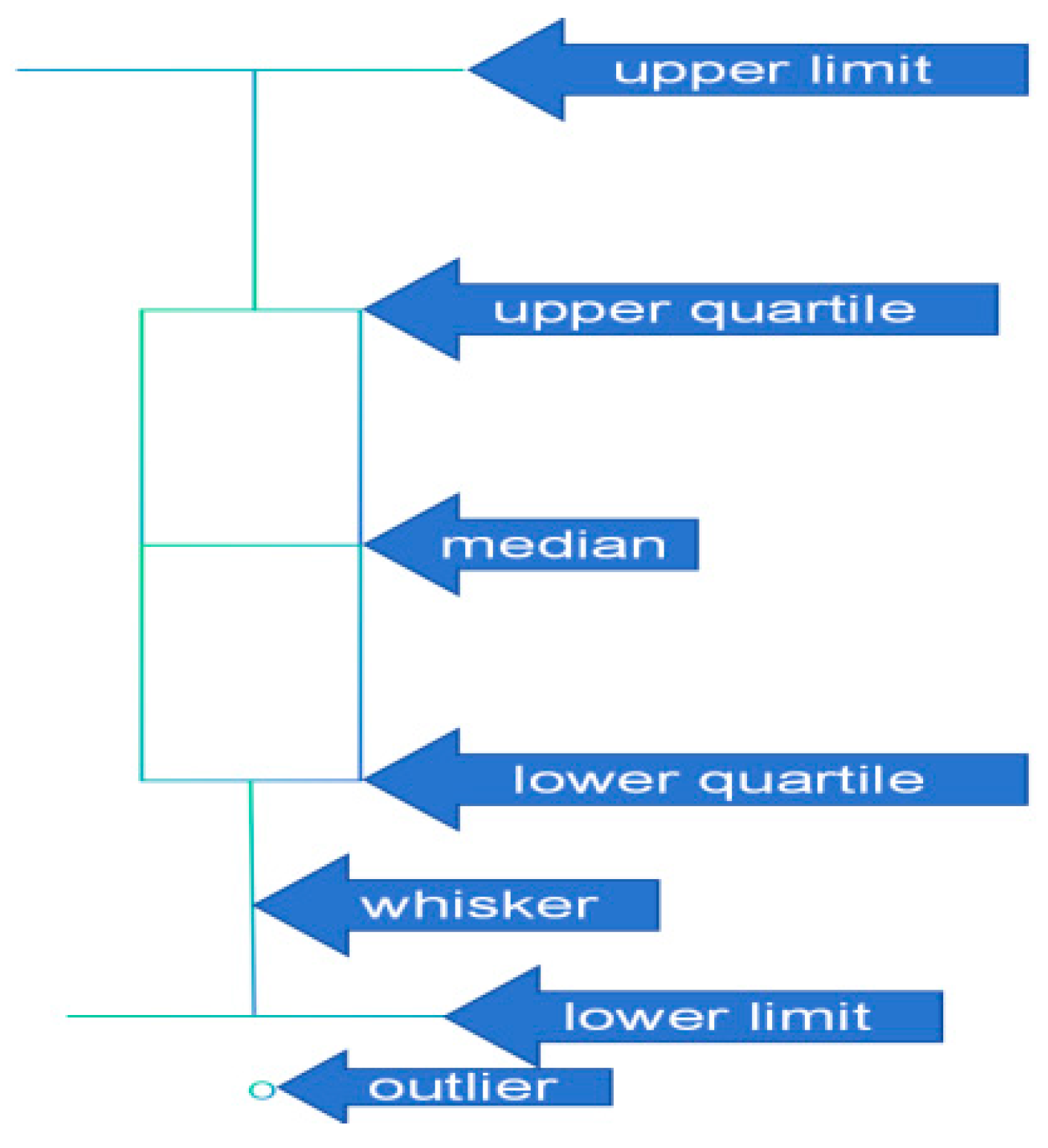
For outliers, the IQR (interquartile range) outlier identification method was adopted. The interquartile range is the difference between the upper quartile (Q3) and the lower quartile (Q1). Using 1.5 times the IQR as the standard, a data point xi is defined as an outlier if it satisfies xi < Q1 − 1.5 × IQR or xi > Q3 + 1.5 × IQR. Q1 is the value at the 25th percentile of all sample values sorted in ascending order, and Q3 is the value at the 75th percentile. This is illustrated in Figure 2: Schematic diagram of IQR outlier identification.
I Q R = Q 3 Q 1

3.2.2. Missing Value Handling

First, Lagrange interpolation was used to fill in the missing data of 2005–2019 in each worksheet. Lagrange interpolation is a polynomial interpolation method: for n + 1 distinct points x0, x1, …, xn and their corresponding function values y0, y1, …, yn, there exists a unique polynomial p n ( x ) with a degree not exceeding n such that p n x i = y i i = 1 , 2 , , n + 1 . The Lagrange interpolation basis function is:
l i ( x ) = j = 0 j i n x x j x i x j
The interpolation polynomial is:
p n ( x i ) = y i ( i = 1 , 2 , , n + 1 )
l 0 x = x x 1 x 0 x 1 , l 1 ( x ) = x x 0 x 1 x 0
When n = 1, it degenerates to linear interpolation: p 1 ( x ) = y 0 l 0 ( x ) + y 1 l 1 ( x ) .
This method can directly obtain the interpolation polynomial by constructing basis functions without solving linear equations and is suitable for approximating complex curves with simple curves (such as quadratic curves).
Considering that different input and output indicators may have different dimensions and units, normalization was performed. In the evaluation of carbon emission efficiency, the output indicators include population size (10,000 people) and GDP (100 million yuan); the input indicators include the consumption of various energy sources (10,000 tons) and the corresponding energy carbon content (tC). These different dimensions lead to large differences in the numerical values of each indicator. Without normalization, indicators with large numerical values may dominate the model, overshadowing the impact of other indicators. Through normalization, all indicators are converted to numerical values of the same order of magnitude, ensuring that each indicator has equal importance in the model and can participate in the calculation of efficiency values more fairly.
The Min–Max normalization method was used
X n o r m = X X m i n X m a x X m i n
where X is the original data, X m i n is the minimum value of the indicator in the dataset, X m a x is the maximum value of the indicator in the dataset, and X n o r m is the normalized data, which ranges from [0, 1]. This method maps the original data to the [0, 1] interval through linear transformation. It scales the data based on the value range, retains the original distribution shape of the data, and only compresses it into a fixed interval. It is suitable for situations where the data distribution is relatively stable and it is desired to limit the data to a specific interval.

4. Descriptive Statistical Analysis

For the processed data, descriptive statistical methods were used in this study to identify correlations and differences between the data. Some relevant data are shown in Table 2.

4.1. Carbon Emission Analysis by Region

4.1.1. North China and East China

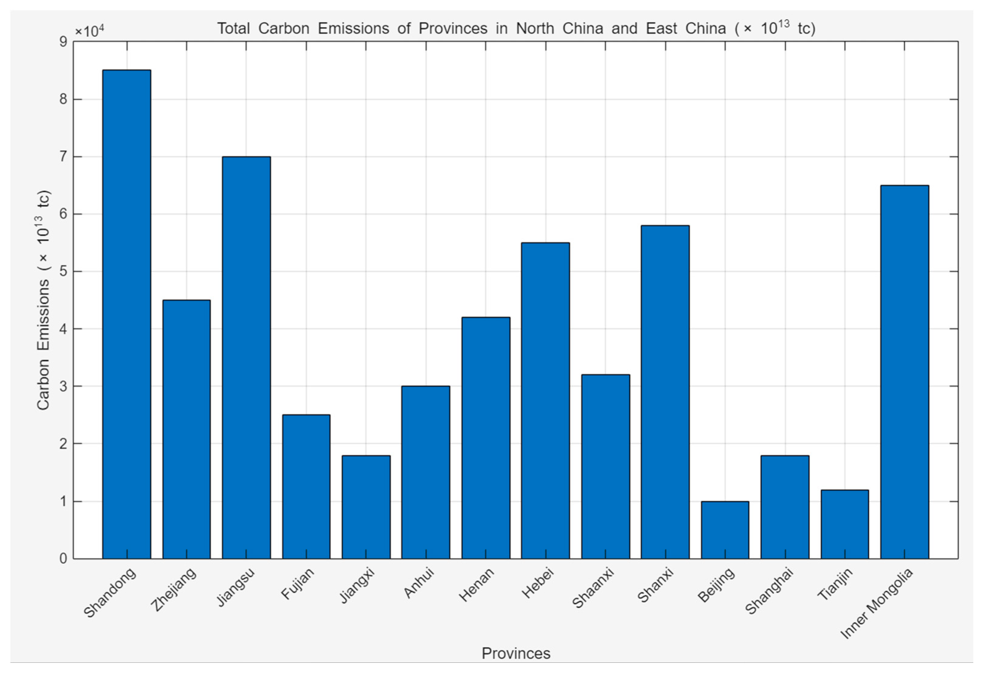
As shown in Figure 3: Total carbon emissions of provinces in North China and East China (×1013 tC), Shandong Province has the highest total carbon emissions, approaching 8 × 10¹⁴ tC, which is significantly higher than other provinces and becomes the “peak” of carbon emissions in this region. Provinces/municipalities such as Tianjin and Beijing have relatively low emissions, among which Tianjin may have the lowest emissions in the figure, reflecting the small scale of carbon emissions in these regions within the area. The carbon emissions of various provinces differ significantly: Shandong has the highest emissions, while some provinces (such as Tianjin and Beijing) have emissions much lower than the average, indicating an extremely unbalanced level of carbon emissions in the region, with a large standard deviation and high dispersion.

4.1.2. Northeast China

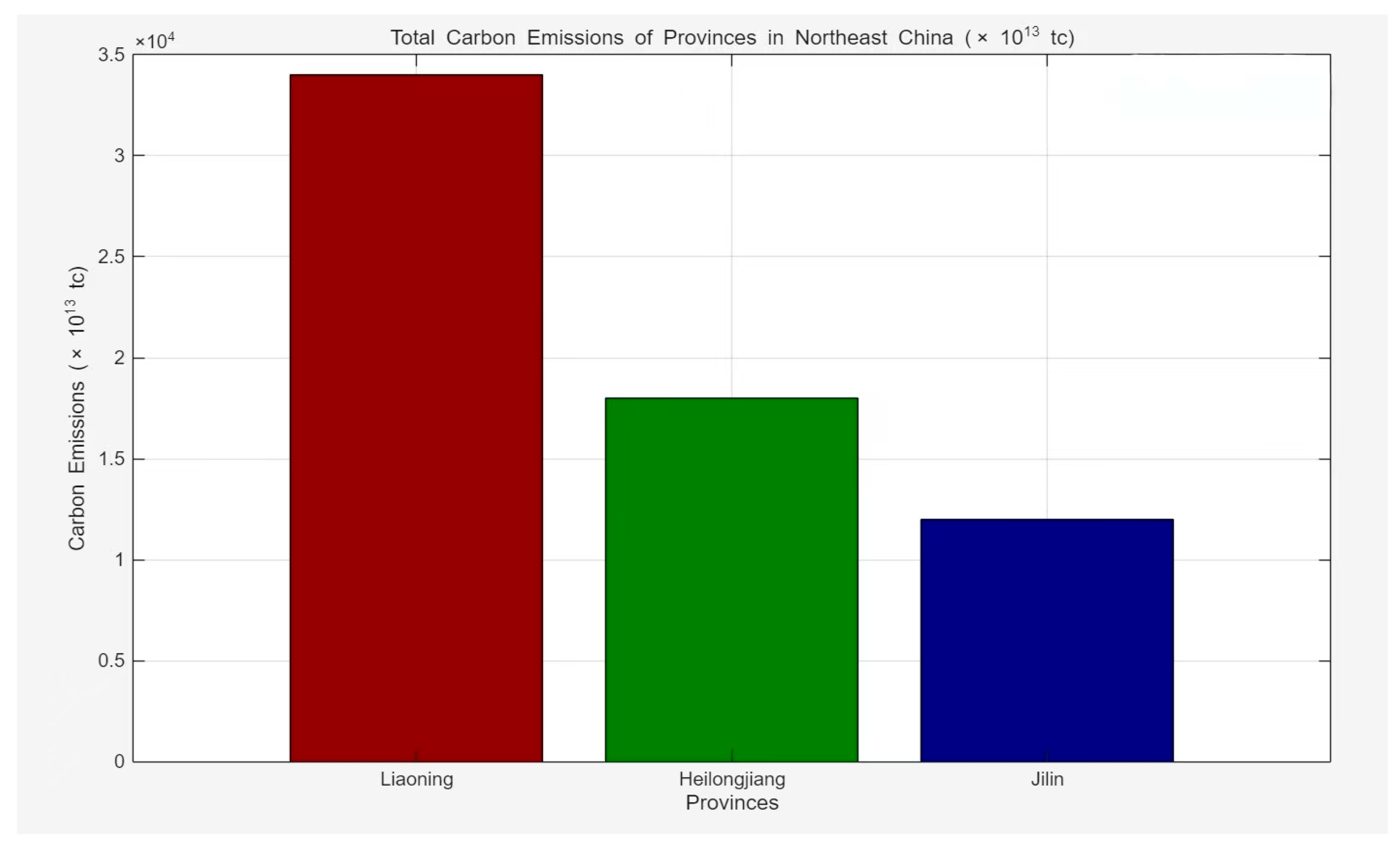
As shown in Figure 4, Liaoning Province has the highest total carbon emissions, leading in Northeast China. Jilin Province has the lowest total carbon emissions, approximately 1 × 10¹⁴ tC, which is significantly lower than Liaoning. The total carbon emissions of the three provinces differ significantly, and the gap between Liaoning and Heilongjiang/Jilin is large, indicating an unbalanced level of carbon emissions within Northeast China, with a relatively high standard deviation and high dispersion.

4.1.3. Northwest and Southwest China

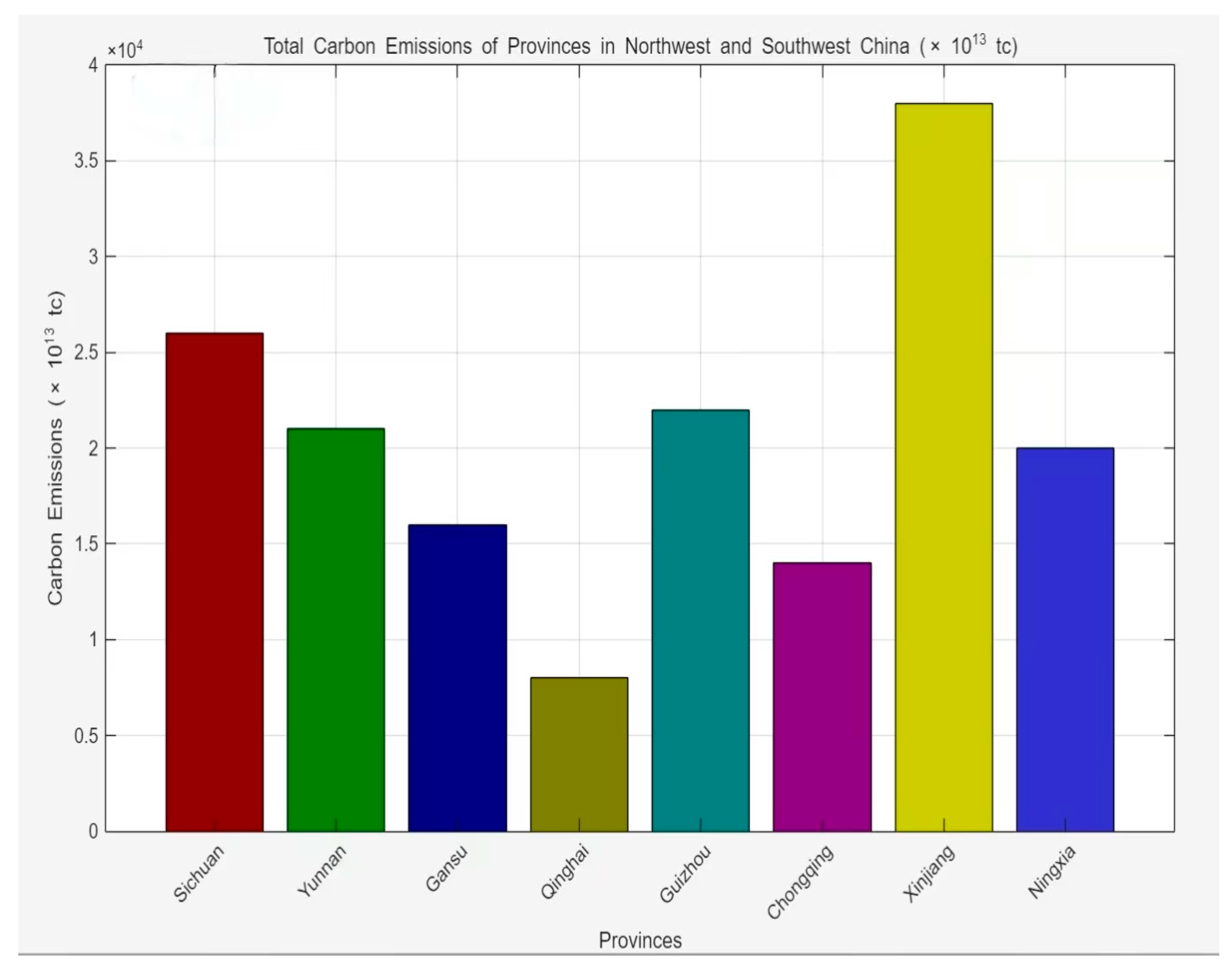
As shown in Figure 5, Xinjiang Uygur Autonomous Region has the highest total carbon emissions, approaching 4 × 10¹⁴ tC, leading in this region. Qinghai Province has the lowest total carbon emissions, significantly lower than other provinces, at approximately 5 × 10¹³ tC. Provinces such as Sichuan, Guizhou, and Ningxia Hui Autonomous Region have emissions in the middle range: for example, Sichuan is approximately 2.5 × 10¹⁴ tC and Guizhou is approximately 2 × 10¹⁴ tC, but there are still obvious gaps between provinces. The total carbon emissions of various provinces differ significantly, and the gap between Xinjiang Uygur Autonomous Region and Qinghai/Gansu is large, indicating an unbalanced level of carbon emissions within Northwest and Southwest China, with a high standard deviation and high dispersion.

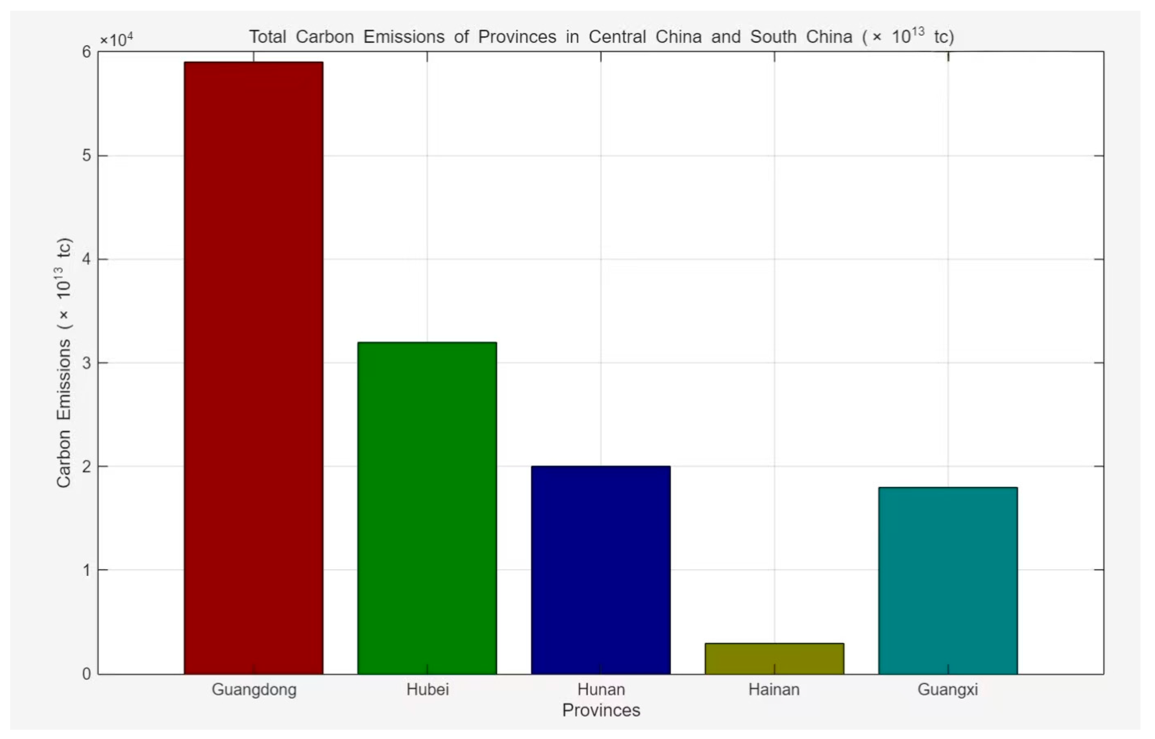
4.1.4. Central China and South China

As shown in Figure 6, Guangdong Province has the highest total carbon emissions, approaching 6 × 10¹⁴ tC, with the largest scale of carbon emissions in Central and South China. Hainan Province has the lowest total carbon emissions, significantly lower than other provinces, reflecting its extremely small scale of carbon emissions. Hubei, Hunan, and Guangxi Zhuang Autonomous Region are in the middle range: Hubei is approximately 3 × 10¹⁴ tC, Hunan is approximately 2 × 10¹⁴ tC, and Guangxi Zhuang Autonomous Region is approximately 2 × 10¹⁴ tC, but there are still obvious gaps between provinces. The total carbon emissions of various provinces differ significantly, and the gap between Guangdong and Hainan is extremely large, indicating an extremely unbalanced level of carbon emissions within Central and South China, with a high standard deviation and high dispersion.

4.2. Residual Analysis of Provincial Indicators

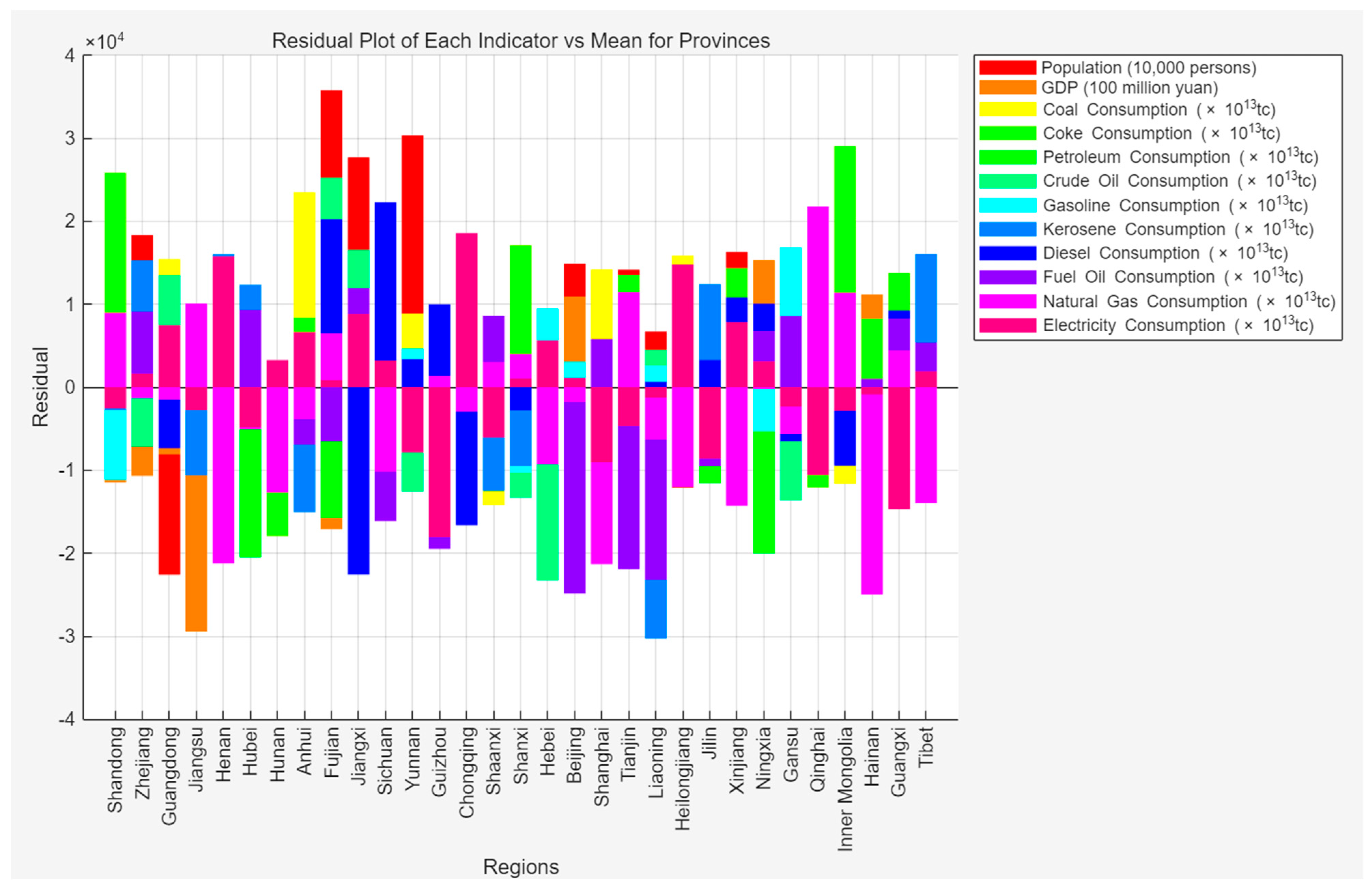
As shown in Figure 7, some provinces have large absolute residual values in specific indicators. For example, Shandong Province has much higher residuals than average in indicators such as oil and gasoline consumption carbon content (green and red), indicating that its consumption of these energy sources is far higher than the national average; while regions such as Tibet have residuals close to zero in most indicators, suggesting that their indicators are closer to the average. The residuals of energy consumption carbon content indicators fluctuate greatly, reflecting differences in energy consumption structure and scale among provinces. For example, economically developed provinces (such as Guangdong) have high residuals in some energy indicators, which is related to their industrial scale and energy demand; some western provinces (such as Xinjiang) have prominent residuals in certain energy indicators, which may be related to resource development and industrial characteristics.
This figure intuitively presents the deviation of each province from the national average in multiple indicators, providing a visual basis for analyzing regional economic and energy consumption characteristics and differences, and facilitating targeted research on the development models and energy consumption structures of provinces with high deviations.
In summary, there are significant differences in carbon emissions between different regions, and the differences between provinces are even more obvious. There are individual provinces with high emissions (such as Shandong) and many provinces with medium and low emissions. This distribution may be related to factors such as the industrial structure of each province (e.g., Shandong has a developed industry and high energy consumption), economic scale, and energy structure. Therefore, the evaluation and analysis of this study are imperative. In the subsequent research, combined with specific data envelopment and stochastic frontier models, the causes of carbon emission differences will be further explored to provide a basis for formulating regional carbon emission reduction policies (e.g., strengthening energy consumption control in high-emission provinces and promoting green development experience in low-emission provinces).

4.3. Discussion on the Parallel Development of Renewable Energy in High-Emission Regions

Based on the carbon emission distribution characteristics revealed in the previous sections, it is essential to further explore whether high-emission regions are simultaneously advancing the deployment of renewable energy installations. In provinces such as Shandong, Guangdong, Hebei, and Inner Mongolia—where total carbon emissions are notably high and energy consumption structures remain heavily reliant on fossil fuels—observing the parallel developmwent of renewable energy infrastructure becomes critical for evaluating regional decarbonization pathways. In recent years, several of these high-emission regions have indeed accelerated the construction of wind, solar, and other renewable energy facilities as part of national energy transition strategies. For example, Shandong has promoted large-scale offshore wind power projects, Inner Mongolia leads in onshore wind and photovoltaic bases, and Guangdong has expanded its renewable energy capacity alongside industrial growth. However, the pace and scale of such deployments vary significantly across regions, influenced by local resource endowments, policy support, and economic conditions. Therefore, while high-emission regions are increasingly investing in clean energy, the extent to which these installations offset carbon emissions remains uneven. This observation underscores the need for integrating renewable energy development into efficiency evaluations and future scenario simulations, ensuring that emission reduction strategies are both technically feasible and regionally adaptable. The subsequent chapters will further quantify these dynamics through efficiency decomposition and predictive modeling.

5. Research on Data Envelopment Model for Carbon Emission Efficiency of Multiple Provinces

5.1. Construction of Data Envelopment Model

Data envelopment analysis (DEA) is a non-parametric statistical method used to evaluate the relative efficiency of decision-making units (DMUs). It constructs a production frontier, projects the input and output data of each DMU onto this frontier, and judges the relative efficiency of DMUs by comparing their distance from the frontier. In the model, each province was selected as a different DMU (e.g., Shandong, Liaoning), energy carbon content (e.g., natural gas, oil) was selected as an input indicator, and population and GDP were selected as output indicators. DMUs on the frontier are considered efficient, while those deviating from the frontier are considered inefficient, and the degree of inefficiency can be measured by the distance from the frontier.
Assuming that the evaluation objects are 30 provinces as DMUs, each DMU includes an 11-dimensional input vector and a 2-dimensional output vector:
X j = X 1 j , X 2 j , , X 11 j , Y j = ( y 1 j , y 2 j ) T ( j = 1 , 2 , , n ) . The production possibility set is defined as the set of all feasible production combinations, where λ j is the combination weight of DMUs, reflecting the construction logic of the production frontier.
In the evaluation of provincial carbon emission efficiency, this study selects the CCR model under constant returns to scale and the BCC model under variable returns to scale. The setting of returns-to-scale assumptions is not an arbitrary methodological choice, but a theoretical modeling of the scalability characteristics of provincial economic systems. Its selection must be consistent with the production technology structure of decision-making units and the realistic evolution logic of carbon emissions.
The assumption of constant returns to scale in the CCR model is primarily suited to the realistic characteristics of developed coastal provinces in eastern China, where carbon emission-related production activities have approached the optimal production scale, energy utilization technologies are mature, and factor allocation efficiency is high. Meanwhile, this assumption can eliminate the interference of initial provincial scale differences on efficiency measurement, provide a unified, scale-unbiased efficiency reference system for 30 provinces nationwide, and meet the demand for comparable quantification of inter-regional carbon emission efficiency. It also serves as an important logical premise for decomposing comprehensive technical efficiency into pure technical efficiency and scale efficiency. In contrast, the BCC model relaxes the assumption from constant to variable returns to scale, which precisely fits the core feature of remarkable disparities in resource endowments, industrial structures and development stages among China’s provinces. It is especially applicable to provinces in central and western regions where some clean energy industries are in the cultivation stage, featuring increasing returns to scale and great potential for scale expansion.
Furthermore, the combined application of the CCR and BCC models achieves a dual adaptation between theoretical assumptions and the realistic scalability of provincial carbon emissions. It not only reflects the unified goal of national carbon emission reduction governance and provides an unbiased benchmark for cross-provincial carbon emission efficiency comparison, but also accommodates the heterogeneous reality of provincial development and realizes the refined decomposition of carbon emission efficiency. This allows the efficiency analysis results to directly match the carbon emission reduction practice needs of different provinces, providing a scientific economic basis for the formulation of differentiated emission reduction policies.

5.1.1. CCR Model (Constant Returns to Scale, CRS)

Proposed by Charnes, Cooper and Rhodes (1978), the CCR model assumes that production technology satisfies constant returns to scale (CRS), with the core goal of measuring the technical efficiency (TE) of DMUs [3].
(1)
Input-Oriented Model
The original fractional programming (for the 30th DMU) is
θ k = min θ , u , v θ u T y j s . t . v T x j u T y j 1 , j = 1,2 , , n ; v 0 , u 0
where v is the input weight vector, u is the output weight vector, and θ is the efficiency value (compression ratio).
Through the Charnes–Cooper transformation (converted to linear programming):
θ k = min θ
s . t . j = 1 n λ j x i j θ x i k , i = 1 , 2 , , 11
j = 1 n λ j y r j y r k , r = 1 , 2 , , s
λ j 0 , j = 1,2 , , n
Objective function: Minimize the input compression ratio θ (a DMU is inefficient if θ ≤ 1, and technically efficient if θ = 1).
Constraints: Construct the frontier, requiring that the input of the reference combination does not exceed θ times the input of the target DMU, and the output is not lower than the output of the target DMU.
(2)
Economic Implications
Technical efficiency: If θ = 1 and all slack variables are zero, the DMU is on the production frontier (Pareto efficient).
Input redundancy: If j = 1 n λ j x i j < θ x i k , there is redundancy in the i-th input, and the redundancy amount is:
x i k j = 1 n λ j x i j

5.1.2. BCC Model (Variable Returns to Scale, VRS)

Proposed by Banker, Charnes and Cooper (1984), the BCC model introduces a convexity assumption and assumes that production technology satisfies variable returns to scale (VRS), decomposing technical efficiency into pure technical efficiency (PTE) and scale efficiency (SE) [37].
A convex combination constraint is added to the CCR model:
j = 1 n λ j = 1
ψ k = min ψ s . t . j = 1 n λ j x i j ψ x i k , i = 1,2 , , 11 j = 1 n λ j y r j y r k , i = 1,2 j = 1 n λ j = 1 λ j 0 , j = 1,2 , , n
Pure technical efficiency (PTE): Reflects the technical efficiency of DMUs after excluding scale factors (only evaluating the resource utilization efficiency at the management or technical level).

5.1.3. Scale Efficiency (SE)

Scale efficiency is calculated through the relationship between CCR and BCC efficiency values:
S E = θ k ψ k
Returns-to-scale status:
If j = 1 n λ j < 1 , increasing returns to scale (IRS);
If j = 1 n λ j > 1 , decreasing returns to scale (DRS);
If j = 1 n λ j = 1 , constant returns to scale (CRS, corresponding to CCR efficient points).

5.2. Results Analysis

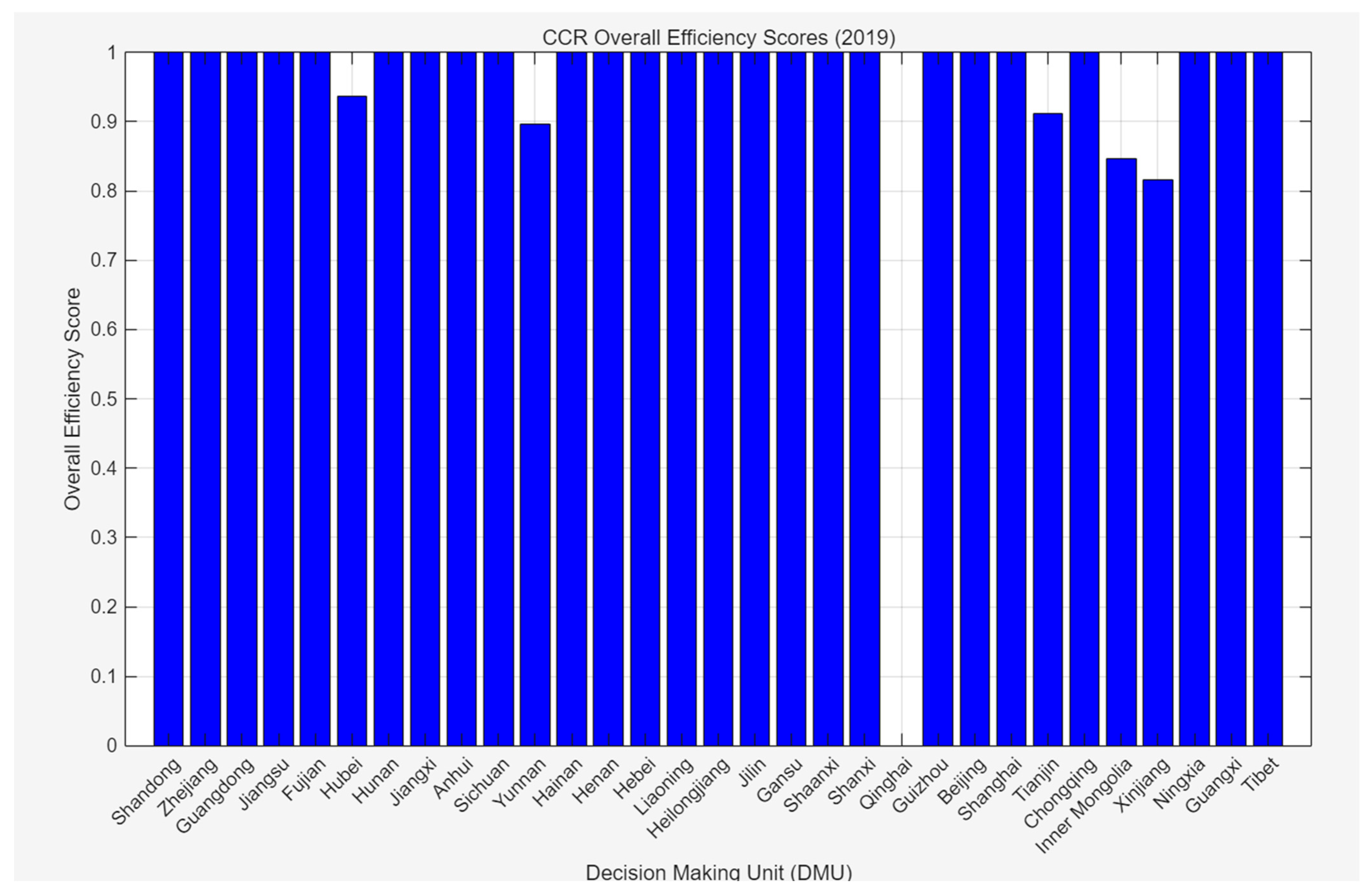
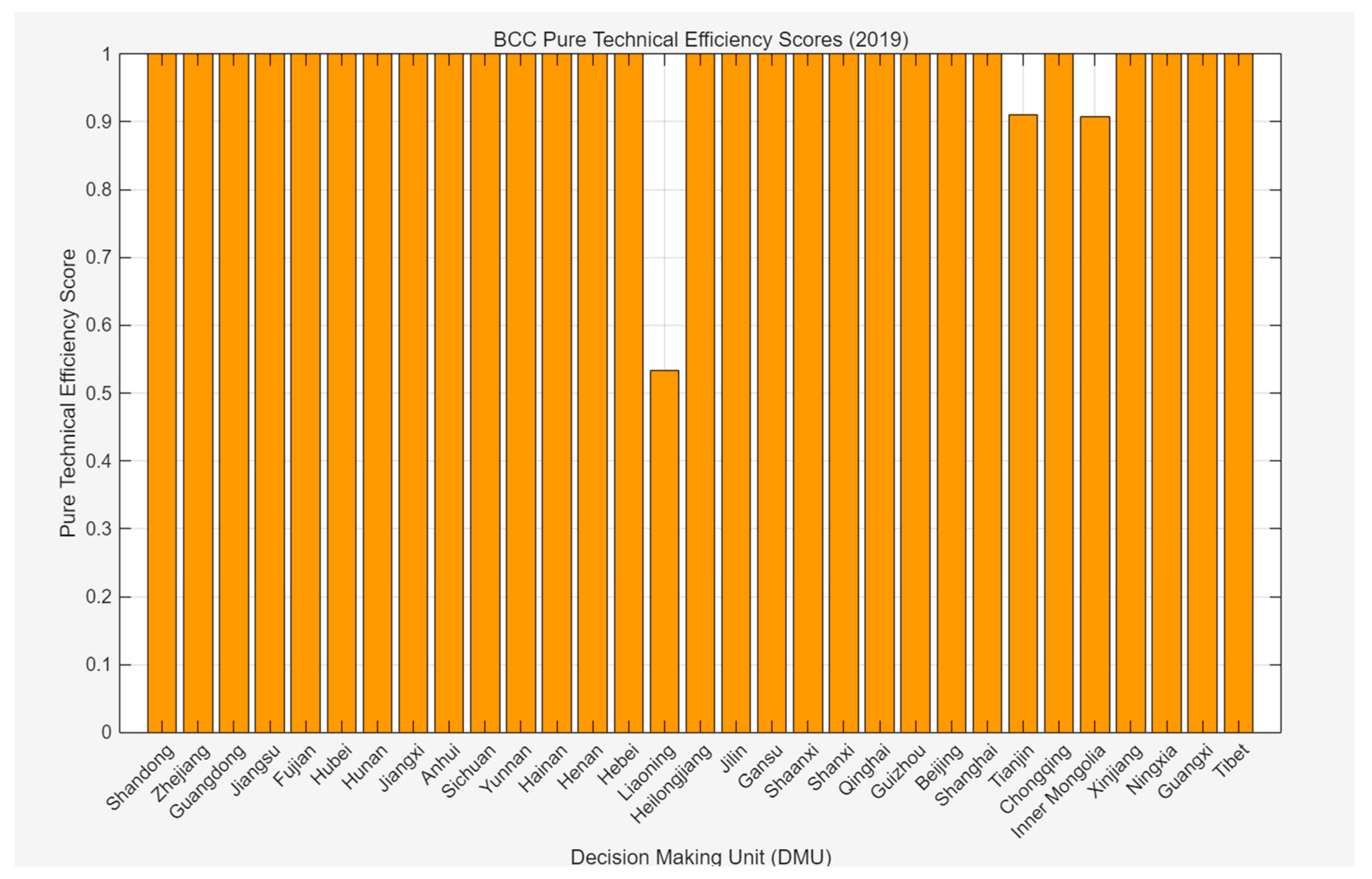
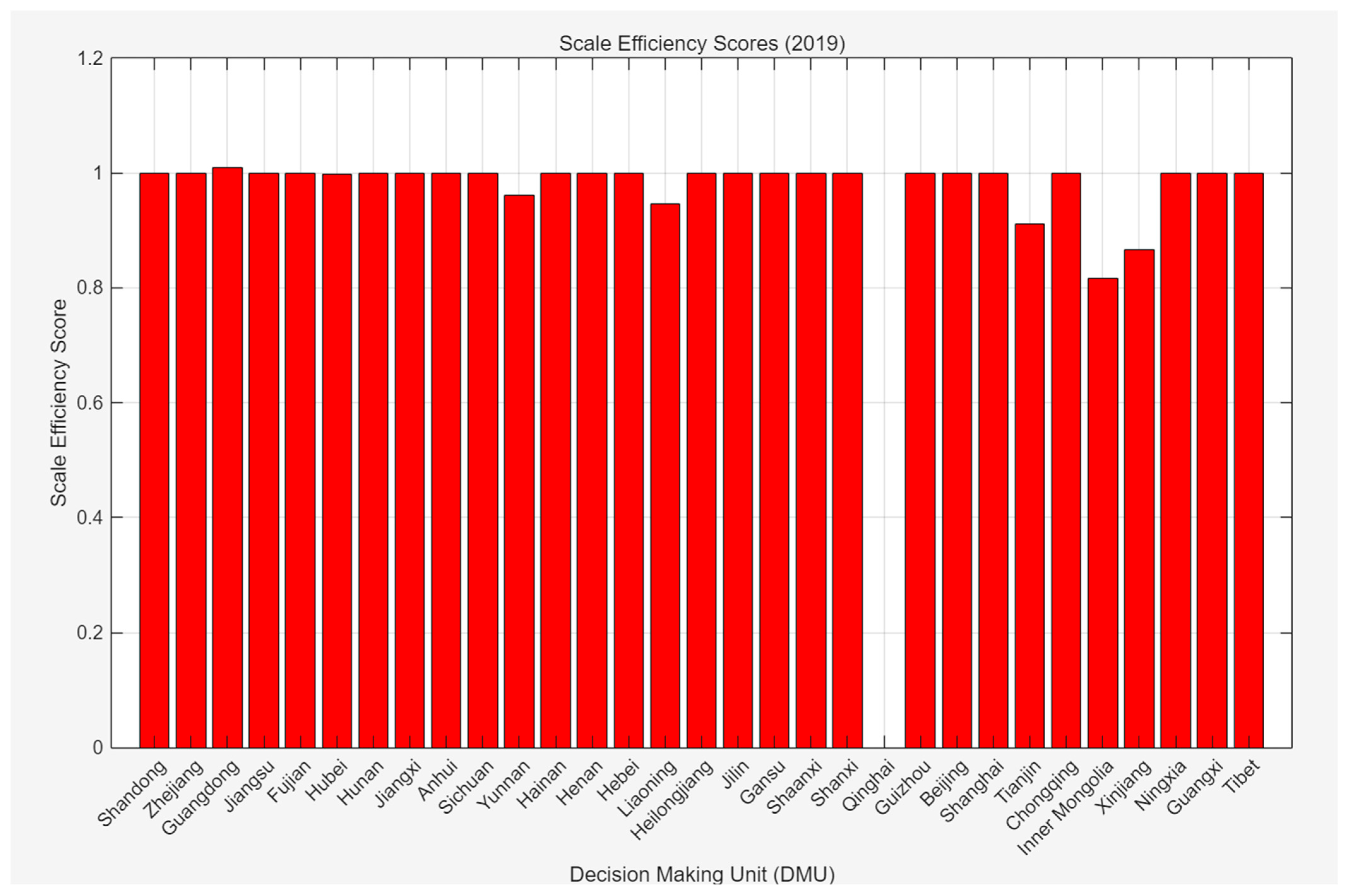
As shown in Figure 8: Bar chart of BCC efficiency scores (2019); Figure 9: Bar chart of CCR efficiency scores (2019); Figure 10: Bar chart of scale efficiency scores (2019); Table A1: 2019 model efficiency scores of provinces in Southwest and Northwest China; Table A2: 2019 model efficiency scores of provinces in Central China, South China, and Northeast China; and Table A3: 2019 model efficiency scores of provinces in North China and East China, from the perspective of regional energy efficiency, eastern coastal provinces and most municipalities directly under the Central Government perform well. Economically developed regions such as Shandong, Zhejiang, Guangdong, Jiangsu, and Fujian have advanced technologies and high energy utilization efficiency. For example, Guangdong has reached the frontier level in the technical transformation efficiency of the oil industry chain, and Jiangsu has high GDP output and strong energy management capabilities. Municipalities directly under the Central Government dominated by the service industry, such as Beijing and Shanghai, have low demand for high-carbon energy and significant advantages in technical efficiency.
Among regions with low technical efficiency, Hubei, Hunan, Hebei, and Inner Mongolia have problems to varying degrees: Hubei has a relatively high proportion of heavy industry due to high carbon content in coal and coke consumption, and its energy conversion technology or management needs improvement; Hunan’s energy structure is dominated by coal, and its carbon content in coke and oil consumption is higher than that of efficient regions, so its technical efficiency is dragged down by traditional industries; Hebei has high carbon content in coal and coke consumption (with large steel production in the province), and its technical efficiency is significantly lower than other regions, requiring the promotion of low-carbon technology upgrading in the steel industry; as a major coal-producing area, Inner Mongolia has the second-highest carbon content in coal consumption after Shanxi, and its energy extraction and conversion technology efficiency is close to the frontier but still has room for improvement.
In terms of CCR comprehensive efficiency, 22 regions (accounting for 73%), including Guangdong, Jiangsu, Zhejiang, and Shandong, have efficient matching between energy input and population/GDP output, with both technical effectiveness and scale rationality. Among regions with low comprehensive efficiency, Hubei’s comprehensive efficiency is slightly lower due to a slight decline in technical efficiency, requiring the optimization of energy technology; Hunan has a dual decline in technical efficiency and scale efficiency, reflecting technical bottlenecks and excessive scale under high-carbon input; Hebei’s extremely low technical efficiency is the main reason, requiring priority to improve energy utilization technology; Chongqing has high carbon content in natural gas and electricity consumption and low scale efficiency, requiring technical optimization and control of energy input scale; and Inner Mongolia and Xinjiang have decreasing returns to scale due to high coal consumption and low efficiency in oil and natural gas extraction and conversion, respectively.
In terms of scale efficiency, 23 regions (accounting for 77%) have matching energy input scale and output, and Guangdong and Jiangsu have achieved economies of scale through industrial agglomeration. Among regions with low scale efficiency, Hubei’s scale efficiency has slightly declined, and the focus should be on improving technical efficiency; Hunan and Hebei have excessive high-carbon energy input, requiring a reduction in inefficient production capacity; Qinghai has abnormal data due to extremely small input–output scale, requiring correction based on actual conditions; and Chongqing, Inner Mongolia, and Xinjiang have the problem of “scale expansion faster than efficiency improvement”—Inner Mongolia relies on coal mining and Xinjiang relies on petrochemical industry, both of which need to control the scale of high-carbon industries and shift to clean energy deep processing.
Overall, eastern coastal provinces and municipalities directly under the Central Government have become efficiency benchmarks relying on technological advantages and industrial structure optimization, while regions with concentrated high-carbon heavy industries such as Hebei, Inner Mongolia, and Hunan have low efficiency due to technical bottlenecks and unreasonable scales. In the future, regions with low technical efficiency should prioritize upgrading low-carbon technologies in high-carbon industries; regions with low scale efficiency need to control excess production capacity and shift to the extension of clean energy industrial chains; and Qinghai, with abnormal data, needs to incorporate new energy industry data for correction and analysis. Targeted policies will promote the balanced improvement of national energy efficiency.

5.3. Implicit Consideration of Combustion Technology Efficiency in the Model

It is important to clarify whether the carbon emission efficiency model explicitly incorporates factors related to the development of new, more efficient installations for burning coal and hydrocarbons. In the current data envelopment analysis (DEA) framework, the model does not include a separate, independent variable labeled “combustion technology level” or “installation efficiency.” Instead, the impact of such technological advancements is implicitly captured through the efficiency evaluation mechanism itself. Specifically, when a province invests in higher-efficiency coal-fired power plants or upgrades industrial boilers to reduce carbon intensity per unit of energy consumed, these improvements are reflected in the input–output relationship: the same amount of energy input (measured in tons of coal or oil) yields higher outputs (GDP and population services), or alternatively, lower carbon content is associated with the same output level. In DEA, provinces that adopt such advanced combustion technologies will appear closer to or on the production frontier, resulting in higher technical efficiency scores. Therefore, while the model does not directly measure “installation efficiency” as a distinct input, the consequences of such technological progress—reduced waste and higher output per unit of carbon—are embedded in the efficiency scores.

6. Neural Network Model for Predicting Future Carbon Emissions of Various Provinces

6.1. Construction of Neural Network Model

Long short-term memory (LSTM) is a special Recurrent Neural Network (RNN) proposed by Hochreiter and Schmidhuber (1997) to solve the long-distance dependence problem in traditional RNNs (e.g., difficulty in learning long-term dependencies due to gradient disappearance) [38]. By introducing a gating mechanism, LSTM can selectively remember or forget information, effectively processing long-time-series data, and is widely used in fields such as Natural Language Processing (NLP), time-series prediction, and speech recognition.
An LSTM unit consists of four core components: a forget gate that determines which information to forget from the cell state; an input gate that determines which new information to input into the cell state; a candidate cell state that generates candidate states to be updated; and an output gate that determines the final output hidden state.

6.2. Formula Derivation

Assuming that the input at time t is Xt, the hidden state at the previous time t − 1 is ht−1, the cell state is Ct−1, each parameter matrix is W, and the bias is b.
Forget gate: Determines which information to discard from the cell state:
f t = σ ( W f [ h t 1 , x t ] + b f )
Input gate: Determines the new information to be added to the cell state, including two parts:
Candidate cell state (new information generated by tanh):
C ~ t = tanh ( W C [ h t 1 , x t ] + b C )
Input gate weight (determines how much candidate information to accept):
i t = σ ( W i [ h t 1 , x t ] + b i )
Update cell state: Combine the forget gate and input gate to update the cell state:
C t = f t C t 1 + i t C ~ t
Output gate: Determine the final output hidden state:
h t : ( o t = σ ( W o [ h t 1 , x t ] + b o )
h t = o t tanh ( C t )

6.3. Solution of LSTM Model

In this study, the parameter settings and selection logic of the model are as follows. In terms of network structure, the model includes 1 LSTM hidden layer and 1 fully connected output layer, totaling 2 layers; the LSTM hidden layer is set with 50 neurons to capture the long-term dependence of time-series data related to provincial carbon emissions (such as energy consumption and GDP), and the number of neurons in the output layer is consistent with the dimension of the prediction target, matching 13 indicators including population, GDP, and 11 types of energy consumption. The forget gate parameters of LSTM units are not manually preset with a fixed forget rate, but are automatically learned through model training, and the information retention and discard ratio are dynamically optimized according to the characteristics of carbon emission time series. In terms of step size (sequence length), combined with the 11-year time-series data span from 2009 to 2019 in the study, a 3-year time window length was selected to predict the trend of subsequent years through the economic, energy, and carbon emission data of previous years, ensuring that the temporal correlation of the data can be effectively captured. Finally, the carbon emission prediction accuracy in 2019 is controlled within 8.7%, and the 2025 carbon emission trend is accurately simulated.
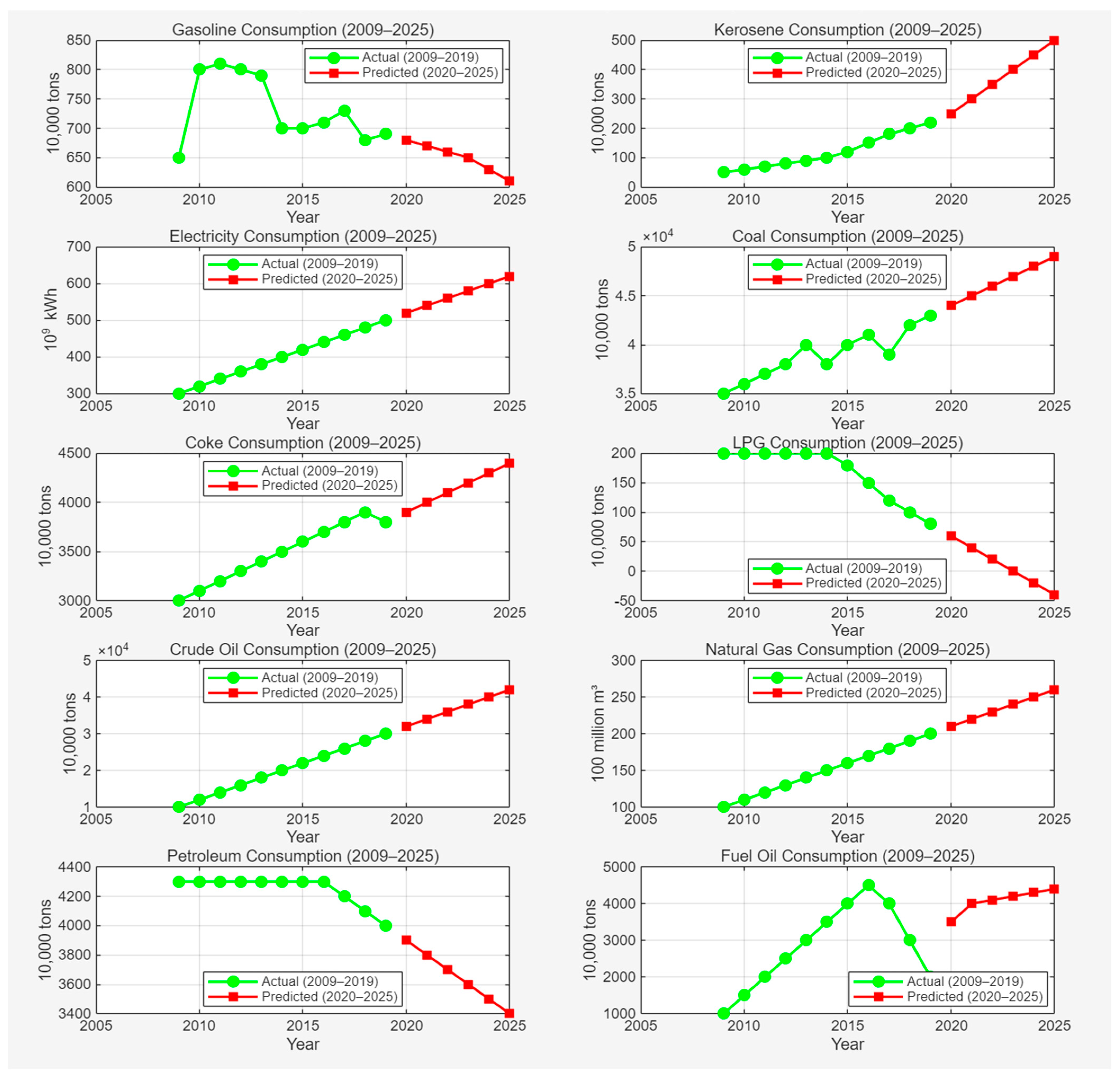
This section presents the solution of the LSTM model, and the following is a visual display of the prediction data of Shandong Province. Taking crude oil consumption prediction as an example, the actual values (2009–2019) show a steady upward trend, and the predicted values (2019–2025) continue this growth trend, with the upward trend connecting naturally with historical data, indicating that the model accurately captures the long-term growth trend of crude oil consumption; the actual values of electricity consumption (2009–2019) show steady growth, and the predicted values accelerate upward in the later period, which is in line with the logic of increasing electricity demand in economic development, and the trend remains consistent, indicating that the model is reasonable in predicting the long-term growth of electricity consumption.
As shown in Figure 11: Comparison between predicted and actual values of various resource consumption (Shandong Province, 2009–2025), in all LSTM prediction charts (such as crude oil, electricity, coal, and natural gas), the long-term trends of predicted values and actual values are basically consistent, and the model captures the growth logic of major energy consumption well. Overall, the model has certain rationality in trend prediction and can be used as a reference for energy planning.

6.4. Sensitivity Analysis

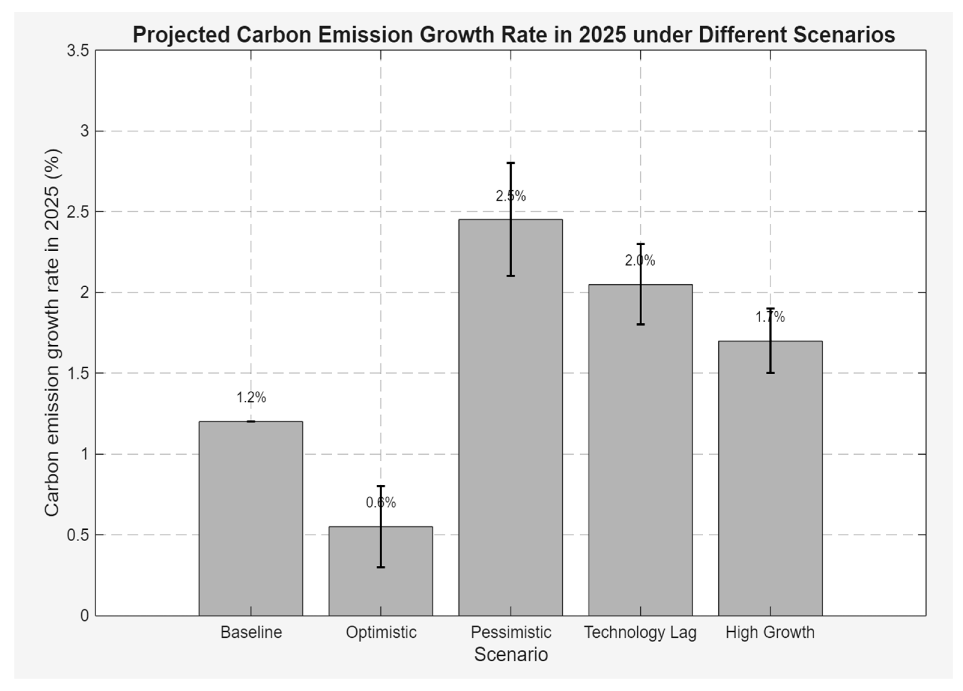
As shown in Figure 12, to verify the robustness of the carbon emission growth rate falling to 1.2% in 2025 when the clean energy proportion reaches 35%, we conducted a multi-scenario sensitivity analysis on key uncertain factors including policy implementation intensity, technology adoption rate, economic growth rate and power grid accommodation capacity. Five representative scenarios were constructed by adjusting the above parameters, and the carbon emission growth rate in 2025 under each scenario was recalculated based on the trained LSTM model.
The baseline scenario assumes that existing policies are fully implemented as planned, clean energy costs keep declining, the average annual economic growth rate stays at 5.0–5.5%, and grid accommodation capacity improves in tandem. Under this scenario, the clean energy share will reach 35%, corresponding to a growth rate of 1.2%. In the optimistic scenario, policy incentives outperform expectations, clean energy technologies achieve accelerated breakthroughs, and grid flexibility is substantially strengthened. The clean energy share rises to 38–40%, and the growth rate can fall to 0.6%, close to zero growth. The pessimistic scenario assumes delayed policy implementation, slow cost reduction in clean energy, and lagging grid upgrades. The clean energy share is only 28–32%, and the growth rate rebounds to 2.5%, more than double the baseline level. The technology lag scenario focuses separately on the constraint of grid accommodation capacity. Even if policy targets are achieved on schedule, a wind and solar curtailment rate above 10% leads to low actual utilization efficiency of clean energy, and the growth rate still reaches 2.0%. The high-growth scenario simulates the impact of above-expected economic growth (6.0–6.5% annually). With a clean energy share similar to the baseline, the increase in energy demand partially offsets the emission reduction effect, and the growth rate rises to 1.7%.
Sensitivity analysis indicates that policy implementation intensity is the most sensitive factor. The growth rate gap between the pessimistic and optimistic scenarios is nearly 2 percentage points, highlighting the key role of policy consistency. Grid accommodation capacity is the second most influential factor: the growth rate in the technology lag scenario is 0.8 percentage points higher than the baseline, demonstrating the importance of supporting infrastructure. The impact of economic growth is relatively mild but cannot be neglected.
Overall, the carbon emission growth rate in 2025 under all scenarios is significantly lower than the historical average of 5–6% from 2009 to 2019, verifying the robustness of the core conclusion: raising the clean energy share to around 35% can drive a trend decoupling between economic growth and carbon emissions. However, the specific emission reduction magnitude depends on the coordinated progress of policies, technologies and infrastructure.

6.5. Carbon Emission Efficiency Scores Analysis

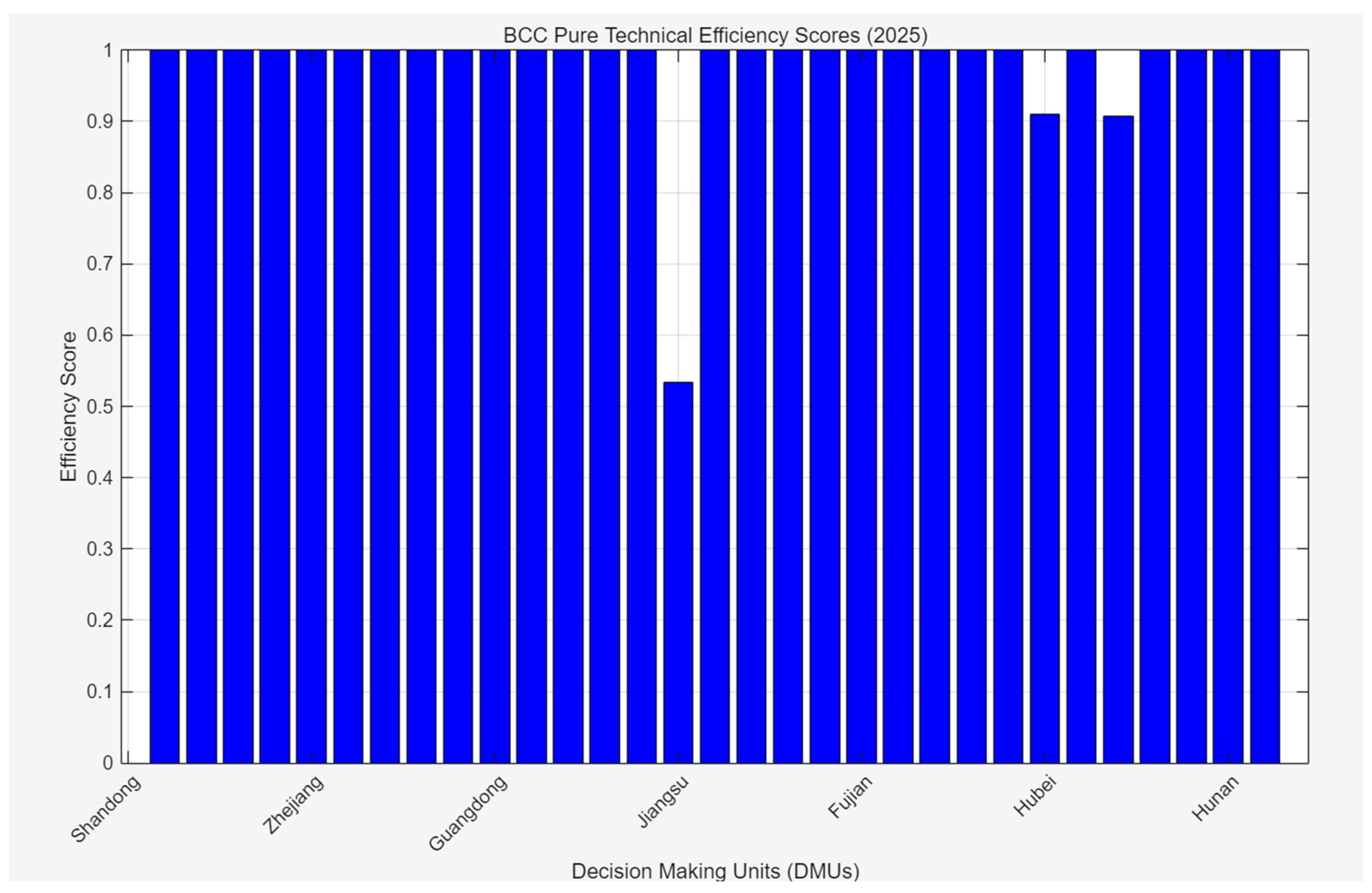
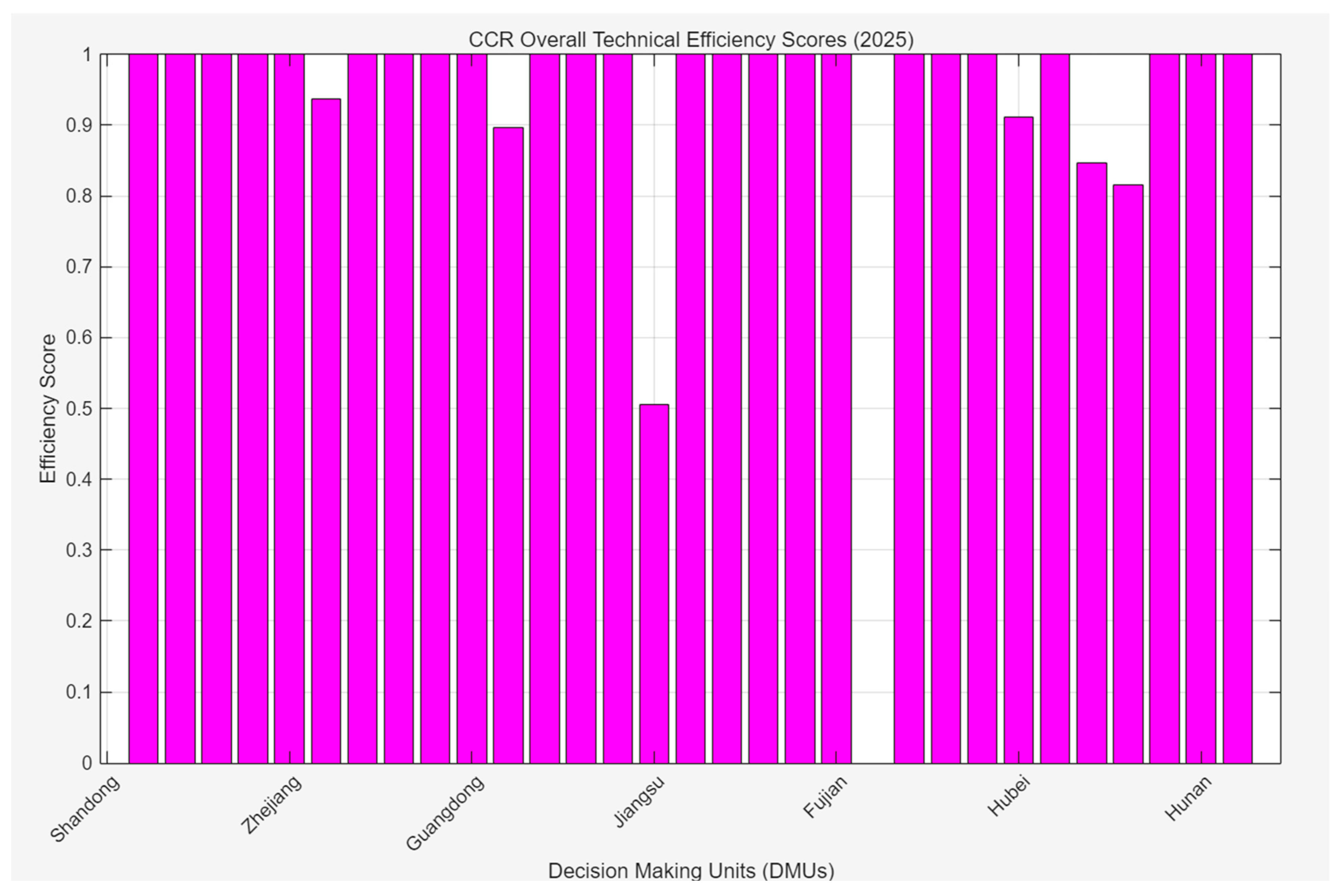
As shown in Figure 13, Figure 14 and Figure 15 and Table A4, Table A5 and Table A6: from the perspective of regional energy efficiency, economically developed eastern coastal provinces such as Shandong, Zhejiang, Guangdong, Jiangsu, and Fujian, as well as municipalities directly under the Central Government such as Beijing, Shanghai, and Tianjin, perform well in BCC pure technical efficiency. These regions have achieved efficient development with low carbon intensity per unit GDP and clean energy consumption structure, relying on mature energy utilization technologies, high-value-added industrial layouts (such as Guangdong’s electronic information industry and Zhejiang’s digital economy), and a clean industrial structure dominated by the service industry (Beijing’s tertiary industry accounts for 83%). For example, Guangdong has the highest penetration rate of new energy vehicles in the transportation sector in China, significantly reducing the carbon content of gasoline and diesel consumption.
Among provinces with low technical efficiency, Hubei has a high proportion of heavy industries such as steel and chemicals (Wuhan Iron and Steel’s production capacity accounts for 30% of the province), high carbon content in coal and coke consumption, and lagging technological upgrading in traditional industries, leading to a slight decline in pure technical efficiency; Hunan’s energy structure is dominated by coal, resulting in low utilization efficiency of oil and natural gas, and concentrated industrial energy consumption in the Changsha–Zhuzhou–Xiangtan region, requiring strengthened application of low-carbon technologies in the steel and non-ferrous metal smelting industries; Hebei is dragged down by high-carbon input in the steel industry (steel production accounts for 20% of the country), with backward energy conversion technology and significantly low pure technical efficiency; and as a major coal-producing area, Inner Mongolia has energy extraction technology close to the frontier, but there are bottlenecks in coal power generation and coal chemical conversion links, with carbon emission intensity 20% higher than the national average.
In terms of CCR comprehensive efficiency, 22 provinces including Guangdong and Jiangsu have efficient matching between energy input and output, forming a virtuous cycle of “low input and high output”; Hubei’s comprehensive efficiency is slightly lower due to a slight decline in technical efficiency, requiring a focus on industrial energy conservation; Hunan faces technical bottlenecks and excess coal production capacity (e.g., Xiangtan Iron and Steel’s capacity utilization rate is less than 70%), requiring simultaneous promotion of technological upgrading and capacity reduction; Hebei has extremely low technical efficiency due to concentrated high-carbon industries, requiring accelerated green transformation of the steel industry; Qinghai has abnormal model data due to its extremely small population and GDP scale and special energy consumption data, requiring the incorporation of new energy output indicators (such as photovoltaic and wind power) for correction; and Inner Mongolia and Xinjiang have decreasing returns to scale due to excessive coal consumption and low oil and gas processing efficiency, respectively, requiring control of the scale of high-carbon industries and a shift to clean energy deep processing.
In terms of scale efficiency, 23 provinces have reasonable matching between energy input and output, and Guangdong has achieved economies of scale through the construction of “dual zones”; Hubei and Hunan have scale efficiency close to efficiency, with the focus on improving technical efficiency; Hebei and Chongqing have problems of excess high-carbon production capacity or high carbon content in consumption, requiring a reduction in inefficient production capacity; Inner Mongolia and Xinjiang face the contradiction of “scale expansion faster than efficiency improvement” (Inner Mongolia’s GDP accounts for only 1.8% of the country, while its coal consumption carbon content accounts for 9%), requiring the development of fine chemicals and new energy relying on resource advantages; and Qinghai, as a major clean energy province (with the largest photovoltaic installed capacity in China), should incorporate indicators such as carbon emission intensity to correct model deviations caused by extreme data.
However, the above differentiation pattern of efficiency is merely a representative outcome of provincial carbon emission performance. The deeper underlying driving factors—including the historical path of regional industrial policies, the regional allocation of green technology investment, and the design logic of fiscal transfer payments and ecological compensation mechanisms—have not yet been fully revealed. If the analysis remains limited to efficiency ranking and classification diagnosis, policy recommendations will stay at the level of general appeals such as “technological upgrading” and “production capacity regulation” and can hardly be transformed into intervention tools with precise orientation and operable paths. In fact, the reason why eastern coastal provinces have long occupied the technological efficiency frontier is not only derived from spontaneous market evolution, but also closely related to the policy inclination of national regional development strategies. The export-oriented economy takes the lead in layout since the reform and opening up, as well as the institutional pilots of national new areas and pilot free trade zones, have jointly shaped the first-mover advantages of these provinces in energy utilization technology and the decarbonization of industrial structure. In contrast, provinces such as Hebei, Inner Mongolia and Shanxi have sustained low scale efficiency, whose deep-seated crux lies in their strategic function of undertaking national basic raw materials and energy supply. The expansion of production capacity in steel, coal chemical industry, thermal power and other sectors is driven by both national industrial planning and local fiscal and tax dependence, while the corresponding low-carbon transition compensation mechanism is not yet sound, leading to continuous accumulation of the dilemma that “scale expansion outpaces efficiency improvement”.
For central provinces such as Hubei and Hunan, the slight decline in pure technical efficiency reflects the phased bottlenecks in the low-carbon technological transformation of traditional industrial bases. Although these provinces have undertaken industrial transfer from the east under the Rise of Central China strategy, the intensity of policy incentives and supporting fund capacity in green manufacturing, circular economy and other fields are still significantly weaker than those in eastern regions, resulting in a stalemate between high-carbon lock-in and low-carbon transition.
Of particular concern are the western clean energy-rich regions represented by Qinghai and Gansu. Although their installed capacity of photovoltaic and wind power ranks among the top in China, they are judged as “scale-inefficient” under the existing DEA framework due to their small economic size and low traditional energy consumption base. This paradox precisely reveals the misalignment between the current efficiency evaluation system and regional functional positioning: these provinces are assigned the role of clean power export bases in the national energy strategy, and their carbon emission performance should not be measured only by local GDP and population output, but should be comprehensively evaluated by incorporating externality indicators such as cross-regional green power consumption and carbon emission reduction contributions.
Based on the above attribution analysis, targeted policy interventions should be systematically designed from three dimensions: First, for technologically backward provinces with low pure technical efficiency (e.g., Hebei, Hunan), the policy focus should shift from generalized “industrial transformation” to precise “technological decoupling”. Special funds for low-carbon technical transformation in key industries linked by central and local governments should be established, and the national green technology trading platform should be relied on to guide the transfer and diffusion of mature low-carbon technologies from eastern regions to such areas, shortening the technology catching-up cycle. Second, for scale-imbalanced provinces with low scale efficiency (e.g., Inner Mongolia, Xinjiang, Chongqing), the policy thinking needs to be upgraded from the previous simple practice of “reducing production capacity and limiting scale” to a dual strategy of “focusing on both transformation and control”. While strictly controlling the new production capacity of high-carbon industries, relying on the advantages of rich renewable energy, hard indicators such as green power consumption ratio and green hydrogen production scale should be used to force the extension of deep processing of fossil energy to the clean energy chemical industry chain, so as to realize the fundamental reconstruction of the logic of scale expansion. Third, for clean energy base-type provinces facing bias in efficiency evaluation due to their special economic size (e.g., Qinghai, Gansu), it is urgent to build a revised carbon emission performance evaluation system adapted to regional main functions. The green power export volume and cross-regional contribution of carbon emission reduction should be included in the output indicator set, or relative indicators such as carbon emission intensity and carbon footprint per unit of green power output should be used to replace absolute scale indicators, so that the efficiency evaluation results can form positive incentive compatibility with the orientation of national energy strategy.
Overall, eastern coastal provinces and municipalities directly under the Central Government have become efficiency benchmarks relying on technological advantages and industrial structure optimization. Regions with concentrated high-carbon heavy industries need to break through bottlenecks through technological upgrading, capacity regulation, and clean energy transformation. Small-scale economies such as Qinghai need to adjust the indicator system to accurately reflect the effectiveness of new energy development, jointly promoting the balanced improvement of national energy efficiency.


7. Stochastic Frontier Model of “Energy Input → Intermediate Output → Carbon Emission”

7.1. Construction of Stochastic Frontier Model

Stochastic frontier analysis (SFA) is a parametric efficiency evaluation method independently proposed by Aigner, Lovell, and Schmidt (1977) and Meeusen, van den Broeck [39]. Different from the non-parametric method of data envelopment analysis (DEA), SFA separates technical inefficiency and random errors by setting the form of production function and is suitable for processing data containing random noise, with wide application in panel data scenarios.

7.1.1. Multi-Output SFA Model Setting: Output Distance Function

Assuming that each province uses m = 11-dimensional energy inputs (carbon emissions from coal, coke, oil, etc.) to produce two outputs,
y i = ( y i 1 , y i 2 ) = ( G D P i , P o p u l a t i o n i ) , the output distance function is defined as
D 0 ( x i , y i ; β ) = inf { σ > 0 ( y i / σ ) P ( x i ) }
where P ( x i ) is the feasible output set under input xi. Assuming the distance function is in logarithmic form, combined with error decomposition:
ln D 0 ( x i , y i ; β ) = v i u i , u i 0 , v i N ( 0 , σ v 2 )

7.1.2. Translog Output Distance Function

To capture the interaction between outputs and returns to scale, the translog function is adopted:
ln D 0 = β 0 + k = 1 m β k ln x i k + r = 1 2 γ r ln y i r + 1 2 k = 1 m l = 1 m β k l ln x i k ln x i l + 1 2 r = 1 2 s = 1 2 γ r s ln y i r ln y i s + k = 1 m r = 1 2 β k r ln x i k ln y i r + v i u i
Symmetry constraints: β k l = β l k , γ r s = γ s r .
Output orientation: The smaller the distance function value, the closer the actual output is to the frontier (technically efficient when D0 = 1).

7.1.3. Error Decomposition and Technical Efficiency (TE)

Error term structure:
ε i = ln D 0 ( x i , y i ; β ) = v i u i
v i N ( 0 , σ v 2 ) : Random noise, independent of input and output.
u j N + ( 0 , σ u 2 ) : Technical inefficiency, measuring the degree to which the output combination fails to reach the frontier (when u i = 0 , D 0 = e v i , only affected by random factors).
Technical efficiency formula:
T E i = e u i = D 0 ( x i , y i ; β ) e v i
T E i ( 0,1 ] : The larger the value, the closer the output combination is to the frontier (e.g., T E i = 1 indicates technical efficiency, where both population and GDP reach the maximum possible output).

7.1.4. Maximum Likelihood Estimation (MLE) and Parameter Interpretation

Likelihood function: For ε i = v i u I , the joint distribution density is
f ( ε i ) = 2 σ ψ ( ε i σ ) ψ ( ε i λ σ )
where
σ 2 = σ v 2 + σ u 2 , λ = σ u / σ v . The parameters β , σ v 2 , σ u 2 are estimated by maximizing the following likelihood function:
L = i = 1 n ln f ( ε i )
Key parameter interpretation:
Input–output elasticity (e.g., β k ): Measures the impact of energy input changes on the output distance function (a negative value indicates that increased input can improve output potential).
Output interaction term (e.g., γ r s ): Reflects the synergistic effect between GDP and population (e.g., a positive correlation indicates complementary growth between the two).
Γ = σ u 2 / σ 2 : Proportion of technical inefficiency (a higher value indicates a larger gap in energy utilization technology).

7.1.5. Model Simplification

Simplified to a two-output Cobb–Douglas model (ignoring interaction terms),
ln D 0 = β 0 + k = 1 z z β k ln x i k + γ i ln G D P i + γ 2 ln P o p u l a t i o n i + v i u i
Objective: Maximize the combined output of GDP and population under fixed energy input (the smaller the distance function value, the closer the actual output is to the frontier).
It should be further emphasized that when employing GDP as the output variable, although this study does not explicitly introduce traditional control variables such as capital and labor into the econometric model, the indirect handling of potential confounding factors has been accomplished at the methodological level via the inherent mechanism of the multi-model integration framework, which can be interpreted from the following three perspectives:
First, this study focuses on carbon emission efficiency rather than total factor productivity. On the input side, the carbon content of various energy consumption categories is used to characterize environmental load; on the output side, GDP and population size are adopted to reflect economic and social development performance. The research aims to reveal the transformation relationship between carbon emissions from energy consumption and economic and social outputs, and such indicator selection conforms to the prevailing paradigm of environmental efficiency assessment.
Second, as a non-parametric frontier approach, data envelopment analysis (DEA) derives its efficiency measurement from the selected input–output indicator set. The effects of any unincorporated variables (e.g., capital stock, technological progress) that correlate with the existing indicators will be indirectly reflected in the efficiency scores through frontier comparison. If a province achieves higher GDP due to sufficient capital or advanced management, it will present higher relative efficiency under the same carbon emission input, which embodies the inclusiveness of the DEA method for heterogeneous factors.
Third, stochastic frontier analysis (SFA) further absorbs the disturbances of unobservable factors (e.g., climate fluctuations, short-term policy shocks) on output by decomposing the error term into random error vi and technical inefficiency ui, rendering the estimation of technical efficiency more robust. Meanwhile, the long short-term memory (LSTM) time-series prediction model automatically captures the nonlinear dynamic correlation between GDP and energy consumption based on historical data, and its gating mechanism can implicitly learn the structural changes in the economic development pattern.
Therefore, although GDP itself is affected by multiple factors, the “DEA–SFA–LSTM” multi-model integration framework constructed in this study has achieved the indirect control of potential confounding factors at the methodological level through non-parametric frontier comparison, stochastic error separation, and time-series dynamic capture mechanisms, thus ensuring the rationality and comparability of provincial-level carbon emission efficiency evaluation.

7.2. Solution of Stochastic Frontier Model

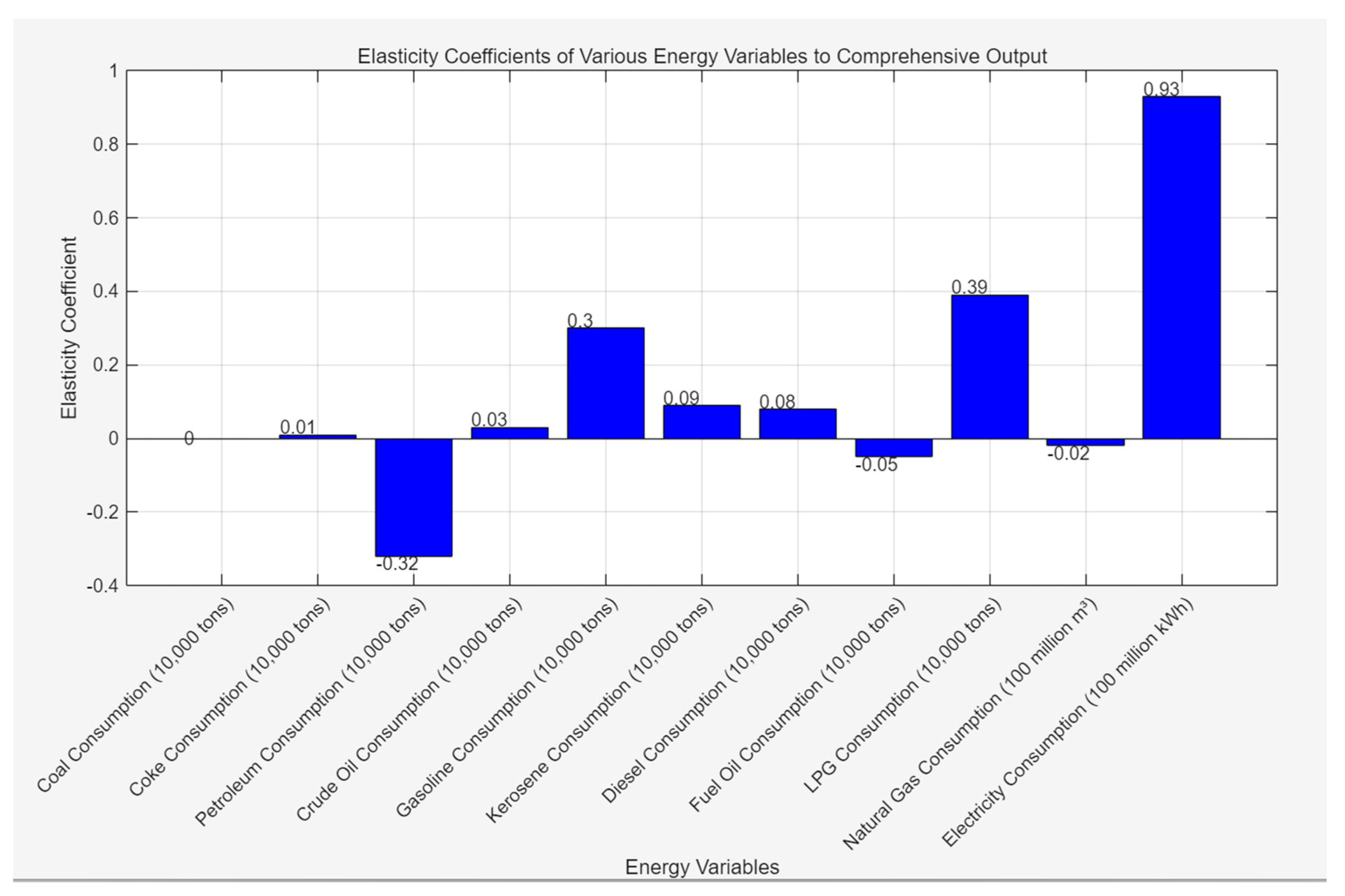
Based on LSTM 2025 forecast data, stochastic frontier analysis was conducted, and the results are shown in Figure 16 and Table A7.
From these elasticity coefficients, the impact of different energy consumption levels on the technical efficiency of population and GDP can be inferred.
Among energy sources with positive impacts:
The elasticity coefficient of electricity consumption is 0.928292, indicating that the increase in electricity consumption has a very significant positive impact on the comprehensive output of population and GDP. This is because electricity is a widely used energy source in the modern economy and social life—almost all industries rely on electricity, and sufficient and stable electricity supply helps to promote the development of production activities, drive economic growth, and further exert a positive effect on population development (e.g., increased employment opportunities attract population inflow).
The elasticity coefficient of LPG consumption is 0.392344, indicating that its increase can also promote the improvement of comprehensive output. LPG is widely used in residents’ daily life and small-scale commercial activities; the increase in its consumption may reflect the improvement of living standards and the prosperity of commercial activities, thereby having a positive impact on population and GDP.
The elasticity coefficient of gasoline consumption is 0.296263. Gasoline is mainly used in the transportation sector, especially for vehicles such as automobiles. The increase in gasoline consumption may indicate higher activity in transportation, which promotes the circulation of goods and the movement of people, facilitating economic development and population interaction, and thus having a positive effect on comprehensive output.
Among energy sources with negative impacts:
The elasticity coefficient of oil consumption is −0.319667. This negative impact may be due to the fact that oil is used more in high energy consumption and low efficiency industries, or there is waste and irrational use in oil utilization methods. As a result, the increase in oil consumption does not bring corresponding output growth and may even have a negative impact on comprehensive output due to inefficient resource allocation.
The elasticity coefficient of fuel oil consumption is −0.052826. Fuel oil is usually used in industrial boilers, power generation, and other fields. Its negative impact may imply backward technology and aging equipment in scenarios where fuel oil is used, meaning fuel oil consumption may fail to be effectively converted into driving forces for economic growth and population development.
The elasticity coefficient of natural gas consumption is −0.023922. Although the value is relatively small, it still shows a negative impact. This may be related to the supply structure and utilization efficiency of natural gas—for example, there is loss in the allocation and use of natural gas in some regions, or the industrial structure of natural gas use is irrational, failing to give full play to its role in promoting the economy and population.
The elasticity coefficient of coal consumption is −0.001858. As a traditional energy source, coal may have high pollution and high energy consumption characteristics in some regions, and backward mining and utilization technologies mean the increase in coal consumption has an insignificant or even negative effect on the improvement of comprehensive output.
The consumption elasticity coefficients of oil and fuel oil stand at −0.319667 and −0.052826, respectively, a result that carries profound warning implications from an economic perspective. Rather than denying the fundamental role of oil and fuel oil in the modern economy, it reveals severe efficiency losses and structural mismatches in the utilization of these two energy categories in some provincial regions.
From an efficiency standpoint, negative elasticity signifies that the increased input of these two energy sources has failed to generate corresponding output expansion, reflecting technological backwardness in their application links. High energy consumption of obsolete equipment, losses in processing and conversion, and waste in end-use consumption have all led to massive ineffective energy dissipation, which has not been effectively translated into a driving force for economic growth.
At a deeper level, this phenomenon is closely tied to the lock-in effect of high-carbon industries in certain regions: long-term dependence on upstream industries such as petrochemicals and iron and steel smelting, paired with short industrial chains and low value added, has caused a rapid decline in the marginal output of energy input. Typical industries including iron and steel in Hebei, the coal chemical industry in Inner Mongolia, and oil extraction in Xinjiang contribute to GDP while consuming enormous volumes of oil and fuel oil, yet the correlation between their economic output and energy input has deviated from the optimal ratio. In the meantime, institutional factors cannot be overlooked—long-standing energy price subsidies, lax environmental regulation, and insufficient incentives for green innovation have further amplified the negative effects.
Accordingly, the negative elasticity coefficient is not only a statistical manifestation of low energy utilization efficiency, but also a concentrated reflection of the rigidity of high-carbon industrial structures at the provincial level. Future policies should target industries and regions with intensive consumption of these two energy sources. Through technological renewal, clean substitution and industrial chain extension, energy input can be genuinely converted into high-quality growth, so as to achieve a fundamental improvement in carbon emission performance. In fact, existing research on green technology innovation and efficiency improvement, such as the exploration of ecological efficiency from the perspective of low-carbon city construction by Du et al. (2022) [40], provides important theoretical foundations and practical insights for understanding how to solve such negative elasticity dilemmas through innovation-driven approaches.

7.3. Comparative Discussion on Elasticity Coefficients of Hydrocarbons

The stochastic frontier analysis in this study reveals that different hydrocarbon fuels exhibit significant differences in their elasticity with respect to aggregate output: crude oil consumption shows a negative elasticity (−0.319667), whereas gasoline (0.296263) and liquefied petroleum gas (LPG, 0.392344) present positive contributions. Such divergence indicates that the consumption pattern of hydrocarbons is closely linked to their economic benefits, and existing studies provide important references for understanding this phenomenon.
Using a carbon intensity elasticity model based on input–output tables, Wang et al. [41] found that the development of 21 industrial sectors in China reduced national carbon intensity, while 7 sectors increased it during 1990–2015. For specific energy types, a 1% improvement in coal use efficiency for electricity and heat generation lowered national carbon intensity by 0.36%; a 1% rise in coke efficiency in the metal smelting and processing industry reduced carbon intensity by 0.119%; and a 1% increase in diesel efficiency in the transportation and postal industry decreased carbon intensity by 0.04%. The study also demonstrated that the carbon intensity elasticity of residential coal conservation declined significantly, while that of refined petroleum conservation rose noticeably. These findings directly support the results of the present study: the negative elasticity of crude oil may be associated with its inefficient use in coke and coal-dependent heavy industries, whereas the positive elasticity of gasoline and LPG stems from the combined effects of efficiency improvements and energy structure upgrading in sectors such as transportation.
Based on provincial panel data from 2007 to 2016, Hao et al. [42] applied the Tapio decoupling model and the Environmental Kuznets Curve (EKC) framework and confirmed an inverted U-shaped relationship between per capita GDP and carbon emissions, although the inflection point has not yet been reached. Significant disparities exist in the decoupling status across provinces, necessitating the formulation of differentiated emission reduction policies. This conclusion provides a macro background for the regional heterogeneity in this study: the negative elasticity of crude oil is likely more pronounced in heavy industry-dominated provinces with poor decoupling performance, while the positive elasticity of refined products is more evident in eastern coastal provinces with better decoupling status, verifying the necessity of differentiated strategies.
Lafati et al. [43] offered important methodological insights into research on carbon pricing and emission elasticity. Using data from 39 carbon pricing countries over 1990–2016, the study identified three key results: first, the introduction effect of carbon pricing itself can significantly reduce emissions—merely implementing carbon pricing (regardless of price level) reduces annual total emission growth by approximately 1 percentage point, with a 1.5-percentage-point drop in the electricity and heat sector; second, the marginal emission reduction effect of price levels is relatively limited—the semi-elasticity of total emissions with respect to carbon price is about −0.06% (per US dollar per ton of CO2), with statistical significance only in the manufacturing sector (−0.15%); third, ignoring the introduction effect may bias elasticity estimates, as policy implementation can shape emission behaviors by altering market expectations of future mitigation efforts. This finding suggests that the interprovincial differences in hydrocarbon elasticity observed in this study may stem not only from technical efficiency and industrial structure, but also from the timing and institutional design of provincial policies such as carbon emission trading pilots and energy taxes.
In summary, the elasticity divergence between crude oil and refined products essentially reflects the structural characteristics of hydrocarbon consumption: direct combustion of crude fuels is often tied to inefficient heavy industries, and their efficiency improvements exert a notable impact on carbon intensity (e.g., a 0.119% contribution from coke efficiency); refined products are applied in high value-added sectors such as transportation, with higher combustion efficiency and stronger value conversion capacity. Meanwhile, policy factors (e.g., the introduction effect of carbon pricing) may further moderate this relationship—this points to a direction for future research that incorporates policy variables into efficiency evaluation models.

8. Conclusions

This study constructs a multi-model integrated analytical framework featuring data preprocessing–efficiency decomposition–dynamic prediction–policy simulation. Through the systematic deconstruction and modeling of carbon emission data from 30 Chinese provinces spanning 2009 to 2019, it uncovers the profound divergent patterns of provincial carbon emission efficiency and their future evolutionary trends.
At the efficiency evaluation level, the results of data envelopment analysis (DEA) show that eastern coastal provinces and municipalities directly under the Central Government, leveraging their advantages in technological leadership and industrial structure optimization, have long occupied the efficiency frontier, with their pure technical efficiency and scale efficiency both close to or reaching the optimal level. In contrast, Hebei, Inner Mongolia, Xinjiang and other provinces with a concentration of high-carbon heavy industries are constrained by technological bottlenecks and diseconomies of scale, exhibiting prominent characteristics of efficiency depressions. Specifically, the high-carbon lock-in of Hebei’s iron and steel industry has led to a markedly low pure technical efficiency, while Inner Mongolia and Xinjiang are trapped in a structural predicament of “scale expansion outpacing efficiency improvement” due to the short industrial chains and low added value in coal, oil and gas extraction and processing.
At the trend prediction level, the simulation results of the long short-term memory (LSTM) neural network model indicate that if the share of clean energy rises to 35%, the national carbon emission growth rate is expected to drop to 1.2% by 2025. Nevertheless, a multi-scenario sensitivity analysis further reveals that the achievement of this target is highly dependent on supporting conditions such as the intensity of policy implementation and grid absorption capacity: a lag in policy implementation could cause the growth rate to rebound to 2.5%, and if the curtailment rate of wind and solar power exceeds 10%, the growth rate will also rise to 2.0%. This underscores the pivotal role of policy coherence and infrastructure coordination.
At the mechanism analysis level, the stochastic frontier model (SFM) uncovers the heterogeneous contributions of different energy types to economic and social output. The consumption elasticities of electricity, liquefied petroleum gas (LPG), and gasoline are significantly positive, reaching 0.93, 0.39 and 0.30, respectively, which attests to their high-efficiency value conversion capacity in the modern economy. In contrast, the elasticities of crude oil, fuel oil and coal are negative, at −0.32, −0.05 and −0.002, respectively, a finding that profoundly reflects the severe loss of energy utilization efficiency and rigid lock-in of high-carbon industries in some regions. Typical industries including Hebei’s iron and steel sector, Inner Mongolia’s coal chemical industry and Xinjiang’s oil extraction industry have seen their energy input and output deviate from the optimal ratio; coupled with long-standing energy price subsidies and loose environmental regulations, this has further amplified the negative effects.
Based on the above findings, this study puts forward differentiated policy pathways. For technologically backward regions, a special central–local coordinated fund for low-carbon technological transformation should be established, and the mature low-carbon technologies from eastern China should be guided to transfer and disseminate to these areas by relying on the national green technology trading platform. For regions with scale imbalance, it is necessary to shift from the simple approach of “capacity reduction” to a dual focus on “transformation and control”: while strictly curbing new capacity in high-carbon industries, leverage local renewable energy advantages to promote the extension of fossil energy industrial chains towards clean chemical manufacturing. For provinces that serve as national clean energy bases, it is imperative to revise the traditional efficiency evaluation system centered on local output and incorporate external indicators such as cross-regional green power transmission volume and carbon emission reduction contribution into the assessment system, so that the efficiency evaluation results form a positive incentive compatibility with the orientation of the national energy strategy.
Although this study has made valuable explorations in the multi-model integration method, it still has limitations such as not accounting for the offsetting effect of carbon sinks and failing to incorporate exogenous policy shocks. Future research can integrate remote sensing data (e.g., Landsat and MODIS) with ground survey data and adopt the CASA or InVEST models to estimate regional carbon sink capacity, which can then be introduced into the efficiency evaluation framework as natural capital. Meanwhile, the robustness of the model against disturbances such as extreme climate events and sudden policy changes can be enhanced through event analysis or scenario shock tests. It is expected that, in the interdisciplinary integration of Technology–Economy–Policy–Ecology, this research can contribute more forward-looking and operable scientific solutions to the low-carbon transition of China and high-carbon-dependent regions worldwide.

Author Contributions

Conceptualization, methodology, supervision, project administration, writing—review and editing, X.S.; conceptualization, methodology, supervision, writing—review and editing, Z.L.; resources, validation, B.Y.; investigation, data curation, visualization, S.L.; investigation, data curation, writing—original draft preparation, H.R.; investigation, data curation, writing—original draft preparation, visualization, K.L. All authors have read and agreed to the published version of the manuscript.

Funding

This research is supported by the Doctoral Research Fund Project of Shandong Jianzhu University (No. X25152).

Institutional Review Board Statement

Not applicable.

Informed Consent Statement

Not applicable.

Data Availability Statement

The original data presented in the study are openly available in China Statistical Yearbook and Blue Map at [35,36].

Acknowledgments

We would like to sincerely thank the teachers and students of the School of Traffic Engineering, Shandong Jianzhu University, for their strong support and generous help for this research.

Conflicts of Interest

The author Baofu Yu was employed by Shandong Taihe Urban Construction Development Co., Ltd. The remaining authors declare that the research was conducted in the absence of any commercial or financial relationships that could be construed as a potential conflict of interest.

Appendix A

Table A1. 2019 model efficiency scores of provinces in Southwest and Northwest China.
ProvinceBCC Efficiency ScoreCCR Efficiency ScoreScale Efficiency Score
Sichuan111
Yunnan0.93330.89630.9603
Gansu111
Qinghai100
Guizhou111
Chongqing111
Xinjiang10.81620.867
Ningxia111
Table A2. 2019 model efficiency scores of provinces in Central China, South China, and Northeast China.
ProvinceBCC Efficiency ScoreCCR Efficiency ScoreScale Efficiency Score
Guangdong111.0088
Hubei0.93860.93710.9983
Hunan111
Hainan111
Guangxi111
Liaoning0.534710.9456
Heilongjiang111
Jilin111
Table A3. 2019 model efficiency scores of provinces in North China and East China.
ProvinceBCC Efficiency ScoreCCR Efficiency ScoreScale Efficiency Score
Shandong111
Zhejiang111
Jiangsu111
Fujian111
Jiangxi111
Anhui111
Henan111
Hebei111
Shaanxi111
Shanxi111
Beijing111
Shanghai111
Tianjin10.91130.9113
Inner Mongolia0.98180.84640.8162
Table A4. 2025 model efficiency scores of provinces in Southwest and Northwest China.
ProvinceBCC Efficiency ScoreCCR Efficiency ScoreScale Efficiency Score
Sichuan0.992711
Yunnan0.93330.89630.9603
Gansu111
Qinghai100
Guizhou111
Chongqing111
Xinjiang10.81620.8567
Ningxia111
Table A5. 2025 model efficiency scores of provinces in Central China, South China, and Northeast China.
ProvinceBCC Efficiency ScoreCCR Efficiency ScoreScale Efficiency Score
Guangdong0.991311
Hubei0.93860.93710.9983
Hunan111
Hainan111
Guangxi111
Liaoning0.53470.50560.9456
Heilongjiang111
Jilin111
Table A6. 2025 model efficiency scores of provinces in North China and East China.
ProvinceBCC Efficiency ScoreCCR Efficiency ScoreScale Efficiency Score
Shandong111
Zhejiang111
Jiangsu111
Fujian111
Jiangxi111
Anhui111
Henan111
Hebei111
Shaanxi111
Shanxi111
Beijing111
Shanghai111
Tianjin10.91130.9113
Inner Mongolia0.98180.84640.8162
Table A7. Energy variables and elasticity coefficients.
Energy VariableElasticity CoefficientEnergy VariableElasticity Coefficient
Coal consumption (10,000 tons)−0.00186Kerosene consumption (10,000 tons)0.088925
Coke consumption (10,000 tons)0.010503Diesel consumption (10,000 tons)0.07776
Oil consumption (10,000 tons)−0.31967Fuel oil consumption (10,000 tons)−0.05283
Crude oil consumption (10,000 tons)0.025085LPG consumption (10,000 tons)0.392344
Gasoline consumption (10,000 tons)0.296263Natural gas consumption (100 million m3)−0.02392
Electricity consumption0.928292--

References

  1. Chen, G.; Qi, S.J.; Zhang, Y.B.; Wen, R.K.; Lu, Q.Q.; Wang, Y.B. Evaluation of carbon emission efficiency in construction industry based on generalized data envelopment analysis. Ecol. Econ. 2017, 33, 1–6. [Google Scholar]
  2. Zhang, C.Y. Research on Carbon Emission Calculation of Shandong Jianzhu University. Master’s Thesis, Shandong Jianzhu University, Jinan, China, 2016. [Google Scholar]
  3. Charnes, A.; Cooper, W.W.; Rhodes, E. Measuring the efficiency of decision making units. Eur. J. Oper. Res. 1978, 2, 429–444. [Google Scholar] [CrossRef]
  4. Song, X.; Xu, Y. China’s provincial low-carbon efficiency: A DEA-SBM and Malmquist analysis. Environ. Res. Commun. 2025, 7, 095014. [Google Scholar] [CrossRef]
  5. Jin, C.; Sun, Y.; Zhao, H. An analysis of low-carbon economy efficiency in 30 provinces of China based on the multi-directional efficiency method. Sustainability 2025, 17, 8045. [Google Scholar] [CrossRef]
  6. Mei, J. Evaluation of the development efficiency of China’s regional low-carbon economy based on three-stage DEA model. Front. Bus. Econ. Manag. 2022, 5, 71–77. [Google Scholar] [CrossRef]
  7. Chen, Y.; Liu, B.; Shen, Y.; Wang, X. The energy efficiency of China’s regional construction industry based on the three-stage DEA model and the DEA-DA model. KSCE J. Civ. Eng. 2016, 20, 34–47. [Google Scholar] [CrossRef]
  8. Niu, H.; Zhang, Z.; Xiao, Y.; Luo, M.; Chen, Y. A study of carbon emission efficiency in Chinese provinces based on a three-stage SBM-Undesirable model and an LSTM model. Int. J. Environ. Res. Public Health 2022, 19, 5395. [Google Scholar] [CrossRef]
  9. Chen, Y.; Ma, L.; Zhu, Z. The environmental-adjusted energy efficiency of China’s construction industry: A three-stage undesirable SBM-DEA model. Environ. Sci. Pollut. Res. 2021, 28, 58442–58455. [Google Scholar] [CrossRef]
  10. Wang, K.; Wei, Y.M.; Zhang, X. Energy and emissions efficiency patterns of Chinese regions: A multi-directional efficiency analysis. Appl. Energy 2013, 104, 105–116. [Google Scholar] [CrossRef]
  11. Guo, J.H. The efficiency evaluation of low carbon economic performance based on dynamic TOPSIS method. J. Interdiscip. Math. 2017, 20, 231–241. [Google Scholar] [CrossRef]
  12. Shi, P.; Zhang, Y.; Meng, Y.; Xu, X.; Hao, J.; Hong, F. A novel DEA-Tobit-SD assessment framework and application of provincial-level carbon emission embracing regional heterogeneity. Carbon Neutrality 2025, 4, 3. [Google Scholar] [CrossRef]
  13. Zhou, D.; Zhang, X.; Wang, X. Research on coupling degree and coupling path between China’s carbon emission efficiency and industrial structure upgrading. Environ. Sci. Pollut. Res. 2020, 27, 25149–25162. [Google Scholar] [CrossRef]
  14. Wang, D.; He, W.; Shi, R. How to achieve the dual-control targets of China’s CO2 emission reduction in 2030? Future trends and prospective decomposition. J. Clean. Prod. 2019, 213, 1251–1263. [Google Scholar] [CrossRef]
  15. Song, M.; Song, Y.; Yu, H.; Wang, Z. Calculation of China’s environmental efficiency and relevant hierarchical cluster analysis from the perspective of regional differences. Math. Comput. Model. 2013, 58, 1084–1094. [Google Scholar] [CrossRef]
  16. Yang, G.; Gui, Q.; Supanyo, P.; Zhang, F.; Yang, X.; Gong, G. Temporal and spatial changes and influencing factors of low-carbon economy efficiency in China. Environ. Monit. Assess. 2022, 195, 55. [Google Scholar] [CrossRef] [PubMed]
  17. Meng, M.; Fu, Y.; Wang, L. Low-carbon economy efficiency analysis of China’s provinces based on a range-adjusted measure and data envelopment analysis model. J. Clean. Prod. 2018, 199, 643–650. [Google Scholar] [CrossRef]
  18. Sun, W.; Chen, Y.B.; Lin, X.Y. Analysis of provincial carbon emission driving mechanisms based on the LMDI and K-means clustering method. Huanjing Kexue 2025, 46, 6142–6151. [Google Scholar]
  19. Han, Z.; Cui, B.; Xu, L.; Wang, J.; Guo, Z. Coupling LSTM and CNN neural networks for accurate carbon emission prediction in 30 Chinese provinces. Sustainability 2023, 15, 13934. [Google Scholar] [CrossRef]
  20. Wu, X.; Chen, L.; Zhao, J.; He, M.; Han, X. CNN-GRU-Attention neural networks for carbon emission prediction of transportation in Jiangsu Province. Sustainability 2024, 16, 8553. [Google Scholar] [CrossRef]
  21. Hong, S.; Fu, T.; Dai, M. Machine learning-based carbon emission predictions and customized reduction strategies for 30 Chinese provinces. Sustainability 2025, 17, 1786. [Google Scholar] [CrossRef]
  22. Jiang, X. Prediction method of carbon emissions of intelligent buildings based on secondary decomposition BAS-LSTM. Clean Technol. Environ. Policy 2024, 27, 1903–1913. [Google Scholar] [CrossRef]
  23. Chen, J.; Yang, L.H.; Ye, F.F.; Wang, Y.M. Analyzing carbon emission reduction paths in China using interpretable machine learning: A perspective of carbon emission prediction and efficiency evaluation. Environ. Dev. Sustain. 2025. [Google Scholar] [CrossRef]
  24. Luo, H.; Wang, C.; Li, C.; Meng, X.; Yang, X.; Tan, Q. Multi-scale carbon emission characterization and prediction based on land use and interpretable machine learning model: A case study of the Yangtze River Delta Region, China. Appl. Energy 2024, 360, 122819. [Google Scholar] [CrossRef]
  25. Ming, X.; Wang, Q.; Luo, K.; Zhang, X.; Fan, J. Multi-scenario carbon emission forecasting through boosting-assisted logarithmic mean divisia index and low emission analysis platform in Zhejiang, China. J. Clean. Prod. 2025, 537, 147202. [Google Scholar] [CrossRef]
  26. Li, X.; Lin, C.; Lin, M.; Jim, C.Y. Drivers, scenario prediction and policy simulation of the carbon emission system in Fujian Province (China). J. Clean. Prod. 2024, 434, 140375. [Google Scholar] [CrossRef]
  27. Gao, Z.; Xia, E.; Lin, S.; Xu, J.; Tao, C.; Yu, C. Carbon emission efficiency and regional synergistic peaking strategies in Beijing-Tianjin-Hebei region. Carbon Neutrality 2024, 3, 19. [Google Scholar] [CrossRef]
  28. Li, S.; Yao, L.; Zhang, Y.; Zhao, Y.; Sun, L. China’s provincial carbon emission driving factors analysis and scenario forecasting. Environ. Sustain. Indic. 2024, 22, 100390. [Google Scholar] [CrossRef]
  29. Xu, H.; Ren, D.; Tian, Y.; Zhang, X.; Zhang, S.; Chen, Y.; Gong, X. Exploring regional carbon emission factors and peak prediction: A case study of Hubei Province. Sustainability 2025, 18, 329. [Google Scholar] [CrossRef]
  30. Zhao, J.; Zhang, H.; Zhang, Y.; Cheng, A. Advancing China’s dual carbon goals: Regional classification and customized emission reduction strategies. Environ. Dev. Sustain. 2025. [Google Scholar] [CrossRef]
  31. Zhang, W.; Wu, X.; Chen, J. Low-carbon efficiency analysis of rail-water multimodal transport based on cross efficiency network DEA approach. Energy 2024, 305, 132348. [Google Scholar] [CrossRef]
  32. Zhu, J. DEA under big data: Data enabled analytics and network data envelopment analysis. Ann. Oper. Res. 2020, 309, 761–783. [Google Scholar] [CrossRef]
  33. Afzal, S.; Ziapour, B.M.; Shokri, A.; Shakibi, H.; Sobhani, B. Building energy consumption prediction using multilayer perceptron neural network-assisted models; comparison of different optimization algorithms. Energy 2023, 282, 128446. [Google Scholar] [CrossRef]
  34. Wang, M.; Lu, N.; Liu, L.; Chen, L.; Li, X. Research on driving factors and efficiency measures of low-carbon levels in less-developed regions: A case of Western China. Greenh. Gases Sci. Technol. 2024, 14, 526–545. [Google Scholar] [CrossRef]
  35. National Bureau of Statistics of China. China Statistical Yearbook 2020; China Statistics Press: Beijing, China, 2020. [Google Scholar]
  36. Institute of Public and Environmental Affairs (IPE). Blue Map. Available online: http://wwwtestweb.ipe.org.cn:8099/index.html (accessed on 6 August 2025).
  37. Banker, R.D.; Charnes, A.; Cooper, W.W. Some Models for Estimating Technical and Scale Inefficiencies in Data Envelopment Analysis. Manag. Sci. 1984, 30, 1031–1142. [Google Scholar] [CrossRef]
  38. Hochreiter, S.; Schmidhuber, J. Long Short-Term Memory. Neural Comput. 1997, 9, 1735–1780. [Google Scholar] [CrossRef] [PubMed]
  39. Aigner, D.; Lovell, C.A.K.; Schmidt, P. Formulation and estimation of stochastic frontier production function models. J. Econ. 1977, 6, 21–37. [Google Scholar] [CrossRef]
  40. Du, M.; Antunes, J.; Wanke, P.; Chen, Z. Ecological efficiency assessment under the construction of low-carbon city: A perspective of green technology innovation. J. Environ. Plan. Manag. 2022, 65, 1727–1752. [Google Scholar] [CrossRef]
  41. Wang, F.; Sun, X.; Reiner, D.M.; Wu, M. Changing trends of the elasticity of China’s carbon emission intensity to industry structure and energy efficiency. Energy Econ. 2020, 86, 104679. [Google Scholar] [CrossRef]
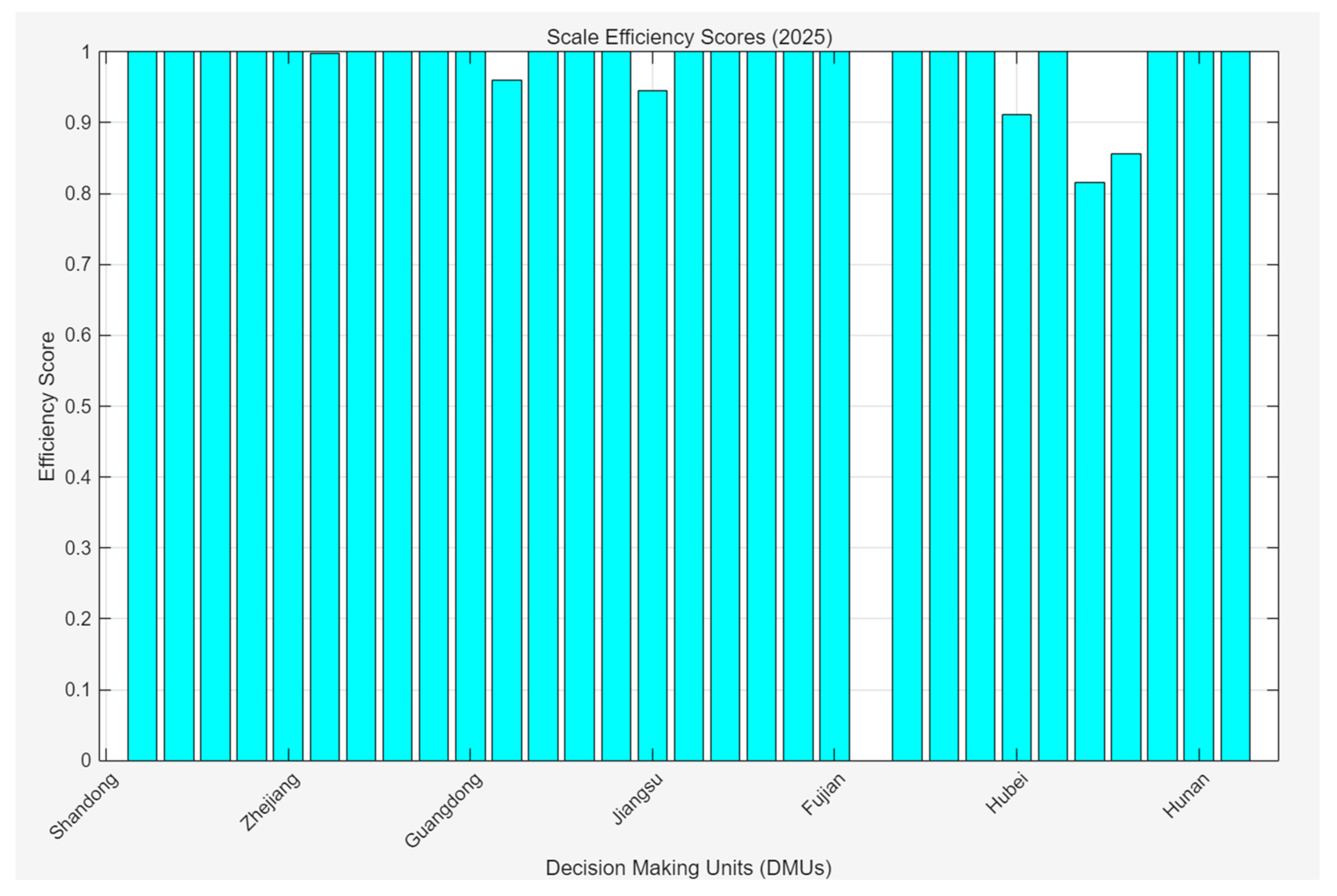
  42. Hao, Y.; Huang, Z.; Wu, H. Do carbon emissions and economic growth decouple in China? An empirical analysis based on provincial panel data. Energies 2019, 12, 2411. [Google Scholar] [CrossRef]
  43. Lafati, R.; Dolphin, J.; Press, F. Carbon pricing and the elasticity of carbon monoxide emissions. Energy Econ. 2025, 144, 108298. [Google Scholar] [CrossRef]
Figure 1. Research content roadmap.
Sustainability 18 02545 g001
Figure 2. Schematic diagram of IQR outlier identification.
Sustainability 18 02545 g002
Figure 3. Total carbon emissions of provinces in North China and East China (×1013 tC).
Sustainability 18 02545 g003
Figure 4. Total carbon emissions of provinces in Northeast China.
Sustainability 18 02545 g004
Figure 5. Total carbon emissions of provinces in Northwest and Southwest China (×1013 tC).
Sustainability 18 02545 g005
Figure 6. Total carbon emissions of provinces in Central China and South China.
Sustainability 18 02545 g006
Figure 7. Residual plot of provincial indicators versus the average.
Sustainability 18 02545 g007
Figure 8. Bar chart of BCC efficiency scores (2019).
Sustainability 18 02545 g008
Figure 9. Bar chart of CCR efficiency scores (2019).
Sustainability 18 02545 g009
Figure 10. Bar chart of scale efficiency scores (2019).
Sustainability 18 02545 g010
Figure 11. Comparison between predicted and actual values of various resource consumption (Shandong Province, 2009–2025).
Sustainability 18 02545 g011
Figure 12. Sensitivity analysis of 2025 carbon emission growth rate across scenarios.
Sustainability 18 02545 g012
Figure 13. Bar chart of BCC efficiency scores (2025).
Sustainability 18 02545 g013
Figure 14. Bar chart of CCR efficiency scores (2025).
Sustainability 18 02545 g014
Figure 15. Bar chart of scale efficiency scores (2025).
Sustainability 18 02545 g015
Figure 16. Elasticity coefficients of various energy variables on comprehensive output.
Sustainability 18 02545 g016
Table 1. Conversion standards for various fuel data.
CategoryFuel TypeHeating Value (TJ)Carbon Content per Unit Calorific Value (tC/TJ)
Solid fuelAnthracite2.93 × 10727.4
Coke2.93 × 10729.5
Liquid fuelPetroleum84020
Crude oil84020.1
Kerosene2.93 × 10719
Fuel oil41.81621.1
Gasoline4.27 × 10718.9
Diesel oil42.55220.2
Liquefied petroleum gas (LPG)50.17917.2
Natural gas3.75 × 10417.2
ElectricityElectricity3600 (kJ/kWh)16 (kC/kWh)
Table 2. Total carbon emissions of provincial-level regions in China.
Region CategoryProvinceTotal Carbon Emissions (×1013 tC)
North China and East ChinaShandong Province79,800
Jiangsu Province68,500
Guangdong Province67,200
Zhejiang Province52,300
Henan Province51,800
Beijing Municipality12,600
Tianjin Municipality9800
Northeast ChinaLiaoning Province32,400
Heilongjiang Province21,700
Jilin Province10,300
Northwest and Southwest ChinaXinjiang Uygur Autonomous Region39,600
Sichuan Province24,800
Guizhou Province19,700
Yunnan Province18,500
Ningxia Hui Autonomous Region16,200
Gansu Province15,800
Chongqing Municipality14,300
Qinghai Province4900
Central China and South ChinaHubei Province29,600
Hunan Province20,300
Guangxi Zhuang Autonomous Region19,800
Jiangxi Province17,400
Hainan Province3200
Disclaimer/Publisher’s Note: The statements, opinions and data contained in all publications are solely those of the individual author(s) and contributor(s) and not of MDPI and/or the editor(s). MDPI and/or the editor(s) disclaim responsibility for any injury to people or property resulting from any ideas, methods, instructions or products referred to in the content.