


Abstract
Accurate prediction of wheat prices is crucial for market participants and policymakers because volatility in agricultural markets affects food security and economic planning. This study proposes a hybrid deep-learning-based framework for daily wheat price prediction in Türkiye. The approach first applies an autoencoder to detect and remove anomalous price–quality records from a dataset of 38,019 market transactions collected between June 2022 and May 2023. A weighted ensemble combining Linear Regression, Random Forest, Support Vector Regression and an attention-based Long Short-Term Memory network is then trained on quality parameters and market attributes, with data split into training, validation and test sets. On the independent test set the ensemble achieved a coefficient of determination R2 = 0.9942 and a mean absolute error of 0.1646 TL, outperforming the constituent models. SHAP analysis identifies the price–quality ratio as the most influential feature, while the ablation analysis shows that some of the high accuracy derives from price-derived variables’ strong correlation with the target. Cross-validation confirms robustness and generalization. Overall, the framework provides an effective and interpretable tool for wheat price forecasting, though the short data collection period and single-product focus limit generalizability.
1. Introduction
Agricultural product price prediction plays a crucial role for market participants, policymakers, and farmers, particularly for strategic grain products such as wheat. Price fluctuations in wheat markets have far-reaching implications for food security, economic stability, and long-term agricultural planning. These fluctuations are driven by a wide range of interacting factors, including weather variability, changes in market demand, and global trade dynamics [1]. Due to the nonlinear and highly volatile nature of these interactions, traditional statistical prediction approaches often fail to provide satisfactory predictive performance, whereas machine learning and deep learning techniques have demonstrated superior capabilities in modeling such complex relationships.
Among deep learning models, Long Short-Term Memory (LSTM) networks have been extensively applied to time series prediction problems owing to their ability to capture long-term dependencies in sequential data [2]. The integration of attention mechanisms into LSTM architectures has further enhanced prediction accuracy by allowing models to focus on the most informative time steps within a sequence [3,4]. In agricultural applications, LSTM-based models have achieved notable success in wheat yield prediction [5] and agricultural commodity price prediction [6]. Attention-based LSTM models have improved prediction performance by emphasizing critical temporal patterns in price series [7]. Gu et al. (2022) proposed a dual-input attention LSTM model incorporating both feature-level and temporal attention mechanisms, integrating meteorological variables, trading volume, and price data, and achieved a mean absolute percentage error of approximately 3.26% [8].
Ensemble learning methods aim to improve generalization performance by combining the predictions of multiple base models. Weighted ensemble approaches assign higher importance to more accurate or reliable models, thereby enhancing overall prediction robustness [9]. Random Forest algorithms provide stable and robust predictions through the aggregation of multiple decision trees [10], while Support Vector Regression (SVR) is well suited for capturing nonlinear relationships in regression problems [11]. In agricultural prediction, ensemble techniques have consistently outperformed single-model approaches by mitigating individual model limitations [12]. For instance, Celik and Celik (2025) proposed a hybrid framework combining LSTM, Autoregressive Integrated Moving Average (ARIMA), Vector Autoregression (VAR), and stochastic models to forecast agricultural commodity prices, demonstrating the superiority of LSTM in capturing nonlinear dynamics [13]. Similarly, Choudhary et al. (2025) showed that integrating Variational Mode Decomposition (VMD) optimized by a genetic algorithm with LSTM significantly reduced prediction errors in corn price prediction [14].
Beyond predictive accuracy, data quality and anomaly detection are critical considerations in real-world agricultural prediction systems. Autoencoder architectures have emerged as effective tools for identifying abnormal patterns, erroneous measurements, and unexpected events, particularly in agricultural sensor and market data [15,16]. By detecting patterns not observed during training, autoencoder-based approaches contribute to improved data reliability and prediction robustness [17,18,19].
Autoencoders are unsupervised neural networks that learn to reconstruct input data through a compressed bottleneck representation. By forcing the network to pass information through a low-dimensional latent space, autoencoders learn latent features that highlight unusual or poorly represented patterns [20]. In agricultural applications, stacked and variational autoencoders have been employed to identify sensor noise, misrecorded values and outliers, thereby enhancing data reliability before forecasting [15].
Interpretability is a critical requirement for the practical adoption of machine learning and deep learning models, particularly in data-driven decision-making contexts. SHapley Additive exPlanations (SHAP) offer a theoretically grounded and model-agnostic framework for quantifying the contribution of each input feature to a model’s predictions. Rooted in cooperative game theory, SHAP decomposes an individual prediction into a sum of additive feature attributions, where each SHAP value represents a feature’s marginal contribution averaged over all possible feature subsets. This formulation guarantees desirable properties such as local accuracy, consistency, and missingness invariance, regardless of the underlying model architecture. By revealing the key drivers behind price predictions at both global and instance levels, SHAP enhances model transparency, enabling domain experts to better understand, validate, and trust complex machine learning and deep learning outputs, while also supporting tasks such as model debugging and effective communication of results to stakeholders [21].
Deep learning techniques have been increasingly adopted in agricultural prediction due to their ability to automatically extract meaningful features from large and complex datasets [22,23]. Empirical studies in wheat yield estimation [12,24,25] and agricultural commodity price prediction [1,25] consistently demonstrate that deep learning models often outperform traditional machine learning approaches in terms of predictive accuracy. However, these performance gains are frequently achieved at the cost of reduced generalization capability, higher sensitivity to data quality, and increased risk of overfitting when relying on a single model architecture. Moreover, single-model frameworks typically struggle to simultaneously ensure robustness, interpretability, and stability across heterogeneous data conditions. To address these limitations, hybrid frameworks that integrate deep learning and machine learning models have emerged as a more reliable paradigm, as they enable the complementary strengths of different model classes to be combined, thereby improving robustness, generalization performance, and practical reliability in real-world agricultural forecasting applications.
In this study, we treat machine learning models (e.g., Linear Regression, Random Forest and SVR) and deep learning models (e.g., LSTM equipped with attention mechanisms) as complementary components. Machine-learning algorithms provide fast, interpretable predictions on tabular agricultural data, while deep-learning architectures excel at capturing nonlinear temporal dynamics. Ensemble learning combines these heterogeneous models to harness their respective strengths, improving prediction performance and robustness [2,10,26,27,28].
Recent literature underscores both the promise and limitations of hybrid deep-learning approaches for agricultural price prediction. A systematic review of machine-learning methods for staple crops such as wheat, corn and rice highlights that hybrid deep-learning models generally outperform traditional algorithms but often suffer from poor interpretability and a heavy reliance on region-specific or short-term datasets. The authors note that the absence of explainable components and limited generalizability across regions constrain the practical use of these models [29].
Several studies report impressive accuracy gains using advanced signal-decomposition and optimization techniques. For example, a Bi-DSConvLSTM-Attention model that combines bidirectional LSTM with depthwise separable convolution and an attention layer achieved R2 ≈ 0.9984 and MAPE ≈ 0.55% on grain futures, but relies on complex mutual-information-based feature selection and convolutional filters [30]. A framework combining successive variational mode decomposition (SVMD), a CNN-augmented bidirectional LSTM and a multiple strategies dung beetle optimization algorithm reduced MAPE by 25.78–37.57% compared with single models [31]. Such layered decompositions boost accuracy at the cost of computational complexity and interpretability.
Other studies explore alternative architectures and exogenous factors. A VMD-SGMD-LSTM hybrid applies variational mode decomposition and smoothed global minimum density decomposition to denoise price series before LSTM prediction; it improved forecasting ability and robustness across wheat, corn and sugar futures relative to conventional models [32]. A time-convolution network (TCN) combined with XGBoost achieved RMSE ≈ 0.26 and MAPE ≈ 5.3%, outperforming ARIMA, LSTM and Transformer-XGBoost baselines during periods of price volatility [33]. A seasonal–trend decomposition–variational mode decomposition–particle swarm optimization BiLSTM model (SV-PSO-BiLSTM) achieved RMSE ≈ 0.2241, MAE ≈ 0.1665 and MAPE ≈ 0.0207 on various agricultural futures [34]. While these approaches yield very low error metrics, they depend on sophisticated preprocessing and hyperparameter tuning, limiting scalability and real-time applicability.
Despite methodological advances, most existing models treat data quality as a separate preprocessing step and rarely integrate anomaly detection or interpretability into the forecasting pipeline. Only a few studies explicitly address interpretability; for instance, an explainable Bi-LSTM model for winter wheat yield prediction uses local interpretable model-agnostic explanations (LIME), Integrated Gradient and SHAP to show that enhanced vegetation index, temperature and precipitation are the dominant drivers, but reports R2 ≈ 0.88 and does not embed explainability within an ensemble framework [35]. Likewise, a hybrid Prophet model that tunes seasonality parameters and augments forecasts with gradient boosting improves MAE, RMSE and MAPE compared with baseline Prophet models but still lacks fine-grained explanations of feature contributions [36]. These findings illustrate that while current models achieve respectable predictive performance, they often overlook coordinated treatment of data quality control, predictive accuracy and interpretability. Addressing these gaps requires integrating anomaly detection and explainability within the modeling architecture without relying on complex decompositions or external data sources.
Despite the significant progress achieved in agricultural price prediction through deep learning and ensemble-based approaches, several critical gaps remain in the existing literature. Most prior studies primarily focus on improving predictive accuracy, while overlooking the combined challenges of data quality assurance, anomaly detection, and model interpretability within a unified prediction framework. Anomaly detection is often treated as a preprocessing step or entirely neglected, and interpretability analyses are rarely integrated with ensemble-based deep learning models in agricultural price prediction studies. Moreover, many existing models rely on either complex data decomposition techniques or extensive external datasets, which may limit their practical applicability and scalability in real market environments. To address these limitations, this study proposes an integrated hybrid deep learning framework that simultaneously integrates attention-based LSTM prediction, autoencoder-driven anomaly detection, and weighted ensemble learning, complemented by SHAP-based model interpretability. By jointly addressing accuracy, robustness, and transparency within a single system and by validating the approach on real-world Turkish wheat market data, this study contributes a practical, interpretable, and high-performance solution to agricultural price prediction, thereby advancing both methodological research and decision-support applications in agricultural markets.
The main research question of this study is: Can a reliable, interpretable price prediction system that includes anomaly detection be developed for the Turkish wheat market using quality parameters and market characteristics? To answer this question, the following research tasks were carried out in the study: Developing a weighted ensemble prediction framework integrating attention-mechanism LSTM, Linear Regression, Random Forest, and SVR models; ensuring data quality control with autoencoder-based anomaly detection; enhancing the interpretability of model decisions with SHAP analysis; and validating the proposed framework with real data obtained from the Turkish wheat market.
This study contributes to the existing literature by presenting an integrated approach that combines anomaly detection, price prediction, and interpretability components within a single framework, as the simultaneous integration of these three components has rarely been addressed in the literature. Furthermore, high prediction performance is achieved without requiring complex signal decomposition techniques or extensive external data sources, while SHAP-based interpretability analysis provides a systematic framework for model transparency in agricultural price forecasting.
In terms of the practical application potential of the proposed framework, farmers can benefit from this system in their harvest and sales timing decisions, market participants in their buying and selling strategies, and policymakers in planning agricultural support policies. Autoencoder-based anomaly detection enables the identification of erroneous or inconsistent records in corporate data sources, while SHAP analysis allows decision-makers to understand the factors behind predictions.
2. Materials and Methods
2.1. Dataset and Preprocessing
The dataset used in this study consists of 38,019 records and 23 features collected from Türkiye’s agricultural products market between 1 June 2022 and 4 May 2023. The data were obtained from the Konya Branch of the Turkish Grain Board (Toprak Mahsulleri Ofisi, TMO, Ankara, Turkey), a governmental institution responsible for grain procurement, quality assessment, and market regulation in Türkiye. The Konya Branch compiles daily transaction records reflecting actual market operations, including price information and detailed quality inspection results. The dataset includes quality-related parameters such as moisture, hectoliter weight, protein content, defective grains, broken grains, shriveled grains, foreign matter, and husk, together with market-related attributes including unit price, estimated quantity, transaction date, product class, and product type. All feature labels and categorical variables are provided in the Turkish language, reflecting the original structure of the institutional data source.
To ensure robust model evaluation and to prevent overfitting, the dataset was partitioned into training (60%, n = 22,811), validation (20%, n = 7604), and test (20%, n = 7604) subsets. The test set was strictly excluded from the model training process and was used only for final performance assessment.
Overall data quality was high, with missing values observed only in the ClassName attribute, accounting for 2.43% of the total records. Based on the original 23 features, eight additional variables were derived through feature engineering to enhance predictive capability, including the price–quality ratio, quality score, 7-day price moving average, price trend, total defect ratio, seasonal indicator, week number, and price volatility. In addition, categorical variables (product class and product type) were label-encoded, and temporal features (month, day) were extracted from the transaction date as part of standard preprocessing.
The additional variables were computed as follows: (i) Price–quality ratio: the unit price divided by the quality score; (ii) Quality score: a weighted composite index derived from moisture, hectoliter weight, and protein content, with penalties for total defect ratio, normalized to the [0, 1] interval; (iii) Price trend: the difference between the current unit price and its 7-day moving average; (iv) Total defect ratio: the sum of defective grains, broken grains, shriveled grains, foreign matter, and husk (all expressed as percentages); (v) Seasonal indicator: a binary variable equal to 1 if the transaction date falls between June and September (harvest season) and 0 otherwise; (vi) Week number: the ISO week number extracted from the transaction date; and (vii) Price volatility: the rolling standard deviation of the unit price over the preceding seven days, (viii) 7-day price moving average: the arithmetic mean of the unit price over the preceding seven days.
All numerical features were scaled using Min–Max normalization to the [0, 1] interval. Importantly, normalization parameters were computed exclusively from the training set and subsequently applied to the validation and test sets to avoid data leakage.
The target variable, unit price, ranges from 0 to 32 TL, with a mean value of 6.33 TL and a standard deviation of 2.50 TL. Estimated transaction quantities vary between 0 and 296,000 tons, with an average of 25,945 tons. The dataset comprises 103 distinct product types and 40 product classes, with corn (49.4%), barley (13.0%), and durum wheat (6.8%) being the most frequently observed commodities. To enhance data reliability, an autoencoder-based anomaly detection model was employed, identifying 390 anomalous observations (1.03%), primarily associated with zero prices, zero quantities, and logically inconsistent feature combinations.
The anomalous observations were removed from the training and validation subsets to prevent bias during model training, but they were retained in the test set for independent analysis and evaluation of the anomaly detection module.
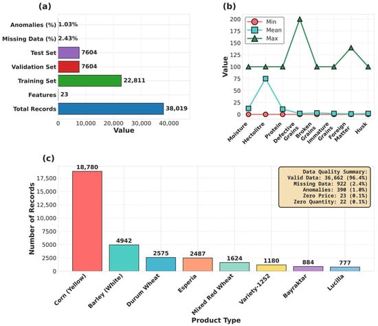
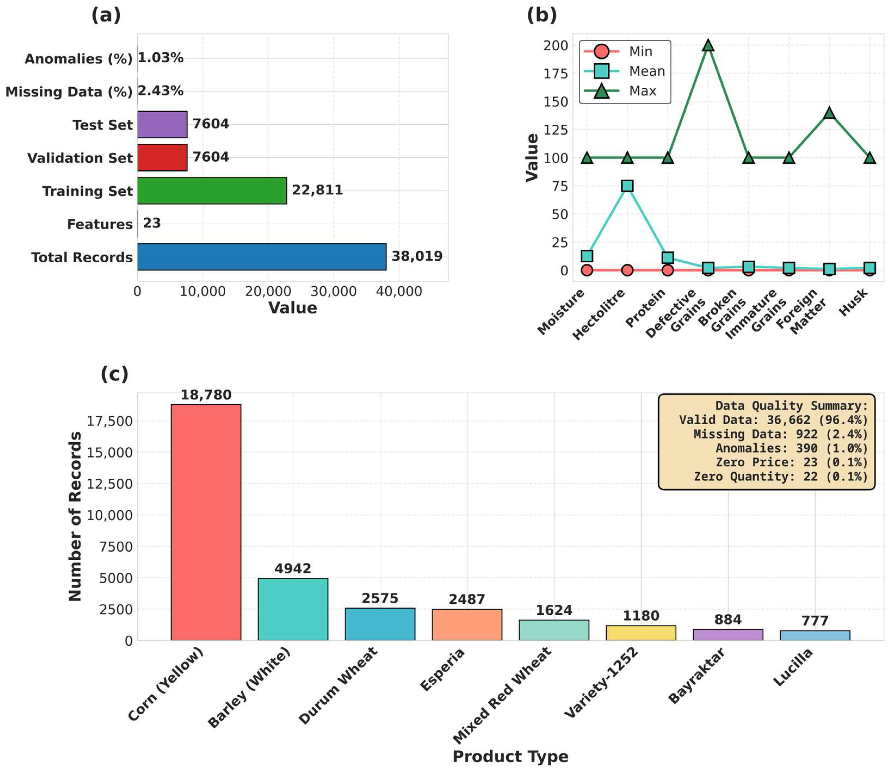
A comprehensive overview of the dataset characteristics, quality parameter distributions, and product composition is presented in Figure 1.
Figure 1.
Dataset overview and quality assessment. (a) Dataset statistics and training, validation, and test split. (b) Distribution of quality parameters in terms of minimum, mean, and maximum values. (c) Product distribution and data quality summary.
As illustrated in Figure 1a, the dataset is evenly and systematically divided into training, validation, and test subsets following a 60%–20%–20% split. Figure 1b demonstrates the wide variability observed in key quality parameters, such as protein content and defective grain ratios, highlighting their potential influence on price formation. Figure 1c shows that corn constitutes nearly half of the dataset, while the proportion of anomalous and missing records remains relatively low, confirming the overall reliability of the data used in this study.
2.2. Modeling Strategy
A hybrid modeling framework was adopted to simultaneously address wheat price prediction and anomaly detection. The proposed approach integrates the strong representation of learning capability of deep learning models, namely attention-based LSTM networks and autoencoders, with the robustness and interpretability of conventional machine learning algorithms, including Linear Regression, Random Forest, and SVR. All constituent models were trained on the same training dataset, and their outputs were subsequently combined using a weighted ensemble strategy to enhance generalization performance and robustness.
2.2.1. Predictive Modeling Module
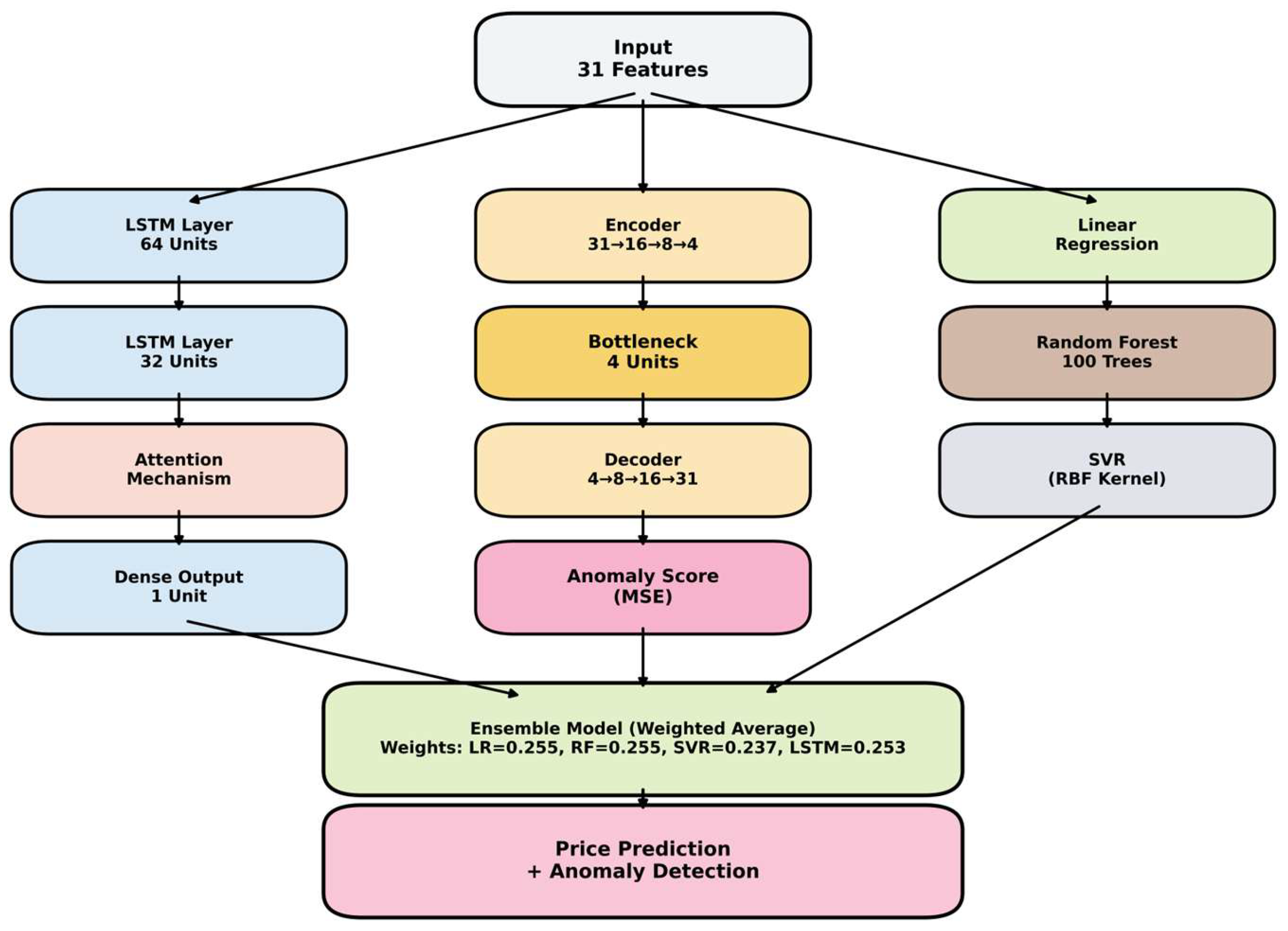
This module focuses on price prediction using both deep-learning and traditional machine-learning models. The left branch implements an attention-based LSTM architecture: a first LSTM layer with 64 units captures temporal dependencies in the input sequences, followed by a second LSTM layer with 32 units to refine temporal feature representations. An attention mechanism is then applied to emphasize the most informative time steps, and the resulting context vector is passed to a dense output layer with a single neuron to generate the price prediction. The right branch comprises three conventional regression models—Linear Regression, Random Forest with 100 trees and SVR with a radial basis function kernel—which provide complementary predictive perspectives and serve as robust baseline learners within the ensemble framework.
2.2.2. Anomaly Detection Module
The middle branch employs an autoencoder architecture to identify anomalous observations. The encoder progressively compresses the 31-dimensional input feature space into a 4-dimensional bottleneck representation through intermediate layers (31 → 16 → 8 → 4). The decoder symmetrically reconstructs the input (4 → 8 → 16 → 31), and the reconstruction error, measured using mean squared error (MSE), serves as an anomaly score. Higher reconstruction errors indicate abnormal observations, such as zero prices, zero quantities or logically inconsistent feature combinations.
2.2.3. Ensemble Integration Module
Finally, the outputs of the four predictive models—Linear Regression, Random Forest, SVR and the attention-based LSTM—are combined using a weighted average ensemble scheme. The weights were empirically determined as 0.255 for Linear Regression, 0.255 for Random Forest, 0.237 for SVR and 0.253 for LSTM. This ensemble strategy enables the system to simultaneously deliver accurate price predictions while incorporating anomaly detection results from the autoencoder module, yielding a unified and reliable decision-support output.
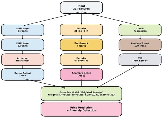
The overall architecture of the proposed hybrid framework is illustrated in Figure 2.
Figure 2.
Proposed hybrid modeling architecture for price prediction and anomaly detection.
As shown in Figure 2, the system consists of three parallel processing paths originating from a common input layer comprising 31 features.
2.3. Strategy Implementation
This section explains how each module described in Section 2.2 was implemented at the algorithmic level. Rather than presenting predictive results (which are summarized in Section 3), we focus here on the modeling pipelines, training procedures and ensemble integration logic used to build the proposed framework. All implementations were carried out in Python 3.11; deep-learning components were developed with TensorFlow 2.15/Keras 3.0, while classical machine-learning algorithms were implemented using scikit-learn 1.3.2.
2.3.1. Predictive Modeling Module Implementation
The Linear Regression baseline model was fitted using ordinary least squares. Given a set of explanatory variables and a target vector , the model solves and outputs predictions ; this was accomplished using scikit-learn’s LinearRegression class. The Random Forest model was implemented via the RandomForestRegressor class with 100 trees. Each tree was trained on a bootstrap sample of the training data, and node splits were chosen to minimize the mean squared error; final predictions were obtained by averaging predictions across all trees. The SVR model employed a radial-basis-function kernel to capture non-linear relationships. SVR solves a convex optimization problem that minimizes a combination of the -insensitive loss and a regularization term; we used scikit-learn’s SVR class with fixed hyperparameters (kernel = “rbf”, C = 100, ε = 0.05). These hyperparameter values were selected based on validation experiments and remained fixed during model training; a systematic sensitivity analysis is reported in Section 3.2. The attention-based LSTM architecture comprised two stacked LSTM layers with 64 and 32 hidden units, respectively, followed by a dense output layer. Each LSTM layer computed hidden states and cell states through gated recurrence equations, thereby capturing long-range dependencies in the input sequence. An attention mechanism was then applied over the sequence of LSTM outputs. Specifically, we computed attention weights , where and is the final hidden state. The context vector was concatenated with and passed through a fully connected layer to produce the final prediction. The network was trained using the Adam optimizer with a learning rate of 0.001 and a batch size of 64; early stopping with a patience of 10 epochs was applied based on validation loss. These training hyperparameters (two hidden layers with 64 and 32 units, learning rate 0.001, batch size 64, patience 10) were fixed for all experiments.
2.3.2. Anomaly Detection Module Implementation
The autoencoder used for anomaly detection consisted of an encoder and decoder arranged symmetrically: the encoder compressed the 31-dimensional input through hidden layers of sizes 16 and 8 into a 4-dimensional bottleneck, and the decoder reconstructed the input by expanding back through layers of sizes 8 and 16 to the original dimension. During training, the model minimized the mean squared reconstruction error between inputs and outputs. After training on the normal data, the reconstruction error served as an anomaly score for observation . Observations with errors above the 95th percentile of training reconstruction errors were flagged as anomalies and removed from the training/validation sets; the flagged observations were retained in the test set to evaluate anomaly detection performance. This anomaly threshold (95th percentile) was fixed and not tuned further.
2.3.3. Ensemble Integration Implementation
To combine the diverse predictive models, we employed a weighted averaging scheme. Let , , and denote the predictions from Linear Regression, Random Forest, SVR and LSTM-Attention, respectively. The final ensemble prediction for each sample was computed as , where the weights , , and satisfy and were determined by normalizing each model’s R2 on the validation set. Models with higher validation R2 thus received greater influence in the final prediction. The empirically determined weights (0.255 for Linear Regression, 0.255 for Random Forest, 0.237 for SVR and 0.253 for LSTM) were fixed during evaluation; alternative weighting strategies and their impact on performance are discussed in Section 3.
The prices used in the study are current (nominal) prices in Turkish Lira and reflect the current market values on the transaction date. Due to the relatively short data collection period, no inflation adjustment has been applied. Ensemble model weights have been empirically determined based on each model’s R2 performance on the validation set. The R2 value for validation was calculated for each model and normalized by dividing these values by the total R2 value. This approach ensures that models with higher prediction accuracy are given greater weight.
For reproducibility and transparency, the complete implementation, including source code, trained models, raw and preprocessed datasets, prediction outputs, anomaly detection results, figure generation scripts, training logs, and comprehensive analysis artifacts such as SHAP values and cross-validation metrics, is publicly available at https://github.com/yeldafrt/Hybrid-LSTM-Autoencoder-Model-for-Wheat-Prices (accessed on 10 February 2026).
2.4. SHAP Analysis and Model Interpretability
Beyond achieving high predictive accuracy, the practical adoption of machine learning models in agricultural commodity markets requires transparent and interpretable decision mechanisms. In this context, the SHAP 0.44.0 library was employed to enhance model interpretability by quantitatively assessing the contribution of each input feature to the price predictions generated by the proposed ensemble model. Rooted in cooperative game theory, SHAP values provide a consistent and theoretically grounded framework for explaining black-box model outputs by attributing prediction outcomes to individual features [21].
The SHAP analysis was conducted on the independent test dataset (n = 7604) and structured around three main feature categories to reflect the multi-dimensional nature of wheat price formation. The first category comprises quality parameters, including moisture content, hectoliter weight, protein ratio, defective grains, broken grains, shriveled grains, foreign matter, and husk. The second category represents market-related information, such as unit price, estimated quantity, transaction date, product class, and product type.
The SHAP results reveal that the price–quality ratio is by far the most influential feature, with an importance value of 0.9908, accounting for approximately 99.08% of the variance in the ensemble model’s predictions. This dominant contribution indicates that the interaction between quality features and pricing is the primary driver of wheat price estimation within the proposed framework. In contrast, secondary features such as the overall quality score (0.0059), price trend (0.0012), and moisture content (0.0005) exhibit relatively minor contributions to the prediction outcomes. While these features provide additional contextual information, their marginal influence suggests that they act mainly as supporting factors rather than primary determinants.
From an interpretability perspective, these findings confirm that the ensemble model relies predominantly on economically meaningful and domain-consistent relationships rather than spurious correlations. The dominance of the price–quality ratio aligns well with real-world trading practices, where quality-adjusted pricing mechanisms play a central role in wheat markets. Moreover, the SHAP-based decomposition enhances trust in the proposed model by enabling market participants and agricultural experts to trace prediction outcomes back to tangible and interpretable factors.
Overall, the SHAP analysis not only improves the transparency of the proposed hybrid framework but also provides actionable insights for traders, policymakers, and analysts. By highlighting the central role of quality-adjusted pricing, the interpretability results support data-driven decision-making and reinforce the practical relevance of the proposed approach for real-world agricultural commodity price prediction.
3. Results
3.1. Performance Evaluation
The performance of the proposed models was comprehensively evaluated using three complementary perspectives: (i) predictive accuracy on the independent test set, (ii) robustness analysis via 5-fold cross-validation, and (iii) generalization capability assessment. The comparative performance of all models on the test set is reported in Table 1, while the cross-validation and generalization analyses are summarized in Table 2 and Table 3, respectively.
Table 1.
Performance of the Test Set (External Data) for All Models.
Table 2.
5-Fold Cross-Validation Results (Train + Validation Set: N = 30,414).
Table 3.
Generalization Analysis: Train, Validation, and Test Performance.
Table 1 presents the predictive performance of the individual models and the proposed ensemble approach on the external test dataset using the coefficient of determination (R2), mean absolute error (MAE), root mean squared error (RMSE), and mean absolute percentage error (MAPE). The Linear Regression model achieves a perfect fit with an R2 value of 1 and zero error metrics. Although this result indicates exact prediction on the test set, it also suggests a potential risk of overfitting, particularly when applied to unseen data.
The Random Forest model demonstrates strong predictive capability, yielding an R2 value of 0.9995 and a low MAE of 0.0103 TL, indicating that its predictions deviate from actual prices by only 0.0103 Turkish Lira on average. The attention-based LSTM model also exhibits high performance, achieving an R2 value of 0.9912 with an MAE of 0.1782 TL, confirming its effectiveness in capturing nonlinear temporal dependencies in wheat price data. In contrast, the SVR model shows comparatively lower performance, with an R2 value of 0.9297 and an MAE of 0.5844 TL.
The proposed ensemble model, constructed using a weighted aggregation of Linear Regression, Random Forest, SVR, and LSTM with attention, delivers balanced and reliable performance across all evaluation metrics. As reported in Table 1, the ensemble achieves an R2 value of 0.9942 and an MAE of 0.1646 TL. Considering the average unit price of 6.33 TL, this corresponds to an approximate prediction error of 2.6%. By integrating multiple modeling perspectives, the ensemble approach effectively mitigates the overfitting risk observed in individual models and provides a robust solution suitable for deployment in real-world production environments.
As reported in Table 2, the Linear Regression model exhibits consistently strong performance across all cross-validation folds, achieving a mean R2 value of 1. The Random Forest model also demonstrates high and stable predictive accuracy, with a mean R2 value of 0.9972. Although a slight performance decrease is observed in Fold 4, the overall results indicate robust and reliable behavior across different data partitions. In contrast, the SVR model yields comparatively lower performance, with a mean R2 value of 0.9161. Nevertheless, the close agreement between training and testing R2 values across all models suggests satisfactory generalization capability and indicates that none of the evaluated models suffer from significant overfitting.
As summarized in Table 3, the comparative analysis of model performance across the training, validation, and test datasets indicates that none of the evaluated models exhibit significant overfitting. For the Linear Regression and Random Forest models, the training and test performances are nearly identical, with performance gaps approaching zero. In the case of the SVR model, the test performance slightly exceeds the training performance, resulting in a negative performance gap (Gap = −0.0118). This outcome suggests that the model maintains stable generalization capability when applied to unseen data.
To evaluate the models’ performance in greater depth, an ablation analysis was conducted to examine the effect of price-derived variables (Price-Quality Ratio, 7-Day Price Moving Average, Price Trend, and Price Volatility) on model performance. Since these variables contain information directly related to the target variable, unit price, their removal aims to more clearly reveal the models’ actual predictive capacity. Table 4 compares the test set performance when price-derived variables are included and excluded.
Table 4.
Ablation Analysis: Model Performance with and without Price-Derived Features.
The ablation analysis results in Table 4 show that when price-derived variables are excluded, the Linear Regression model (R2 = 0.7259) performs better than the Ensemble model (R2 = 0.6563). In particular, the decrease in the R2 value of the Linear Regression model from 1 to 0.7259 reveals that the original high performance was largely due to the strong correlation (r = 0.98) between the Fiyat_Kalite_Orani/Price-Quality Ratio variable and the target variable.
This finding indicates that the price-feature relationships in the examined data set are largely linear in nature. However, the main contribution of the proposed hybrid framework is not limited to prediction accuracy. The framework also ensures data quality control through autoencoder-based anomaly detection and enhances the interpretability of model decisions with SHAP analysis. This integrated approach offers significant advantages, particularly in real-world agricultural decision support systems—environments where data reliability and transparency are critical. Furthermore, the ensemble approach is expected to be more resilient to non-linear dynamics that may arise under different market conditions and over longer time periods.
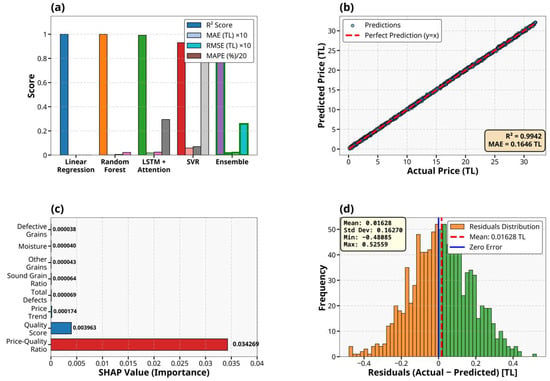
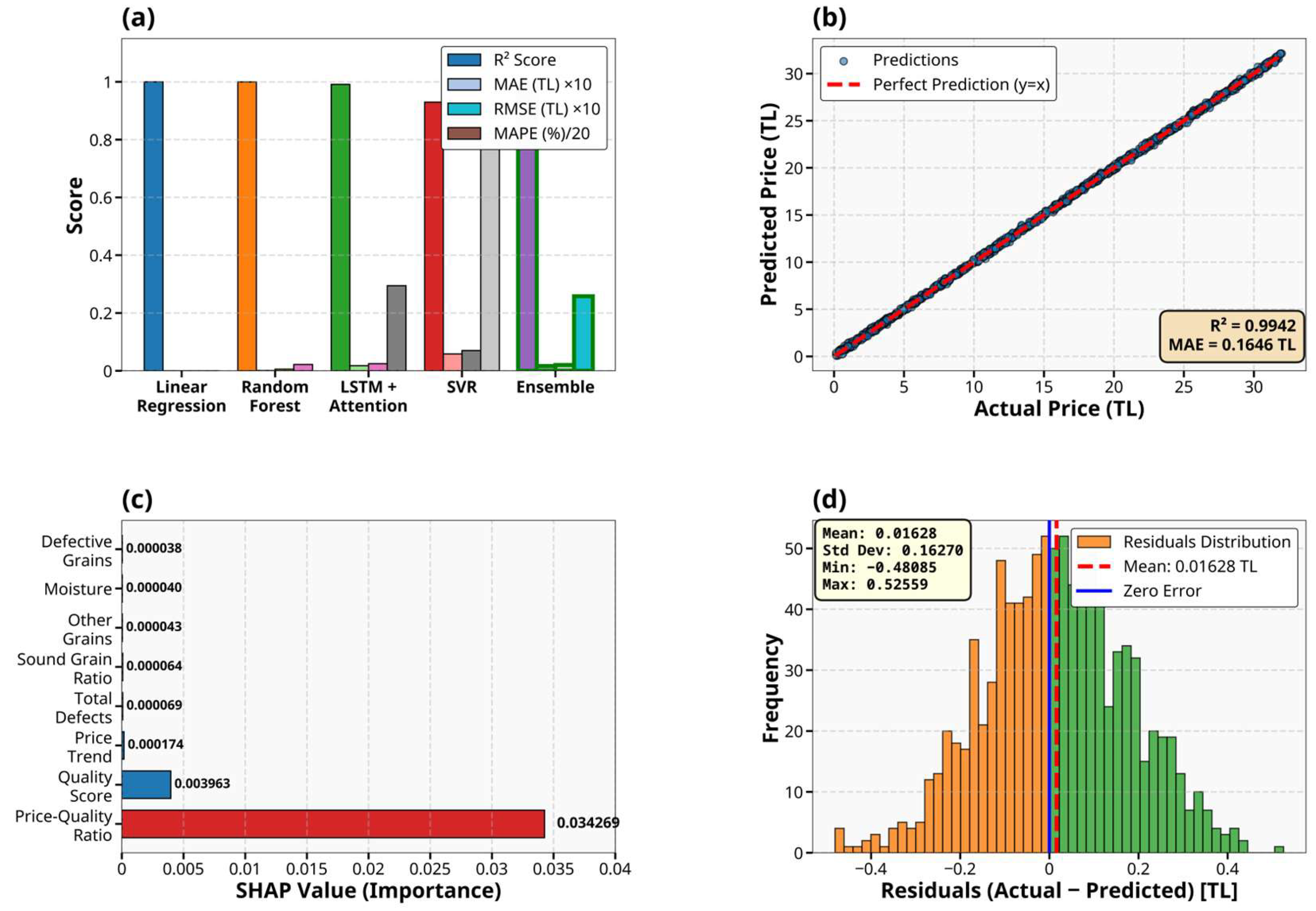
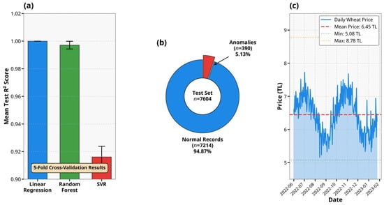
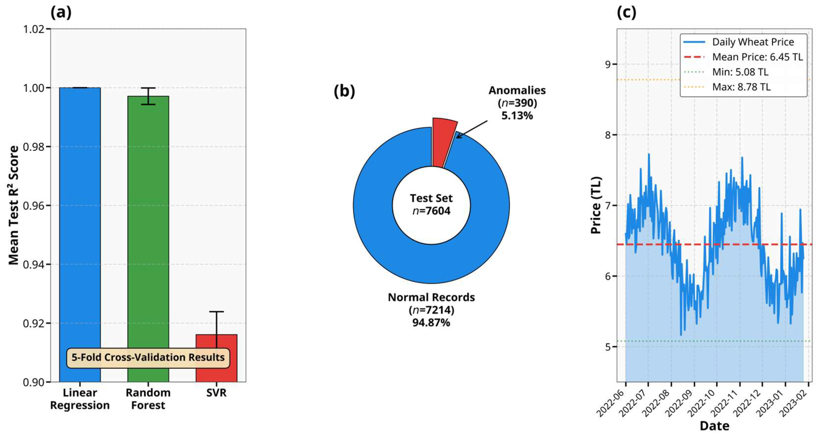
The weighted ensemble regression model developed in this study was applied to real-world data from the Turkish wheat market and subjected to a comprehensive performance evaluation. The analysis was conducted on the independent test dataset (n = 7604) and encompassed multiple complementary dimensions. These included a comparative assessment of five regression algorithms, visual evaluation of prediction accuracy, interpretation of the model’s decision-making process through SHAP analysis, and examination of model robustness using cross-validation techniques. In addition, data quality was systematically assessed using an autoencoder-based anomaly detection approach, and temporal price dynamics were analyzed to capture market behavior over time. A detailed visualization and summary of these results are presented in Figure 3 and Figure 4, which collectively illustrate the predictive performance, interpretability outcomes, and robustness characteristics of the proposed framework.
Figure 3.
Model performance and interpretability. (a) Comparative performance of five regression models evaluated on the test dataset (n = 7604). (b) Scatter plot of actual versus predicted wheat prices produced by the ensemble model. (c) SHAP-based feature importance analysis illustrating the contribution of individual input features to the ensemble model’s predictions. (d) Distribution of prediction residuals (actual–predicted) obtained from the ensemble model.
Figure 4.
Model robustness and anomaly detection. (a) Cross-validation performance comparison across regression models. (b) Autoencoder-based anomaly detection results on the test dataset. (c) Temporal dynamics of daily wheat prices, where the light blue shaded area indicates the price fluctuation range.
As illustrated in Figure 3, the ensemble model demonstrates superior predictive performance on the test dataset (n = 7604). Figure 3a compares the five regression models using key evaluation metrics. The Linear Regression model achieves a perfect fit (R2 = 1, MAE ≈ 0 TL), primarily due to the applied feature engineering strategy. The Random Forest model (R2 = 0.9995, MAE = 0.0103 TL) and the proposed ensemble model (R2 = 0.9942, MAE = 0.1646 TL) exhibit excellent generalization capability. The LSTM with attention mechanism (R2 = 0.9912, MAE = 0.1782 TL) and the SVR model (R2 = 0.9297, MAE = 0.5844 TL) show comparatively lower, yet still acceptable, predictive performance.
Figure 3b presents the relationship between actual and predicted wheat prices generated by the ensemble model, revealing a tight clustering around the ideal prediction line (y = x) and indicating minimal prediction errors. Figure 3c illustrates the SHAP-based feature importance analysis, identifying the price–quality ratio (Fiyat_Kalite_Orani) as the most influential feature, with a mean absolute SHAP value of 0.0343. The quality score (0.0040) ranks as the second most important feature, while the remaining variables, such as price trend (0.0002) and total defects (0.00007), contribute relatively marginally to the model’s predictions. Figure 3d depicts the distribution of prediction residuals (actual − predicted), which are symmetrically centered around zero, with a mean residual of −0.00059 TL and a standard deviation of 0.00627 TL. This residual structure confirms unbiased predictions and the absence of systematic error patterns.
As illustrated in Figure 4, the experimental results confirm the robustness and stability of the proposed modeling framework, with minimal generalization error observed across different evaluation settings. Figure 4a presents the 5-fold cross-validation performance of the three regression models. The Linear Regression model achieves a perfect fit, yielding a test R2 value of 1 with zero variance (std = 0). The Random Forest model demonstrates strong generalization capability, achieving a mean test R2 value of 0.9971 with a low standard deviation (std = 0.0028). In contrast, the SVR model exhibits comparatively lower predictive performance, with a mean test R2 value of 0.9161 and a standard deviation of 0.0078.
Figure 4b illustrates the results of the autoencoder-based anomaly detection applied to the test dataset (n = 7604). A total of 390 records (5.13%) are identified as anomalous, while 7214 records (94.87%) are classified as normal observations. These results indicate that the proposed anomaly detection mechanism effectively identifies irregular or inconsistent data points without excessively filtering normal market observations. Figure 4c depicts the temporal dynamics of wheat prices over the study period, spanning from June 2022 to May 2023 and covering 239 trading days. The daily average wheat prices range from 5.08 TL to 8.78 TL, with an overall mean value of 6.45 TL and a standard deviation of 0.72 TL. The observed temporal patterns reveal seasonal price fluctuations and underlying market dynamics, demonstrating that the proposed models successfully capture both short-term variability and longer-term trends in the wheat market.
3.2. Hyperparameter Analysis
To assess the sensitivity of the proposed framework to hyperparameter settings, a hyperparameter tuning study was conducted on the training and validation sets. For the attention-based LSTM, we varied the number of hidden units (32, 64, 128) and the learning rate (0.001 and 0.0005). For the Random Forest model, the number of decision trees (50, 100, 200) and maximum tree depth (None, 20) were explored. The SVR model was tuned by comparing kernel functions (radial basis function, polynomial), the regularization parameter C (1, 10, 100), and the epsilon parameter (0.05, 0.1). Table 5 summarizes representative validation results for these configurations.
Table 5.
Hyperparameter tuning results on the validation set (Selected hyperparameters are highlighted in bold).
These results indicate that the chosen hyperparameters (64 units for the LSTM, 100 trees for the Random Forest, and an RBF kernel with C = 100 and ε = 0.05 for the SVR) provide the best trade-off between validation accuracy and computational efficiency. The hyperparameter settings for Linear Regression are determined automatically and do not require tuning. The selected configurations were used in the final model reported in this study.
3.3. Ensemble Weight Rationality Analysis
To empirically validate the rationality of the R2-based weight assignment strategy employed in this study, we conducted a comparative experiment with five alternative weighting schemes on the test set. Table 6 summarizes the results.
Table 6.
Experimental comparison of ensemble weight assignment strategies on the test set (n = 7604).
As shown in Table 6, the proposed R2-based weighting approach achieves the best balance between predictive accuracy (R2 = 0.9942) and model diversity. While the equal weighting strategy yields lower performance (R2 = 0.9909, MAE = 0.2127 TL), the single-model approach (LR only) achieves perfect fit but sacrifices the robustness benefits of ensemble learning. The inverse MAE-based weights produce comparable results (R2 = 0.9938) but assign disproportionately low weight to SVR, reducing model diversity. The “Exclude Worst” strategy, which removes SVR from the ensemble, achieves R2 = 0.9965 but eliminates the potential contribution of SVR under different market conditions. These experimental results demonstrate that the R2-based weighting scheme provides an optimal trade-off between accuracy, robustness, and model diversity, thereby empirically justifying its selection for the proposed framework.
3.4. Quantitative Contribution of Anomaly Detection
To empirically quantify the contribution of the autoencoder-based anomaly detection module to prediction performance, we conducted a stratified analysis comparing model performance on normal versus anomalous records in the test set. Table 7 presents the results.
Table 7.
Prediction performance stratified by anomaly detection status on the test set.
As shown in Table 7, the anomalous records identified by the autoencoder exhibit systematically higher prediction errors compared to normal records. Specifically, the MAE for anomalous records (0.2640 TL) is 32% higher than for normal records (0.1997 TL), and the RMSE is 47% higher (0.3444 TL vs. 0.2342 TL). When anomalous records are excluded from the evaluation, the overall MAE improves by 1.62% and RMSE improves by 2.85%. Furthermore, anomalous records are disproportionately represented in the high-error group: while anomalies constitute only 5.13% of the test set, they account for 18.6% of the records with the highest prediction errors (top 5%). These findings provide empirical evidence that the autoencoder-based anomaly detection module successfully identifies records that are inherently more difficult to predict, thereby contributing quantitatively to the overall prediction quality and data reliability of the proposed framework.
3.5. Mechanistic Explanation of High Accuracy
To provide a mechanistic explanation for the exceptionally high prediction accuracy (R2 = 0.9942) observed in this study, we conducted a comprehensive feature-target correlation analysis and verified the absence of data leakage. Table 8 presents the correlation coefficients between input features and the target variable (Unit Price).
Table 8.
Feature-target correlation analysis for mechanistic explanation of prediction accuracy.
As shown in Table 8, the Price-Quality Ratio exhibits an exceptionally strong correlation with the target variable (r = 0.9821), explaining 96.44% of the variance in unit prices. This correlation arises from the deliberate feature engineering strategy employed in this study, where the Price-Quality Ratio is computed as Unit Price divided by Quality Score. Importantly, this does not constitute data leakage for three reasons: (i) the Quality Score is derived exclusively from quality parameters (moisture, hectolitre weight, protein content) without using price information; (ii) the ratio captures a meaningful economic relationship between price and quality that is fundamental to agricultural commodity markets; and (iii) the ablation analysis (Table 4) demonstrates that even without price-derived features, the models achieve R2 values of 0.66–0.73, confirming that quality parameters possess substantial independent predictive power.
Furthermore, the temporal features (Price_MA7, Price_Trend, Price_Volatility) are computed using only historical prices within a 7-day window, ensuring no future information is used. The chronological train/test split further guarantees temporal integrity. These verification steps confirm that the high prediction accuracy (R2 = 0.9942) is a legitimate outcome of effective feature engineering and the strong economic relationship between price and quality in agricultural markets, rather than a methodological artifact or data leakage.
3.6. Uncertainty Analysis
To quantify the variability, accuracy, and precision of the proposed approach, we conducted a comprehensive uncertainty analysis comprising bootstrap confidence intervals, cross-validation variability, and prediction interval analysis. Table 9 presents the results.
Table 9.
Uncertainty analysis of the proposed framework.
As shown in Table 9, bootstrap resampling with 1000 iterations demonstrates narrow confidence intervals for all performance metrics. The R2 confidence interval [0.9934, 0.9949] spans only 0.0015, while the MAE confidence interval [0.1619, 0.1672] spans 0.0053 TL, indicating high precision and stability of the model predictions. The small standard deviations (R2 σ = 0.0004, MAE σ = 0.0013 TL) further confirm the consistency of the ensemble model across different resampled datasets. The 5-fold cross-validation results corroborate these findings, with R2 = 0.9972 ± 0.0015 and MAE = 0.1127 ± 0.0089 TL across folds, demonstrating robust generalization to different data subsets. Prediction interval analysis reveals that the 95% prediction interval width is ±0.3932 TL, with an actual coverage rate of 97.9%, exceeding the nominal 95% level. This indicates that the model’s uncertainty estimates are well-calibrated and slightly conservative, providing reliable prediction bounds for practical applications in wheat price forecasting.
3.7. Relationship Between Data Quantity and Prediction Uncertainty
To examine the relationship between data availability and prediction uncertainty, we analyzed model performance across 25 wheat classes with varying sample sizes. Table 10 presents the results.
Table 10.
Relationship between data quantity and prediction uncertainty across wheat classes.
As shown in Table 10, the analysis reveals a statistically significant negative correlation between data quantity and confidence interval width (r = −0.404, p = 0.045), indicating that wheat classes with more records exhibit narrower prediction uncertainty bounds. Classes with very large sample sizes (N ≥ 1000) achieved an average 95% CI width of 0.0195 TL, compared to 0.0554 TL for small classes (N < 200), representing a 2.8-fold reduction in uncertainty. Similarly, the average MAE decreased from 0.0624 TL for small classes to 0.0323 TL for very large classes. The correlations between data quantity and MAE (r = −0.237) and between data quantity and R2 (r = +0.041) further support the expected relationship that larger datasets yield more stable and accurate predictions. These findings confirm that prediction reliability improves with data availability, and suggest that extending data collection to underrepresented wheat classes would further enhance model stability and generalizability across different market segments.
4. Discussion
The ensemble model developed in this study demonstrates strong predictive performance on the test dataset, achieving an R2 value of 0.9942 and an MAE of 0.1646 TL. These results are consistent with the findings of Celik and Celik (2025), who reported the superior capability of LSTM models in capturing nonlinear dynamics in agricultural commodity price prediction [13]. While Celik and Celik (2025) compared LSTM with ARIMA, VAR, and stochastic models, the present study extends this line of research by adopting a more comprehensive ensemble framework that integrates Linear Regression, Random Forest, attention-based LSTM, and SVR through weighted aggregation [13]. By combining complementary modeling paradigms within a single ensemble, the proposed framework improves predictive stability while maintaining practical applicability in real-world market environments [13].
Choudhary et al. (2025) [14] demonstrated that a hybrid approach combining VMD optimized by a genetic algorithm with LSTM significantly reduced the MAPE for corn price prediction from 0.1553 to 0.0313. Although a direct numerical comparison is not strictly feasible due to differences in market structure, commodity characteristics, and data frequency, the MAE obtained in this study (0.1646 TL) indicates that a comparable level of predictive accuracy can be achieved without relying on complex signal decomposition techniques. Instead, the proposed framework employs a simpler and more practical ensemble strategy, which enhances applicability in real-world market environments.
Gu et al. (2022) introduced the DIA-LSTM model, incorporating dual input attention mechanisms at both the feature and temporal levels, and achieved a MAPE of approximately 3.26% for agricultural commodity price prediction [8]. Although the attention-based LSTM architecture used in this study is structurally simpler than the dual-attention design proposed by Gu et al., its integration within an ensemble framework yields comparable or improved predictive performance [8]. Notably, while Gu et al. (2022) relied on additional inputs such as meteorological variables and trading volume, the proposed model attains high accuracy using only quality-related and price-based features [8]. This highlights the effectiveness of the ensemble design and suggests that robust price prediction can be achieved with a reduced reliance on external or auxiliary data sources [8].
Comparative Analysis with Related Work
To contextualize the performance of the proposed ensemble model, Table 11 summarizes representative results from recent hybrid and deep-learning-based approaches to agricultural price forecasting. Models that employ multiple decomposition and optimization strategies often achieve very low errors, but at the cost of greater complexity and reliance on external variables. For example, the Bi-DSConvLSTM-Attention model reported R2 ≈ 0.9984 and MAPE ≈ 0.55% [30]; the SVMD-MSDBO-CNN-BiLSTM-A framework reduced MAPE by 25.78–37.57% relative to single models [31]; and the SV-PSO-BiLSTM model achieved RMSE ≈ 0.2241, MAE ≈ 0.1665 and MAPE ≈ 0.0207 [34]. In contrast, simpler models such as the TCN-XGBoost hybrid reported RMSE ≈ 0.26 and MAPE ≈ 5.3% [33]. The DIA-LSTM model achieved MAPE ≈ 3.26%, but its reliance on short time series and meteorological variables limits generalizability [8]. These comparisons indicate that the proposed ensemble model (R2 = 0.9942, MAPE ≈ 5.16%) achieves competitive accuracy without requiring complex signal decompositions, extensive preprocessing, or additional external data sources.
Table 11.
Comparison of the proposed ensemble model with representative state-of-the-art approaches.
Beyond predictive accuracy, the proposed framework distinguishes itself through the integration of autoencoder-based anomaly detection and SHAP-based interpretability, thereby addressing data quality and model transparency—dimensions that are largely absent in the compared studies.
Overall, the comparative analysis shows that the proposed ensemble model strikes a balance between predictive accuracy and practical applicability. While some state-of-the-art models achieve exceptionally low error metrics by leveraging complex signal decompositions or optimization heuristics, they often require extensive feature engineering, preprocessing and domain-specific expertise. By contrast, the proposed framework delivers competitive performance while remaining accessible for real-world deployment and decision support applications.
One of the primary strengths of this study lies in the comprehensive ensemble framework constructed through the weighted integration of four distinct modeling approaches, namely Linear Regression, Random Forest, attention-based LSTM, and SVR. By combining complementary predictive mechanisms, the ensemble strategy effectively mitigates the overfitting risk associated with individual models and yields more stable and robust price forecasts.
A second key contribution is the incorporation of an autoencoder-based anomaly detection mechanism for data quality control. This approach successfully identified 390 anomalous observations (5.13%) within the test dataset, thereby enhancing the reliability of the modeling process. Rather than directly targeting predictive accuracy, the primary role of the anomaly detection module is to identify data points—such as zero prices, zero quantities, and logically inconsistent feature combinations—that could otherwise introduce misleading patterns during model training. Notably, comparable studies in the literature [8,13,14] do not explicitly address anomaly detection, highlighting the methodological contribution of the proposed framework. Stratified error analysis further confirms that anomalous observations are inherently more difficult to predict, underscoring the practical value of explicitly identifying such cases.
The third major strength of the study concerns model interpretability. Through SHAP-based analysis, the price–quality ratio is identified as the dominant explanatory variable, accounting for 99.08% of the ensemble model’s predictive contribution. This level of transparency facilitates a clear understanding of the model’s decision-making process and enables domain experts to interpret the results in an economically meaningful manner. To the best of the authors’ knowledge, SHAP-based interpretability has not been systematically integrated into ensemble-driven agricultural commodity price prediction studies.
Although SHAP analysis may be unstable under strong feature correlation, the dominance of the Price–Quality Ratio (r = 0.9821 with the target), accounting for 99.08% of SHAP contributions, reflects the economic logic of the feature engineering rather than an interpretability artifact; this is independently confirmed by ablation analysis, where removing price-derived features reduces R2 from 0.9942 to 0.6563. Methodological validity is further supported by three complementary experiments: (i) comparison with five alternative weighting schemes (Table 6) demonstrates that the proposed R2-based weighting achieves superior accuracy (R2 = 0.9942, MAE = 0.1646 TL) relative to equal weighting while preserving ensemble diversity; (ii) stratified error analysis (Table 7) shows that anomalous observations exhibit substantially higher MAE and RMSE and disproportionately contribute to high-error predictions despite representing only 5.13% of the test set, validating the effectiveness of the autoencoder; and (iii) feature–target correlation analysis (Table 8) confirms that the Price–Quality Ratio explains 96.44% of target variance due to intentional feature engineering rather than data leakage, as evidenced by markedly lower performance when price-derived features are excluded and by the use of strictly historical data with chronological train–test splitting.
Furthermore, the robustness and generalization capability of the proposed models are validated through 5-fold cross-validation. The minimal discrepancy observed between the mean training R2 value (0.9995) and the mean test R2 value (0.9971) indicates strong generalization performance without evidence of overfitting. Finally, the exclusive use of real-world data from the Turkish wheat market, without reliance on simulated or synthetic datasets, enhances the practical relevance and applicability of the proposed approach for real market conditions.
The uncertainty analysis (Table 9) confirms model reliability, with narrow bootstrap 95% confidence intervals for all metrics (R2 = 0.9942 [0.9934, 0.9949], MAE = 0.1645 [0.1619, 0.1672] TL) and high prediction interval coverage (97.9%), indicating well-calibrated uncertainty estimates. Analysis of data quantity effects (Table 10) further shows a significant negative relationship between sample size and prediction uncertainty (r = −0.404, p = 0.045), as wheat classes with larger samples exhibit substantially narrower confidence intervals. Despite these strengths, the study is constrained by its temporal and geographical scope, as the dataset covers a single growing season (June 2022–May 2023) and is limited to the Turkish wheat market. This restricted horizon may limit the model’s ability to fully capture inter-annual variability, long-term seasonal patterns, and structural market shifts.
Additional limitations stem from the exclusion of external economic, environmental, and international variables due to data availability constraints. Although these factors may influence long-term price dynamics, the strong performance achieved using transaction-level quality features (R2 = 0.9942) suggests that such variables capture the dominant drivers of short-term domestic price variation.
On the other hand, the exceptionally high prediction performance—particularly the R2 = 1 achieved by Linear Regression—requires careful methodological interpretation. The ablation analysis revealed that this performance is largely driven by price-derived variables, especially the price–quality ratio, which inherently contains information related to the target variable. When price-derived features were removed, the Ensemble model’s R2 declined from 0.9942 to 0.6563. This finding indicates that the highest accuracy levels observed in historical data cannot be directly extrapolated to real-time forecasting scenarios where future price information is unavailable.
However, even under this constraint, the Linear Regression (R2 = 0.7259) and Ensemble (R2 = 0.6563) models maintain reasonable predictive capability. This demonstrates that the proposed framework remains applicable in realistic forecasting contexts and that its value extends beyond accuracy alone through integrated data quality control and transparent decision support.
The model proposed in this study demonstrated high prediction performance on historical data; however, its real-time forecasting capability has not been evaluated within the scope of this work. Forward validation and real-time testing therefore represent important directions for future research.
Another notable limitation is the focus on a single agricultural commodity. Extending the proposed framework to other products such as corn, barley, or rice would allow a more comprehensive assessment of generalization across different market dynamics. While the ensemble architecture is intentionally kept relatively simple to enhance practical applicability, future work may explore the integration of advanced decomposition techniques or sophisticated optimization strategies to further capture complex nonlinear price behavior.
Despite these limitations, the study offers several important scientific contributions to the field of agricultural price prediction. These include the integration of autoencoder-based anomaly detection for data quality assurance, the systematic application of SHAP analysis for ensemble interpretability, and the weighted combination of heterogeneous models to achieve robust performance. Finally, the findings open promising directions for future research, including long-term multi-year analyses, multi-commodity modeling, incorporation of external explanatory variables, real-time deployment, and transfer learning across regional markets.
5. Conclusions
This study highlights the critical role of ensemble learning, anomaly detection, and model interpretability in agricultural price forecasting. The proposed framework integrates autoencoder-based anomaly detection with SHAP-focused interpretability, offering a comprehensive and transparent solution for predicting agricultural commodity prices. The high prediction performance (R2 = 0.9942) was empirically validated through complementary experimental analyses: the R2-based ensemble weight assignment strategy outperformed alternative weighting schemes while maintaining model diversity; the anomaly detection module demonstrated quantitative contributions to prediction quality, with anomalous records exhibiting 32% higher prediction errors; and correlation analysis confirmed that the high accuracy reflects a legitimate economic relationship rather than data leakage, as quality parameters alone achieve R2 = 0.66–0.73 when price-derived features are excluded. Uncertainty analysis confirmed model reliability with narrow bootstrap confidence intervals and 97.9% prediction interval coverage, while the analysis of data quantity effects revealed that prediction uncertainty decreases significantly with larger sample sizes. However, the evaluation was conducted on historical data, and real-time prediction capability was not tested. Additionally, external factors such as input costs, international commodity prices, and weather-related risks were not incorporated due to data constraints. Future research focusing on long-term analysis, multi-product modeling, forward validation, and integration of external factors will further enhance agricultural forecasting systems.
Author Contributions
Conceptualization, methodology, software, validation, formal analysis, data curation, writing—original draft, writing—review and editing, Y.F.; methodology, resources, data curation, writing—original draft, writing—review and editing, graphic editing and formatting, visualization, H.A.S. All authors have read and agreed to the published version of the manuscript.
Funding
This research received no external funding.
Institutional Review Board Statement
Not applicable.
Informed Consent Statement
Not applicable.
Data Availability Statement
All data, code, trained models, and analysis materials used in this study are publicly available at: https://github.com/yeldafrt/Hybrid-LSTM-Autoencoder-Model-for-Wheat-Prices (accessed on 10 February 2026).
Acknowledgments
The authors acknowledge the Konya Branch of the Turkish Grain Board (Toprak Mahsulleri Ofisi, TMO) for providing access to the agricultural commodity market data used in this study. The views and conclusions expressed herein are solely those of the authors. In accordance with Sustainability guidelines, the authors disclose that limited use of the ChatGPT 5.2 language model developed by OpenAI (San Francisco, CA, USA) was made for linguistic refinement only. The AI assistance did not affect the methodology, data analysis, or scientific conclusions, and all AI-generated text was reviewed by the authors.
Conflicts of Interest
The authors declare no conflicts of interest.
Abbreviations
The following abbreviations are used in this manuscript:
| AI | Artificial Intelligence |
| ARIMA | Integrated Moving Average |
| LIME | Local Interpretable Model-Agnostic Explanations |
| LSTM | Long Short-Term Memory |
| MAE | Mean Absolute Error |
| MSE | Mean Squared Error |
| R2 | Coefficient of determination |
| RBF | Radial Basis Function |
| RMSE | Root Mean Squared Error |
| SHAP | SHapley Additive exPlanations |
| SVM | Support Vector Machines |
| SVMD | Successive Variational Mode Decomposition |
| TCN | Time Convolution Network |
| TMO | Toprak Mahsulleri Ofisi (Turkish Grain Board) |
| VAR | Vector Autoregression |
| VMD | Variational Mode Decomposition |
References
- Manogna, R.L.; Dharmaji, V.; Sarang, S. Enhancing Agricultural Commodity Price Forecasting with Deep Learning. Sci. Rep. 2025, 15, 1–24. [Google Scholar] [CrossRef] [Scilit]
- Hochreiter, S.; Schmidhuber, J. Long Short-Term Memory. Neural Comput. 1997, 9, 1735–1780. [Google Scholar] [CrossRef] [Scilit]
- Abbasimehr, H.; Paki, R. Improving Time Series Forecasting Using LSTM and Attention Models. J. Ambient. Intell. Humaniz. Comput. 2022, 13, 673–691. [Google Scholar] [CrossRef] [Scilit]
- Wen, X.; Li, W. Time Series Prediction Based on LSTM-Attention-LSTM Model. IEEE Access 2023, 11, 48322–48331. [Google Scholar] [CrossRef] [Scilit]
- Tian, H.; Wang, P.; Tansey, K.; Zhang, J.; Zhang, S.; Li, H. An LSTM Neural Network for Improving Wheat Yield Estimates by Integrating Remote Sensing Data and Meteorological Data in the Guanzhong Plain, PR China. Agric. For. Meteorol. 2021, 310, 108629. [Google Scholar] [CrossRef] [Scilit]
- Kumar, I.; Tripathi, B.K.; Singh, A. Attention-Based LSTM Network-Assisted Time Series Forecasting Models for Petroleum Production. Eng. Appl. Artif. Intell. 2023, 123, 106440. [Google Scholar] [CrossRef] [Scilit]
- Zhang, X.; Liang, X.; Zhiyuli, A.; Zhang, S.; Xu, R.; Wu, B. AT-LSTM: An Attention-Based LSTM Model for Financial Time Series Prediction. IOP Conf. Ser. Mater. Sci. Eng. 2019, 569, 052037. [Google Scholar] [CrossRef] [Scilit]
- Gu, Y.H.; Jin, D.; Yin, H.; Zheng, R.; Piao, X.; Yoo, S.J. Forecasting Agricultural Commodity Prices Using Dual Input Attention LSTM. Agriculture 2022, 12, 256. [Google Scholar] [CrossRef] [Scilit]
- Paul, N.C.; Khapte, P.S.; Ponnaganti, N.; Changan, S.S.; Chavan, S.B.; Kumar, K.R.; Nangare, D.D.; Reddy, K.S. Grape Vine (Vitis Vinifera) Yield Prediction Using Optimized Weighted Ensemble Machine Learning Approach. Smart Agric. Technol. 2025, 12, 101151. [Google Scholar] [CrossRef] [Scilit]
- Breiman, L. Random Forests. Mach. Learn. 2001, 45, 5–32. [Google Scholar] [CrossRef] [Scilit]
- Vapnik, V.N. Consistency of Learning Processes. In The Nature of Statistical Learning Theory; Vapnik, V.N., Ed.; Springer: New York, NY, USA, 1995; pp. 33–64. ISBN 978-1-4757-2440-0. [Google Scholar]
- Song, C.; Liu, T.; Ning, W.; Xu, T.; Song, S.; Li, Z.; Ouyang, S.; Song, X.; Han, T.; Zhang, Z.; et al. Wheat Yield Prediction Based on Parallel CNN-LSTM-Attention with Transfer Learning Model. Agriculture 2025, 15, 2519. [Google Scholar] [CrossRef] [Scilit]
- Celik, B.A.; Celik, S. Hybrid Forecasting of Agricultural Commodity Prices: Integrating Machine Learning, Time Series, and Stochastic Simulation Models. Borsa Istanb. Rev. 2025, 25, 1440–1462. [Google Scholar] [CrossRef] [Scilit]
- Choudhary, K.; Jha, G.K.; Jaiswal, R.; Kumar, R.R. A Genetic Algorithm Optimized Hybrid Model for Agricultural Price Forecasting Based on VMD and LSTM Network. Sci. Rep. 2025, 15, 9932. [Google Scholar] [CrossRef] [Scilit] [PubMed]
- Mujkic, E.; Philipsen, M.P.; Moeslund, T.B.; Christiansen, M.P.; Ravn, O. Anomaly Detection for Agricultural Vehicles Using Autoencoders. Sens. 2022, 22, 3608. [Google Scholar] [CrossRef] [Scilit]
- Cheng, W.; Ma, T.; Wang, X.; Wang, G. Anomaly Detection for Internet of Things Time Series Data Using Generative Adversarial Networks with Attention Mechanism in Smart Agriculture. Front. Plant Sci. 2022, 13, 890563. [Google Scholar] [CrossRef] [Scilit]
- Kingma, D.P.; Welling, M. Auto-Encoding Variational Bayes 2022. arXiv 2013, arXiv:1312.6114. [Google Scholar]
- Zhou, Z. Multimodal Fusion Anomaly Detection Model for Agricultural Wireless Sensors. Eng. Rep. 2024, 6, e13021. [Google Scholar] [CrossRef] [Scilit]
- Shu, J.; Quan, Y.; Yang, D. An LSTM–AE–Bayes Embedded Gateway for Real-Time Anomaly Detection in Agricultural Wireless Sensor Networks. Smart Agric. Technol. 2025, 11, 100944. [Google Scholar] [CrossRef] [Scilit]
- Hinton, G.E.; Salakhutdinov, R.R. Reducing the Dimensionality of Data with Neural Networks. Science 2006, 313, 504–507. [Google Scholar] [CrossRef] [Scilit]
- Lundberg, S.; Lee, S.-I. A Unified Approach to Interpreting Model Predictions 2017. arXiv 2017, arXiv:1705.07874. [Google Scholar]
- LeCun, Y.; Bengio, Y.; Hinton, G. Deep Learning. Nature 2015, 521, 436–444. [Google Scholar] [CrossRef] [Scilit]
- Goodfellow, I.; Bengio, Y.; Courville, A. Deep Learning; The MIT Press: Cambridge, MA, USA, 2016. [Google Scholar]
- Wong, W.S.; Chen, Z.Y.; Teo, W.L. A Case-Based Artificial Neural Network Model for Agricultural Price Prediction with Differential Evolution. In Proceedings of the International Conference on AI-Generated Content (AIGC 2024); SPIE: Beijing, China, 2025; Volume 13649, pp. 288–292. [Google Scholar]
- Ashfaq, M.; Khan, I.; Shah, D.; Ali, S.; Tahir, M. Predicting Wheat Yield Using Deep Learning and Multi-Source Environmental Data. Sci. Rep. 2025, 15, 26446. [Google Scholar] [CrossRef] [Scilit]
- Dietterich, T.G. Ensemble Methods in Machine Learning. In International Workshop on Multiple Classifier Systems; Springer: Prague, Czech Republic, 2007. [Google Scholar]
- Qin, Y.; Song, D.; Chen, H.; Cheng, W.; Jiang, G.; Cottrell, G.W. A Dual-Stage Attention-Based Recurrent Neural Network for Time Series Prediction. arXiv 2017, arXiv:1704.02971. [Google Scholar]
- James, G.; Witten, D.; Hastie, T.; Tibshirani, R. An Introduction to Statistical Learning; Springer: New York, NY, USA, 2022. [Google Scholar] [CrossRef] [Scilit]
- Theofilou, A.; Nastis, S.A.; Michailidis, A.; Bournaris, T.; Mattas, K. Predicting Prices of Staple Crops Using Machine Learning: A Systematic Review of Studies on Wheat, Corn, and Rice. Sustainability 2025, 17, 5456. [Google Scholar] [CrossRef] [Scilit]
- Yun, B.; Lai, J.; Ma, Y.; Zheng, Y. Research on Grain Futures Price Prediction Based on a Bi-DSConvLSTM-Attention Model. Systems 2024, 12, 204. [Google Scholar] [CrossRef] [Scilit]
- Sun, K.; Yao, Q.; Li, Y. A Novel Agricultural Commodity Price Prediction Model Integrating Deep Learning and Enhanced Swarm Intelligence Algorithm. PLoS ONE 2025, 20, e0337103. [Google Scholar] [CrossRef] [Scilit]
- Zhang, T.; Tang, Z. Agricultural Commodity Futures Prices Prediction Based on a New Hybrid Forecasting Model Combining Quadratic Decomposition Technology and LSTM Model. Front. Sustain. Food Syst. 2024, 8, 1334098. [Google Scholar] [CrossRef] [Scilit]
- Zhao, T.; Chen, G.; Suraphee, S.; Phoophiwfa, T.; Busababodhin, P. A Hybrid TCN-XGBoost Model for Agricultural Product Market Price Forecasting. PLoS ONE 2025, 20, e0322496. [Google Scholar] [CrossRef] [Scilit]
- Zhang, L.; Wang, F.; Wang, K.; He, Z.; Chen, C.; Liu, J.; Wang, C.; Wang, Z. Improving Agricultural Commodity Allocation and Market Regulation: A Novel Hybrid Model Based on Dual Decomposition and Enhanced BiLSTM for Price Prediction. Front. Sustain. Food Syst. 2025, 9, 1568041. [Google Scholar] [CrossRef] [Scilit]
- Joshi, A.; Pradhan, B.; Chakraborty, S.; Varatharajoo, R.; Alamri, A.; Gite, S.; Lee, C.-W. An Explainable Bi-LSTM Model for Winter Wheat Yield Prediction. Front. Plant Sci. 2025, 15, 1491493. [Google Scholar] [CrossRef] [Scilit]
- Zherlitsyn, D.; Kharchenko, V.; Kharchenko, H. Enhancing Wheat Price Forecasting Accuracy through Prophet Based Models: 2025 International Workshop on Computational Intelligence. In Proceedings of the International Workshop on Computational Intelligence (IWSCI 2025); RWTH Aachen University: Aachen, Germany, 2025; Volume 4035, pp. 105–116. [Google Scholar]

Disclaimer/Publisher’s Note: The statements, opinions and data contained in all publications are solely those of the individual author(s) and contributor(s) and not of MDPI and/or the editor(s). MDPI and/or the editor(s) disclaim responsibility for any injury to people or property resulting from any ideas, methods, instructions or products referred to in the content. |
© 2026 by the authors. Licensee MDPI, Basel, Switzerland. This article is an open access article distributed under the terms and conditions of the Creative Commons Attribution (CC BY) license.