Article

Water Scarcity Risk Assessment for Multi-Administrative Units in Agricultural Watersheds Using Integrated QSWAT–WEAP and GIS-Based Approach


by
Jirawat Supakosol
1,
Haris Prasanchum
2,*,
Anongrit Kangrang
3,
Rattana Hormwichian
3,
Piyapatr Busababodhin
4,
Krit Sriworamas
5,
Somphinith Muangthong
6,
Kewaree Pholkern
7,
Sarayut Wongsasri
8 and
Winai Chaowiwat
9
1
Faculty of Industry and Technology, Rajamangala University of Technology Isan, Sakon Nakhon Campus, Sakon Nakhon 47160, Thailand
2
Faculty of Engineering, Rajamangala University of Technology Isan, Khon Kaen Campus, Khon Kaen 40000, Thailand
3
Faculty of Engineering, Maha Sarakham University, Maha Sarakham 44150, Thailand
4
Faculty of Science, Maha Sarakham University, Maha Sarakham 44150, Thailand
5
Faculty of Engineering, Ubon Ratchathani University, Ubon Ratchathani 34190, Thailand
6
Faculty of Engineering and Technology, Rajamangala University of Technology Isan, Nakhon Ratchasima 30000, Thailand
7
Faculty of Agriculture, Khon Kaen University, Khon Kaen 40002, Thailand
8
Center for Water Resources Engineering and Environment, Faculty of Engineering, Khon Kaen University, Khon Kaen 40002, Thailand
9
Hydro-Informatics Innovation Division, Hydro Informatics Institute, Bangkok 10400, Thailand
*
Author to whom correspondence should be addressed.
Sustainability 2026, 18(4), 1932; https://doi.org/10.3390/su18041932
Submission received: 8 January 2026 / Revised: 6 February 2026 / Accepted: 10 February 2026 / Published: 13 February 2026

Abstract

Water shortage is a critical problem that affects the sustainability of the agricultural sector in Northeastern Thailand, especially areas located far from major rivers. This study developed an integrated QSWAT–WEAP modeling system combined with GIS-based spatial analysis for water shortage risk assessment at the sub-district level in Maha Sarakham Province, covering 5292 sq.km and 133 sub-districts. The system bridges the institutional gap between hydrological sub-watershed boundaries and administrative jurisdictions, enabling model outputs that directly support local governance decision-making. The QSWAT model simulated sub-watershed streamflow while the WEAP model evaluated water balance against water demand from five sectors. QSWAT validation (2017–2023) achieved R2 = 0.72, NSE = 0.70, and RSR = 0.54, while WEAP verification yielded R2 of 0.66–0.80 and NSE of 0.65–0.71. In the spatial analysis, 106 of 133 sub-districts (79.7%) experienced low water availability. Agriculture was the dominant sector in terms of water demand, which has increased at an average rate of 1.7% annually and accounted for 88.7% of total demand in the study period. According to the temporal analysis, the dry season was the most critical period, with peak water shortage of 99.2% in March. Overall, 105 of 133 sub-districts (78.9%) were classified as having water shortages of moderate to very high severity. These findings provide a quantitative basis for sustainable water resource management planning and drought mitigation, thus helping to enhance agricultural sustainability in Maha Sarakham Province.

1. Introduction

Climate change has significantly affected hydrologic cycles and water resource management over the past decade. In particular, the increasing global average temperature is leading to changes in rainfall, runoff, and evaporation rates [1], which in turn cause water-related disasters of increasing severity such as the unusual prolonged drought experienced in many regions around the world during 2020–2023 [2]. Impact assessments and plans to cope with the effects of climate change require numeric models with high precision for the simulation of hydrological processes and prediction of global changes [3,4]. Southeast Asia is one region that has been significantly affected by climate change. Cambodia, Vietnam, and Laos, in particular, were affected by drought in 2020–2022, impacting agricultural productivity and food security in the region [5]. Water management in this region is complicated, as both physical and socioeconomic factors must be considered. As a result, models for hydrologic and water management have become more desirable [6], leading to the development of decision support systems integrating models for systematic problem analysis and strategic planning regarding water management [3,7]. In this context, Thailand has experienced severe drought over the past decade; especially the northeastern region, where agricultural losses exceeded approximately USD 430 million (THB 15 billion) in 2022, representing a significant economic impact on the region’s predominantly rain-fed agricultural sector [8,9]. The application of hydrologic models for water prediction and management planning has been extensively explored in Thailand [10]. However, most previous studies have relied predominantly on single-model approaches for analyses, for example, to assess the impacts of land use changes on runoff in the Northeast [11] and analyze water demand in the Chao Phraya River Basin [12]. Despite the demonstrated potential of multi-model integration for enhancing the capacity of water resource analyses [7], studies in Thailand employing such integrated approaches remain limited, particularly at the local administrative scale [13]. The development of spatial water assessment and monitoring systems is necessary to improve the efficiency of water resource management in the country [6], especially systems supporting decision-making at the local level that are integrated with the national water management system [7,14]. Integrating hydrologic model technology with geographic information systems is essential for the future development of decision support systems for water management [15,16]. These observations underscore the need for integrated modeling frameworks that combine hydrological simulation with water resource planning at administrative scales that are relevant to local decision-making.
Spatial modeling approaches that integrate hydrologic simulations with water budget analyses have been increasingly applied worldwide for water resource assessment, as they enable geospatial and temporal visualization that supports stakeholder understanding. In Cambodia, Touch et al. [17] applied integrated hydrologic and water budget models to assess the impacts of urban development on water security in the Tonle Sap Lake Tributary Basin, while Tran et al. [16] demonstrated effective water management planning for semi-arid areas in Cuba. Similarly, Khoi et al. [18] assessed water scarcity risk at the sub-basin level in Vietnam. Among hydrologic models, SWAT is widely recognized for its capacity to simulate complex hydrologic processes at the sub-watershed level [19]. Studies have demonstrated SWAT’s effectiveness across diverse geographic contexts, including for assessing impact of land-use change on runoff in India [20], climate change effects on reservoir storage in Turkey [21], and water scarcity in drought-prone areas of Ethiopia [22]. The advancement of SWAT as a public domain model enabled its integration with QGIS through the Quantitative Soil and Water Assessment Tool (QSWAT) [23,24,25,26], enhancing capacity for spatial analysis. QSWAT has been widely applied in South Asia and Southeast Asia to assess the effects of climate change on rain-fed agricultural sites [27], analyze geospatial and temporal hydrologic elements at the regional level in Thailand [28,29,30], and evaluate water resources for dry-season crop cultivation planning [31]. Similarly, the Water Evaluation and Planning System (WEAP) has been extensively applied for water balance and water scarcity analyses in drought-prone areas across various temporal scenarios [32,33], including water allocation analysis in Iraq [34], irrigation and water scarcity assessment in Morocco [35], and risk assessment for irrigated areas in Vietnam’s Mekong Delta [36]. In Thailand and Southeast Asia, Kuntiyawichai and Wongsasri [37] assessed the impacts of drought on water security at the community level, while Forni et al. [38] and Guzman et al. [39] developed decision support systems for water management in agricultural sites characterized by water scarcity risk in Cambodia and the Philippines. Collectively, these studies demonstrate that while QSWAT and WEAP have been successfully applied individually across diverse regions, their integration for sub-district level water scarcity assessments in agricultural watersheds remains largely unexplored.
Notably, the previous studies lack small-scale spatial analyses, especially at the local government organization level [40,41]. Candido et al. [7] and Nagata et al. [42] have reported the challenges associated with developing an output system that can be easily understood by local users. Thailand has encountered several constraints in local water management, such as a lack of efficient tools for analyzing and forecasting water situations and limited data sharing between central and local government organizations, leading to inefficiency in drought management at the local level. Therefore, this research considers the integration of QSWAT and WEAP models to address these constraints through a sub-district level water scarcity risk assessment system designed to display the output in clear maps and graphs. Moreover, an open-source model was used for system modification to fit the local context. The integration of both models also increases the capacity for hydrologic analysis and water resource management [33], which are essential for water management planning in drought-prone areas in Thailand. These identified gaps—namely the absence of integrated QSWAT–WEAP applications at the local administrative scale and the need for accessible decision support tools—establish the rationale for the present study.
In particular, this study aims to integrate the QSWAT and WEAP models for sub-district-level water scarcity risk assessment in Maha Sarakham Province, a drought-prone area in the Chi River watershed in Northeastern Thailand. Maha Sarakham has repeatedly faced severe droughts over the past decade, especially during prolonged dry seasons affecting the agricultural sector. Although the Chi River is the major water resource in this province, the allocation of water to remote areas has become limited as agricultural sites and communities have expanded. As a result, QSWAT–WEAP model integration is the key to systematic water resource analysis in this drought-prone area, particularly through streamflow analysis at the sub-watershed level using QSWAT combined with sub-district-level water scarcity risk assessment using WEAP. Overall, this study focuses on developing a decision support system that can display clear maps of sub-district-level water scarcity risk, which local government organizations and stakeholders can use as a tool for drought solution planning in drought-prone areas where water demand is high but water supply is limited. Through bridging the institutional gap between sub-watershed hydrological boundaries and sub-district administrative boundaries, this study aims to provide a quantitative basis for water resource management planning and drought mitigation that is directly applicable at the local governance level, that is, the level at which resource allocation decisions are made.

2. Materials and Methods

In this section, the materials and methods used to develop the water scarcity risk assessment system are detailed. Section 2.1 presents the study area covering Maha Sarakham Province—a drought-prone multi-administrative watershed in Northeastern Thailand where water scarcity directly affects 133 sub-district administrative organizations. Section 2.2 describes the QSWAT model, which is used to simulate sub-watershed streamflow for use as water supply data. Section 2.3 explains the WEAP model, which is used for water balance analysis to compare water supply against demand at the sub-district level. Section 2.4 details the water demand data compiled for four consumption sectors; namely, agriculture, domestic, industry, and services. Section 2.5 presents the integrated water balance assessment framework, including the system architecture that bridges the institutional gap between hydrological boundaries and administrative jurisdictions. Unlike conventional applications that report results at the sub-basin level, this system incorporates a scale transformation mechanism that converts hydrological outputs into sub-district-level assessments, making them compatible with local governance decision-making. The integrated methodology produces model validation, water balance, risk classification, and sub-district-level spatial analysis results as principal outputs.

2.1. Study Area

2.1.1. Hydrological Characteristics of the Study Area

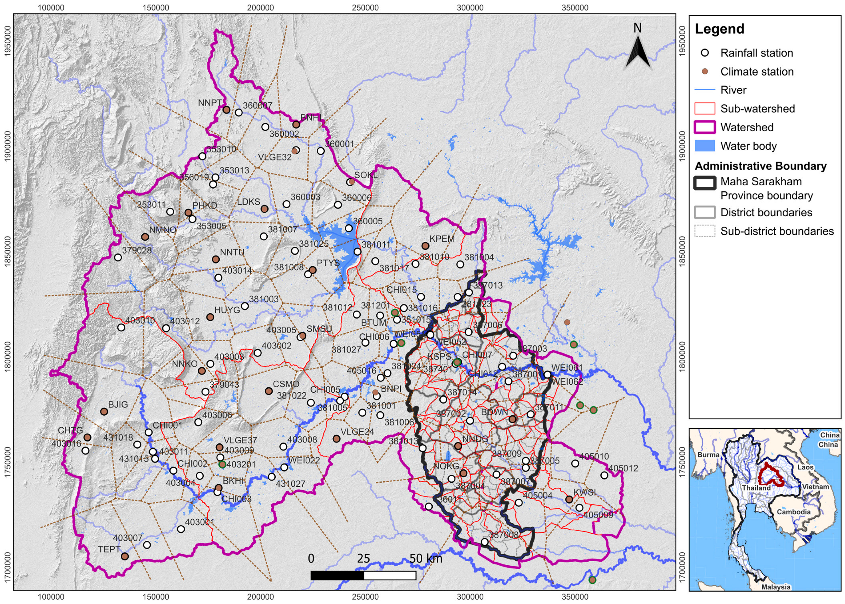
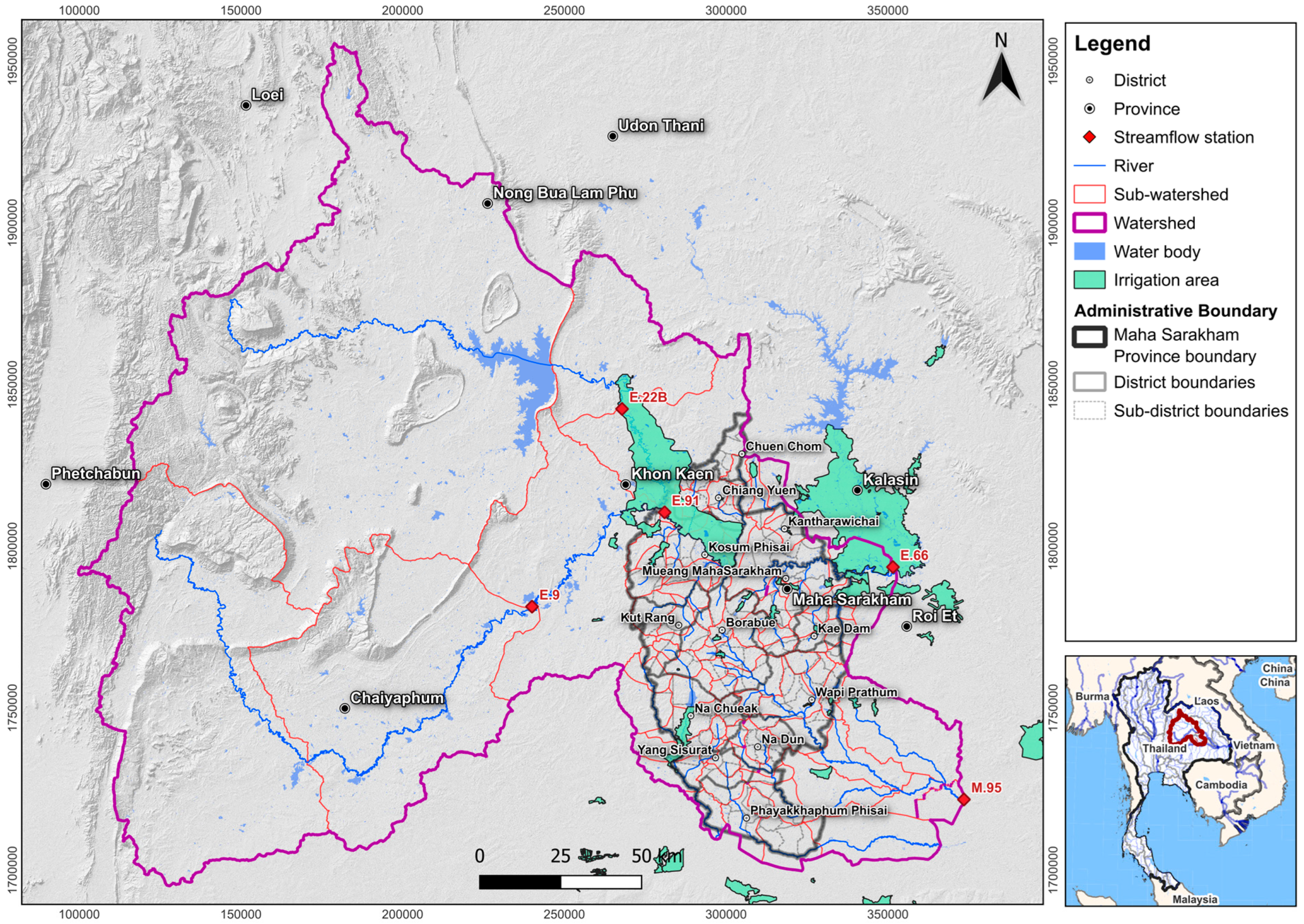
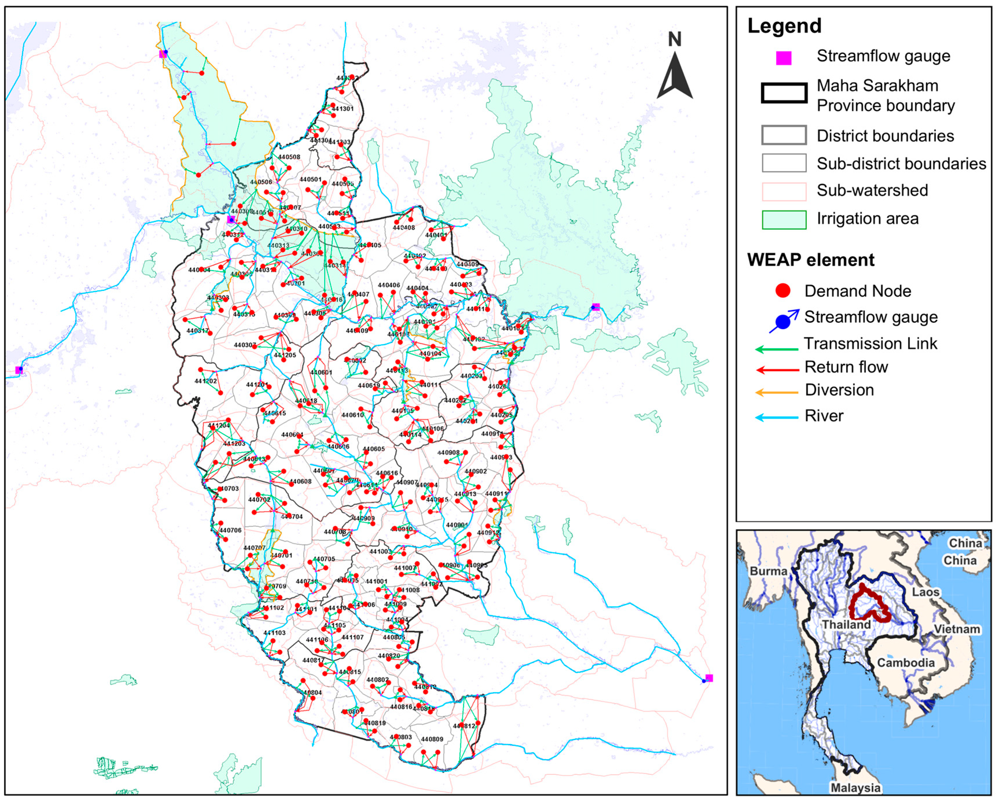
The study area is within the Chi–Mun River system in Northeastern Thailand (see Figure 1), including diverse topographic features (mostly the Korat Plateau) with elevation ranging from 193 to 371 m above mean sea level (MSL). On the western side, the topographic features include mountains in Phetchabun Province, with elevation from 729 to over 1622 m above MSL. Its hydrologic network is composed of two main rivers: the Chi River, originating from a western mountainous area, and the Mun River, which flows through the southern part of the area. Additionally, it consists of two large reservoirs—Ubolrat Reservoir, with a normal storage capacity of 2431.3 MCM and a mean annual inflow of 2957 MCM, and Lam Pao Reservoir, with a normal storage of 1980 MCM—which regulate streamflow in the watershed. There is also a network of six streamflow-monitoring stations (E.9, E.22B, E.91, E.66, M.95, and Ubolrat inflow), which are strategically distributed throughout the watershed to monitor the spatial variability of flow patterns.
The study area has a tropical climate with distinct wet and dry seasons. The mean annual precipitation based on 30-year averages ranges from 1150.0 mm in Chaiyaphum to 1234.5 mm in Khon Kaen and 1315.5 mm in Maha Sarakham, concentrated during May to September. The mean annual temperature is approximately 28 °C, with relative humidity of 71% to 76%. Monthly potential evapotranspiration averages at 154 to 158 mm, indicating that annual evaporative demand exceeds precipitation and creates a water deficit condition. Mean annual streamflow values recorded at stations upstream of Maha Sarakham Province (E.9: 145.0 MCM, E.22B: 143.9 MCM, E.91: 408.4 MCM) and at the downstream station E.66 (484.7 MCM) show strong seasonal concentration during the wet season. This seasonal imbalance between water supply and demand provides the hydrological basis for water scarcity risk assessment and hydrologic modeling using QSWAT.
The study area is underlain predominantly by Mesozoic sedimentary formations of the Korat Group, consisting mainly of sandstone, siltstone, and mudstone, with the Maha Sarakham Formation containing evaporite deposits, including rock salt layers [43]. These geological characteristics result in predominantly sandy loam and loamy soil with limited water retention capacity [44]. The dominant land use is rain-fed rice paddy covering the majority of lowland areas, making agricultural water demand highly dependent on the seasonal rainfall patterns described above.

2.1.2. Administrative Boundaries and Adjacent Areas

The majority of the study area is in Maha Sarakham Province, covering 5292 square kilometers (sq.km) and located in a strategic location where several tributaries within the Chi–Mun system join together. The province borders Khon Kaen Province to the north, Roi Et Province to the east, and Surin Province to the south. It consists of 133 sub-districts, each of which has clearly defined boundaries for systematic assessment and water resource management. Nevertheless, this study area also extends into adjacent provinces which are part of the watershed to ensure that the hydrologic system is fully covered. Administrative boundaries serve as fundamental units to implement water management and availability assessments at the sub-district level.

2.2. Hydrologic Modeling

2.2.1. QSWAT Model

Within the integrated system architecture (Section 2.5), QSWAT serves as the first-stage supply-side component responsible for simulating sub-watershed streamflow from physical and meteorological inputs. The validated streamflow outputs are subsequently transferred to WEAP for water balance analysis at the sub-district level. QSWAT, which integrates the Soil and Water Assessment Tool (SWAT) with QGIS, is a comprehensive hydrologic modeling system designed to simulate hydrologic processes at the watershed level [19]. This integrated model was developed to increase the capacity of and access to hydrologic analysis, and it has been extensively applied in different fields for purposes such as fluid dynamics assessment, sediment yield analysis, and analyses of the impacts of land use and climate change on water resources [20,21,22,28,29,30]. The model is founded on hydrologic principles, using water balance equations to calculate changes in storage as component differences between inflows and outflows; furthermore, it uses an energy balance approach for evapotranspiration modeling. Recent applications have demonstrated diverse uses of QSWAT in different geographic and hydrologic contexts, including for runoff and erosion assessment [45,46], flood risk model development [47,48], and efficiency improvement of watershed management [49], emphasizing the potential of the model in terms of its accuracy and adaptability. Water balance in QSWAT is determined via Equation (1):
SW total   =   SW 0   +   i = 1 t ( R d     Q s     E a     w seep     Q gw )
where SWtotal is the soil water content at time t (mm); SW0 is the initial soil water content (mm); t is the time (unit: day); Rd is the daily cumulative rainfall on day i (mm); Qs is the cumulative runoff on day i (mm); Ea is the actual evapotranspiration on day i (mm); wseep is the infiltration on day i (mm); and Qgw is the groundwater content on day i (mm).
SWAT simulates hydrological processes through two sequential phases: the land phase and the routing phase [50,51]. In the land phase, the soil water balance is computed at the HRU level using Equation (1), which partitions daily rainfall into surface runoff, evapotranspiration, percolation, and groundwater recharge. When the soil water content exceeds the soil storage capacity, excess water is converted into three flow components: surface runoff (Qsurf), lateral subsurface flow (Qlat), and groundwater return flow (Qgw,return). In the routing phase, these components are aggregated at each sub-watershed outlet and routed through the channel network to produce simulated streamflow (Qstream), expressed via Equation (2):
Q stream   =   Q surf   +   Q lat   +   Q gw , return
Accordingly, Equation (1) does not compute streamflow directly but serves as the governing equation from which the streamflow components in Equation (2) are derived. Specifically, Qs in Equation (1) corresponds to Qsurf, and the groundwater component (Qgw) contributes to baseflow through the shallow aquifer return flow process.

2.2.2. Data Collection

Necessary inputs for QSWAT were obtained from different government organizations, including physical watershed features, meteorological parameters, hydrologic measurements, and operational data from Ubolrat Reservoir (Figure 1). The input data listed in Table 1 encompass two categories with different temporal characteristics. Static spatial data, including the DEM (2019), soil-type map, and land-use map (2019), represent quasi-static variables that change gradually over time, with substantially lower variability compared to meteorological and hydrological time series [52]. The most recent datasets available from government agencies were selected to represent these variables. All time-series data, including meteorological parameters, streamflow observations, and reservoir operational records, cover the same 14-year period (2010–2023) and were harmonized to the monthly computational time step of QSWAT. Model calibration against observed monthly streamflow values using SWAT-CUP/SUFI2 was performed to ensure that the simulated outputs accurately approximate actual hydrological conditions [53].

2.2.3. Sub-Basin Delineation

The study area is located in Maha Sarakham Province, covering part of the Chi and Mun Basins. The Chi Basin has four sub-watersheds, including Chi Watershed 3, Chi Watershed 4/1, lower Phong Watershed 2, and Lower Lam Pao Watershed. For sub-watershed division of the Chi watershed in QSWAT, the source of the Chi River and the catchment area of Ubolrat Reservoir must be considered. The Mun Basin also has four sub-watersheds, including Lam Siao Yai Watershed 1, Lam Phang Chu Watershed, Lam Plapphla Watershed, and Lam Tao Watershed, all of which are tributaries of the Mun River. In QSWAT, however, division of the Mun Watershed into additional sub-watersheds is unnecessary. For sub-watershed analysis in QSWAT, DEM data are integrated with available stream network data. This process resulted in 90 sub-watersheds obtained for the study area, consistent with the sub-district administrative boundaries shown in Figure 1.

2.2.4. Importing Rainfall and Meteorological Data

Rainfall and meteorological data covering the divided sub-watersheds described in Section 2.1.1 were used as input variables for the QSWAT model, and model calibration and validation were performed by comparing simulated monthly streamflow values with data obtained from the six monitoring stations. Data obtained from the Thai Meteorological Department (TMD) and the Hydro-Informatics Institute (HII) include 111 rainfall monitoring stations, 34 temperature monitoring stations (minimum and maximum), 34 relative humidity monitoring stations, 8 wind speed monitoring stations, and 5 solar radiation monitoring stations. Daily data over a 14-year period (2010–2023) were analyzed. Spatial distributions of meteorological variables for each sub-watershed were identified using the Thiessen polygon method, as shown in Figure 2.

2.2.5. Importing Hydrologic Response Units

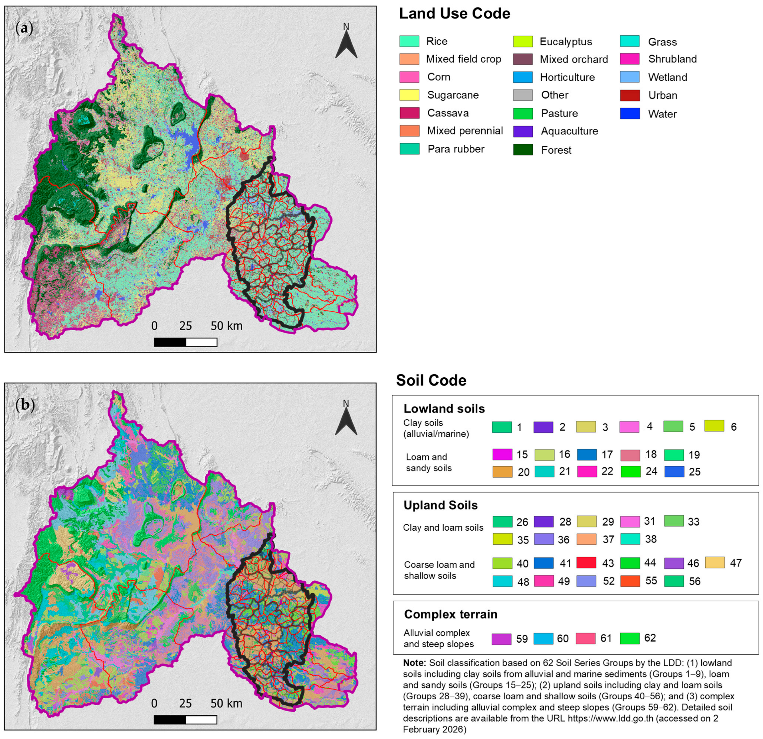
Watershed areas exhibit spatial variability in land use, soil types, slope, and land management, each with distinct hydrologic parameters—such as curve number (CN)—that lead to different hydrologic outcomes [20,54]. In this study, QSWAT employed a spatial analysis tool in QGIS including three layers of GIS data: land-use data (19 types) and soil-series data (41 types), both recorded by LDD in 2019, and slope classification (3 classes) derived from DEM. Hydrologic Response Units (HRUs) were defined by unique combinations of land use, soil type, and slope class within each sub-basin, following the standard SWAT methodology. Default area percentage thresholds in QSWAT were applied for land use, soil, and slope to filter out HRUs with areas too small to contribute meaningfully to the model’s behavior, which is a widely accepted practice in SWAT applications. This process resulted in the attainment of 414 HRUs across the 90 sub-basins. This relatively modest number of HRUs reflects the physical characteristics of the study area: the watershed is predominantly located on the Korat Plateau with elevations ranging from 193 to 371 m MSL, resulting in flat terrain with minimal slope variation, while land use is dominated by rice paddies, thus limiting the effective number of unique combinations. The detailed land-use map and soil-series inputs for the model are presented in Figure 3a and b, respectively.

2.3. WEAP Model

The Water Evaluation and Planning System (WEAP) model receives the validated streamflow outputs from QSWAT as a water supply input, which is then combined with water demand data from four consumption sectors to perform water balance analysis at the sub-district level. This integration completes the scale transformation from hydrological sub-watershed boundaries to administrative jurisdictions, as described in the system architecture (Section 2.5). WEAP was developed at the Stockholm Environment Institute (SEI) in 1988 and serves as an integrated tool for water resource planning and assessment [32]. The model requires basic data regarding hydrology, meteorology, water resources, water demand, and water infrastructure in the study area. It has been globally used due to its capacity to simulate complex water resource systems, analyze water management policy, and enable simulations to assess water management options. The model’s flexibility allows its parameters and conditions to be easily adapted to assess the impacts of climate change, land-use change, and/or water infrastructure development in order to analyze priority-based water allocation and conduct water scarcity risk assessments by sector [32,33,34,35,36,37,38,39]. The WEAP model can be integrated with other hydrologic models such as SWAT, using the simulated streamflow as water resource data for water balance analyses and scarcity assessments [33,55,56]. Moreover, its compatibility with groundwater models and water quality data allow for comprehensive quantitative and qualitative analyses, yielding results with higher precision and reliability.
WEAP uses four basic equations for water balance modeling and water scarcity analysis [56], including Equation (3) for mass balance of water volume change in a system, Equation (4) for water balance at the node for storage volume change, Equation (5) for water demand calculation inclusive of efficiency and area, and Equation (6) for water scarcity, as specified by the difference between demand and supply.
dV dt   =   Q in     Q out
S ( t + 1 )   =   S ( t ) + I ( t )   +   O ( t )
W D   =   AWR   ×   ( 1 e f )   ×   A L
W S   =   W D W A  
where dV/dt is the rate of water volume change rate per time in the system; Qin is the volume of water flowing into the system; Qout is the volume of water flowing out of the system; S(t+1) and S(t) are the storage volumes at time t + 1 and t, respectively; I(t) is the water content flowing in at time t; O(t) is the water content flowing out at time t; WD is the water demand; AWR is the rate of water demand per unit area; ef is the water use efficiency; AL is the water-consuming area; and WS is the water scarcity.
WEAP requires three main types of input—(1) water supply data, (2) spatial data, and (3) water demand data (Table 2)—including seven components: (1) demand site node, (2) flow requirement node, (3) reservoir node, (4) river, (5) transmission link, (6) return flow, and (7) streamflow gauge. Imported GIS data, as the background data of the model, include watershed boundary, river network, water source, streamflow gauge, irrigation area, road, and sub-district boundary information, as shown in Figure 4 and Figure 5. In addition to the water balance equations, WEAP requires land use parameters for hydrological simulation. The four most sensitive parameters in the WEAP model are soil water capacity (SWC), runoff resistance factor (RRF), crop coefficient (Kc), and root zone conductivity (RZC) [57]. SWC controls the volume of water stored in the soil profile, directly affecting evapotranspiration, runoff, and interflow, and is set at 500.0 mm for agricultural areas. RRF governs the fraction of rainfall that becomes direct runoff, which is set at 2.0 for agricultural areas, reflecting the moderate infiltration capacity of cultivated land. Kc determines crop evapotranspiration demand on a monthly and seasonal basis, which is set at 0.88, corresponding to rice-dominated cultivation in the study area. RZC controls the rate of water movement from the root zone, influencing soil moisture and flow timing, which was set at 20.0 mm per month. The variables in Equations (3)–(6)—namely AWR, ef, and AL for water demand calculation, as well as reservoir operational parameters including storage capacity, storage–elevation curve, evaporation rate, and operation rules—serve as the key input parameters for the WEAP model, which were obtained from government agencies as detailed in Table 2.

2.4. Model Performance Assessment

The efficiency of the QSWAT and WEAP models were assessed using three statistical indices. For the assessment of QSWAT, we calculated the Coefficient of Determination (R2) to identify the correlation between measured and modeled streamflow values (Equation (7)), the Nash–Sutcliffe Efficiency (NSE) to measure model’s forecast precision compared to the observed mean (Equation (8)), and ratio of the RMSE to the standard deviation of observed values (RSR) (Equation (9)). The assessment covered calibration (2010–2016) and validation (2017–2023) phases, each spanning 7 years. Notably, the calibration (2010–2016) phase included a one-year warm-up period (2010) to allow hydrological state variables to reach equilibrium, followed by six years of effective calibration (2011–2016).
On the other hand, WEAP verification followed a distinct procedure from QSWAT calibration. WEAP received the validated streamflow outputs from QSWAT as water supply inputs, rather than simulating streamflow independently. This coupled modeling approach—where a calibrated hydrological model provides streamflow inputs for WEAP’s water allocation analysis—is consistent with recent studies on integrated water resources [58]. The WEAP model distributes available water supply to demand nodes using a built-in linear programming algorithm based on demand priorities and supply preferences [59]. Therefore, WEAP does not require parameter calibration in the conventional hydrological modeling sense. The monthly streamflow values computed with WEAP for four monitoring stations (E.9, E.91, E.66A, and M.95) were compared against corresponding observed monthly streamflow records over the full 14-year period (2010–2023), for a total of 168 data points per station. R2 and NSE were calculated using Equations (7) and (8), where Oi represents the observed monthly streamflow and Pi represents the monthly streamflow computed with WEAP for each station. These performance indicators are widely adopted in WEAP-based studies to evaluate the agreement between modeled and observed streamflow values [57,59,60]. This procedure constitutes verification of the WEAP water balance framework’s internal consistency, rather than evaluating its capacity for independent hydrological simulation. Statistically reliable criteria were used for calibration of the monthly model, in order to assess its precision and accuracy [61]:
R 2   =   i = 1 n ( O i O ¯ ) ( P i P ¯ ) i = 1 n ( O i O ¯ ) 2 i = 1 n ( P i P ¯ ) 2
NSE   =   i = 1 n ( O i O ¯ ) 2 i = 1 n ( P i P ¯ ) 2 i = 1 n ( O i O ¯ ) 2
RSR = i = 1 n ( O i P i ) 2 i = 1 n ( O i O ¯ ) 2  
where Oi is the streamflow content recorded at the streamflow gauge; Ō is the average streamflow content recorded at the streamflow gauge; Pi is the streamflow content calculated using QSWAT or WEAP; P ¯ is the average streamflow content calculated using QSWAT or WEAP; and i indexes the data sequence.

2.5. Integrated Water Balance Assessment Framework

2.5.1. System Architecture and Integration Framework

Local administrative organizations, including Sub-district Administrative Organizations (SAOs) and municipalities, possess legal authority and budgetary autonomy to allocate resources for local water management, including water source development, water supply systems, and drought mitigation. However, hydrological data produced by national water agencies are available only at the watershed scale, which local administrative organizations cannot directly apply for sub-district-level planning. This limitation particularly affects sub-districts located outside irrigated zones or those lacking water infrastructure. The proposed system was therefore designed to bridge this institutional gap.
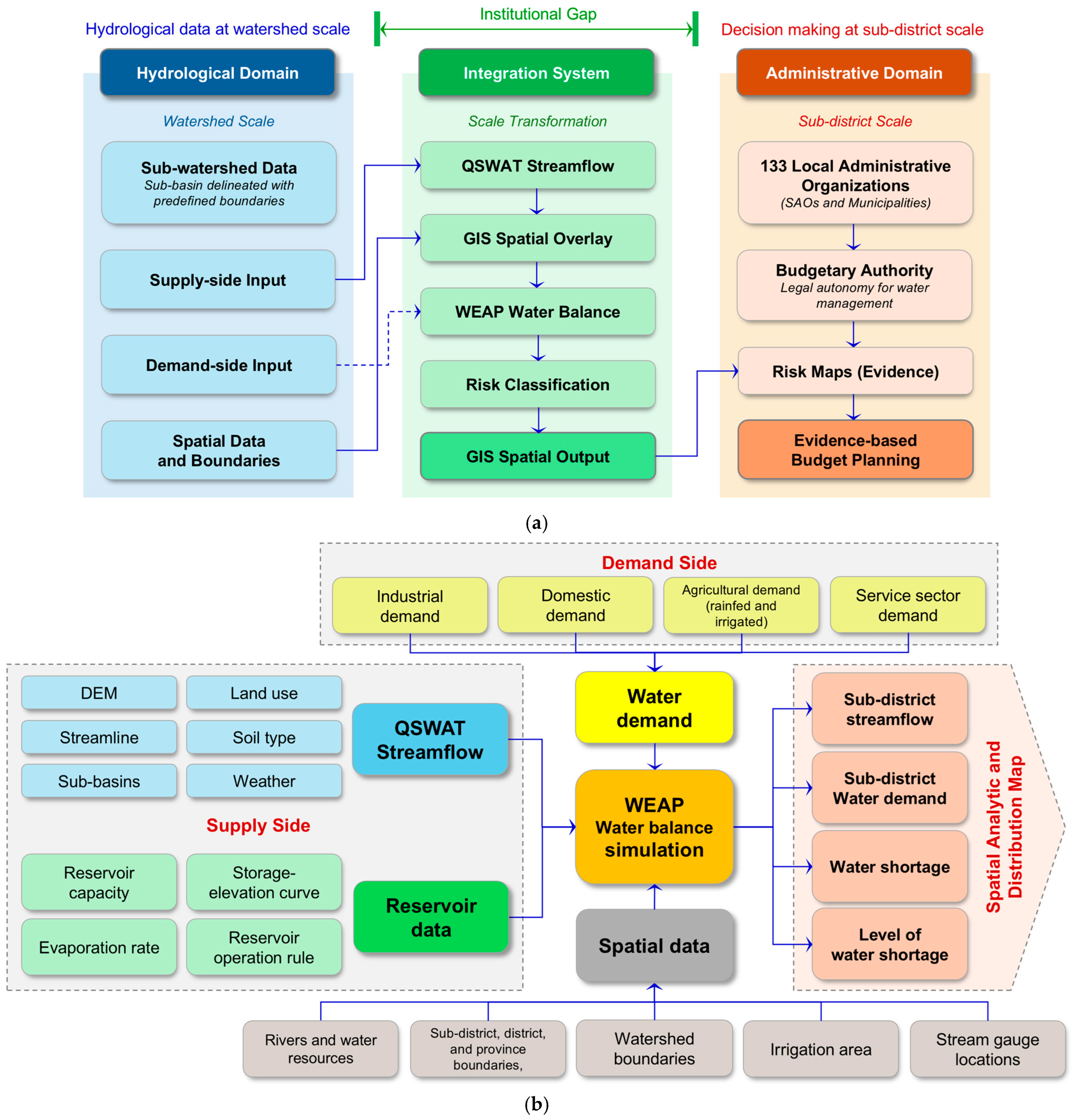
The system architecture (Figure 6a) is organized into three domains: (i) the Hydrological Domain, where streamflow is simulated from 90 sub-watersheds at the watershed scale; (ii) the Integration System, which performs scale transformation from watershed level to sub-district level through QSWAT streamflow simulation, GIS spatial overlay with area-proportional allocation, and WEAP water balance analysis with risk classification; (iii) the Administrative Domain, where 133 local administrative organizations in Maha Sarakham Province can use the resulting risk maps as evidence for relevant planning.
The data flow follows a unidirectional sequence through five components: (1) the Input Data Layer with separate supply-and-demand streams, (2) QSWAT Hydrological Simulation, (3) WEAP water balance analysis, (4) a Risk Classification Module, and (5) GIS Spatial Output. A key design feature is that demand data bypass QSWAT and enter WEAP directly, as water demand is calculated at the level of administrative units rather than hydrological units. Furthermore, the independence of each component allows for selective updating, such as incorporating new land-use data or revised demand projections, without requiring full system recalibration.

2.5.2. Detailed Framework for Water Balance Simulation

The detailed framework (Figure 6b) illustrates the data-processing procedures within the integrated system described in Section 2.5.1. On the supply side, QSWAT receives primary inputs including DEM, land use, river network, soil type, sub-watershed boundaries, and meteorological data, together with reservoir data (including storage capacity, storage–elevation curve, evaporation rate, and reservoir operation rules). These data are processed to simulate daily streamflow for each sub-watershed using Equation (1), with parameters calibrated via SWAT-CUP/SUFI2. The predefined watershed delineation approach ensures that sub-watershed boundaries correspond to sub-district administrative boundaries, which provides the essential basis for scale transformation in the subsequent steps.
On the demand side, as shown in the upper portion of Figure 6b, water demand data from four sectors—namely industry, domestic consumption, agriculture (both irrigated and rain-fed areas), and services (Table 2)—are combined with spatial data including water sources, administrative boundaries, watershed boundaries, irrigation zones, and stream gauge locations for water balance simulation in WEAP using Equations (2)–(5). These demand data are input to WEAP directly without passing through QSWAT, following the design principle described in Section 2.5.1.
The simulation results, displayed on the right side of Figure 6b, include four types of spatial output at the sub-district level: Streamflow distribution, water demand distribution, water shortage, and level of water shortage (classified into five severity levels). These maps serve as the final outputs of the system, which are delivered to the Administrative Domain such that each local administrative organization can identify its own water scarcity situation and use this evidence to support targeted budget allocation decisions.

2.5.3. Water Scarcity Evaluation Metrics

Following the system architecture and integration framework described in Section 2.5.1 and Section 2.5.2, the final outputs of the integrated QSWAT and WEAP system are provided as four complementary evaluation metrics. Fundamentally, the water scarcity risk assessment is based on the concept that water scarcity occurs when water demand exceeds the available water supply in a given area and time period. Accordingly, rather than developing a new composite index, these metrics are computed at sub-district administrative resolution with monthly temporal detail to capture the spatial and temporal dimensions of water scarcity.
Specifically, water availability (WA) represents the total streamflow within each sub-district boundary, derived from QSWAT-simulated sub-watershed discharge allocated to 133 administrative units through GIS area-proportional overlay. Subsequently, water demand (WD) is computed using Equation (4) by aggregating the demands of four sectors: Agriculture, domestic consumption, industry, and services. Based on these two components, water shortage (WS) is then calculated as the difference between total water demand and available water supply (Equation (5)). This metric serves as the primary evaluation indicator, as it directly quantifies the magnitude of water deficit for each sub-district on a monthly basis. Furthermore, the level of water shortage expresses the water shortage as a percentage of total water demand, thereby providing a normalized measure that enables comparison among sub-districts with different demand magnitudes.
To facilitate interpretation, the water shortage and level of water shortage values are classified into five risk levels, representing the spatial distribution of water scarcity severity across the study area. The classification thresholds were defined by the authors based on the distribution of data in the study area and expert judgment, considering local water management conditions. Consequently, each sub-district is assigned a distinct risk category that can be directly interpreted by local administrative organizations for water management planning.

3. Results and Discussion

3.1. Streamflow Simulation from QSWAT

3.1.1. Parameter Sensitivity Analysis

Sensitivity analysis of QSWAT was conducted using SWAT-CUP through Sequential Uncertainty Fitting version 2 (SUFI2) [62], in order to analyze the effects of parameters on the calculated streamflow in comparison to 14-year (2010–2023) monthly streamflow data obtained from the six monitoring stations. To obtain comparable results to the measured value, optimization was performed for 300 iterations after selecting 14 parameters affecting the streamflow [28] and defining the Nash–Sutcliffe efficiency (NSE) as an objective function. The global sensitivity analysis results obtained with SWAT-CUP are expressed as t-statistics and p-values obtained from hypothesis testing of the relationships between parameters and the objective function. This analysis indicated that the leading three parameters affecting the calculation results were GWQMN (3537), SOL_AWC (0.07), and GW_REVAP (0.83); in particular, these parameters showed absolute t-statistics and p-values approaching zero, indicating significant sensitivity to the objective function [63]. The remaining 11 parameters, showing low sensitivity, are ranked and presented in Table 3.

3.1.2. Performance Assessment of Models

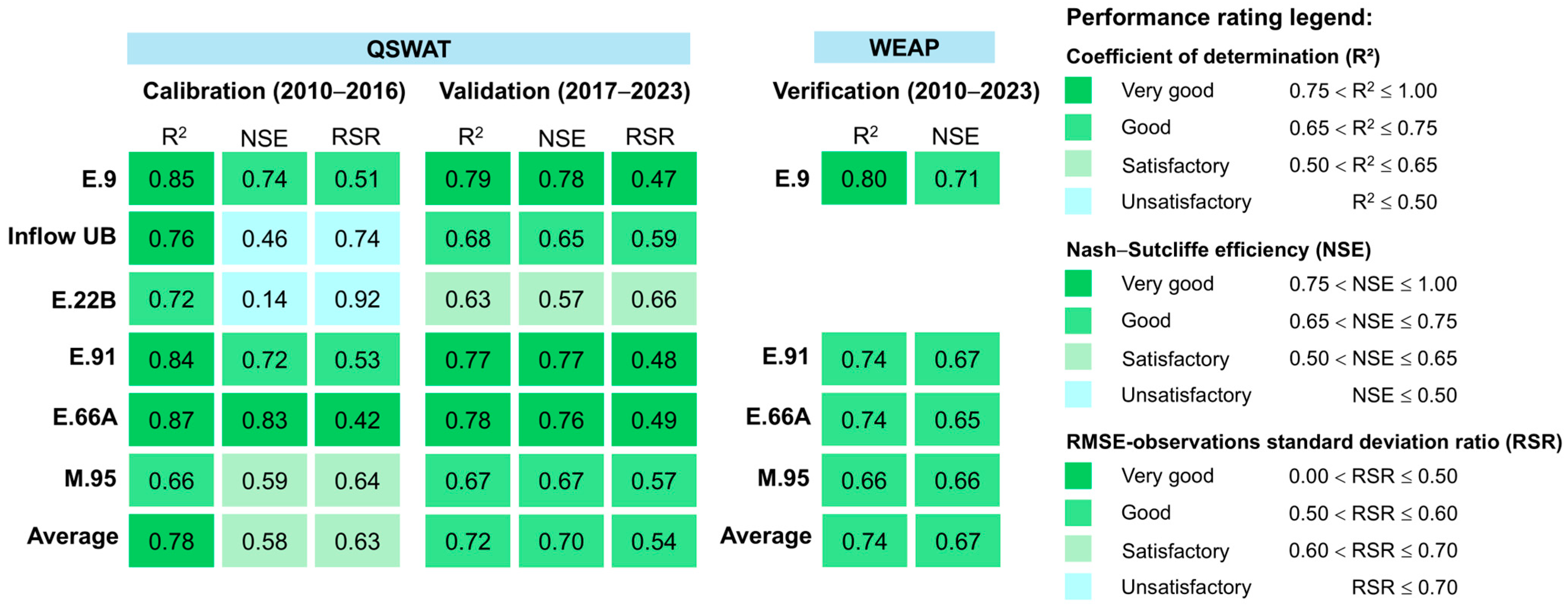
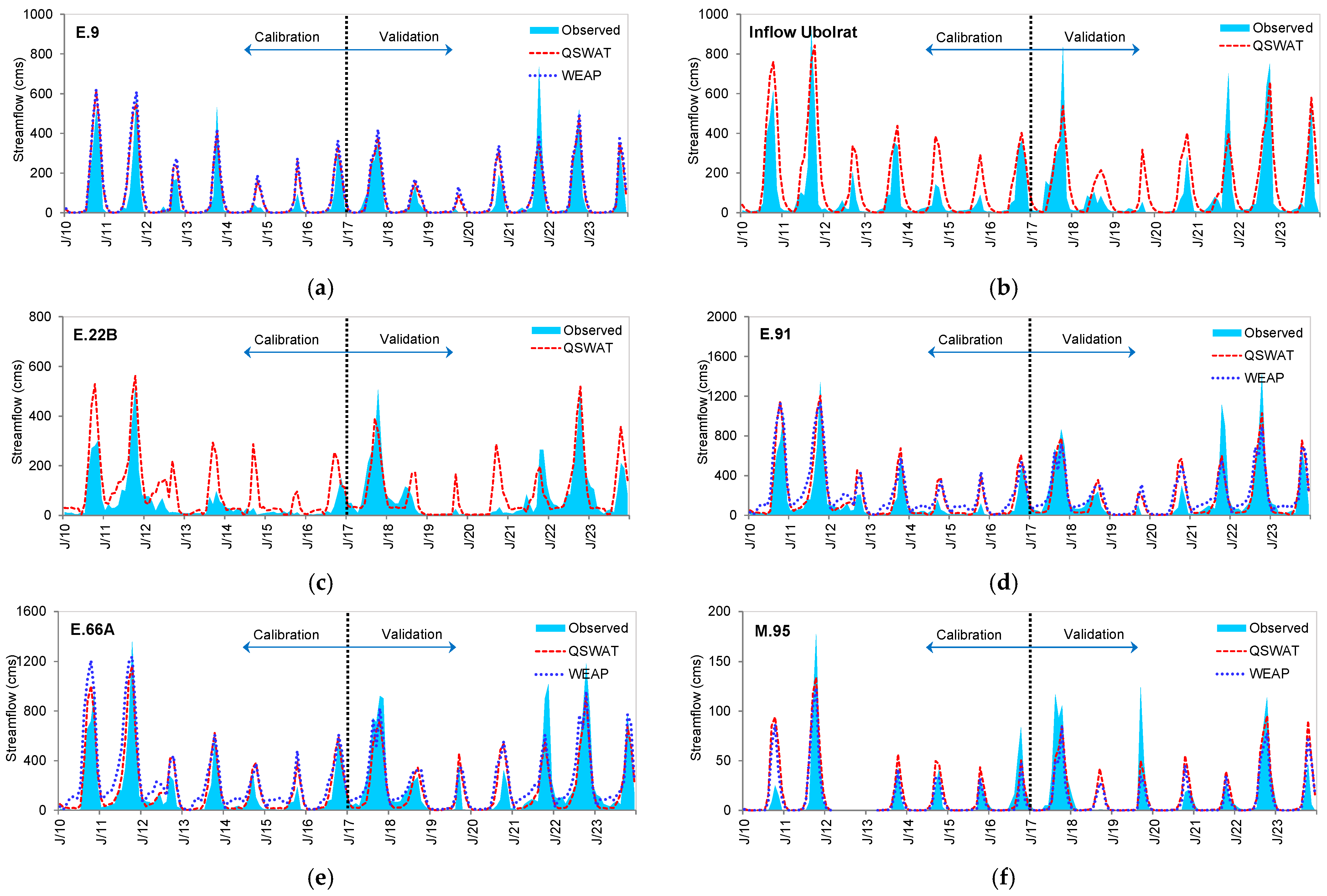
The performance assessment results for the QSWAT and WEAP models are illustrated in Figure 7 as heat map indices, as well as in Figure 8, which represents the consistency of monthly streamflow data from monitoring stations and the calculation results obtained from the time series model for the six stations during the period 2010–2023. According to the QSWAT results for the calibration period (2010–2016), most stations had R2 values between high and very high levels (0.66–0.87). Station E.66 had the highest level (0.87). The NSE was between 0.14 and 0.83; notably, station E22B and Ubolrat Reservoir (Inflow UB) had values below the satisfactory range (at 0.14 and 0.46, respectively). Periods of low streamflow were noticed at both stations. The values obtained from the models were higher than the observed values, as shown in Figure 8b,c; however, based on the average of all six stations, the NSE was at a satisfactory level (0.58). The RSR index was consistent with the NSE (0.63), which was satisfactory. In the model validation period (2017–2023), each index showed better outcomes. Stations E9, E91, and E66 obtained very good results, according to the three indices. The remaining stations were at good and satisfactory levels (average R2 = 0.72, NSE = 0.70, and RSR = 0.54).
Performance assessment of streamflow in WEAP was conducted to verify that the streamflow outputs from QSWAT, when routed through the WEAP water allocation framework, remained consistent with the observed data at four key monitoring stations. In WEAP, the streamflow of main river, which flows through the study area and becomes potentially applicable, enabled water balance analysis in three parts: (1) Water availability, (2) water demand, and (3) sub-district-level water shortage in Maha Sarakham Province. In this assessment, the R2 and NSE indices were used for four main stations (E.9, E.91, E.66A, and M.95). The first three stations were considered with the aim of monitoring streamflow in the Chi River, affecting northern Maha Sarakham Province. On the other hand, M.95 enabled performance assessment for Lam Siao River, located to the south and outside of Maha Sarakham Province. The verification results showed that streamflow within the WEAP water balance framework maintained acceptable agreement with the observed data from the four stations, with R2 between 0.66 and 0.80 and NSE between 0.65 and 0.71, and maintained temporal consistency for the period 2010–2023, as presented in Figure 8a,d–f. The averages of both indices were at a good level, and the optimal models ranked by performance were those for E.9, E.91, E.66, and M.95. The overall performance assessment for QSWAT and WEAP demonstrates that the streamflow stimulated by both models provided reliable data (at a satisfactory-to-good level), in terms of model accuracy and temporal data consistency.

3.2. Spatial Distribution of Water Resources

3.2.1. Sub-District Streamflow Analysis

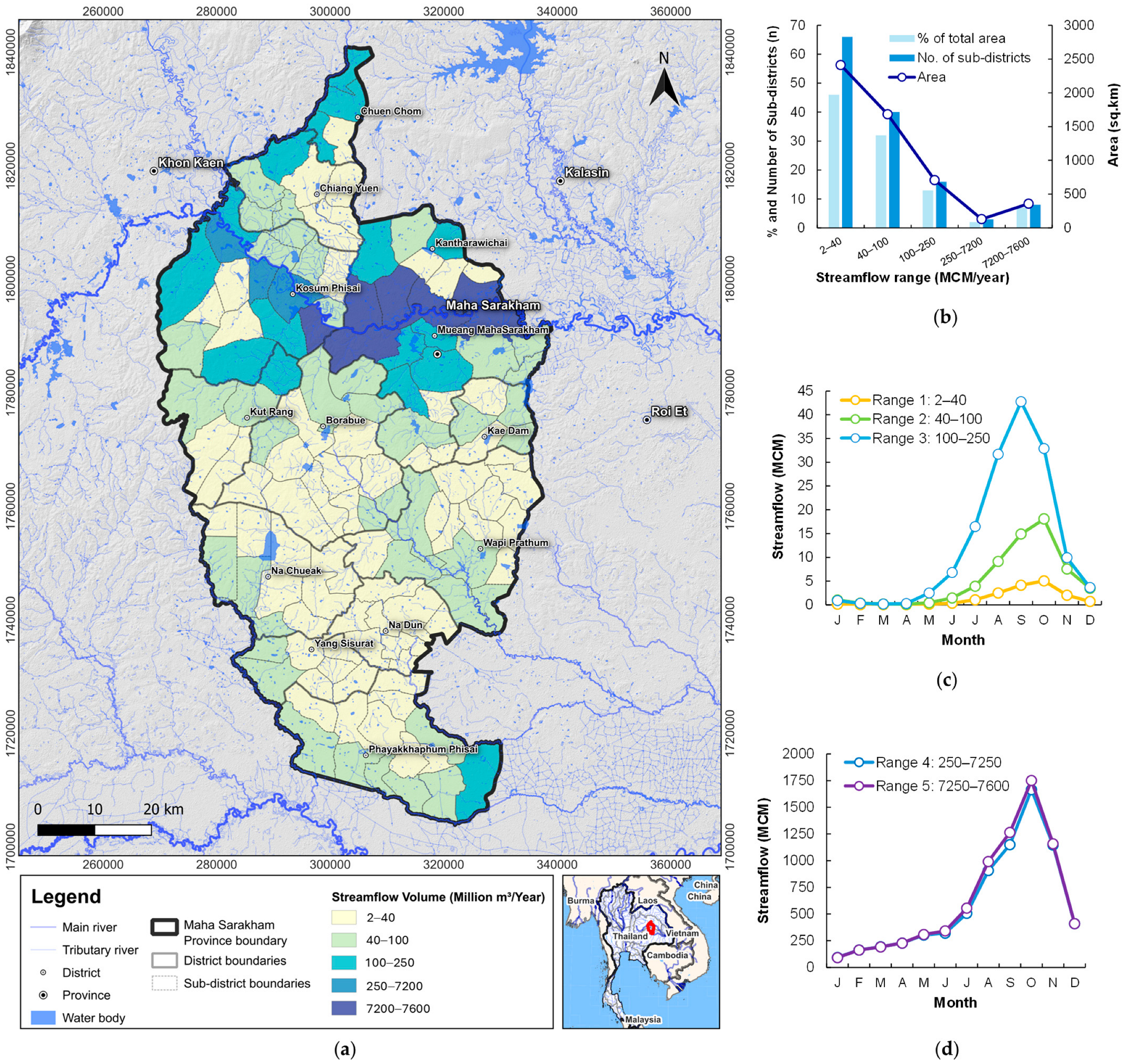
The streamflow analysis results obtained with QSWAT and WEAP for the period 2010–2023, as shown in Figure 9a, were classified into five levels of spatial distribution. Sub-districts located near the Chi River—which is a main river flowing through the northern and central parts of the province (represented by dark blue in the map)—demonstrated high-to-very high streamflow (Ranges 4–5: 250–7600 MCM per year) due to surface runoff over the sub-district areas and the influence of water from the main river. On the other hand, southern and southwestern sub-districts in the province (represented by light green), which are far from the main river and rely only on surface runoff in the area, had low streamflow (Range 1: 2–40 MCM per year). Analyzing the quantitative data (see Figure 9b), Range 1 covers 2212 sq.km (or 46%) of the total area, including 66 sub-districts; while Range 5 covers only 359 sq.km (or 8%) of the total area, including 7 sub-districts. Meanwhile, Ranges 2–4 cover 2521 sq.km (or 47%), including 59 sub-districts (40, 16, and 3 sub-districts, respectively) distributed in the central part of the province, which is a border area between the main river and areas remote from the river.
The analysis of monthly streamflow changes, as shown in Figure 9c,d, revealed seasonal changes consistent with the spatial distribution in Figure 8a. Ranges 1–3 (Figure 9c) had low streamflow, reaching its maximum during September–October with 4.2–42.7 MCM and minimum during February–April with 0.02–0.28 MCM. This is represented as the light yellow, light green, and light blue areas in the distribution map, covering 122 (or 91%) of the total sub-districts. In case of Ranges 4–5, as shown in Figure 9d, the maximum streamflow was 1665.5–1750.3 MCM in October and the average streamflow in the dry season (December–July) was 94.3–555.6 MCM, represented by the light and dark blue areas along the Chi River in the distribution map.
According to the spatial streamflow distribution analysis corresponding to area size, the number of districts, and monthly temporal changes in Maha Sarakham Province, the results indicated seasonal imbalance and limited streamflow in the dry season. In contrast, intensity became high in the rainy season, which was significantly consistent with the spatial contribution and geographical characteristics of Maha Sarakham Province. In the dry season, the areas with 0–100 MCM per year (Ranges 1–2), covering 2047 sq.km area (78% of the total area) including 106 out of 133 sub-districts, indicated low monthly streamflow that reflected the widespread distribution of sub-district-level drought. Areas in the central streamflow range (100–250 MCM per year) covered 709 sq.km (or 13% of the total area). The areas with high streamflow (250–7600 MCM per year), which were mostly located near the Chi River, covered 489 sq.km and included only 11 sub-districts, and they showed an obviously higher value from June to October. This imbalance reflects that the area between the central and southern parts of the province had low level of monthly streamflow change, while not many northern sub-districts showed a very high intensity of streamflow in the rainy season. The significant differences in streamflow between areas close to and far from the main river reflect the key role of the Chi River as a major water resource of the province, as well as the influence of Ubolrat Reservoir in controlling streamflow in the dry season. This is consistent with the findings of He et al. [64], who indicated that areas far from the main water resource in the Mekong watershed normally encounter water shortages, and Cheng et al. [65], who highlighted that the distance from a main river is a key factor affecting the availability of local water resources.

3.2.2. Sub-District Water Demand Analysis

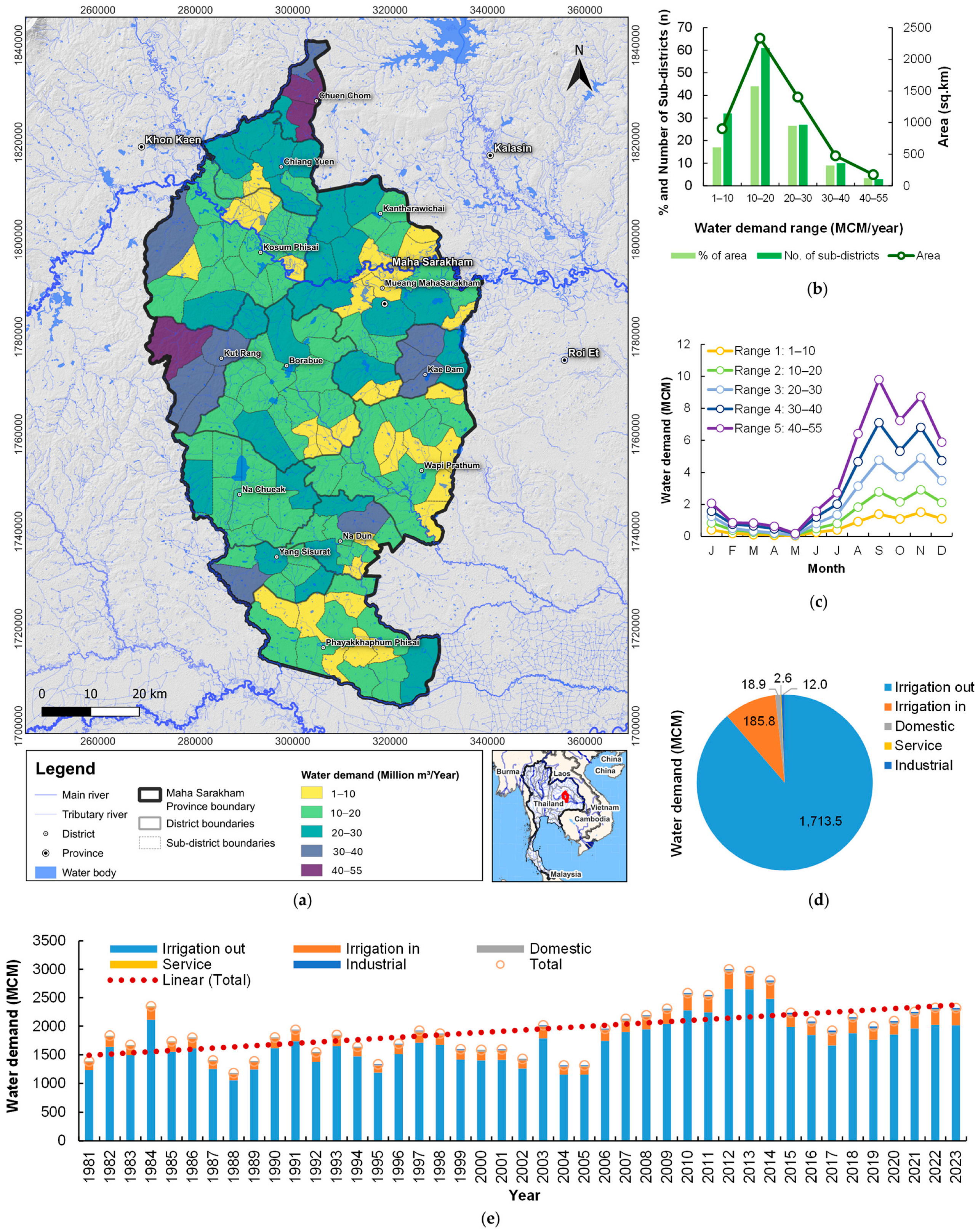
As shown in Figure 10a,b, water demand at the sub-district level, determined using WEAP, was analyzed based on five activities—non-irrigated agriculture, irrigated agriculture, consumption, services, and industry—and divided into five levels. Most of the sub-districts in the province were at level 1 of water demand (1–10 MCM per year), including 32 sub-districts and covering 903 sq.km (or 17% of the total area), which were generally distributed outside the province to the north and the east (represented by yellow). There were 98 sub-districts having a medium level of water demand (Ranges 2–4: 10–40 MCM per year) covering 4211 sq.km (or 80%) and distributed in the northern, central, and southern parts of the province. The highest level of water demand (Range 5: 40–55 MCM per year) was found in only three sub-districts covering 178 sq.km (or 3%), which are represented by dark purple in the map. Comparing Figure 9a and Figure 10a, it is important to note that the water demand distribution obviously differs from the streamflow distribution; in other words, sub-districts with high water demand do not need to be close to a main water resource. This inconsistency becomes an important cause of water shortages in areas far from a main river.
Figure 10c presents the change in monthly average water demand, which is in line with the local crop calendar. All sub-districts present water demand starting from June, which is the period characterized by in-season rice cultivation. Sub-districts with level 5 water demand require 9.8 MCM water in August, while those with Range 1 water demand require 1.4 MCM water in the same month. During the dry season (January–May), areas at all levels show significantly lower water demand. The sub-districts with Range 1 have an average water demand of 0.9 MCM per month. Analyzing the proportion of water demand by sector (Figure 10d), non-irrigated agriculture shows the highest proportion, at 1713.5 MCM per year (88.7%), followed by irrigated agriculture (185.8 MCM per year, 9.6%), consumption (18.9 MCM per year, 0.98%), industry (12.0 MCM per year, 0.6%), and services (2.6 MCM per year, 0.13%). Figure 10e demonstrates the trend of annual water demand, which has continually increased from approximately 1500 MCM in 1981 to 2500–3000 MCM in 2023, representing an average annual increase of 1.7%, caused by agricultural area expansion and population growth. The water demand proportion for non-irrigated agriculture of 88.7% reflects that local agriculturists are reliant mainly on rainfall, making them vulnerable to climate change. Considered in conjunction with Figure 9a, the southern sub-districts in Maha Sarakham Province, where the streamflow is low, present moderate-to-high water demand (Ranges 2–4), indicating a supply–demand imbalance that may lead to water shortages.

3.3. Water Shortage Risk Assessment

3.3.1. Sub-District Water Shortage Analysis

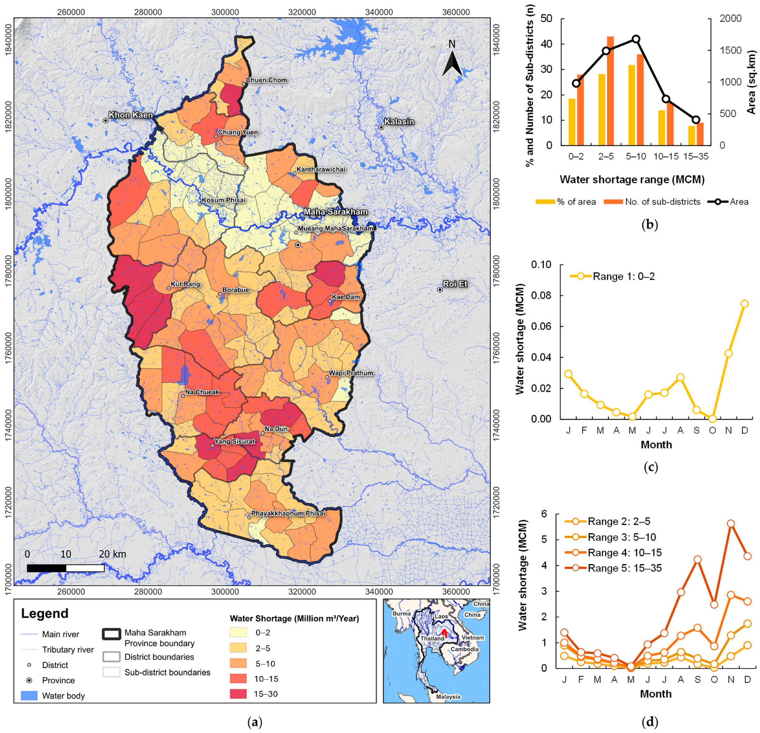
After calculating the difference between water demand and available streamflow for each sub-district, sub-district-level water shortages were assessed and classified into five ranges. As shown in Figure 11a, 28 sub-districts showed the lowest water shortage level (Range 1: 0–2 MCM per year), covering 980 sq.km (or 19% of the total area). These sub-districts are distributed to the north along the Chi River (represented by light yellow) and are thus influenced by high volume of streamflow (Ranges 4–5: 250–7600 MCM per year). Figure 11b presents the 79 sub-districts with moderate water shortage (Ranges 2–3: 2–10 MCM per year) covering 3172 sq.km (or 60% of the total area), distributed widely around the central part of the province. Furthermore, 26 sub-districts faced severe water shortage conditions (Ranges 4–5: 10–35 MCM per year) covering 1140 sq.km (or 22% of the total area), distributed in the south and southwest (represented by dark orange and red). These distributions reflect the imbalances mentioned in Section 3.2.1 and Section 3.2.2; in other words, the southern area has low streamflow (Ranges 1–2: 2–100 MCM per year), while its water demand is at a moderate-to-high level (Ranges 2–5: 10–55 MCM per year).
Figure 11c,d present the monthly changes in water shortage, which obviously differ from those for streamflow and water demand. The sub-districts with Range 1, as presented in Figure 11c, have low constant water shortage throughout the year, with a maximum of 0.07 MCM in December and a minimum of 0.0 MCM in April, May, and October. The sub-districts with Ranges 2–5, as shown in Figure 11d, present maximum water shortages during November–December: 5.63 MCM in November for Range 5 followed by 2.85 MCM for Range 4. All ranges showed a minimum value in May (0.01–0.08 MCM), which is at the beginning of the rainy season. An interesting finding is that the critical period of water shortage (November–December) is not the period characterized by the highest water demand (June–August), as described in Section 3.2.2. On the contrary, streamflow rapidly decreases in the post-harvest period while water demand remains high due to the need to prepare land for the next cycle. This phenomenon indicates that seasonal transitions are critical periods of water shortage in agricultural areas [66], suggesting the importance of water allocation in order of priority during these critical periods [67].

3.3.2. Sub-District Level of Water Shortage Analysis

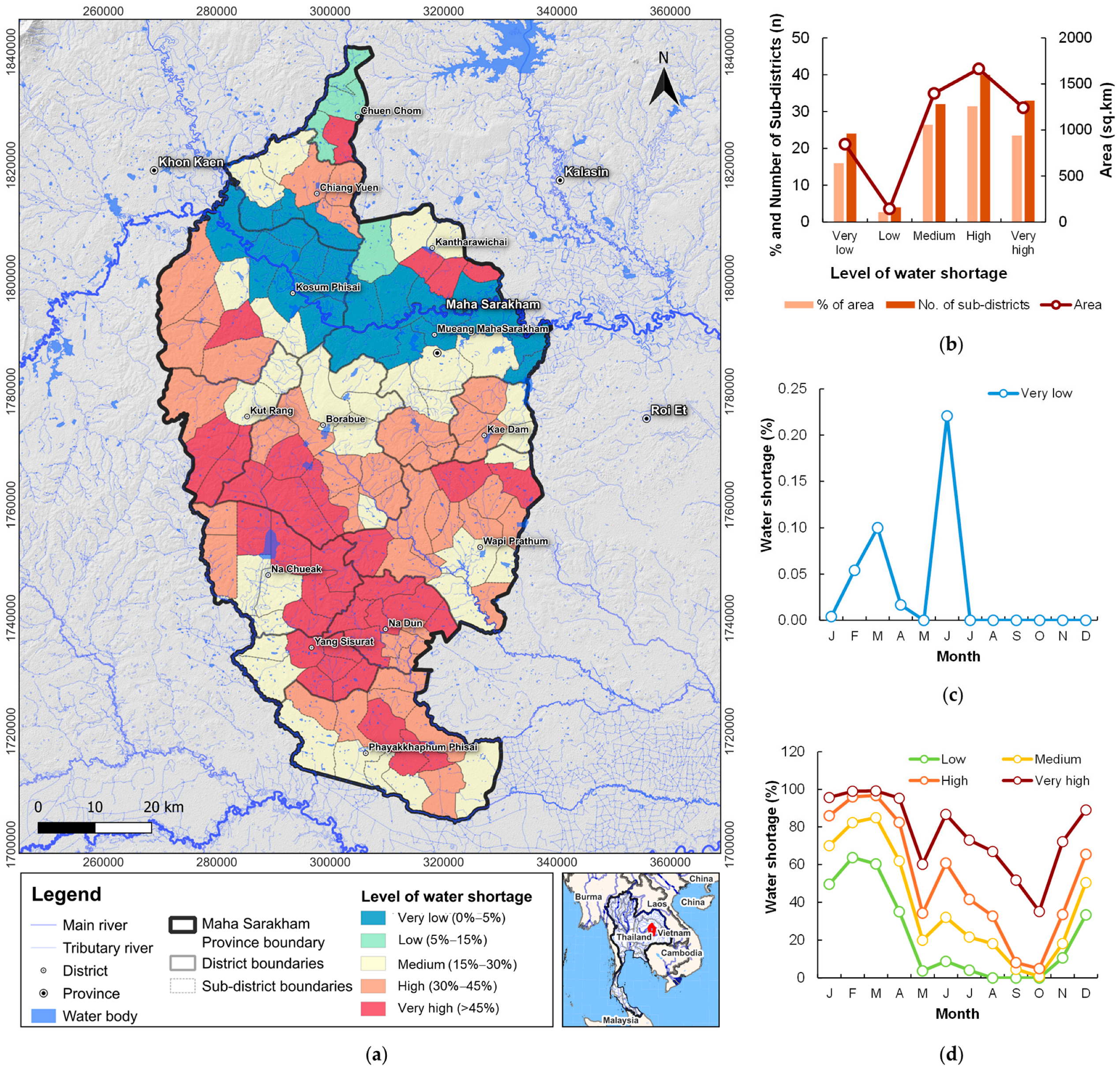
Analyzing the proportion of water shortage severity according to the percentage of unmet water demand can provide more insightful answers than considering only the absolute water shortage (as described in Section 3.3.1), as those sub-districts with low water demand but a high proportion of water shortage are likely more affected than those with high water demand but a low proportion of water shortage. Figure 12a shows the distribution of water shortage severity in five levels. The sub-districts with high severity cover 1664 sq.km (or 31.4%), including 40 sub-districts distributed in the south and east of the province (represented by orange). Secondly, sub-districts with medium severity cover 1397 sq.km (or 26.4%), including 32 sub-districts distributed in the central part of the province. Figure 12b shows the sub-districts with very high severity; although only 33 sub-districts are included, they cover 1242 sq.km (or 23.5%), being distributed in the southernmost and southwestern parts of the province (represented by red) and overlap with the areas with low streamflow (Ranges 1–2 in Section 3.2.1). On the other hand, there were only 28 sub-districts with very low-to-low severity, covering 989 sq.km (or 16%) and being distributed in the north along the Chi River.
The monthly severity changes, as shown in Figure 12c,d, reveal a critical situation for areas with high and very high severity. The sub-districts with very high severity showed 99.24% water shortage in March and severity higher than 95% from January to April. This means that water demand has not been fulfilled throughout the dry season; furthermore, the value remains in the range of 35.23–51.80% in the rainy season, which is still regarded as very high. The sub-districts with high severity show similar results (maximum = 96.82% in March; minimum = 4.96% in October), while those with medium severity have a maximum of 85.00% in March and minimum of 0.79% in October. Those with very low severity present low and constant values throughout the year, with a maximum of only at 0.22% in June. The overall results indicate that there are 105 sub-districts, comprising 79% of the total sub-districts, that are significantly affected (i.e., at a medium-to-very high level) by water shortages; in particular, during January–April, water shortages remain at all levels except the very low level, with shortages reaching higher than 50%. These results suggest that areas in the central and southern parts of the province are urgently in need of measures such as minor water source development, promotion of water use efficiency, and cultivation planning based on water availability.

3.4. Synthesis of Water Balance and Shortage Risk Findings

The water resource distribution (Section 3.2) and water shortage risk assessment (Section 3.3) results jointly represent an obvious relationship between water supply and demand at the sub-district level in Maha Sarakham Province. The study revealed an imbalance between available streamflow and water demand, which significantly differed between the northern and southern parts of the province. The northern area along the Chi River has high streamflow (Ranges 4–5: 250–7600 MCM per year) covering 11 sub-districts and 489 sq.km (9%), leading to very low-to-low severity of water shortage covering 28 sub-districts and 989 sq.km (18.7%). Conversely, the central to southern area is characterized by low streamflow (Ranges 1–2: 2–100 MCM per year) covering 106 sub-districts and 4094 sq.km (78%), and high-to-very high severity covering 73 sub-districts and 2906 sq.km (54.9%). This difference is due to the concentration of main water sources in the north while water demand remains relatively evenly distributed throughout the province; in particular, most sub-districts (101 sub-districts or 76%) had medium-to-high water demand (Ranges 2–5: 10–55 MCM per year), as detailed in Table 4.
Based on the temporal analysis, interesting findings regarding monthly water shortages were revealed. As reported in Section 3.3.1, the maximum water shortage was found during November–December, with the Range 5 area presenting a maximum of 5.63 MCM in November. In Section 3.3.2, it was indicated that areas with a very high level had a 99.24% water shortage in March and shortages higher than 95% from January to April, meaning that water demand was not met in the dry season. After considering the characteristics of each risk level by sub-district (as presented in Table 5), the sub-districts with very high risk had common characteristics: located more than 25 km from a main river, a streamflow intensity below 0.5 MCM per sq.km, dependence on rainwater as a main water source, and a long critical period (from November to June). On the other hand, the sub-districts with very low risk were located near or within five km of the Chi River, had a streamflow intensity over 100 MCM per sq.km, and benefited from the existing irrigation system. These characteristics indicate that distance from a main river and access to irrigation are factors affecting the risk level, which can be used as criteria to screen target areas for the future development of water sources. Overall, the findings support the need to develop minor water sources and local irrigation systems in the south of the province, as well as the promotion of increased water use efficiency in non-irrigated agriculture, which takes up a high proportion (88.7%) of the total water demand.

3.5. General Discussion

The principal methodological contribution of this study is the development of an integrated assessment system that bridges the institutional gap between hydrological modeling boundaries and administrative governance boundaries. Hydrological models such as QSWAT operate at sub-watershed scales delineated by topographic divides, producing outputs that do not correspond to the administrative units where water management decisions and budget allocations are made [40,41]. Previous studies using SWAT–WEAP [16,17,18,33] have typically reported results at the sub-basin level, limiting their direct applicability for local planning agencies. In contrast, this study translates sub-watershed streamflow simulations from QSWAT into sub-district level risk assessments in WEAP through GIS-based overlay with area-proportional streamflow allocation, ensuring that each SAO can directly identify its water shortage severity and prioritize interventions without additional spatial processing.
The open-source platforms and modular architecture (Section 2.5.1) reduce financial barriers for local agencies and allow independent component updates without full system recalibration. The spatial and temporal outputs serve multiple operational levels: policy agencies can utilize severity maps (Figure 12) and sub-district classification (Table 4) for budget prioritization; local administrative organizations can carry out risk factor identification (Table 5) for context-specific drought mitigation; and farmers can apply monthly temporal data (Figure 11 and Figure 12) for crop planning aligned with seasonal water availability. The methodology also offers a transferable framework for other drought-prone regions facing similar institutional gaps between hydrological and administrative boundaries.
The evaluation metrics employed in this study can be compared with the extensive water scarcity indices developed over the past two decades [68,69,70]. These existing indices generally assess water scarcity through per capita availability thresholds, withdrawal-to-availability ratios, or composite scores integrating socioeconomic dimensions. However, they share common limitations; for example, most operate at national or major basin scales with annual temporal resolution, and their outputs have limited applicability to the administrative units responsible for local water management decisions. Consequently, the practical utility of these indices in the context of local governance remains limited. In contrast, the metrics used in this study offer three distinct advantages. First, their sub-district administrative resolution enables each local government unit to interpret its water scarcity status directly without additional spatial processing. Second, the monthly temporal scale reveals critical seasonal periods that annual indices cannot detect, such as the November-to-December transition identified as the peak water shortage period in Section 3.3.1. Third, the metrics are derived from process-based hydrological simulation through the integration of QSWAT and WEAP, rather than from statistical estimation or per capita thresholds. This approach is consistent with recent research emphasizing the need to link water resource analyses with policy decisions at the local governance level.
Nevertheless, this study has certain limitations. First, only surface water was assessed without incorporating a groundwater model. Although SWAT–MODFLOW–WEAP coupling could enhance the system’s comprehensiveness [3,50], the study area is underlain by the Maha Sarakham Formation containing rock salt deposits that produce saline groundwater unsuitable for domestic and agricultural use [71,72], and SAOs primarily manage surface water infrastructure. Furthermore, the integration of groundwater would require detailed hydrogeological parameters and careful consideration of the unique saline characteristics of this region. Second, the impacts of climate change and land-use change were not considered. Future research should explore groundwater model integration in areas with exploitable freshwater aquifers, simulations involving climate change scenarios, and real-time monitoring systems for proactive drought management.

4. Conclusions

The water scarcity risk assessment system developed in this study employs an integrated QSWAT, WEAP, and GIS architecture, which was designed to bridge the institutional gap between hydrological modeling at the watershed scale and administrative decision-making at the sub-district scale. The principal methodological contribution lies in creating a scale transformation mechanism that converts sub-watershed streamflow simulations into sub-district-level risk assessments compatible with the 133 local administrative jurisdictions of the study area. The modular architecture of the proposed system permits selective component updating without full system recalibration, offering a transferable framework for drought-prone regions facing similar institutional challenges.
An empirical application of the system considering Maha Sarakham Province confirmed its performance, with satisfactory-to-good validation results for both the QSWAT (R2 = 0.72, NSE = 0.70, RSR = 0.54) and WEAP (R2 = 0.66 to 0.80, NSE = 0.65 to 0.71) models. The risk classification identified 105 of 133 sub-districts (78.9%) as being characterized by moderate to very high water shortage severity, with unmet demand exceeding 95% during the period from January to April. Sub-districts further than 25 km from the Chi River, with streamflow density below 0.5 MCM per sq.km, constituted the most vulnerable group. These outputs serve multiple operational levels: policy agencies can utilize severity maps for evidence-based budget prioritization, local organizations can assess risk factors for drought mitigation planning, and farmers can use temporal data for seasonal crop planning. Distance from the main river and irrigation accessibility were identified as key screening criteria for future water source development.
Nevertheless, this study assessed only surface water resources without incorporating groundwater components. Although groundwater integration can enhance the comprehensiveness of water resource assessments, the saline groundwater characteristics of the Maha Sarakham Formation limit the applicability of groundwater in this region, and local administrative organizations primarily manage surface water infrastructure. Future research should explore groundwater model integration in areas with exploitable freshwater aquifers, simulations involving various climate change scenarios for long-term risk assessment, and the development of real-time monitoring systems for proactive drought management.

Author Contributions

Conceptualization, J.S., H.P., A.K. and P.B.; methodology, J.S., H.P., K.S. and W.C.; software, H.P., R.H., S.W. and W.C.; validation, J.S., H.P. and S.W.; formal analysis, K.S., S.M. and K.P.; investigation, J.S., H.P. and S.M.; resources, J.S., H.P., K.S. and K.P.; data curation, H.P., R.H., S.M., K.P., S.W. and W.C.; writing—original draft preparation, J.S. and H.P.; writing—review and editing, J.S., H.P., A.K. and K.S.; visualization, H.P. and S.W.; supervision, A.K., K.S. and S.M.; project administration, A.K., R.H. and P.B.; funding acquisition, A.K. and P.B. All authors have read and agreed to the published version of the manuscript.

Funding

This research was funded by the Agricultural Research Development Agency (Public Organization), grant number PRP6705032340.

Institutional Review Board Statement

Not applicable.

Informed Consent Statement

Not applicable.

Data Availability Statement

The data presented in this study are available on request from the corresponding author. Some data were obtained from Thai government agencies under data use agreements.

Acknowledgments

This research was conducted under the project entitled “Integrating soil, water, and air resource management systems to reduce disaster risk in agricultural areas under climate variabilities and changes to support sustainable modern agriculture. Case study: Maha Sarakham Sandbox” with Maha Sarakham University as the grant recipient. The authors would like to thank the Faculty of Industry and Technology, Rajamangala University of Technology Isan, Sakon Nakhon Campus and Faculty of Engineering, Rajamangala University of Technology Isan, Khon Kaen Campus for their support in allowing to participate in this research. Sincere appreciation is extended to the Royal Irrigation Department (RID), Electricity Generating Authority of Thailand (EGAT), Department of Water Resources (DWR), Land Development Department (LDD), Thai Meteorological Department (TMD), Hydro-Informatics Institute (HII), and other relevant agencies for providing the data used in this research. The authors also gratefully acknowledge all research team members for their contributions to the successful completion of this research.

Conflicts of Interest

The authors declare no conflicts of interest.

Abbreviations

The following abbreviations are used in this manuscript:
QSWATQuantitative Soil and Water Assessment Tool
WEAPWater Evaluation and Planning
QGISQuantum Geographic Information System
MSLMean Sea Level
DWRDepartment of Water Resource
RIDRoyal Irrigation Department
LDDLand Development Department
TMDThailand Meteorology Department
EGATElectricity Generating Authority of Thailand
HIIHydro-Informatics Institute
SAOSub-district Administrative Organization
OAEOffice of Agricultural Economics
DOPADepartment of Provincial Administration
PWAProvincial Waterworks Authority
DIWDepartment of Industrial Works
DLADepartment of Local Administration
NSONational Statistical Office
HRUHydrologic Response Unit
R2Coefficient of Determination
NSENash–Sutcliffe Efficiency
RMSEthe standard deviation of the residuals (prediction errors)
RSRRoot Mean Squared Deviation Ratio
SWAT-CUPSWAT Calibration and Uncertainty Programs
SUFI2Sequential Uncertainty Fitting version 2
MCMMillion Cubic Meters
sq.kmSquare Kilometers

References

  1. Wang, X.; Liu, L. The Impacts of Climate Change on the Hydrological Cycle and Water Resource Management. Water 2023, 15, 2342. [Google Scholar] [CrossRef]
  2. Yuan, X.; Wang, Y.; Wu, P.; Ji, P.; Sheffield, J.; Otkin, J.A. Warming Accelerates Global Drought Severity. Nature 2025, 637, 1046–1052. [Google Scholar]
  3. Abbas, S.A.; Xuan, Y.; Bailey, R.T. Assessing Climate Change Impact on Water Resources in Water Demand Scenarios Using SWAT-MODFLOW-WEAP. Hydrology 2022, 9, 164. [Google Scholar] [CrossRef]
  4. Mounir, K.; Fadili, A.; Azrour, M. Assessing Climate Change’s Impacts on Hydrology Using the SWAT Model: A Literature Review. J. Water Clim. Change 2025, 16, 1979–2010. [Google Scholar]
  5. Venkatappa, M.; Sasaki, N.; Han, P.; Abe, I. Impacts of Droughts and Floods on Croplands and Crop Production in Southeast Asia—An Application of Google Earth Engine. Sci. Total Environ. 2021, 795, 148829. [Google Scholar]
  6. Rossi, C.G.; Dybala, T.J.; Moriasi, D.N.; Arnold, J.G.; Amonett, C.; Marek, T. Improved Hydrological Decision Support System for the Lower Mekong River Basin Using Satellite-Based Earth Observations. Remote Sens. 2018, 10, 885. [Google Scholar]
  7. Candido, L.A.; Coêlho, G.A.G.; de Moraes, M.M.G.A.; Florêncio, L. Review of Decision Support Systems and Allocation Models for Integrated Water Resources Management Focusing on Joint Water Quantity-Quality. J. Water Resour. Plan. Manag. 2022, 148, 03121001. [Google Scholar] [CrossRef]
  8. Wanders, N.; Thober, S.; Kumar, R.; Pan, M.; Sheffield, J.; Samaniego, L.; Wood, E.F. Indicator-to-Impact Links to Help Improve Agricultural Drought Preparedness in Thailand. Nat. Hazards Earth Syst. Sci. 2023, 23, 2419–2437. [Google Scholar]
  9. Pongpunpurt, S.; Arunpraparut, W.; Kulworawanichpong, T. Analysis of Drought and Extreme Precipitation Events in Thailand: Trends, Climate Modeling, and Implications for Climate Change Adaptation. Sci. Rep. 2025, 15, 4521. [Google Scholar] [CrossRef] [PubMed]
  10. Prasanchum, H.; Kangrang, A.; Hormwichian, R. Change in Inflow and Hydrologic Response due to Proactive Agriculture Land Use Policy in Northeast of Thailand. Int. Rev. Civ. Eng. 2020, 11, 141–151. [Google Scholar] [CrossRef]
  11. Khadka, D.; Babel, M.S.; Abatan, A.A.; Collins, M. Assessing the Impact of Climate and Land-Use Changes on the Hydrologic Cycle Using the SWAT Model in the Mun River Basin in Northeast Thailand. Water 2023, 15, 3672. [Google Scholar] [CrossRef]
  12. Sriwongsitanon, N.; Suwawong, T.; Thianpopirug, S.; Williams, J.; Jia, L.; Bastiaanssen, W. Water Budget Closure in the Upper Chao Phraya River Basin, Thailand Using Multisource Data. Remote Sens. 2022, 14, 173. [Google Scholar]
  13. Borah, D.K.; Bera, M. Hydrological Models for Climate-Based Assessments at the Watershed Scale: A Critical Review of Existing Hydrologic and Water Quality Models. Sci. Total Environ. 2023, 867, 161489. [Google Scholar]
  14. Jolk, C.; Greassidis, S.; Jaschinski, S.; Stolpe, H.; Zindler, B. Regional Water and Land Use Planning: Systematic Planning Support. In Geospatial Technology for Water Resource Applications; Sharma, A., Ed.; IntechOpen: London, UK, 2022. [Google Scholar]
  15. Wardropper, C.; Brookfield, A. Decision-Support Systems for Water Management. J. Hydrol. 2022, 610, 127928. [Google Scholar] [CrossRef]
  16. Tzanou, E.; Skoulikaris, C. Geo-Referenced Databases and SWOT Analysis for Assessing Flood Protection Structures, Measures, and Works at a River Basin Scale. Hydrology 2024, 11, 136. [Google Scholar] [CrossRef]
  17. Touch, T.; Oeurng, C.; Jiang, Y.; Mokhtar, A. Integrated Modeling of Water Supply and Demand Under Climate Change Impacts and Management Options in Tributary Basin of Tonle Sap Lake, Cambodia. Water 2020, 12, 2462. [Google Scholar] [CrossRef]
  18. Khoi, D.N.; Nguyen, V.T.; Sam, T.T.; Mai, N.T.H.; Vuong, N.D.; Cuong, H.V. Assessment of Climate Change Impact on Water Availability in the Upper Dong Nai River Basin, Vietnam. J. Water Clim. Change 2021, 12, 3851–3864. [Google Scholar] [CrossRef]
  19. Tufa, F.G.; Sime, C.H. Stream Flow Modeling Using SWAT Model and the Model Performance Evaluation in Toba Sub-Watershed, Ethiopia. Model. Earth Syst. Environ. 2021, 7, 2653–2665. [Google Scholar] [CrossRef]
  20. Bal, M.; Dandpat, A.K.; Naik, B. Hydrological Modeling with Respect to Impact of Land-Use and Land-Cover Change on the Runoff Dynamics in Budhabalanga River Basing Using ArcGIS and SWAT Model. Remote Sens. Appl. Soc. Environ. 2021, 23, 100527. [Google Scholar] [CrossRef]
  21. Aibaidula, D.; Ates, N.; Dadaser-Celik, F. Modelling Climate Change Impacts at a Drinking Water Reservoir in Turkey and Implications for Reservoir Management in Semi-Arid Regions. Environ. Sci. Pollut. Res. Int. 2023, 30, 13582–13604. [Google Scholar] [CrossRef]
  22. Eshete, D.G.; Rigler, G.; Shinshaw, B.G.; Belete, A.M.; Bayeh, B.A. Evaluation of Streamflow Response to Climate Change in the Data-Scarce Region, Ethiopia. Sustain. Water Resour. Manag. 2022, 8, 187. [Google Scholar] [CrossRef]
  23. Munoth, P.; Goyal, R. Hydromorphological Analysis of Upper Tapi River Sub-Basin, India, Using QSWAT Model. Model. Earth Syst. Environ. 2020, 6, 2111–2127. [Google Scholar] [CrossRef]
  24. Gebremichael, H.B.; Raba, G.A.; Beketie, K.T.; Feyisa, G.L.; Anose, F.A. Projection of Hydrological Responses to Changing Future Climate of Upper Awash Basin Using QSWAT Model. Environ. Syst. Res. 2023, 12, 25. [Google Scholar] [CrossRef]
  25. Dashavant, P.B.; Dandu, M.M. Estimation of Water Balance Components of Patapur Micro Watershed in the Tungabhadra River Basin Using QSWAT Model in QGIS Environment. Int. J. Environ. Clim. Change 2022, 12, 1013–1028. [Google Scholar] [CrossRef]
  26. Park, S.; Nielsen, A.; Bailey, R.T.; Trolle, D.; Bieger, K. A QGIS-Based Graphical User Interface for Application and Evaluation of SWAT-MODFLOW Models. Environ. Model. Softw. 2019, 111, 493–497. [Google Scholar] [CrossRef]
  27. Goswami, G.; Prasad, R.K.; Mandal, S. Streamflow Variability Under SSP2-4.5 and SSP5-8.5 Climate Scenarios Using QSWAT Plus for Subansiri River Basin in Arunachal Pradesh, India. Theor. Appl. Climatol. 2025, 156, 260. [Google Scholar] [CrossRef]
  28. Hormwichian, R.; Kaewplang, S.; Kangrang, A.; Supakosol, J.; Boonrawd, K.; Sriworamat, K.; Muangthong, S.; Songsaengrit, S.; Prasanchum, H. Understanding the Interactions of Climate and Land Use Changes with Runoff Components in Spatial-Temporal Dimensions in the Upper Chi Basin, Thailand. Water 2023, 15, 3345. [Google Scholar] [CrossRef]
  29. Kangrang, A.; Srisupaus, P.; Sivanpheng, O.; Prasanchum, H. Assessing the Impact of Groundwater Variability on Dam Safety Based on Flood Situation and Climate Change Scenarios Using Hydrological Model. Eng. Access 2024, 10, 65–72. [Google Scholar]
  30. Prasanchum, H.; Tumma, N.; Lohpaisankrit, W. Establishing Spatial Distributions of Drought Phenomena on Cultivation Seasons Using the SWAT Model. Geogr. Tech. 2022, 17, 1–13. [Google Scholar] [CrossRef]
  31. Bekele, A.A.; Pingale, S.M.; Hatiye, S.D.; Tilahun, A.K. Impact of Climate Change on Surface Water Availability and Crop Water Demand for the Sub-Watershed of Abbay Basin, Ethiopia. Sustain. Water Resour. Manag. 2019, 5, 1859–1875. [Google Scholar] [CrossRef]
  32. Nivesh, S.; Patil, J.P.; Goyal, V.C.; Saran, B.; Singh, A.K.; Raizada, A.; Malik, A.; Kuriqi, A. Assessment of Future Water Demand and Supply Using WEAP Model in Dhasan River Basin, Madhya Pradesh, India. Environ. Sci. Pollut. Res. Int. 2023, 30, 27289–27302. [Google Scholar]
  33. Touseef, M.; Chen, L.; Yang, W. Assessment of Surface Water Availability Under Climate Change Using Coupled SWAT-WEAP in Hongshui River Basin, China. ISPRS Int. J. Geo-Inf. 2021, 10, 298. [Google Scholar] [CrossRef]
  34. Al-Mukhtar, M.M.; Mutar, G.S. Modelling of Future Water Use Scenarios Using WEAP Model: A Case Study in Baghdad City, Iraq. Eng. Technol. J. 2021, 39, 488–503. [Google Scholar] [CrossRef]
  35. Ben Salem, S.; Ben Salem, A.; Karmaoui, A. Vulnerability of Water Resources to Drought Risk in Southeastern Morocco: Case Study of Ziz Basin. Water 2023, 15, 4085. [Google Scholar] [CrossRef]
  36. Dau, Q.V.; Kuntiyawichai, K.; Adeloye, A.J. Future Changes in Water Availability Due To Climate Change Projections for Huong Basin, Vietnam. Environ. Process. 2021, 8, 77–98. [Google Scholar] [CrossRef]
  37. Kuntiyawichai, K.; Wongsasri, S. Assessment of Drought Severity and Vulnerability in the Lam Phaniang River Basin, Thailand. Water 2021, 13, 2743. [Google Scholar] [CrossRef]
  38. Forni, L.; Bresney, S.; Espinoza, S.; Lavado, A.; Mautner, M.R.; Han, J.Y.-C.; Nguyen, H.; Sreyphea, C.; Uniacke, P.; Villarroel, L.; et al. Social Hydrological Analysis for Poverty Reduction in Community-Managed Water Resources Systems in Cambodia. Water 2021, 13, 1848. [Google Scholar] [CrossRef]
  39. Cacal, J.C.; Mehboob, M.S.; Bañares, E.N. Integrating Water Evaluation and Planning Modeling into Integrated Water Resource Management: Assessing Climate Change Impacts on Future Surface Water Supply in the Irawan Watershed of Puerto Princesa, Philippines. Earth 2024, 5, 905–927. [Google Scholar] [CrossRef]
  40. Lukat, E.; Pahl-Wostl, C.; Lenschow, A. Deficits in Implementing Integrated Water Resources Management in South Africa: The Role of Institutional Interplay. Environ. Sci. Policy 2022, 136, 304–313. [Google Scholar] [CrossRef]
  41. Grigg, N.S. Framework and Function of Integrated Water Resources Management in Support of Sustainable Development. Sustainability 2024, 16, 5441. [Google Scholar] [CrossRef]
  42. Nagata, K.; Shoji, I.; Arima, T.; Otsuka, T.; Kato, K.; Matsubayashi, M.; Omura, M. Practicality of Integrated Water Resources Management (IWRM) in Different Contexts. Int. J. Water Resour. Dev. 2022, 38, 897–919. [Google Scholar]
  43. Duangkrayom, J.; Jintasakul, P.; Songtham, W.; Kruainok, P.; Naksri, W.; Thongdee, N.; Grote, P.J.; Phetprayoon, T.; Janjitpaiboon, K.; Meepoka, R. Geodiversity in Khorat Geopark, Thailand: Approaches to Geoconservation and Sustainable Development. Int. J. Geoherit. Parks 2022, 10, 569–596. [Google Scholar] [CrossRef]
  44. Arunrat, N.; Kongsurakan, P.; Sereenonchai, S.; Hatano, R. Soil Organic Carbon in Sandy Paddy Fields of Northeast Thailand: A Review. Agronomy 2020, 10, 1061. [Google Scholar] [CrossRef]
  45. Zewde, N.T.; Denboba, M.A.; Tadesse, S.A.; Getahun, Y.S. Predicting Runoff and Sediment Yields using Soil and Water Assessment Tool (SWAT) Model in the Jemma Subbasin of Upper Blue Nile, Central Ethiopia. Environ. Challenges 2024, 14, 100806. [Google Scholar]
  46. Prasanchum, H.; Phisnok, S.; Thinubol, S. Application of the SWAT Model for Evaluating Discharge and Sediment Yield in the Huay Luang Catchment, Northeast of Thailand. ASM Sci. J. 2021, 14, 1–16. [Google Scholar] [CrossRef]
  47. Yang, H.; Tao, J.; Li, J.; Lu, J.; Shi, S.; Meng, Y.; Zhang, H. SWAT-Based Analysis of Flood Regulation Service Dynamics in the Pearl River Basin (2006–2018): Mechanisms From Hydrological Modelling to Flood Events. J. Clean. Prod. 2025, 532, 146958. [Google Scholar] [CrossRef]
  48. Prasanchum, H.; Sirisook, P.; Lopaisankrit, W. Flood Risk Areas Simulation Using SWAT and Gumbel Distribution Method in Yang Catchment, Northeast Thailand. Geogr. Tech. 2020, 15, 29–39. [Google Scholar] [CrossRef]
  49. Saadatpour, M.; Pourhasan, E.; Ganjaee, T. Evaluation of the Impacts of Combined Best Management Practices and Waste Load Allocation Using SWAT Model for Sustainable River-Basin Management. Sustain. Water Resour. Manag. 2025, 11, 65. [Google Scholar] [CrossRef]
  50. Arnold, J.G.; Kiniry, J.R.; Srinivasan, R.; Williams, J.R.; Haney, E.B.; Neitsch, S.L. Soil and Water Assessment Tool Input/Output File Documentation Version 2009; Texas Water Resources Institute: College Station, TX, USA, 2011. [Google Scholar]
  51. Arnold, J.G.; Moriasi, D.N.; Gassman, P.W.; Abbaspour, K.C.; White, M.J.; Srinivasan, R.; Santhi, C.; Harmel, R.D.; Van Griensven, A.; Van Liew, M.W.; et al. SWAT: Model Use, Calibration, and Validation. Trans. ASABE 2012, 55, 1491–1508. [Google Scholar] [CrossRef]
  52. Lian, X.; Hu, X.; Shi, L.; Shao, J.; Bian, J.; Cui, Y. Identification of Time-Varying Conceptual Hydrological Model Parameters with Differentiable Parameter Learning. Water 2024, 16, 896. [Google Scholar] [CrossRef]
  53. Hlaing, P.T.; Humphries, U.W.; Waqas, M. Hydrological Model Parameter Regionalization: Runoff Estimation using Machine Learning Techniques in the Tha Chin River Basin, Thailand. MethodsX 2024, 13, 102792. [Google Scholar] [CrossRef] [PubMed]
  54. Pang, S.; Wang, X.; Melching, C.S.; Feger, K.H. Development and Testing of A Modified SWAT Model Based on Slope Condition and Precipitation Intensity. J. Hydrol. 2020, 588, 125098. [Google Scholar] [CrossRef]
  55. Shaabani, M.K.; Abedi-Koupai, J.; Eslamian, S.S.; Gohari, S.A.R. Simulation of the Effects of Climate Change, Crop Pattern Change, and Developing Irrigation Systems on the Groundwater Resources by SWAT, WEAP and MODFLOW Models: A Case Study of Fars Province, Iran. Environ. Dev. Sustain. 2024, 26, 10485–10511. [Google Scholar] [CrossRef]
  56. Banares, E.N.; Mehboob, M.S.; Khan, A.R.; Cacal, J.C. Projecting Hydrological Response to Climate Change and Urbanization using WEAP Model: A Case Study for the Main Watersheds of Bicol River Basin, Philippines. J. Hydrol. Reg. Stud. 2024, 54, 101846. [Google Scholar] [CrossRef]
  57. Abera Abdi, D.; Ayenew, T. Evaluation of the WEAP Model in Simulating Subbasin Hydrology in the Central Rift Valley basin, Ethiopia. Ecol. Process. 2021, 10, 41. [Google Scholar] [CrossRef]
  58. Teferi, G.; Hailu, H.; Beza, M. Integrating SWAT-WEAP Models for Surface Water Availability and Demand Analysis in Gumara Watershed, Upper Blue Nile Basin, Ethiopia. Appl. Environ. Soil Sci. 2025, 2025, 5546678. [Google Scholar] [CrossRef]
  59. Gedefaw, M.; Denghua, Y. Simulation of Stream Flows and Climate Trend Detections using WEAP Model in Awash River Basin. Cogent Eng. 2023, 10, 2211365. [Google Scholar] [CrossRef]
  60. Ismail Dhaqane, A.; Murshed, M.F.; Mourad, K.A.; Abd Manan, T.S.B. Assessment of the Streamflow and Evapotranspiration at Wabiga Juba Basin Using a Water Evaluation and Planning (WEAP) Model. Water 2023, 15, 2594. [Google Scholar] [CrossRef]
  61. Moriasi, D.N.; Gitau, M.W.; Pai, N.; Daggupati, P. Hydrologic and Water Quality Models: Performance Measures and Evaluation Criteria. Trans. ASABE 2015, 58, 1763–1785. [Google Scholar] [CrossRef]
  62. Hosseini, S.H.; Memarian, H.; Memarian, H.; Khaleghi, M.R. Application of SWAT Model and SWAT-CUP Software in Simulation and Analysis of Sediment Uncertainty in Arid and Semi-Arid Watersheds (Case Study: The Zoshk–Abardeh Watershed). Model. Earth Syst. Environ. 2020, 6, 2003–2013. [Google Scholar] [CrossRef]
  63. Abbaspour, K.C. SWAT Calibration and Uncertainty Programs—A User Manual; Swiss Federal Institute of Aquatic Science and Technology: Duebendorf, Switzerland, 2015; Volume 103, pp. 17–66. [Google Scholar]
  64. He, H.; Yin, M.; Chen, A.; Liu, J.; Xie, X.; Yang, Z. Optimal Allocation of Water Resources from the “Wide-Mild Water Shortage” Perspective. Water 2018, 10, 1289. [Google Scholar] [CrossRef]
  65. Cheng, K.; Fu, Q.; Meng, J.; Li, T.X.; Pei, W. Analysis of the Spatial Variation and Identification of Factors Affecting the Water Resources Carrying Capacity Based on the Cloud Model. Water Resour. Manag. 2018, 32, 2767–2781. [Google Scholar] [CrossRef]
  66. Li, X.; Zhang, Y.; Tian, J.; Zhang, X.; Ma, N. Seasonal Agricultural Irrigation Water Deficit in Northern China: Pattern, Trend and Causality. Irrig. Sci. 2025, 43, 819–841. [Google Scholar] [CrossRef]
  67. Bai, Y.; Wang, L.; Hu, R.; Li, D. Equal Allocation, Demand Priority or Negotiated Allocation? How to Allocate Water Resources in the Tigris and Euphrates River Basin Efficiently. Heliyon 2024, 10, e31458. [Google Scholar] [CrossRef] [PubMed]
  68. Brown, A.; Matlock, M.D. A Review of Water Scarcity Indices and Methodologies; White Paper #106; The Sustainability Consortium: Tempe, AZ, USA, 2011; p. 19. [Google Scholar]
  69. Liu, J.; Yang, H.; Gosling, S.N.; Kummu, M.; Flörke, M.; Pfister, S.; Hanasaki, N.; Wada, Y.; Zhang, X.; Zheng, C.; et al. Water Scarcity Assessments in the Past, Present, and Future. Earth’s Future 2017, 5, 545–559. [Google Scholar] [CrossRef]
  70. Damkjaer, S.; Taylor, R. The Measurement of Water Scarcity: Defining a Meaningful Indicator. Ambio 2017, 46, 513–531. [Google Scholar] [CrossRef] [PubMed]
  71. Sarntima, T.; Arjwech, R.; Everett, M.E. Geophysical Mapping of Shallow Rock Salt at Borabue, Northeast Thailand. Near Surf. Geophys. 2019, 17, 403–416. [Google Scholar] [CrossRef]
  72. Yang, Y.; Ye, R.; Srisutham, M.; Nontasri, T.; Sritumboon, S.; Maki, M.; Yoshida, K.; Oki, K.; Homma, K. Rice Production in Farmer Fields in Soil Salinity Classified Areas in Khon Kaen, Northeast Thailand. Sustainability 2022, 14, 9873. [Google Scholar] [CrossRef]
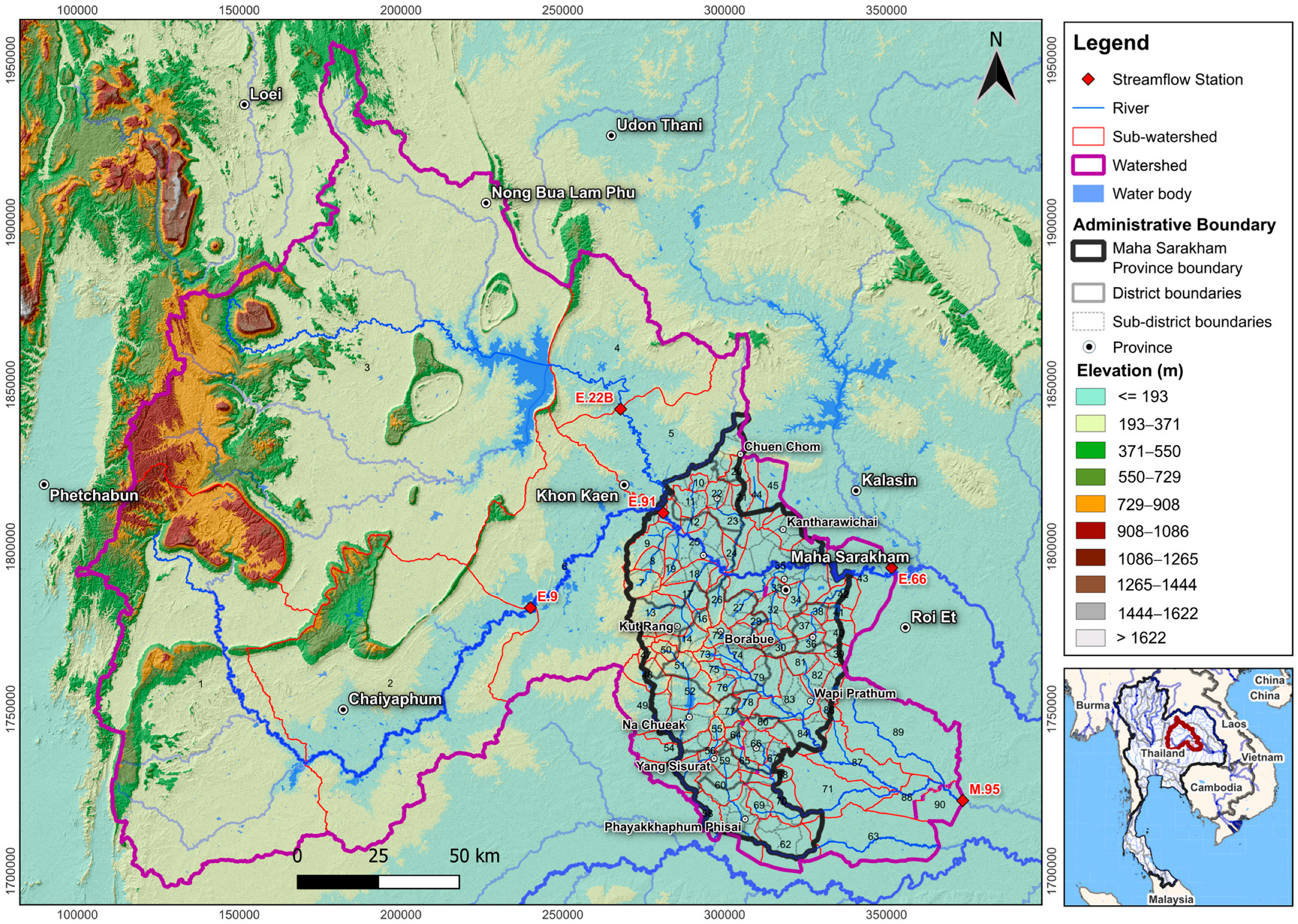
Figure 1. Topographic and hydrological features of the study area. Numbers (1–90) denote sub-watersheds delineated, covering the headwater areas in the west and refined within Maha Sarakham Province to align with sub-district boundaries. The inset map shows the entire watershed boundary (red outline) within Thailand.
Sustainability 18 01932 g001
Figure 2. Spatial distributions of meteorological monitoring stations and delineation of rainfall catchment areas using the Thiessen polygon method. Dashed lines represent Thiessen polygon boundaries for rainfall spatial interpolation.
Sustainability 18 01932 g002
Figure 3. Spatial data for the development of QSWAT HRUs: (a) land-use map and (b) soil-type map.
Sustainability 18 01932 g003
Figure 4. Spatial data used for water balance assessment in the WEAP model.
Sustainability 18 01932 g004
Figure 5. Structure and components of the WEAP model in Maha Sarakham Province.
Sustainability 18 01932 g005
Figure 6. Integrated QSWAT–WEAP system for water scarcity risk assessment: (a) System architecture showing the institutional gap between hydrological domain at watershed scale and administrative domain at sub-district scale, with the integration system serving as the bridge for scale transformation; (b) detailed framework for water balance assessment, showing specific data inputs, processing modules, and spatial analytical outputs at the sub-district level.
Sustainability 18 01932 g006
Figure 7. QSWAT and WEAP performance assessment results.
Sustainability 18 01932 g007
Figure 8. Comparison of QSWAT and WEAP simulated streamflow values with observed data (2010–2023): (a) E.9; (b) inflow of Ubolrat Dam; (c) E.22B, (d) E.91; (e) E.66A; (f) M.95.
Sustainability 18 01932 g008
Figure 9. Sub-district streamflow analysis: (a) spatial distribution by sub-district; (b) quantitative area analysis at the local level; (c) monthly temporal changes in Ranges 1–3; (d) monthly temporal changes in Ranges 4–5.
Sustainability 18 01932 g009
Figure 10. Sub-district water demand analysis: (a) Spatial distribution by sub-district; (b) quantitative area analysis at the local level; (c) monthly temporal changes in Ranges 1–5; (d) average annual water demand by sector; (e) annual quantity temporal changes.
Sustainability 18 01932 g010
Figure 11. Sub-district water shortage analysis: (a) Spatial distribution by sub-district; (b) quantitative area analysis at the local level; (c) monthly temporal changes in Range 1; (d) monthly temporal changes in Ranges 2–5.
Sustainability 18 01932 g011
Figure 12. Sub-district level of water shortage analysis: (a) spatial distribution by sub-district; (b) quantitative analysis at the local level from very low (0–5%) to very high (>45%) severity; (c) monthly temporal changes in very low level (0–5%) sub-districts; and (d) monthly temporal changes in low level (5–15%) to very high (>45%) sub-districts.
Sustainability 18 01932 g012
Table 1. Data collected as QSWAT inputs.
No.Type of DataResolutionRangeSources
1Watershed physical data
1.1Digital Elevation Model30 × 30 m2019SRTM
1.2Land-use map30 × 30 m2019LDD
1.3Soil-type map30 × 30 m2019LDD
1.4Watershed boundary, water bodies, and stream network DWR
2Meteorological data
2.1RainfallDaily2010–2023TMD, HII
2.2Maximum–minimum temperatures, relative humidity,
wind speed, and sunshine hours
Daily2010–2023TMD
3Hydrological data
3.1Streamflow at Stations E.9, E.22B, E.91, E.66A, and M.95Daily2010–2023RID
3.2Inflow of Ubolrat ReservoirDaily2010–2023EGAT
4Ubolrat Reservoir physical data
4.1Normal and maximum storage capacityMonthly2010–2023EGAT
4.2Normal and maximum surface areaMonthly2010–2023EGAT
4.3Storage targetMonthly2010–2023EGAT
4.4Maximum and minimum releaseMonthly2010–2023EGAT
Note: Bold entries denote data category headings used to organize model input types.
Table 2. Data collected as WEAP inputs.
No.Type of DataUnitSourceRemark
1Available water supply data (water resources)
1.1Streamflow data from the QSWAT modelMCM/monthQSWATUsed as available water resources for water allocation and water balance analysis in WEAP
1.2Reservoir data (reservoir capacity, storage–elevation curve, evaporation rate, reservoir operation rule)MCM/monthEGATUsed as operational constraints for reservoir simulation in WEAP
2Spatial data
2.1Rivers and water resources-DWRUsed as a spatial framework for defining river networks, demand nodes, and allocation structure in WEAP
2.2Sub-district, district, and province boundaries DOPA-
2.3Watershed boundaries-DWR-
2.4Irrigated areas within the study area-RIDIrrigated land covers 1098.2 sq.km, of which Maha Sarakham accounts for 402.6 sq.km (36.8%)
2.5Stream gauge locations-RID-
3Water demand data Used for estimating sectoral water demand at the sub-district level in WEAP
3.1Agricultural water demand (rain-fed area and irrigated area)MCM/monthOAE, LDD, RID
3.2Domestic water demandMCM/monthDOPA, PWA
3.3Industrial water demandMCM/monthDIW
3.4Service sector water demandMCM/monthDLA/NSO
Note: Bold text indicates main data categories for WEAP model input.
Table 3. The optimal parameter values obtained through calibration and validation of QSWAT.
RankParameterDescriptionFitted ValueAdjust Ranget-Statp-Value
1V__GWQMN.gwBaseflow alpha factor (days)3537.5000–50007.300.000000
2R__SOL_AWC.solAvailable water capacity of the soil layer0.07−0.4–0.45.640.000000
3V__GW_REVAP.gwGroundwater “revap” coefficient0.180.02–0.25.310.000000
4V__ALPHA_BF.gwThreshold depth of water in the shallow aquifer required for return flow to occur (mm)0.830–13.620.000381
5V__GW_DELAY.gwGroundwater delay (days)362.8530–4502.360.019295
6R__SOL_K.solSaturated hydraulic conductivity0.05−0.4–0.4−1.890.060140
7R__CN2.mgtSCS runoff curve number0.07−0.5–0.11.560.121035
8V__CH_N2.rteManning’s “n” value for the main channel0.020.01–0.1−1.480.140046
9V__CH_K2.rteEffective hydraulic conductivity in main channel alluvium26.500–200−1.170.242679
10V__REVAPMN.gwThreshold depth of water in the shallow aquifer for “revap” to occur (mm)48.7500–1000.840.399348
11V__EPCO.bsnPlant uptake compensation factor0.940–10.700.482973
12V__CH_N1.subManning’s “n” value for tributary channels0.0220.01–0.1−0.500.615715
13V__ESCO.bsnSoil evaporation compensation factor0.8680–1−0.470.639584
14R__SLSUBBSN.hruAverage slope length−0.330−0.4–0.40.070.941914
Table 4. Synthesis of water balance and shortage risk assessment by sub-district classification.
ClassificationNo. of
Sub-Districts
Area (sq.km)% of
Total Area
Streamflow Level (MCM Per Year)Demand Level (MCM Per Year)Shortage LevelRisk Level
Surplus114899High: Ranges 4–5 (250–7600)Low–Medium: Ranges 1–3 (1–30)Very Low to LowLow
Balanced1670913Medium: Range 3 (100–250)Medium: Ranges
2–3 (10–30)
MediumModerate
Deficit106409478Low: Ranges 1–2
(2–100)
Medium–High: Ranges 2–5
(10–55)
High to Very HighHigh
Total1335292100
Table 5. Characteristics of sub-districts by water shortage risk level.
Risk LevelNo. of
Sub-Districts
Area (sq.km)% of AreaDistance from Chi River (km)Streamflow
Density
(MCM Per sq.km)
Primary Water SourceCritical PeriodKey
Vulnerability
Factor
Very low2484616.0<5>100Chi RiverNoneLow vulnerability
Low41432.75–1010–100Chi River + tributariesMar–AprLimited dry season supply
Medium32139726.410–152–10TributariesFeb–MaySeasonal fluctuation
High40166431.415–250.5–2Tributaries + rainfallJan–MayDistance from main river
Very high33124223.5>25<0.5Rainfall
dependent
Nov–JunNo reliable water source
Total1335292100
Disclaimer/Publisher’s Note: The statements, opinions and data contained in all publications are solely those of the individual author(s) and contributor(s) and not of MDPI and/or the editor(s). MDPI and/or the editor(s) disclaim responsibility for any injury to people or property resulting from any ideas, methods, instructions or products referred to in the content.