Supplier Evaluation in the Electric Vehicle Industry: A Hybrid Model Integrating AHP-TOPSIS and XGBoost for Risk Prediction

Abstract

As the supply chain of the electric vehicle (EV) industry becomes increasingly complex and vulnerable, traditional supplier evaluation methods reveal inherent limitations. These approaches primarily emphasize static performance while neglecting dynamic future risks. To address this issue, this study proposes a comprehensive supplier evaluation model that integrates a hybrid Analytic Hierarchy Process (AHP) and Technique for Order Preference by Similarity to Ideal Solution (TOPSIS) framework with the Extreme Gradient Boosting (XGBoost) algorithm, contextualized for the EV sector. The hybrid AHP-TOPSIS framework is first applied to rank suppliers based on multidimensional performance criteria, including quality, delivery capability, supply stability and scale. Subsequently, the XGBoost algorithm uses historical monthly data to capture nonlinear relationships and predict future supplier risk probabilities. Finally, a risk-adjusted framework combines these two components to construct a dynamic dual-dimensional performance–risk evaluation system. A case study using real data from an automobile manufacturer demonstrates that the hybrid AHP–TOPSIS model effectively distinguishes suppliers’ historical performance, while the XGBoost model achieves high predictive accuracy under five-fold cross-validation, with an AUC of 0.851 and an F1 score of 0.928. After risk adjustment, several suppliers exhibiting high performance but elevated risk experienced significant declines in their overall rankings, thereby validating the robustness and practicality of the integrated model. This study provides a feasible theoretical framework and empirical evidence for EV enterprises to develop supplier decision-making systems that balance performance and risk, offering valuable insights for enhancing supply chain resilience and intelligence.

1. Introduction

In recent years, the global electric vehicle (EV) industry has experienced rapid growth, becoming a key driver of the automotive sector’s transformation and upgrading [1]. China’s new energy vehicle (NEV) industry holds a leading position in the global market and has established a complete industrial chain featuring coordinated development across key segments, including power batteries, electric motors, and electronic control systems. According to the Development Plan of New Energy Automobile Industry (2021–2035) issued by the General Office of the State Council, the development of NEVs is identified as an essential pathway for China to transition from a major automotive producer to a leading automotive power. The plan positions NEV development as a strategic initiative to address climate change and advance green development. It further sets the goal of enabling China, over 15 years of sustained effort, to reach internationally advanced levels in core NEV technologies and to build high-quality, globally competitive brands.

According to data from the China Association of Automobile Manufacturers (CAAM), China has ranked first globally in NEV sales for ten consecutive years. From January to September 2025, NEV production and sales reached 11.243 million and 11.228 million units, representing year-on-year increases of 35.2% and 34.9%, respectively. During the same period, NEVs accounted for 46.1% of total new vehicle sales. Driven by both policy and market forces, China’s NEV industry continues to expand, fostering rapid growth among emerging suppliers of power batteries, automotive-grade chips, and intelligent connectivity modules. However, as the industry rapidly scales up and expands its global footprint, the complexity and vulnerability of its supply chain have become increasingly pronounced [2].

The supply chain is a dynamic functional network centered on a core enterprise that integrates information, logistics, and capital flows across all stages (from raw material procurement and component manufacturing to vehicle assembly and final delivery), thereby tightly connecting upstream suppliers, manufacturers, distributors, retailers, and end users. Compared with traditional fuel vehicle supply chains, EV supply chains exhibit distinct structural characteristics. First, power batteries rely heavily on critical minerals such as lithium, cobalt, and nickel, which are concentrated in a few countries, making supply chain security highly sensitive to global resource dynamics [3]. Second, the core systems of batteries, electronic controls, and electric motors undergo frequent technological iterations, requiring the supply chain to maintain high agility and technological synchronization [4]. Third, global procurement and multimodal transportation substantially increase logistics complexity and uncertainty. Fourth, differences among countries in carbon-emission standards, charging infrastructure deployment, and fiscal incentive policies require greater adaptability and regional optimization within the supply chain [2].

Against this backdrop, China’s NEV industry faces three major categories of risk:

• Critical raw material supply disruptions: The heavy reliance of core components such as power batteries on rare earth and nonferrous metals makes upstream supply vulnerable to international market volatility and geopolitical tensions, potentially causing production interruptions.
• Geopolitical and policy uncertainties: As domestic automakers accelerate their overseas expansion, trade barriers, tariff adjustments, and regional political events increasingly amplify the external vulnerabilities of supply chains [5].
• Technological iteration and market volatility: In the era of the Software-Defined Vehicle (SDV), supply chain challenges such as automotive-grade chip shortages, hardware–software integration issues, and rapidly shifting consumer preferences have emerged as new systemic risks.

These structural characteristics imply that supplier performance in the EV industry cannot be adequately assessed by traditional static evaluation frameworks alone. In particular, rapid technological iteration requires suppliers not only to meet current quality standards, but also to maintain stable production processes and fast response capabilities under frequent design changes. Meanwhile, raw material scarcity and supply concentration amplify the importance of delivery resilience and capacity stability, which are often underrepresented in conventional supplier evaluation models.

The Decision of the Central Committee of the Communist Party of China on Further Enhancing the Resilience and Security of Industrial and Supply Chains explicitly advocates for establishing an industrial system that is efficient, secure, and controllable. Similarly, the Opinions of the General Office of the CPC Central Committee and the General Office of the State Council on Accelerating the Development of a Unified and Open Transportation Market emphasize strengthening resilience and security in logistics supply chains. These policies provide top-level guidance for strengthening the resilience and risk management of New Energy Vehicle (NEV) supply chains. Consequently, supply chain management in China’s NEV enterprises is shifting from a traditional cost-oriented approach to a strategic management paradigm that emphasizes risk prediction, rapid response, and ecosystem resilience [6,7].

Therefore, establishing a scientific system for supplier evaluation and risk prediction constitutes a crucial prerequisite for ensuring the safe and stable operation of the EV industry chain. Unlike traditional supplier evaluation models that focus primarily on static cost or quality performance, the proposed research context emphasizes process stability, delivery resilience, and capacity assurance, which are particularly critical under the EV industry’s rapid technological iteration and increasing dependence on scarce raw materials [8,9].

Although emerging machine learning approaches are capable of predicting potential supply risks with high accuracy, their interpretability is often confined to model-level or feature-level explanations (e.g., SHAP-based attribution) and does not necessarily align with the structured evaluation logic required for managerial decision-making [10]. In practice, decision-makers in complex supply chains require an explicit and hierarchical assessment framework to understand the relative importance of quality, delivery reliability, and supply stability prior to risk prediction.

Against this background, this study integrates multi-criteria decision-making (MCDM) methods with machine learning techniques within the specific context of the EV supply chain, developing an AHP–TOPSIS–XGBoost framework that combines structured, interpretable performance evaluation with data-driven supplier risk prediction. By capturing the temporal evolution of supplier risk while preserving transparent evaluation logic, the proposed approach explicitly addresses EV-specific challenges such as rapid technological iteration and raw material supply constraints, thereby supporting robust supplier screening and dynamic risk monitoring in EV supplier management.

The remainder of this paper is organized as follows: Section 2 presents an in-depth literature review of supplier evaluation, MCDM, and supply chain risk prediction, establishing the theoretical foundation and identifying the research gap. Section 3 introduces the integrated AHP–TOPSIS–XGBoost model for supplier evaluation and risk prediction. Section 4 presents empirical validation of the model’s effectiveness. Section 5 reports the case study results and demonstrates the practical effectiveness of the proposed model. Section 6 discusses the theoretical implications, limitations, and future research directions.

2. Literature Review on Supplier Evaluation and Risk Prediction

The selection and evaluation of suppliers directly affect a company’s cost control, production efficiency, and product quality [11]. As market competition intensifies, supplier evaluation has gradually become a crucial component of corporate strategic management. Scholars worldwide have examined this topic from diverse perspectives, developing a comprehensive evaluation framework centered on Multi-Criteria Decision Making (MCDM). Building on this foundation, the introduction of machine learning and intelligent algorithms has propelled supply chain risk prediction into the data-driven era.

Early studies primarily adopted qualitative approaches such as the Delphi method, expert scoring, and fuzzy set theory. These methods feature clear structures and straightforward implementation but rely heavily on expert judgment, introducing strong subjectivity. Amiri et al. [12] proposed a fuzzy set-based supplier selection model that addresses the limitations of traditional evaluations by incorporating uncertainty criteria. Subsequently, quantitative models were introduced to reduce subjectivity. Common methods include the Analytic Hierarchy Process (AHP), Data Envelopment Analysis (DEA), and the Technique for Order Preference by Similarity to Ideal Solution (TOPSIS). AHP determines weights through hierarchical structures and pairwise comparison matrices, offering logical clarity and suitability for complex criteria systems. DEA measures relative efficiency using input–output models, while TOPSIS ranks alternatives based on their distance from an ideal solution. These quantitative methods enable multi-criteria assessment with high stability and comparability. Goodarzi et al. [13] demonstrated that integrating multi-criteria decision-making with multi-objective optimization effectively reduces the subjectivity inherent in expert-based assessments, providing a more objective and robust foundation for supplier evaluation. Dos Santos et al. [14] applied an entropy-weighted TOPSIS model to assess green suppliers, confirming the method’s strong stability, comparability, and effectiveness in multi-criteria decision environments. Deretarla et al. [15] applied AHP to derive criterion weights in a multi-level supplier evaluation framework, demonstrating its effectiveness in handling complex criteria with clear and objective logic. Marzouk and Sabbah [16] proposed an AHP–TOPSIS framework for socially sustainable supplier selection in construction supply chains.

Meanwhile, the application of DEA in supplier performance evaluation has continued to deepen. Dutta et al. [17] conducted a systematic review of DEA applications in supplier selection from 2000 to 2020, concluding that DEA effectively handles multi-input and multi-output problems. Vörösmarty and Dobos [18] developed a DEA-based framework for sustainable performance evaluation that integrates economic, environmental, and social dimensions. Samavati et al. [19] proposed a dynamic network DEA model that evaluates sustainable supply chain performance across multiple periods while accounting for undesirable outputs, providing a more comprehensive view of time-varying efficiency. Overall, supplier evaluation methods have evolved from qualitative judgment to quantitative modeling and from static assessment to dynamic optimization, with a clear trend toward intelligence methods and integration.

In recent years, the rapid development of big data and artificial intelligence has led to the widespread application of machine learning (ML) methods in supplier evaluation and supply chain risk prediction. ML can uncover complex nonlinear relationships from historical operational data, enabling highly accurate predictions of supplier performance, delivery stability, and disruption risk. Among various algorithms, tree-based models have become particularly valuable tools for supplier data analysis due to their interpretability and strong generalization capability. Jahin et al. [20] emphasized that tree models (e.g., Random Forest, XGBoost) outperform traditional statistical methods in both interpretability and stability for risk identification and performance prediction. Similarly, Ali et al. [21] utilized the Random Forest algorithm to develop a decision support system for classifying supplier selection criteria. Sani et al. [22] developed a Bayesian-optimized LightGBM model for back-order risk prediction in supply chains, illustrating the strong predictive capacity of tree-based ML models under uncertain supply chain conditions. De Backker et al. [23] applied the XGBoost model to predict disruption risks for critical components for automotive OEMs. They developed a component risk matrix to quantify risk exposure across parts, providing a practical pathway to enhance supply chain resilience. These studies collectively demonstrate that ML significantly improves enterprises’ ability to identify and respond to potential supply chain risks.

To overcome the static limitations of traditional MCDM approaches and the interpretability deficiencies of pure ML models, hybrid models combining the strengths of both have become a prominent research focus. Gidiagba et al. [24] proposed a hybrid model integrating Non-negative Matrix Factorization (NMF), Random Forest, and TOPSIS for supplier evaluation in the pharmaceutical industry, achieving a unified framework for dimensionality reduction, weight learning, and comprehensive ranking. Similarly, Ishizaka et al. [25] introduced the BWM–GAIA model in a closed-loop pharmaceutical supply chain, integrating optimization algorithms with hierarchical weighting methods to enable sustainable supplier selection. Galdo et al. [26] combined MCDM with Artificial Neural Networks (ANN) to optimize internal combustion engine emission performance, further validating the cross-domain applicability of MCDM–ML integration.

In summary, current research is shifting from single-algorithm approaches toward integrated, interpretable frameworks. Hybrid models combine the expert-driven decision logic of MCDM with the data-driven learning capability of ML, providing a new methodological foundation for comprehensive supplier evaluation. However, existing studies still exhibit limitations in the manufacturing sector, particularly within the EV industry chain. On the one hand, most models emphasize static performance rankings and fail to reflect dynamic variations in supply risk. On the other hand, although ML models exhibit strong predictive performance, they often lack systematic weight interpretation and decision-support mechanisms. Therefore, developing a hybrid framework that leverages MCDM for performance ranking while integrating ML for dynamic risk prediction represents an urgent and critical challenge in EV supply chain management research.

3. Multi-Dimensional Supplier Evaluation Model Based on Historical Data

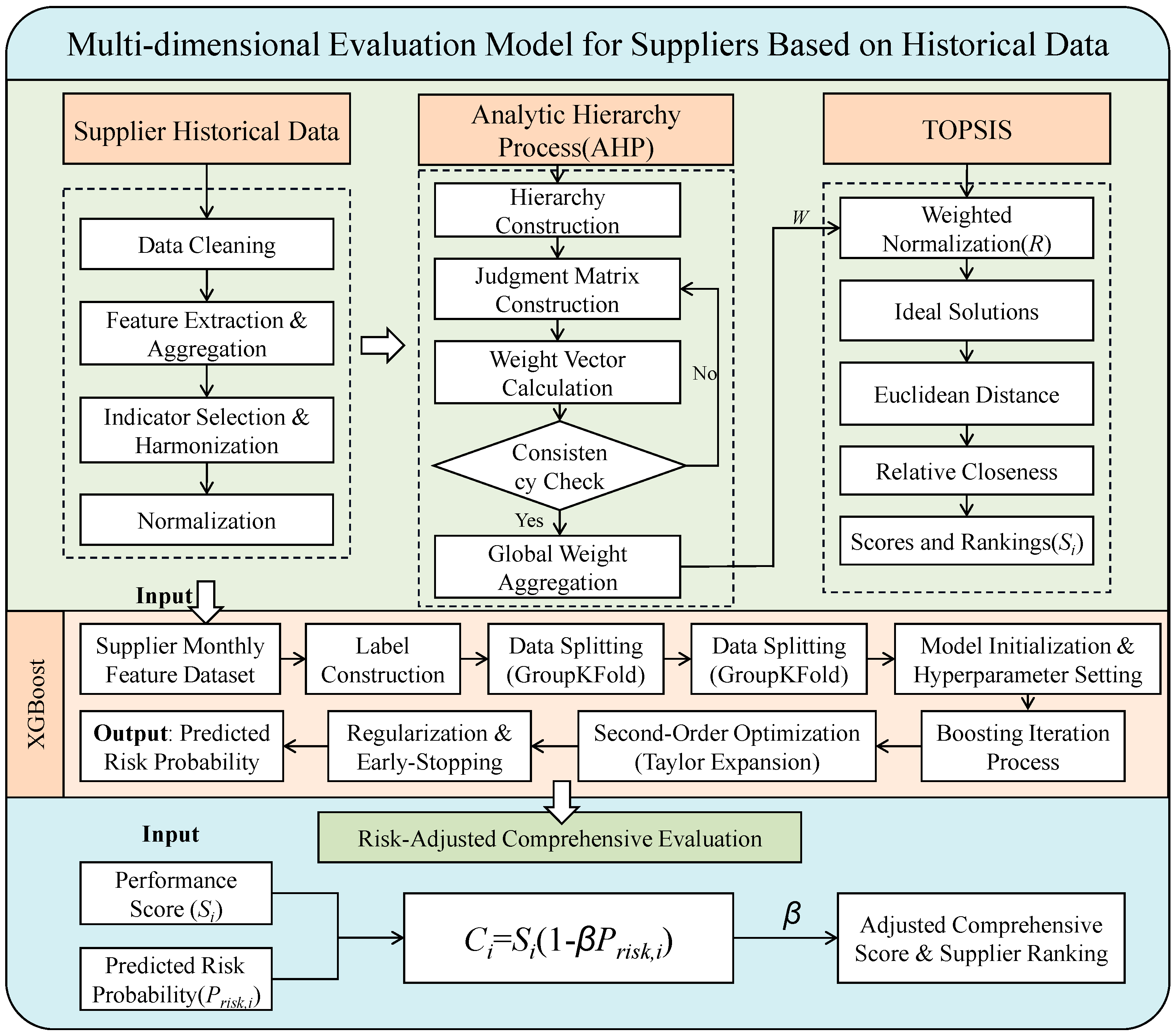
This study aims to overcome two primary challenges in supplier evaluation: the static limitations of traditional Multi-Criteria Decision-Making (MCDM) methodologies, which emphasize historical performance while neglecting dynamic risks, and the interpretability challenges inherent in machine learning (ML) models for risk prediction. To address these issues, a comprehensive supplier evaluation model is developed by integrating the AHP–TOPSIS method with the XGBoost algorithm. This integrated approach leverages the respective strengths of each technique: the Analytic Hierarchy Process (AHP) for determining criteria weights, the Technique for Order Preference by Similarity to Ideal Solution (TOPSIS) for multi-criteria comprehensive evaluation, and the Extreme Gradient Boosting (XGBoost) algorithm for dynamic risk prediction. Collectively, they constitute a unified technical framework comprising four modules: multidimensional profiling modeling, hierarchical weight determination, multi-criteria comprehensive evaluation, and risk-adjusted prediction. The overall architecture of the proposed model is presented in Figure 1.

This framework preserves the interpretability and decision transparency of the traditional AHP-TOPSIS model while incorporating the dynamic predictive capability of machine learning. In doing so, it achieves an integrated analytical framework that unifies supplier evaluation and risk prediction.

3.1. Determination of the AHP Criteria System and Weights

3.1.1. Construction of the Supplier Evaluation Criteria System

In complex supply chain systems, supplier performance is jointly influenced by multiple interrelated factors, including product quality, delivery reliability, process stability, and capacity allocation. In the context of electric vehicle (EV) manufacturing, these factors are further shaped by rapid technological iteration, stringent quality requirements for core components, and increasing supply uncertainty caused by material constraints and logistics disruptions. Therefore, establishing a structured and operable supplier evaluation framework is a prerequisite for effective performance assessment and risk analysis.

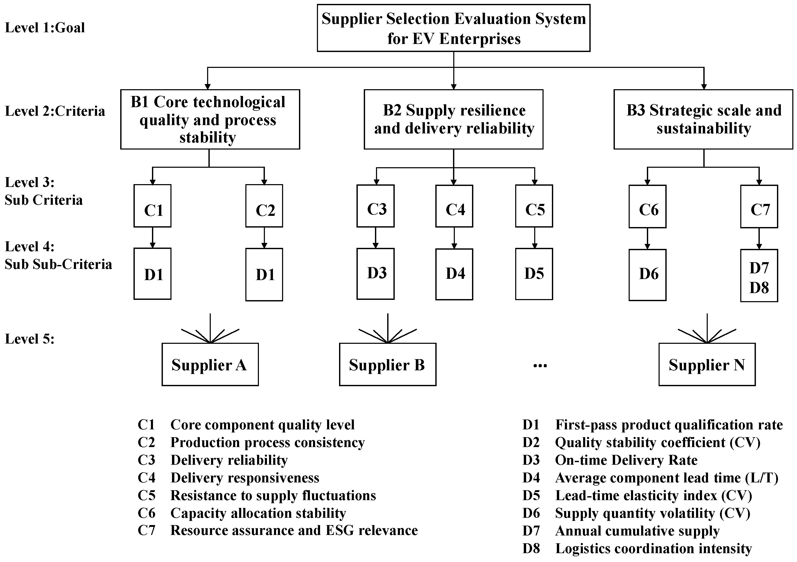
To this end, this study constructs a hierarchical supplier evaluation criteria system based on the Analytic Hierarchy Process (AHP). Considering the operational characteristics of the EV supply chain, three primary dimensions are defined: core technological quality and process stability, supply resilience and delivery reliability, and strategic scale and sustainability.

The proposed evaluation framework follows a three-tier hierarchical structure. The objective layer (A-layer) represents the comprehensive performance of core EV suppliers. The first-level criteria (B-layer) capture the three primary dimensions described above. The second-level criteria (C-layer) further decompose each dimension into key operational aspects, while the third-level criteria (D-layer) consist of specific and quantifiable indicators derived from suppliers’ operational data. This hierarchical structure enables a systematic representation of supplier performance attributes and provides a consistent basis for subsequent weight determination and multi-criteria evaluation.

The complete hierarchical criteria system is illustrated in Figure 2. To ensure a rigorous understanding of the multi-dimensional framework,

Table 1. Definitions of evaluation indicators.

Criteria	Definition and Contextual Relevance in EV Industry
D1 First-pass product qualification rate	The average qualification rate across all batches; reflects the technical reliability of critical EV components (e.g., IGBTs, motors)
D2 Quality stability coefficient (CV)	The coefficient of variation of the qualification rate; evaluates the process control consistency of automated EV production lines.
D3 On-time Delivery Rate	The proportion of orders delivered within the schedule; essential for maintaining the agility of EV Just-In-Time (JIT) assembly.
D4 Average component lead time (L/T)	The mean time interval from order to arrival; represents the supply chain’s responsiveness to rapid EV technological iterations.
D5 Lead-time elasticity index (CV)	The coefficient of variation of lead times; measures the supplier’s resilience against logistical shocks or material shortages.
D6 Supply quantity volatility (CV)	The coefficient of variation of delivered quantities; indicates the stability of capacity allocation during fluctuating demand periods.
D7 Annual cumulative supply scale	The total volume of components supplied; reflects the strategic capability to secure critical resources such as battery minerals.
D8 Logistics coordination	The frequency or proportion of order interactions; serves as a proxy for operational synergy and governance coordination.

provides the definitions and contextual relevance of the selected indicators within the electric vehicle (EV) supply chain environment.

3.1.2. Determination of Evaluation Criteria Weights

After establishing the comprehensive supplier evaluation system, this study employs the Analytic Hierarchy Process (AHP) to determine the weights of the evaluation criteria, thereby ensuring a scientifically grounded and reasonable allocation of their importance in the overall assessment. AHP is a multi-criteria decision-making method that decomposes complex problems into a hierarchical structure and quantifies the relative importance of factors. Pairwise comparison matrices are constructed from expert judgments, and the relative weights of criteria at each level are calculated using the eigenvalue or geometric mean (square root) method, thereby capturing each criterion’s contribution to the overall objective [27].

The AHP-based weight determination process mainly consists of three steps: constructing the pairwise comparison matrix; (2) calculating the eigenvector and deriving the weights; (3) performing a consistency check.

• Constructing the pairwise comparison matrix

Based on the three-level criteria system established in the previous subsection, and taking comprehensive supplier performance evaluation as the overall objective level, pairwise comparisons are conducted among the primary criteria (B1–B3) to construct the judgment matrix $A={[a_{ij}]}_{n\times n}$. Each matrix element $a_{ij}$ represents the relative importance of criterion i compared with criterion j. The pairwise comparisons adopt the 1–9 scale proposed by Saaty [27], where 1 signifies equal importance, 3 slight importance, 5 clear importance, 7 strong importance, and 9 extreme importance, with 2, 4, 6, and 8 as intermediate values. If criterion i is more important than criterion j, then $a_{ij}>1$; conversely, if criterion j is more important than criterion i, then $a_{ij}<1$; when the two criteria are equally important, $a_{ij}=1$.

Based on the comprehensive judgment results of the expert panel, the judgment matrix from the criterion level (Level B) to the objective level (Level A), as well as the judgment matrices from each secondary criterion (Level C) and tertiary criterion (Level D) to their corresponding superior criteria, are obtained. All matrices satisfy the principles of reciprocity and positive consistency, expressed as follows:

$$a_{ij}>0,a_{ji}={\displaystyle \frac{1}{a_{ij}}},a_{ii}=1$$

(1)

• Weight Calculation

After obtaining the judgment matrices, the weights of each criterion relative to its superior objective must be calculated. In this study, the eigenvalue method is employed to derive the weight vector by calculating the maximum eigenvalue of the judgment matrix and its corresponding eigenvector, which reflects the relative importance of each criterion. The calculation steps are as follows:

• Calculate the geometric mean of each row in the judgment matrix:

  $$M_i={\left({\displaystyle \prod _{j=1}^n{a}_{ij}}\right)}^{1/n}$$

  (2)
• Normalize to obtain the weight vector:

  $$W_i={\displaystyle \frac{M_i}{{\displaystyle \sum _{i=1}^n{M}_i}}},i=1,2,\dots ,n$$

  (3)

  where $W_i$ represents the weight of the i-th criterion relative to the superior objective, and the weights satisfy the normalization condition ${\displaystyle \sum _{i=1}^n{W}_i}=1$.
• Calculate the maximum eigenvalue of the judgment matrix:

  $${\lambda }_{\max }={\displaystyle \sum _{i=1}^n\frac{{(AW)}_i}{n{W}_i}}$$

  (4)

  where A denotes the judgment matrix, and ${(AW)}_i$ is the i-th element of the matrix product $AW$.

By sequentially calculating the weights for the criterion and indicator levels, the local weights of each hierarchy are obtained. Multiplying the weights layer by layer yields the comprehensive weight of each bottom-level indicator (Level D). This comprehensive weight reflects each indicator’s final contribution to the overall evaluation objective and serves as an input parameter for subsequent weighted calculations in the TOPSIS model.

• Consistency Check

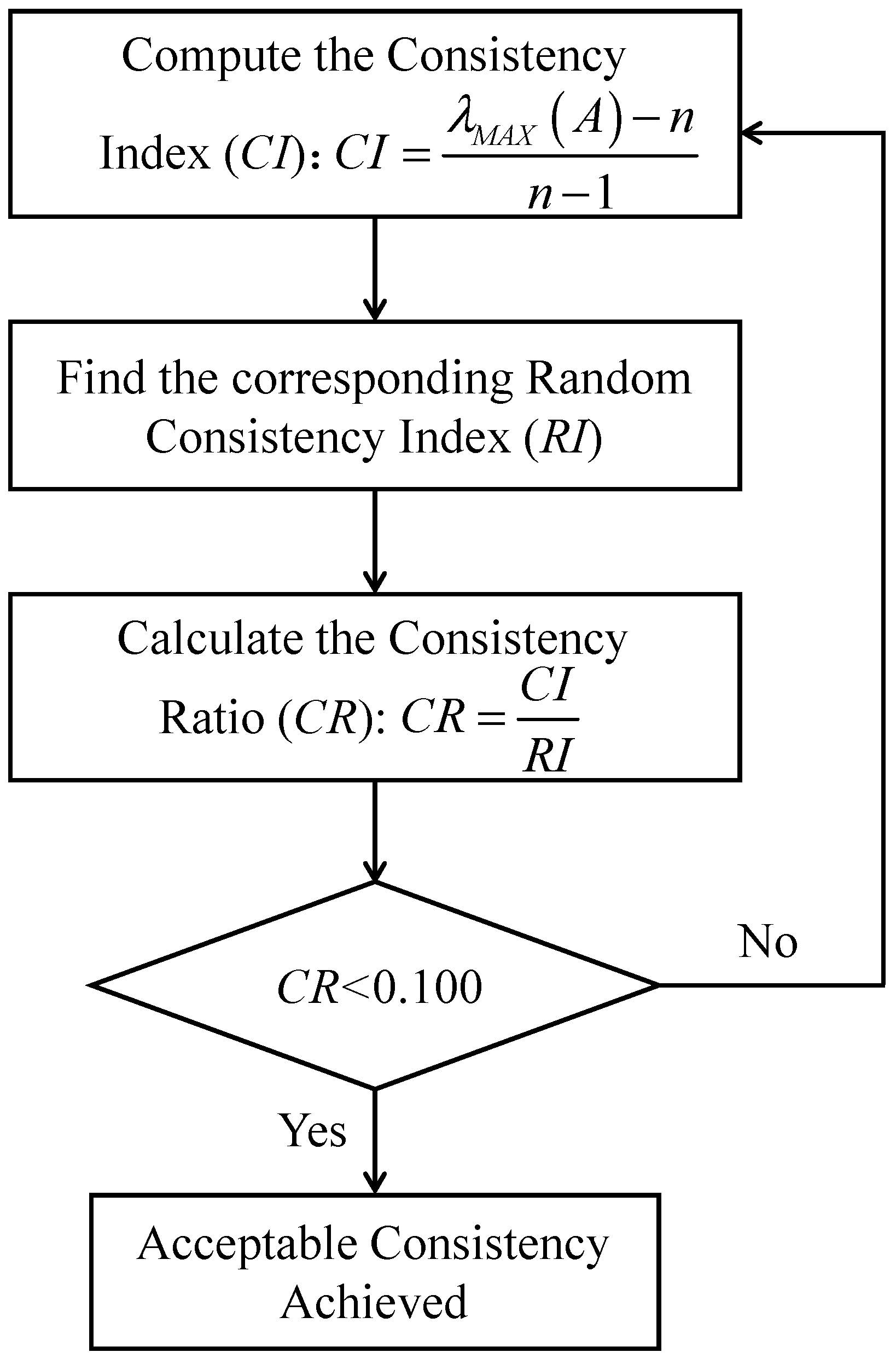
Since the judgment matrices are derived from expert subjective judgments, a consistency check is required to ensure the reliability of the results. The Analytic Hierarchy Process (AHP) uses the Consistency Index (CI) and Consistency Ratio (CR) as verification measures, calculated as follows:

$$CI={\displaystyle \frac{{\lambda }_{\max }-n}{n-1}},CR={\displaystyle \frac{CI}{RI}}$$

(5)

where RI is the average random consistency index, and its value depends on the order n of the matrix. For typical matrix orders, RI takes the values 0.58 (n = 3), 0.90 (n = 4), 1.12 (n = 5), 1.24 (n = 6), 1.32 (n = 7), 1.41 (n = 8), and 1.45 (n = 9). When CR < 0.10, the judgment matrix is considered to have satisfactory consistency, and the calculated weights are deemed reliable. When CR ≥ 0.10, the judgment matrix must be revised until the consistency condition is satisfied.

The consistency check procedure is illustrated in Figure 3.

3.2. TOPSIS Comprehensive Evaluation Model

After determining the weights of each evaluation criterion, the Technique for Order Preference by Similarity to Ideal Solution (TOPSIS) is introduced to construct a comprehensive evaluation model for quantitatively ranking suppliers. This method, a classic multi-criteria decision analysis (MCDA) technique, evaluates alternatives by calculating their relative closeness to the ideal solution, thereby deriving an overall ranking of performance [28]. Compared with other multi-attribute decision-making methods, TOPSIS accommodates both benefit-oriented and cost-oriented criteria while preserving indicator weight differentiation. It offers advantages such as computational simplicity, intuitive interpretation, and high stability.

In this study, an improved TOPSIS model is employed to rank suppliers’ comprehensive performance. The fundamental principle is to calculate each supplier’s distance to both the Positive Ideal Solution (PIS) and the Negative Ideal Solution (NIS) within a normalized and weighted criteria space, then determine rankings based on their relative closeness. The algorithm proceeds as follows:

• Constructing the Standardized Decision Matrix

Suppose there are m evaluation objects (suppliers) and n evaluation criteria. Let the set of alternatives be denoted as $M=\left(M_1,M_2,\dots ,M_m\right)$ and the set of criteria as $C=\left(C_1,C_2,\dots ,C_n\right)$. The value of an alternative $M_i$ with respect to a criterion $C_j$ is denoted as $z_{ij}$, forming a multi-criteria decision matrix $Z={\left(z_{ij}\right)}_{m\times n}$. As different criteria may possess distinct units of measurement, normalization of the original data is necessary to ensure comparability.

For benefit-oriented (positive) criteria, apply the following extreme-value normalization formula:

$${x^{\prime }}_{ij}={\displaystyle \frac{x_{ij}-x_j^{mn}}{x_j^{\max }-x_j^{\min }}}$$

(6)

For cost-oriented (negative) criteria, apply the inverse normalization formula:

$${x^{\prime }}_{ij}={\displaystyle \frac{x_j^{\max }-x_{ij}}{x_j^{\max }-x_j^{\min }}}$$

(7)

After normalization, the standardized decision matrix is obtained as $V={\left(v_{ij}\right)}_{m\times n}$.

• Weighted Standardized Matrix

To account for the relative importance of each criterion, the standardized matrix is weighted using the AHP-derived weight vector W. The weighted standardized decision matrix is then computed as:

$$R={[r_{ij}]}_{m\times n},r_{ij}=W_j\times z_{ij}$$

(8)

This matrix reflects both the relative performance of each indicator and the distribution of weights, serving as the basis for the subsequent distance calculations.

• Determining the Positive Ideal and Negative-Ideal Solutions

Within the weighted standardized space, define the Positive Ideal Solution (PIS) and Negative Ideal Solution (NIS) as follows

$$c_j^{*}=\max c_{ij}(j=1,2,\dots ,n)$$

(9)

$$c_j^0={\min }_i{c}_{ij}(j=1,2,\dots ,n)$$

(10)

• Calculating the Distance to Ideal Solutions

The Euclidean distance is used to calculate each supplier’s distance to the PIS and NIS:

$$D_i^{+}=\sqrt{{\displaystyle \sum _{j=1}^n{(r_{ij}-r_j^{+})}^2}}$$

(11)

$$D_i^{-}=\sqrt{{\displaystyle \sum _{j=1}^n{(r_{ij}-r_j^{-})}^2}}$$

(12)

where $D_i^{+}$ denotes the distance of the i-th supplier from the PIS, and $D_i^{-}$ denotes the distance from the NIS.

A smaller $D_i^{+}$ and larger $D_i^{-}$ indicate that the supplier’s performance is closer to the ideal state.

• Calculating the Relative Closeness

To comprehensively measure each supplier’s proximity to the ideal solution, define the relative closeness $S_i$ as:

$$S_i={\displaystyle \frac{D_i^{-}}{D_i^{+}+D_i^{-}}}$$

(13)

The closer $S_i$ is to 1, the better the overall performance of the supplier. Finally, suppliers are ranked according to the descending order of $S_i$ values, yielding the final comprehensive evaluation results.

3.3. XGBoost Supplier Risk Prediction Model

Building upon the comprehensive performance scores determined by the AHP–TOPSIS model, this study employs the eXtreme Gradient Boosting (XGBoost) algorithm to construct a supplier risk prediction model. This model aims to further identify potential risks and quantify the probability of future defaults or supply instability. The integration of this machine learning technique with traditional multi-criteria decision-making methods enables a quantitative assessment of potential supplier risks, grounded in a comprehensive consideration of historical performance. Consequently, this integrated framework enables a dynamic assessment of supply chain stability and sustainability.

3.3.1. Model Principles

XGBoost, introduced by Chen and Guestrin (2016), is a highly efficient implementation of the Gradient Boosted Decision Tree (GBDT) algorithm [29]. While traditional GBDT methods rely solely on first-order derivatives, XGBoost distinguishes itself by performing a second-order Taylor expansion of the loss function and incorporating a regularization term into the objective. This formulation seeks an optimal solution by balancing the reduction in the loss function with model complexity, thereby mitigating overfitting and enhancing computational efficiency. Suppose the training dataset is defined as follows:

$$D=\left\{\left(x_i,y_i\right)\mid i=1,2,\dots ,n\right\},x_i\in {ℝ}^m,y_i\in \left\{0,1\right\}$$

(14)

here, $x_i$ denotes the feature vector of the i-th data point, and $y_i$ represents the corresponding risk label, where 1 indicates the presence of risk and 0 indicates its absence. Given k regression trees (k = 1, 2,…,K), with $f_k$ representing an individual regression tree and $\mathcal{F}$ denoting the set space of all such trees, the model’s prediction function ${\widehat{y}}_i$ for an instance $x_i$ is defined as the sum of k trees:

$${\widehat{y}}_i={\displaystyle \sum _{k=1}^K{f}_k}(x_i),f_k\in \mathcal{F}$$

(15)

The optimization objective of XGBoost comprises two components: the loss function L(θ) and the regularization term Ω(θ). The complete objective function is given by:

$$Obj(\theta )=L(\theta )+\Omega (\theta )$$

(16)

This can be expanded into the following summation form over multiple iterations:

$$\mathrm{Obj}={\displaystyle \sum _{i=1}^{n}l}(y_i,{\widehat{y}}_i)+{\displaystyle \sum _{k=1}^K\Omega }(f_k)$$

(17)

In this formulation, ${\widehat{y}}_i$ is the predicted value, $y_i$ is the true value, and $l(y_i,{\widehat{y}}_i)$ denotes the loss function that quantifies the discrepancy between the prediction and the ground truth. The goal of XGBoost is to minimize the cumulative loss ${\displaystyle \sum _{i=1}^{n}l}(y_i,{\widehat{y}}_i)$. The regularization term $\Omega (f_k)$ controls the complexity of each tree and is defined as:

$$\Omega (f_k)=\gamma T+{\displaystyle \frac{1}{2}}\lambda {\displaystyle \sum _{j=1}^T{w}_j^2}$$

(18)

here, $\gamma$ is the penalty coefficient for the number of leaf nodes, T denotes the total number of leaf nodes in a tree, and $\gamma T$ constitutes the corresponding penalty term. Similarly, $\lambda$ is the penalty coefficient applied to leaf node weights, $w_j^2$ represents the weight of the j-th leaf node, and the term ${\displaystyle \frac{1}{2}}\lambda {\displaystyle \sum _{j=1}^T{w}_j^2}$ serves as the penalty on these weights. This regularization mechanism effectively suppresses the growth of excessively deep tree structures and prevents overly large leaf node weights, thereby enhancing the model’s robustness and generalization capability.

XGBoost uses a gradient boosting strategy, adding a new regression tree at each iteration. Let ${\widehat{y}}_i\left(t\right)$ denote the predicted value for the i-th sample at the t-th iteration, and $f_t(x_i)$ represent the new regression tree introduced in that iteration. The iterative process can be derived as follows:

$$\begin{array}{l}\begin{array}{l}{\widehat{y}}_i=0\\ {\widehat{y}}_i^{(1)}=f_1(x_i)={\widehat{y}}_i^{(0)}+f_1(x_i)\end{array}\hfill \\ {\widehat{y}}_i^{(2)}=f_1(x_i)+f_2(x_i)={\widehat{y}}_i^{(1)}+f_2(x_i)\hfill \\ ⋮\hfill \\ {\widehat{y}}_i^{(t)}={\displaystyle \sum _{k=1}^t{f}_k}(x_i)={\widehat{y}}_i^{(t-1)}+f_t(x_i)\hfill \end{array}$$

(19)

To facilitate optimization, XGBoost approximates the loss function using a second-order Taylor expansion:

$$l(y_i,{\widehat{y}}_i^{(t)})\approx l(y_i,{\widehat{y}}_i^{(t-1)})+g_i{f}_t(x_i)+{\displaystyle \frac{1}{2}}{h}_i{f}_t^2(x_i)$$

(20)

where $g_i$ and $h_i$ are the first-order and second-order derivatives of the loss function with respect to the predicted value, respectively:

$$\begin{array}{l}{g}_i={\displaystyle \frac{\partial l(y_i,{\widehat{y}}_i^{(t-1)})}{\partial {\widehat{y}}_i^{(t-1)}}},\\ h_i={\displaystyle \frac{{\partial }^{2}l(y_i,{\widehat{y}}_i^{(t-1)})}{\partial {({\widehat{y}}_i^{(t-1)})}^2}}\end{array}$$

(21)

Substituting Equation (21) into Equation (17) and including the regularization term yields the approximate objective function for the t-th iteration:

$$Ob{j}^{(t)}\approx {\displaystyle \sum _{i=1}^n\left[g_i{f}_t(x_i)+\frac{1}{2}{h}_i{f}_t^2(x_i)\right]}+\Omega (f_t)$$

(22)

By taking the partial derivative of Equation (22) with respect to $f_t(x_i)$ and setting it to zero, the optimal weight for each leaf node is obtained:

$$w_j^{*}=-{\displaystyle \frac{G_j}{H_j+\lambda }}$$

(23)

where $G_j={\displaystyle {\sum }_{i\in I_j}{g}_i}$ and $H_j={\displaystyle {\sum }_{i\in I_j}{h}_i}$ with $I_j$ denoting the set of samples in the j-th leaf node.

Substituting the optimal weight back into the objective function gives the optimal objective value corresponding to the tree structure:

$$Ob{j}^{(t)}=-{\displaystyle \frac{1}{2}}{\displaystyle \sum _{j=1}^T\frac{G_j^2}{H_j+\lambda }}+\gamma T$$

(24)

During each iteration, the model constructs an optimal tree structure by minimizing this objective function. The final prediction model is the ensemble of all trees, as defined in Equation (15), where $f_k(x_i)$ denotes the output of the k-th tree and the weighted sum of all trees produces the final risk prediction. For the supplier risk identification task, the predicted value ${\widehat{y}}_i$ corresponds to the probability $P_{risk,i}$ of a supplier experiencing a future risk event.

3.3.2. Risk-Adjusted Evaluation Framework

After obtaining the supplier risk probabilities from the XGBoost model, this study proposes a risk-adjusted evaluation framework. This framework integrates performance assessment with risk prediction, based on the AHP–TOPSIS comprehensive evaluation model. The framework is designed to integrate the dynamic risk predictions generated by the XGBoost model with the static performance evaluations derived from the AHP–TOPSIS model. By implementing a risk adjustment mechanism, it recalibrates the suppliers’ comprehensive scores, thereby establishing an integrated evaluation system that considers both historical performance and risk exposure. In contrast to conventional static evaluation approaches, this framework incorporates potential future risks, facilitating a transition from static decision-making to dynamic, risk-informed decision-making.

Through hierarchical weight analysis and proximity calculations, the AHP–TOPSIS model provides an objective representation of suppliers’ historical performance across dimensions such as quality, delivery, and supply stability. Nevertheless, this static evaluation framework fails to capture the dynamic evolution of future supplier risks, potentially leading to the misclassification of certain high-performance yet high-risk suppliers as preferable options. To address this limitation, the present study integrates the risk probability predictions from the XGBoost model into the comprehensive evaluation system. This adjustment of performance scores for risk enhances the model’s predictive capability and robustness.

Within the risk-adjusted evaluation framework, the comprehensive proximity degree $S_i$ for each supplier is first computed using the AHP–TOPSIS method, reflecting the supplier’s relative performance level across multiple dimensions. This score is subsequently adjusted for risk using the risk probability $P_{risk,i}$ predicted by the XGBoost model, yielding a risk-adjusted composite score $C_i$. The corresponding formula is given by:

$$C_i=S_i\times (1-\beta P_{risk,i})$$

(25)

here, $C_i$ denotes the risk-adjusted composite score; $S_i$ represents the comprehensive proximity degree calculated by AHP–TOPSIS; $P_{risk,i}$ indicates the future risk probability of the supplier predicted by the XGBoost model and $\beta$ is the risk weighting coefficient that controls the degree of adjustment applied to the composite score based on risk exposure. Depending on the enterprise’s risk appetite and management strategy, the value of $\beta$ can be flexibly set within the interval [0, 1]. When $\beta =0$, the model reduces to the traditional TOPSIS evaluation. When $\beta >0$, a larger value of $\beta$ reflects a more conservative or risk-averse decision-making posture, applying a greater penalty to high-risk suppliers.

4. Case Analysis

4.1. Data Sources and Preprocessing

Following the construction of the comprehensive evaluation framework, this study utilizes real supply chain data from an automotive manufacturing enterprise to validate the model’s effectiveness and applicability. The dataset encompasses multidimensional information from various component suppliers, covering quality, delivery, production capacity, and order fulfillment, thereby providing a holistic representation of supplier operational performance and risk profiles.

For data selection, supplier samples were filtered and characterized based on the enterprise’s monthly supply records from the past year. The resulting dataset comprises key performance indicators (KPIs) from 14 suppliers. To ensure statistical reliability, suppliers with two or fewer supply records were excluded, thereby reducing data noise and enhancing the model’s generalization. Furthermore, systematic data preprocessing was implemented to ensure scientific rigor and analytical accuracy.

Initial processing involved identifying and treating missing values and outliers in the raw data. Missing values in quality and delivery metrics were imputed using the mean. At the same time, extreme outliers were either corrected or smoothed using a combination of business expertise and the interquartile range (IQR) method to minimize statistical bias. Subsequently, min–max normalization was applied to standardize metrics with divergent units, enabling consistent cross-comparison. The normalization formula is expressed as:

$${x^{\prime }}_{ij}={\displaystyle \frac{x_{ij}-\min (x_j)}{\max (x_j)-\min (x_j)}}$$

(26)

where $x_{ij}$ denotes the original value of the j-th indicator for the i-th supplier, ${x^{\prime }}_{ij}$ represents the normalized value, and $\max (x_j)$ and $\min (x_j)$ are the maximum and minimum values of the j-th metric, respectively. This process confines all normalized data to the interval [0, 1], effectively eliminating scale and unit discrepancies among indicators and their potential influence on subsequent evaluation steps.

4.2. Determination of Supplier Evaluation Criteria Weights

Based on the three-level criteria system established in the preceding section, with comprehensive supplier performance evaluation as the objective layer, this study convened an expert panel in procurement, quality, and management, all possessing over five years of experience in the new energy vehicle supply chain, to ensure reliability and consistency of their judgments. Through multiple rounds of independent scoring and iterative feedback, a process analogous to the Delphi method, pairwise comparisons were conducted to assess the relative importance of the primary criteria (B1-B3), yielding a pairwise comparison matrix. The Analytic Hierarchy Process (AHP) was subsequently employed to compute the weights for each supplier evaluation criterion in the automotive manufacturing sector, as summarized in

Table 2. Comprehensive evaluation criteria system for core EV suppliers.

Objective Level (A)	Primary Criteria (B)		Secondary Criteria (C)		Tertiary Criteria (D)
	Criteria	Weight	Criteria	Weight	Criteria	Weight
Comprehensive evaluation criteria system for core EV suppliers	B1 Core technological quality and process stability	0.3478	C1 Core component quality level	0.5385	D1 First-pass product qualification rate	0.1873
			C2 Production process consistency	0.4615	D2 Quality stability coefficient (CV)	0.1605
	B2 Supply resilience and delivery reliability	0.3913	C3 Delivery reliability	0.4091	D3 On-time Delivery Rate	0.1601
			C4 Delivery responsiveness	0.3182	D4 Average component lead time (L/T)	0.1245
			C5 Resistance to supply fluctuations	0.2727	D5 Lead-time elasticity index (CV)	0.1067
	B3 Strategic scale and sustainability	0.2609	C6 Capacity allocation stability	0.6	D6 Supply quantity volatility (CV)	0.1565
			C7 Resource assurance and ESG relevance	0.4	D7 Annual cumulative supply scale	0.0569
					D8 Logistics coordination intensity	0.0474

.

The resulting global weights for the tertiary criteria (D-Level) are as follows: W = (0.1873, 0.1605, 0.1601, 0.1245, 0.1067, 0.1565, 0.0569, 0.0474). These values are adopted as the weight coefficients for the subsequent TOPSIS evaluation. It should be noted that the AHP weights reflect a stable decision preference structure at the strategic level, providing a consistent benchmark for supplier evaluation. The dynamic responsiveness of the proposed framework is subsequently achieved through the integration of time-evolving operational data and machine-learning-based risk prediction.

4.3. AHP–TOPSIS Evaluation Results

Following the determination of evaluation criteria weights through the Analytic Hierarchy Process (AHP), a TOPSIS comprehensive evaluation model was developed to compute comprehensive proximity scores and conduct ranking analysis for the sampled suppliers. The model takes standardized supplier performance metrics as input, which are normalized to form a decision matrix. This matrix is subsequently weighted by the respective criteria weights, ultimately yielding comprehensive proximity scores that quantify each supplier’s relative closeness to both the Positive Ideal Solution (PIS) and the Negative Ideal Solution (NIS).

As the TOPSIS method requires all criteria to exhibit consistent directional trends, range standardization was applied to the performance indicators of the sampled suppliers to ensure comparability across metrics with varying units and directions. Specifically, D1 average quality pass rate, D3 on-time delivery rate, D6 quantity stability coefficient, D7 total supply volume, and D8 order frequency are benefit-type criteria, with higher values indicating better supplier performance. In contrast, D2 pass rate standard deviation, D4 average delivery cycle, and D5 delivery cycle coefficient of variation (CV) are cost-type criteria, for which lower values indicate superior performance. To harmonize these directional differences, the cost-type criteria were transformed using the linear scale transformation formula (defined in Section 3.2), ensuring all values were benefit-oriented. The standardized decision matrix is shown in

Table 3. Sampled normalized decision matrix (Partial).

Number	D1	D2	D3	D4	D5	D6	D7	D8
S01	0.1078	0.0683	0.0542	0.0008	0.9957	0.5547	0.1064	0.0403
S02	0.1787	0.1246	0.0243	0.0007	0.9961	0.6271	0.1322	0.7094
S03	0.2331	0.1339	0.0316	0.0003	0.9962	0.4068	0.0435	1.0000
S04	0.2723	0.1518	0.0445	0.0004	0.9961	0.6084	0.0941	0.3496
S05	0.3534	0.2050	0.1043	0.0004	0.9953	0.4407	0.0460	0.1496
S06	0.3039	0.1886	0.1867	0.0017	0.9949	0.5609	0.0203	0.1511
S07	0.2498	0.1792	0.0280	0.0002	0.9961	0.1008	1.0000	0.3698
S08	0.1691	0.1725	0.0432	0.0003	0.9953	0.6231	0.1385	0.0604
S09	0.2015	0.0202	0.0204	0.0017	0.9945	1.0000	0.0061	0.0158
S10	0.0991	0.0907	0.9544	0.9987	0.3974	0.0174	0.0091	0.0604

.

Applying the AHP-derived criteria weights W to the standardized matrix produces the weighted standardized matrix. The Euclidean distances from each evaluated supplier to both the positive and negative ideal solutions are then calculated, enabling the derivation of the final comprehensive proximity scores. Based on these scores, the 14 key suppliers are ranked as shown in

Table 4. TOPSIS evaluation results and supplier ranking.

Supplier ID	Distance to PIS	Distance to NIS	Relative Closeness	Rank
G	0.2194	0.2781	0.5590	1
J	0.2060	0.2605	0.5585	2
H	0.2181	0.2565	0.5404	3
I	0.2221	0.2540	0.5335	4
F	0.2231	0.2362	0.5142	5
L	0.2433	0.2252	0.4807	6
M	0.2388	0.2175	0.4767	7
K	0.2526	0.2289	0.4755	8
E	0.2424	0.2157	0.4709	9
D	0.2413	0.2098	0.4650	10
C	0.2413	0.2018	0.4554	11
N	0.2700	0.2180	0.4467	12
A	0.2762	0.1586	0.3648	13
B	0.3351	0.1281	0.2765	14

.

4.4. XGBoost Risk Prediction Results

While the AHP–TOPSIS model provides a comprehensive score reflecting a supplier’s overall historical performance, this static approach is limited in its ability to capture potential future risk dynamics. To address this temporal constraint, the study uses the XGBoost (Extreme Gradient Boosting) model, a powerful gradient-boosting algorithm, to dynamically predict short-term supplier risk probabilities. Leveraging historical monthly profile data, the model learns complex nonlinear relationships between supplier performance metrics and subsequent risk events. This enables monthly-granularity risk prediction, thereby supplying quantitative input for the subsequent risk-adjusted comprehensive evaluation.

4.4.1. Model Construction and Training Process

The model is constructed using a monthly rolling window strategy to define temporal granularity and build the training dataset. This rolling formulation allows supplier risk to be modeled as a time-evolving process, in which risk assessment is continuously updated as new operational information becomes available. For any given supplier i in a specific month t, the feature vector represents the supplier’s operational profile for that month. This vector includes the eight performance metrics corresponding to the D1–D8 criteria from the AHP–TOPSIS framework, supplemented by other statistical features reflecting operational stability, such as delay rate, nonconformance rate, and average Service Level Agreement (SLA) value, which represent the frequency of delivery disruptions, sudden quality deviations, and contract-level execution quality, respectively. The prediction target is the supplier’s risk status, $y_{i,t+1}\in 0,1$, for the subsequent month, t + 1. This risk label is constructed based on real-world enterprise data, where a label of 1 is assigned if the supplier experiences events such as supply anomalies, quality failures, or delivery delays, and 0 otherwise. The fundamental objective of the XGBoost model is to learn the mapping function from the current monthly profile to the risk probability in the next period:

$${\widehat{P}}_{risk,i,t+1}=f_{\mathrm{XGB}}(X_{i,t})$$

(27)

here, ${\widehat{P}}_{risk,i,t+1}$ represents the predicted risk confidence score for supplier i in month t + 1.

To maintain temporal validity and prevent data leakage, the model was trained using grouped five-fold cross-validation (GroupKFold), with suppliers serving as the grouping factor. This approach ensures that samples from the same supplier do not appear in both the training and validation sets simultaneously in any fold, thereby guaranteeing that predictions are based solely on historical patterns. This validation strategy enforces a strict temporal adherence to the principle of using past data to forecast future outcomes, thereby enhancing the robustness of the predictive results.

4.4.2. Parameter Settings and Training Results

The model’s key hyperparameters were optimized using a grid search with grouped cross-validation (GroupKFold), with AUC and F1-score as the primary evaluation metrics. A stable model configuration was identified following systematic experimentation across the defined parameter space and a comparative analysis of validation performance across folds.

Hyperparameter tuning was conducted through a two-stage iterative procedure, consisting of an initial coarse exploration over a broad parameter range, followed by a refined search within the region yielding optimal validation performance. The final hyperparameter configuration was determined accordingly. Specifically, the maximum tree depth was set to 4 to balance model complexity and generalization capability. A learning rate of 0.05 was adopted in combination with 600 boosting iterations to ensure stable convergence. To mitigate overfitting, both row subsampling and column subsampling ratios were fixed at 0.8. In addition, L2 regularization with a penalty coefficient of 1.0 was applied to constrain model complexity.

During training, the XGBoost model progressively minimizes the overall loss function through sequential learning with CART regression trees. Each iteration implements weighted corrections based on residuals from preceding rounds. To mitigate overfitting, an early stopping mechanism was implemented, which halts training when the validation loss fails to improve over consecutive iterations, thus achieving a balance between convergence speed and generalization.

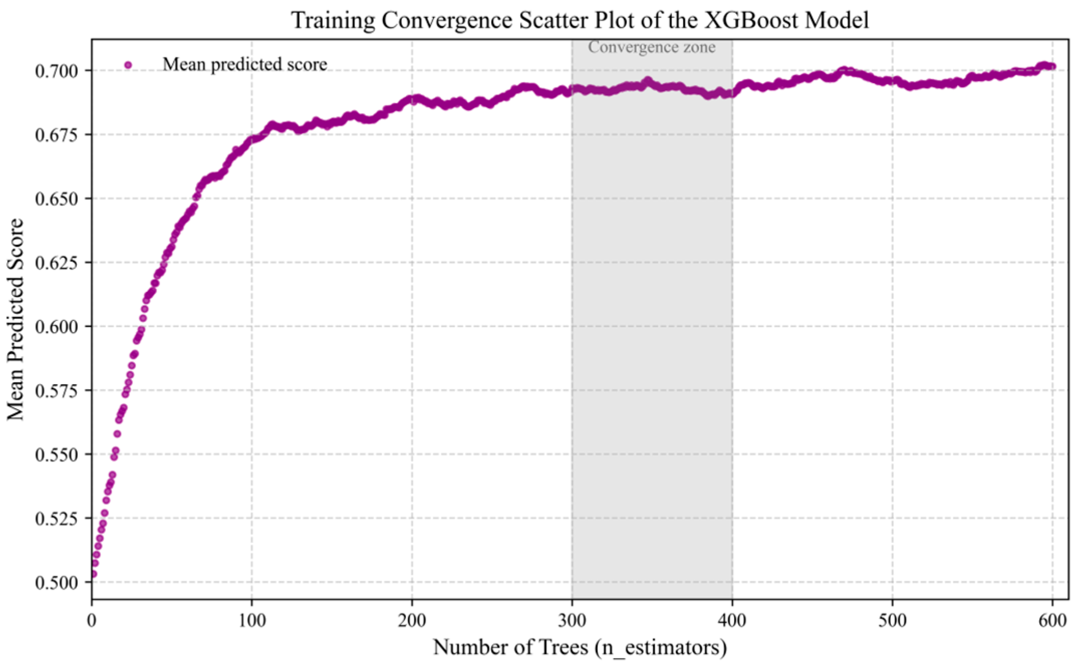
To verify the model’s convergence behavior and training stability, the evolution of the average prediction score was recorded as the number of base learners (CART trees) was incrementally increased. After adding each tree, predictions were generated for the entire sample set, and the average prediction score across all samples was computed. The resulting convergence pattern is illustrated in Figure 4.

Figure 4 illustrates that the model learns rapidly during the initial training phase (first 100 trees), with the average prediction score increasing sharply from approximately 0.50 to around 0.65. This demonstrates the model’s effective capture of essential nonlinear relationships between supplier performance characteristics and risk labels at an early stage. As the number of CART trees grows, performance improvement gradually slows, accompanied by noticeably reduced curve fluctuations. The model enters a stable phase between trees 300 and 400, maintaining an average prediction score near 0.70 with only minor oscillations, indicating convergence has been achieved. Beyond this point, additional trees provide diminishing marginal returns.

Overall, with the current parameter configuration (learning rate: 0.05, maximum depth: 4, n_estimators: 600), the XGBoost model achieves stable convergence within a reasonable number of iterations. The absence of significant overfitting during training confirms that the regularization terms and sampling strategy are appropriately configured. These results validate the model’s strong generalization capability and robustness, confirming its ability to maintain predictive stability while effectively learning patterns from historical data.

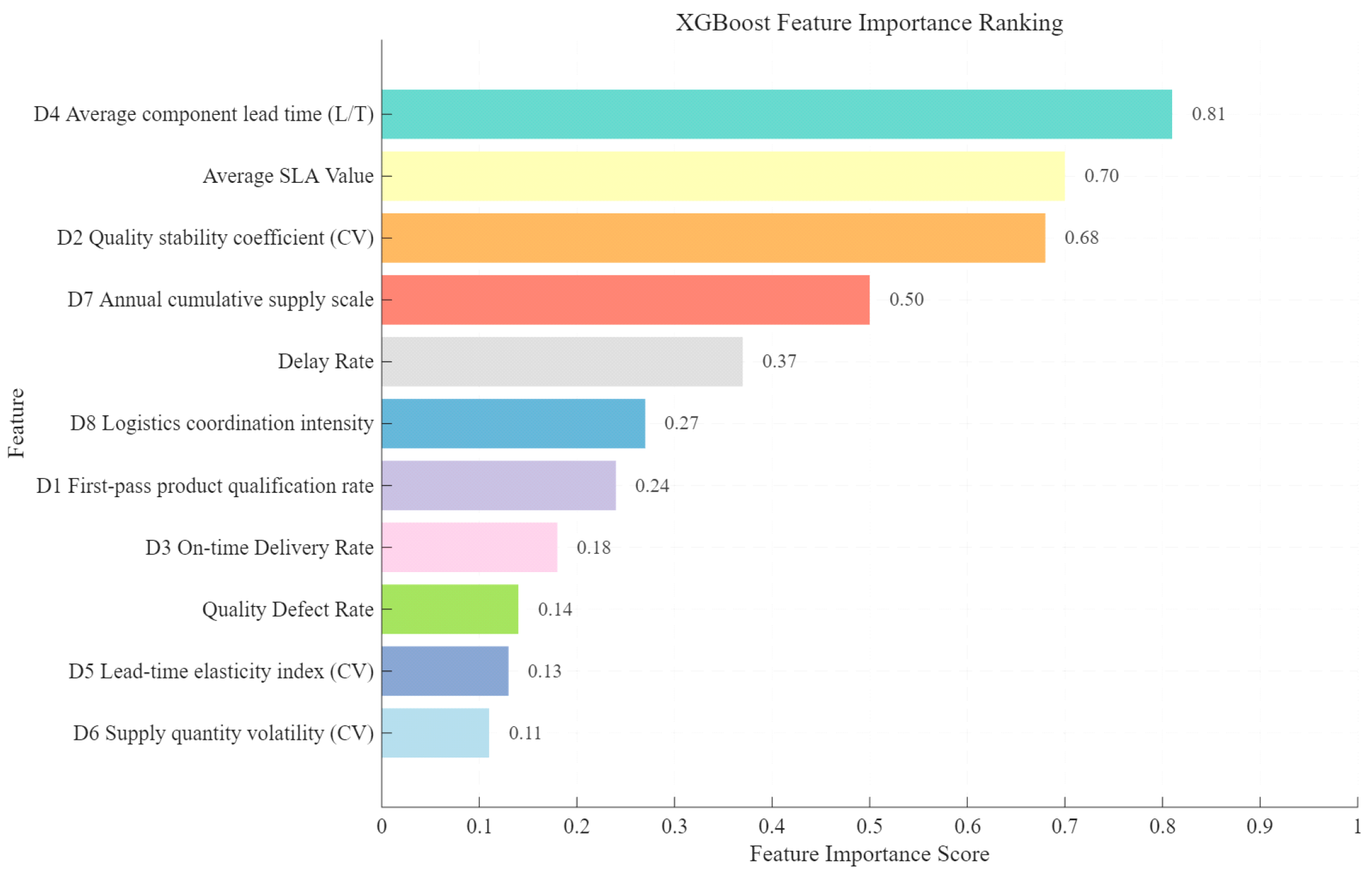
To interpret the model’s predictive mechanism, feature importance scores were computed for all input variables, as shown in the accompanying Figure 5. These scores represent each feature’s relative contribution to the model’s decision-making process, calculated based on the average gain achieved by each feature across all tree structures. While SHAP-based feature importance is used to interpret the XGBoost model, AHP is retained to provide an ex ante, managerially interpretable evaluation structure.

Figure 5 presents the feature importance ranking obtained from the XGBoost model. The results indicate that D4 Average component lead time has the highest importance, suggesting that delivery efficiency is the most critical factor in supplier risk prediction. Extended lead times typically reflect instabilities in production planning, inventory coordination, or logistics execution, thereby increasing the likelihood of subsequent supply disruptions. The average Service Level Agreement (SLA) value ranks second, demonstrating that service fulfillment performance—encompassing delivery timeliness, responsiveness, and issue resolution—provides strong discriminative power for identifying supplier risk. D2 Quality stability coefficient (CV) ranks third, highlighting the importance of quality consistency. Large fluctuations in qualification rates often indicate insufficient process control and elevate the risk of quality-related failures.

D7 Annual cumulative supply scale shows moderate importance, indicating that increasing supply volumes may be associated with higher risk exposure when not matched by corresponding improvements in quality and delivery management. The delay rate and D8 Logistics coordination intensity exhibit comparable importance levels, jointly reflecting short-term delivery reliability and operational coordination with the OEM.

Although D1 First-pass product qualification rate, D3 On-time delivery rate, quality defect rate, D5 Lead-time elasticity index (CV), and D6 Supply quantity volatility (CV) rank relatively lower, they still contribute complementary information through nonlinear feature interactions. Overall, the feature importance distribution shows that the model assigns greater weight to indicators capturing delivery efficiency, service performance, and quality stability, demonstrating the XGBoost model’s ability to identify dominant risk drivers across multiple operational dimensions.

4.4.3. Model Performance Evaluation and Results Analysis

To validate the performance and stability of the developed risk prediction model, this study implemented a grouped five-fold cross-validation (GroupKFold, k = 5) strategy, using the supplier ID as the grouping factor. This validation approach partitions the complete dataset into five mutually exclusive subsets, iteratively using one subset for testing while training on the remaining four. The final performance metrics represent the average across all five iterations. This methodology enables comprehensive utilization of the limited sample data and provides a robust assessment of the model’s generalization capability and stability.

Model performance was evaluated using multiple established metrics: AUC (Area Under the ROC Curve), AP (Average Precision), Precision, Recall, and F1-score, with comparative results summarized in

Table 5. Model performance comparison and validation.

Model	AUC	AP	Precision	Recall
XGBoost	0.851	0.955	0.865	0.978
RandomForest	0.858	0.963	0.846	0.956
Logistic Regression	0.633	0.884	0.818	0.884

. The AUC metric quantifies the model’s overall discriminative power, while AP evaluates its ranking performance specifically for high-risk samples. Precision measures the accuracy of positive predictions, while Recall measures the model’s ability to identify all relevant positive instances (sensitivity). The F1-score provides a balanced representation of both. To prevent information leakage across suppliers, the cross-validation was strictly grouped by supplier_id. This ensures that the performance estimates genuinely reflect the model’s predictive capability on previously unseen suppliers.

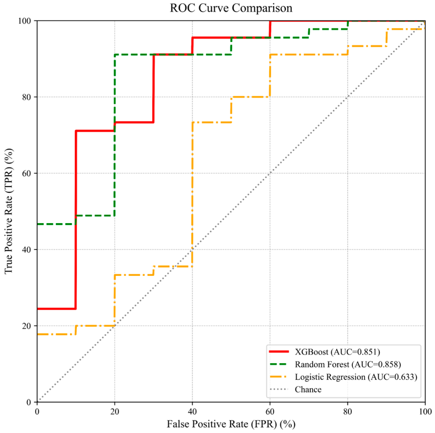
The performance comparison in Table 5 demonstrates that both ensemble tree models, XGBoost and Random Forest, substantially outperform the linear Logistic Regression model. The tree models achieve AUC values exceeding the empirical threshold of 0.85, while Logistic Regression achieves only 0.633, indicating that supplier risk mechanisms involve highly nonlinear patterns that linear models cannot adequately capture. Between the two tree models, Random Forest shows marginal advantages in AUC and AP metrics, which can be attributed to the relatively limited sample size in this case study. As a representative bagging algorithm, Random Forest constructs multiple decision trees through bootstrapped sampling, typically demonstrating enhanced generalization stability with smaller datasets.

However, the primary objective of this research is risk identification, which represents a classic imbalanced classification problem where risk events constitute the minority class. In such contexts, F1-score and Recall generally provide more practical guidance than AUC, since the supply chain impact of missing a high-risk supplier (false negative) significantly exceeds the audit cost of misclassifying a safe supplier (false positive). As shown in Table 5, XGBoost achieves superior performance on these critical risk management metrics, with F1 = 0.928 and Recall = 0.978, compared to Random Forest’s F1 = 0.907 and Recall = 0.956. This performance difference underscores XGBoost’s distinctive advantage as a boosting algorithm; it is specifically designed for iterative optimization and learning from challenging minority-class samples, an advantage further enhanced in this study through the scale_pos_weight parameter. Consequently, it demonstrates exceptional capability in minimizing risk omissions and ensuring comprehensive detection of potential risk events.

The ROC curves presented in Figure 6 provide visual confirmation of these findings. All three models’ curves are positioned substantially above the 45-degree random guessing baseline, confirming the reliability and robustness of the predictions. While the XGBoost and Random Forest curves are closely aligned and both dominate the Logistic Regression curve, indicating comparable overall discriminatory power between the tree-based approaches, XGBoost particularly excels in capturing complex nonlinear relationships among supplier characteristics, especially when multidimensional performance metrics exhibit interaction effects.

Furthermore, to address the class imbalance caused by the low proportion of risk samples in the dataset, the model incorporated a class weight balancing parameter (scale_pos_weight) during training. While this strategy effectively enhances detection of minority-class samples, it may also yield generally elevated risk probability outputs. It is important to note that the model’s output represents a relative confidence score rather than an absolute probability of risk occurrence, indicating the supplier’s likelihood of being classified as high-risk. Overall, the XGBoost model demonstrates superior sensitivity and discriminative power in identifying high-risk suppliers, thereby providing reliable input for subsequent risk-adjusted comprehensive evaluation.

To further examine the robustness and stability of the XGBoost model under the constraint of a limited number of independent suppliers, this study employed a repeated grouped five-fold cross-validation strategy (Repeated GroupKFold, k = 5 with 10 repeats, resulting in 50 validation runs), with supplier IDs strictly used as the grouping factor. This procedure prevents information leakage across suppliers and enables a reliable assessment of performance stability by averaging results over multiple supplier-level partitions.

The performance metrics obtained from the Repeated GroupKFold validation are summarized in

Table 6. Robustness evaluation of the XGBoost model.

Metric	Mean	Std
AUC	0.772	0.026
F1@0.5	0.845	0.022

. The model achieves a mean AUC of 0.772 with a low standard deviation (0.026), together with an F1-score of 0.845 (std = 0.022) at a fixed classification threshold of 0.5. It should be noted that the relatively lower mean AUC observed under the Repeated GroupKFold setting is primarily attributable to the stringent supplier-level data partitioning, which deliberately exposes the model to a wide range of challenging and extreme grouping scenarios. In particular, certain validation folds contain suppliers with highly heterogeneous operational patterns or sparse historical risk events, leading to a more conservative yet realistic estimation of predictive performance. The relatively small variability across repeated runs indicates stable predictive performance that is not sensitive to specific supplier groupings, suggesting a low risk of overfitting despite the modest number of independent supplier entities. This robustness is further supported by the temporally expanded monthly dataset, which captures richer operational dynamics, and by the built-in regularization mechanisms of the XGBoost model.

As a complementary and more stringent generalization test, a Leave-One-Supplier-Out (LOSO) validation was further conducted, in which all records associated with one supplier were held out for testing. The LOSO results yield an average AUC of 0.847, demonstrating that the model maintains effective discriminative capability even when evaluated on completely unseen suppliers. Taken together, these validation results provide strong evidence for the robustness and supplier-level generalization ability of the proposed risk prediction model under realistic data constraints.

Using the trained XGBoost model, predictions were generated for each supplier’s next operational period based on their most recent available monthly data. This process generated model confidence scores reflecting the relative probability of risk events occurring in the subsequent month. The resulting risk prediction rankings are presented in

Table 7. Supplier risk prediction results.

Supplier ID	Risk Confidence Score	Rank
C	0.9731	1
G	0.9673	2
K	0.9634	3
H	0.9512	4
F	0.9511	5
D	0.9507	6
M	0.9497	7
E	0.9286	8
J	0.8843	9
N	0.8296	10
A	0.7235	11
I	0.4841	12
L	0.4841	13
B	0.3310	14

.

4.5. Risk-Adjusted Comprehensive Evaluation Results

While the AHP–TOPSIS model provides a comprehensive evaluation of supplier monthly performance and the XGBoost model quantifies future risk probabilities based on historical data, performance, and risk represent interdependent yet competing dimensions in supply chain management. Relying exclusively on either dimension compromises decision-making rigor. To integrate performance evaluation with risk identification, this study establishes a risk-adjusted evaluation framework that modifies TOPSIS composite scores through risk-based weighting, producing comprehensive scores that reflect both performance levels and risk exposure.

The framework builds upon the comprehensive proximity score $S_i$ derived from the AHP–TOPSIS model, incorporating a risk adjustment factor through Equation (25) to compute the revised comprehensive score $C_i$. With the risk weighting coefficient $\beta$ set to 0.4 to balance performance against risk considerations, the final supplier rankings are presented in

Table 8. Risk-adjusted comprehensive scores and ranking.

Supplier ID	${\mathit{S}}_{\mathit{i}}$	${\widehat{\mathit{P}}}_{\mathit{r}\mathit{i}\mathit{s}\mathit{k}}$	${\mathit{C}}_{\mathit{i}}$	Rank
I	0.5335	0.4841	0.4302	1
L	0.4807	0.4841	0.3876	2
J	0.5585	0.8843	0.3609	3
G	0.5590	0.9673	0.3427	4
H	0.5404	0.9512	0.3348	5
F	0.5142	0.9511	0.3186	6
N	0.4467	0.8296	0.2984	7
E	0.4709	0.9286	0.2960	8
M	0.4767	0.9497	0.2956	9
K	0.4755	0.9634	0.2922	10
D	0.4650	0.9507	0.2882	11
C	0.4554	0.9731	0.2782	12
A	0.3648	0.7235	0.2592	13
B	0.2765	0.3310	0.2399	14

.

The results reveal an approximately 20% reduction in the average comprehensive score after risk adjustment, confirming the risk factor’s effective moderating role on overall ranking. Suppliers exhibiting high static performance but elevated risk confidence experienced a substantial score reduction through the multiplicative penalty term, leading to notable ranking declines. For instance, Supplier G, ranked first in static TOPSIS performance (score: 0.5590), was identified by the XGBoost model as having exceptionally high-risk confidence (second-highest risk score: 0.9673), resulting in its integrated ranking falling to fourth place. Conversely, suppliers with moderate performance but low risk exposure demonstrated relative ranking improvements due to reduced penalty adjustments. Suppliers I and L, originally ranked fourth and sixth in static performance, respectively, achieved first and second positions in the integrated framework owing to their minimal risk adjustments (risk ranks: 12th and 13th).

Consequently, the model’s ranking outcomes align more closely with practical enterprise requirements for procurement, quality, and delivery coordination: high-performance, low-risk suppliers receive preferential recommendation; low-performance, high-risk suppliers are systematically deprioritized; and high-performance, high-risk suppliers are flagged for focused monitoring. In summary, the risk-adjusted framework transforms supplier evaluation from a static assessment to a dynamic, forward-looking approach. This approach not only quantifies historical performance but also proactively identifies future risks, generating evaluation results that better support multidimensional decision-making in complex supply chain environments.

5. Results

The case study results demonstrate that the integrated AHP–TOPSIS–XGBoost model effectively addresses the limitations of traditional supplier rankings, which are based solely on historical performance. The hybrid framework can distinguish discrepancies between suppliers’ past performance and their predicted future risks. Specifically, the model successfully identifies and penalizes potential high-risk suppliers such as G and H, both of which exhibit strong historical performance yet demonstrate elevated predicted risk levels.

In contrast, suppliers such as I and L—characterized by stable performance and controllable risk profiles—are appropriately ranked higher in the risk-adjusted evaluation. These results confirm that the proposed model enables more reliable and robust dual-dimensional decision-making by integrating both performance attributes and predicted risk behaviors. Overall, the findings validate the practical utility and effectiveness of the integrated model in enhancing supplier selection accuracy within the electric vehicle (EV) supply chain environment.

6. Discussion

This study addresses critical challenges in electric vehicle (EV) supply chain management, where traditional Multi-Criteria Decision-Making (MCDM) methods struggle to capture dynamic risks and machine-learning (ML) models often lack interpretability. To bridge this gap, this research proposes an integrated supplier evaluation framework that combines AHP–TOPSIS with XGBoost. The hybrid approach successfully unifies interpretable multidimensional performance assessment with quantitative future risk prediction: the AHP–TOPSIS component provides a transparent performance evaluation structure, while the XGBoost module supplies data-driven forecasts of supplier risk probabilities.

The integrated AHP–TOPSIS–XGBoost model provides EV enterprises with a systematic decision-support tool capable of improving dynamic supplier management and strengthening supply chain resilience. However, to avoid conceptual ambiguity, it is essential to contextualize the role of this model within the broader resilience framework. In supply chain research, resilience typically encompasses both the ability to identify and anticipate risks, as well as the capability to recover and adapt after disruptions. The proposed framework primarily addresses the former by focusing on supplier-level risk identification and early-warning. By dynamically monitoring risk exposure and instability patterns, the model provides decision-makers with timely and interpretable signals that support subsequent resilience-building actions, such as supplier diversification, inventory buffering, or contingency planning. Explicit modeling of post-disruption recovery processes lies beyond the scope of the current study.

In addition, the structural design of this hybrid framework effectively balances the inherent antithesis between operational stability and technological leadership. The AHP–TOPSIS component represents the firm’s strategic anchor, providing a stable performance baseline that ensures consistent supplier management. In contrast, the XGBoost-based predictive module embodies technological leadership by capturing non-linear, dynamic shifts in operational data that static models might overlook. This synergy allows the framework to navigate the contradiction between maintaining long-term supplier relationships and responding to the rapid, often volatile, technological transitions characteristic of the EV industry.

However, several limitations merit consideration. First, the current evaluation relies primarily on internal operational data and does not yet incorporate external risk factors such as geopolitical instability, macroeconomic fluctuations, or raw-material price volatility. While this internal-data-driven configuration ensures data consistency at the enterprise level and reflects direct supplier coordination quality, it may not fully capture macro-level shocks. Importantly, this does not restrict the extensibility of the model, as external indicators can be naturally incorporated as exogenous features within the XGBoost module. Second, the generalization capability of the model may be constrained by the moderate sample size, and the comparative advantages of different ML algorithms require validation using larger-scale datasets. Finally, while the framework captures operational dynamics through rolling updates, the AHP weights used for strategic evaluation remain fixed. In the rapidly evolving EV industry, the relative importance of risk criteria may shift over long-term strategic cycles, and the use of static weights might not fully reflect these macro-level transitions.

Future research should therefore pursue several directions:

• Expanding dataset scope and scale, which will enhance model generalization and enable more comprehensive benchmarking of alternative machine-learning techniques;
• Exploring dynamic weighting mechanisms, such as fuzzy dynamic AHP or entropy-based weight recalibration, to allow the evaluation criteria to evolve in tandem with industry-level strategic shifts;
• Integrating multi-source external data, including macroeconomic indicators, geopolitical information, and news-sentiment analytics, to construct a more dynamic and comprehensive early-warning system for supplier risk.

Such advancements will significantly strengthen the dynamism of risk prediction and improve the universality of the model, offering a more solid technical foundation for building sustainable, resilient, and intelligent supply chain management architectures.

References

- Li, S.; Xie, B. A forewarning model for the reverse supply chain of urban End-of-Life power batteries based on a mix method of BWM and RBFNN. Sci. Rep. 2025, 15, 29883. [Google Scholar] [CrossRef] [Scilit]
- Yan, Q.; Zhang, M.; Li, W.; Qin, G. Risk assessment of new energy vehicle supply chain based on variable weight theory and cloud model: A case study in China. Sustainability 2020, 12, 3150. [Google Scholar] [CrossRef] [Scilit]
- Cheng, A.L.; Fuchs, E.R.; Karplus, V.J.; Michalek, J.J. Electric vehicle battery chemistry affects supply chain disruption vulnerabilities. Nat. Commun. 2024, 15, 2143. [Google Scholar] [CrossRef] [Scilit]
- Liu, X.; Liu, S.; Fu, Z.; Ge, L. A Critical Review of Fault-Tolerant Control for Multiphase PMSM Drive Systems. IEEE Trans. Transp. Electrif. 2025, 11, 13684–13704. [Google Scholar] [CrossRef] [Scilit]
- Ren, H.; Mu, D.; Wang, C.; Yue, X.; Li, Z.; Du, J.; Zhao, L.; Lim, M.K. Vulnerability to geopolitical disruptions of the global electric vehicle lithium-ion battery supply chain network. Comput. Ind. Eng. 2024, 188, 109919. [Google Scholar] [CrossRef] [Scilit]
- Ganguly, K.; Kumar, G. Supply chain risk assessment: A fuzzy AHP approach. Oper. Supply Chain. Manag. Int. J. 2019, 12, 1–13. [Google Scholar] [CrossRef] [Scilit]
- Sharma, V.; Raut, R.D.; Mangla, S.K.; Narkhede, B.E.; Luthra, S.; Gokhale, R. A systematic literature review to integrate lean, agile, resilient, green and sustainable paradigms in the supply chain management. Bus. Strategy Environ. 2021, 30, 1191–1212. [Google Scholar] [CrossRef] [Scilit]
- Abdulla, A.; Baryannis, G. A hybrid multi-criteria decision-making and machine learning approach for explainable supplier selection. Supply Chain. Anal. 2024, 7, 100074. [Google Scholar] [CrossRef] [Scilit]
- Liu, X.; Liu, S.; Dong, Z.; Fu, Z.; Ge, L. An Improved 3-D Space Vector Modulation Strategy for Three-Phase Series-End Winding PMSMs. IEEE Trans. Power Electron. 2025, 40, 15745–15756. [Google Scholar] [CrossRef] [Scilit]
- Rainy, T.A.; Chowdhury, A.R. The Role Of Artificial Intelligence In Vendor Performance Evaluation Within Digital Retail Supply Chains: A Review Of Strategic Decision-Making Models. Am. J. Sch. Res. Innov. 2022, 1, 220–248. [Google Scholar] [CrossRef] [Scilit]
- Ho, W.; Xu, X.; Dey, P.K. Multi-criteria decision making approaches for supplier evaluation and selection: A literature review. Eur. J. Oper. Res. 2010, 202, 16–24. [Google Scholar] [CrossRef] [Scilit]
- Amiri, M.; Hashemi-Tabatabaei, M.; Ghahremanloo, M.; Keshavarz-Ghorabaee, M.; Zavadskas, E.K.; Banaitis, A. A new fuzzy BWM approach for evaluating and selecting a sustainable supplier in supply chain management. Int. J. Sustain. Dev. World Ecol. 2021, 28, 125–142. [Google Scholar] [CrossRef] [Scilit]
- Goodarzi, F.; Abdollahzadeh, V.; Zeinalnezhad, M. An integrated multi-criteria decision-making and multi-objective optimization framework for green supplier evaluation and optimal order allocation under uncertainty. Decis. Anal. J. 2022, 4, 100087. [Google Scholar] [CrossRef] [Scilit]
- Dos Santos, B.M.; Godoy, L.P.; Campos, L.M. Performance evaluation of green suppliers using entropy-TOPSIS-F. J. Clean. Prod. 2019, 207, 498–509. [Google Scholar] [CrossRef] [Scilit]
- Deretarla, Ö.; Erdebilli, B.; Gündoğan, M. An integrated Analytic Hierarchy Process and Complex Proportional Assessment for vendor selection in supply chain management. Decis. Anal. J. 2023, 6, 100155. [Google Scholar] [CrossRef] [Scilit]
- Marzouk, M.; Sabbah, M. AHP-TOPSIS social sustainability approach for selecting supplier in construction supply chain. Clean. Environ. Syst. 2021, 2, 100034. [Google Scholar] [CrossRef] [Scilit]
- Dutta, P.; Jaikumar, B.; Arora, M.S. Applications of data envelopment analysis in supplier selection between 2000 and 2020: A literature review. Ann. Oper. Res. 2022, 315, 1399–1454. [Google Scholar] [CrossRef] [Scilit]
- Vörösmarty, G.; Dobos, I. A literature review of sustainable supplier evaluation with Data Envelopment Analysis. J. Clean. Prod. 2020, 264, 121672. [Google Scholar] [CrossRef] [Scilit]
- Samavati, T.; Badiezadeh, T.; Saen, R.F. Developing double frontier version of dynamic network DEA model: Assessing sustainability of supply chains. Decis. Sci. 2020, 51, 804–829. [Google Scholar] [CrossRef] [Scilit]
- Jahin, M.A.; Naife, S.A.; Saha, A.K.; Mridha, M.F. AI in supply chain risk assessment: A systematic literature review and bibliometric analysis. arXiv 2023, arXiv:2401.10895. [Google Scholar]
- Ali, M.R.; Nipu, S.M.A.; Khan, S.A. A decision support system for classifying supplier selection criteria using machine learning and random forest approach. Decis. Anal. J. 2023, 7, 100238. [Google Scholar] [CrossRef] [Scilit]
- Sani, S.; Xia, H.; Milisavljevic-Syed, J.; Salonitis, K. Supply chain 4.0: A machine learning-based bayesian-optimized LightGBM model for predicting supply chain risk. Machines 2023, 11, 888. [Google Scholar] [CrossRef] [Scilit]
- De Backker, T.; Vercammen, A.; Boute, R.N. A Data-Driven Component Risk Matrix to Assess Supply Chain Disruption Risk. Int. J. Prod. Econ. 2024, in press. [Google Scholar] [CrossRef] [Scilit]
- Gidiagba, O.J.; Tartibu, L.; Okwu, M. Integrating Machine Learning with Multi-Criteria Decision-Making Models for Sustainable Supplier Selection in Dynamic Supply Chains. Logistics 2025, 9, 152. [Google Scholar] [CrossRef] [Scilit]
- Ishizaka, A.; Khan, S.A.; Kheybari, S.; Zaman, S.I. Supplier selection in closed loop pharma supply chain: A novel BWM–GAIA framework. Ann. Oper. Res. 2023, 324, 13–36. [Google Scholar] [CrossRef] [Scilit]
- Galdo, M.I.L.; Miranda, J.T.; Lorenzo, J.M.R.; Caccia, C.G. Internal modifications to optimize pollution and emissions of internal combustion engines through multiple-criteria decision-making and artificial neural networks. Int. J. Environ. Res. Public Health 2021, 18, 12823. [Google Scholar] [CrossRef] [Scilit]
- Saaty, T.L. How to make a decision: The analytic hierarchy process. Eur. J. Oper. Res. 1990, 48, 9–26. [Google Scholar] [CrossRef] [Scilit]
- Tzeng, G.-H.; Huang, J.-J. Multiple Attribute Decision Making: Methods and Applications; CRC Press: Boca Raton, FL, USA, 2011. [Google Scholar]
- Chen, T.; Guestrin, C. Xgboost: A scalable tree boosting system. In Proceedings of the 22nd ACM SIGKDD International Conference on Knowledge Discovery and Data Mining, San Francisco, CA, USA, 13–17 August 2016; pp. 785–794. [Google Scholar]