Research on a Temperature and Humidity Prediction Model for Greenhouse Tomato Based on iT-LSTM-CA

Abstract

Constructing a temperature and humidity prediction model for greenhouse-grown tomatoes is of great significance for achieving resource-efficient and sustainable greenhouse environmental control and promoting healthy tomato growth. However, traditional models often struggle to simultaneously capture long-term temporal trends, short-term local dynamic variations, and the coupling relationships among multiple variables. To address these issues, this study develops an iT-LSTM-CA multi-step prediction model, in which the inverted Transformer (iTransformer, iT) is employed to capture global dependencies across variables and long temporal scales, the Long Short-Term Memory (LSTM) network is utilized to extract short-term local variation patterns, and a cross-attention (CA) mechanism is introduced to dynamically fuse the two types of features. Experimental results show that, compared with models such as Gated Recurrent Unit (GRU), Temporal Convolutional Network (TCN), Recurrent Neural Network (RNN), LSTM, and Bidirectional Long Short-Term Memory (Bi-LSTM), the iT-LSTM-CA achieves the best performance in multi-step forecasting tasks at 3 h, 6 h, 12 h, and 24 h horizons. For temperature prediction, the R² ranges from 0.96 to 0.98, with MAE between 0.42 °C and 0.79 °C and RMSE between 0.58 °C and 1.06 °C; for humidity prediction, the R² ranges from 0.95 to 0.97, with MAE between 1.21% and 2.49% and RMSE between 1.78% and 3.42%. These results indicate that the iT-LSTM-CA model can effectively capture greenhouse environmental variations and provide a scientific basis for environmental control and management in tomato greenhouses.

1. Introduction

Tomato is one of the most important facility-grown crops in China [1], with its cultivation area and yield continuously expanding [2], and the industry scale gradually increasing. However, tomatoes are sensitive to greenhouse environmental conditions during their growth, and fluctuations in temperature and humidity directly affect their growth, flowering, and fruit quality [3,4], thereby having a significant impact on yield and economic benefits. At present, greenhouse environment management largely depends on growers’ experience and manual control, which suffers from delayed responses and limited regulation accuracy, affecting production efficiency. In modern intelligent greenhouse management systems, accurate temperature and humidity prediction is not only a tool for environmental monitoring but also a core component for supporting scientific decision-making. Through high-precision multi-step forecasting, management systems can overcome the lag in greenhouse environmental regulation, shifting from “post-event correction” to “pre-event simulation,” providing forward-looking guidance for automated control equipment. On this basis, combined with real-time monitoring from IoT systems, environmental prediction enables preventive maintenance, reduces the risk of equipment failure [5], and enhances growers’ and related practitioners’ trust and acceptance of smart greenhouse technology [6]. Moreover, by optimizing the microclimate for tomato growth through fine-grained control, it helps improve tomato yield and quality, reduce energy consumption, and promote intelligent resource scheduling and management decision-making in greenhouses.

In greenhouse environment prediction studies, with the deep integration of the Internet of Things (IoT) and automated monitoring technologies in modern agricultural production systems [7], environmental data can be continuously collected, providing a fundamental basis for data-driven predictive modeling. In early studies, traditional time series forecasting methods, such as Back Propagation (BP) neural networks [8] and artificial neural networks (ANN) [9], have been widely used for short-term prediction of greenhouse temperature and humidity. These methods feature simple structures and ease of implementation but exhibit significant limitations in handling long-term dependencies and multivariable relationships. With the development of deep learning, recurrent neural networks (RNN) and their improved models have gradually become the mainstream methods for greenhouse environment prediction. Among them, the LSTM model is widely applied due to its advantage in capturing temporal dependencies. Liu et al. [10] developed an LSTM-based greenhouse climate prediction model, demonstrating its effectiveness in short-term forecasting. Yang et al. [11] introduced a feature attention module (FAM) to further enhance LSTM performance in multi-step prediction tasks. Guo et al. [12] employed a time-position attention LSTM (TPA-LSTM) to achieve multi-step forecasting of temperature and humidity. However, such methods mainly focus on modeling temporal features, and when applied to greenhouse systems characterized by strong nonlinear coupling and significant control lag, they struggle to capture the global evolution trends of environmental factors.

On this basis, researchers have enhanced prediction performance by introducing attention mechanisms or integrating multiple deep learning architectures. Huang et al. [13], addressing the nonlinear and strongly coupled characteristics of edible mushroom greenhouse environments, proposed an A-CNN-LSTM model integrating an attention mechanism, Convolutional Neural Networks (CNN), and LSTM, which significantly outperformed traditional RNN and LSTM models in multi-step prediction of greenhouse temperature, humidity, and CO₂. Shi et al. [14] developed a CNN-LSTM-based greenhouse microclimate prediction model and further optimized the network architecture by incorporating the Sparrow Search Algorithm and SE attention mechanism, resulting in higher prediction accuracy for temperature, humidity, and light intensity. In addition, to further improve prediction performance, some studies applied intelligent optimization algorithms. Zhang Wanfan et al. [15] employed the snake optimization (SO) algorithm to optimize BP neural networks, improving short-term prediction R² and reducing errors. Liang Zhenglong et al. [16] proposed an LSTM–SVM hybrid model, in which future weather information was incorporated to correct prediction results under complex weather conditions, achieving R² values exceeding 0.93. Zulinlu et al. [17] optimized LSTM using the sparrow search algorithm (SSA) to build a daylight greenhouse environment prediction model, achieving an average fit of 97.6% across multiple parameters, including air temperature and humidity, soil temperature and humidity, CO₂, and light. Building upon this, Meng Fanjia et al. [18] further integrated attention mechanisms and employed the SSA algorithm for feature selection and hyperparameter optimization of the LSTM-Attention model, thereby improving the prediction accuracy of multiple factors such as temperature, humidity, and light intensity. However, existing studies based on attention mechanisms or hybrid models still suffer from several limitations. First, most studies adopt self-attention mechanisms that assign weights along the temporal dimension. When the input sequences are long or environmental fluctuations are intense, attention weights tend to be dispersed, making it difficult to accurately disentangle global evolutionary trends from instantaneous local disturbances. Second, multivariate coupling relationships are typically implicitly mapped into high-dimensional feature representations, lacking explicit modeling of the coordinated evolution mechanisms of greenhouse physical factors at the architectural level.

In recent years, Transformer models have been introduced into multivariate time series forecasting tasks due to their advantages in modeling global dependencies through self-attention mechanisms. Li et al. [19] proposed a Transformer-LSTM model that enhances the extraction of long-term dependency features of greenhouse air and soil temperature through self-attention mechanisms. However, conventional Transformers typically embed multiple variables at the same time step as a single token, which somewhat limits their ability to capture global dependencies across variable dimensions. To address this issue, Liu et al. [20] proposed the inverse Transformer (iTransformer) model, which maps the complete historical sequence of each variable into an independent token, constructing attention mechanisms along the variable dimension. This explicitly captures the global correlations among multiple variables while preserving the temporal evolution characteristics of each individual variable. Wang et al. [21] applied the iTransformer to multi-step prediction of greenhouse soil temperature, developing the ReSSA-iTransformer model, which outperformed other models across different temporal scales. Nevertheless, this study primarily focused on a single environmental factor, and further research is needed to model the coordinated evolution features among multivariate environmental factors in detail.

In summary, existing studies have made certain progress in capturing the temporal dependencies of variables such as temperature and humidity, but they still exhibit limitations in modeling the dynamic coupling of multivariate variables while simultaneously accounting for global evolutionary patterns and local disturbances. To address these issues, this study proposes a multi-step forecasting model based on iT-LSTM-CA. The model leverages the iTransformer to map independent variable dimensions into tokens, thereby explicitly capturing the global coupling structure and long-term evolution trends of different factors within the feature space. At the same time, it combines an LSTM network to extract fine-grained local features of instantaneous environmental fluctuations. Finally, a cross-attention mechanism is employed to dynamically integrate global trends and local details. This study aims to provide a predictive basis for intelligent control decision-making in facility-grown tomato greenhouses through multi-step forecasting, while ensuring crop growth and yield, achieving resource-efficient and environmentally friendly management, and promoting greenhouse production toward energy-saving, low-emission, and sustainable development.

2. Materials and Methods

2.1. Experimental Site

The experiment was conducted from 19 September 2024, to 25 January 2025, in Greenhouse No. 4 of an agricultural technology company located in Juye County, Heze City, Shandong Province. The greenhouse is 120 m long from east to west, 12 m wide from north to south, and the rear wall is 3.5 m high. The crop grown inside the greenhouse was tomato, specifically the variety ‘Shuangfei No. 8’. Transplanting took place on 13 September 2024, and the data collection period covered the complete growth cycle of tomatoes, including the seedling stage, flowering and fruit-setting stage, fruit development stage, and harvest stage. The greenhouse was equipped with an automatic ventilation system to ensure suitable environmental conditions for tomato growth.

2.2. IoT-Based Data Acquisition System

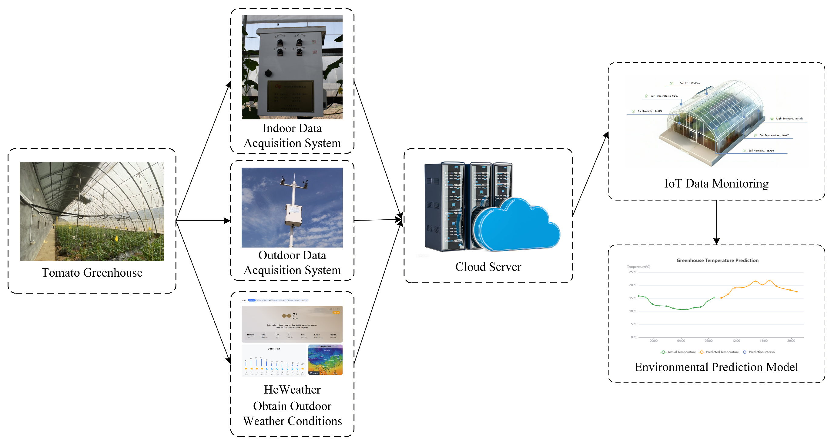
To develop an accurate greenhouse environment prediction model, a distributed multi-source IoT data acquisition system was designed and deployed in this study, as shown in Figure 1. The overall structure of the system follows the sensor deployment principles for protected greenhouses [22], Greenhouse sensors are primarily deployed within the crop growth area. Air temperature, humidity, and light sensors are installed at a height of approximately 1.5 m above the ground to reflect the actual growth conditions of the crops. Soil sensors are buried about 10 cm below the surface to monitor environmental changes in the tomato root zone. Outdoor temperature and humidity sensors are installed in an open area 5 m south of the greenhouse at a height of 2 m above the ground and are equipped with radiation shields to eliminate local heat source interference, ensuring the accuracy of outdoor meteorological data.

The data acquisition frequency of all sensors is 15 min. After digital processing and communication encapsulation through an IoT terminal and a data transmission unit (DTU), the data were uploaded to a cloud server database for storage. The collected environmental parameters included indoor air temperature, indoor air humidity, soil temperature, soil moisture, light intensity, outdoor air temperature, and outdoor air humidity. The sensor specifications are shown in

Table 1. Sensor Parameters.

Sensor Name	Measurement Content	Model	Measuring Range	Accuracy
Air Temperature and Humidity Sensor	Air temperature and humidity	DB-171-30 (Dalian Beifang Measurement and Control Engineering Co., Ltd., Dalian, China)	Temperature: −40–120 °C	±0.1 °C
			Humidity: 0–100%	±1.0%
Soil Temperature and Moisture Sensor	Soil temperature and moisture	TEROS-12 (METER Group, Inc., Pullman, WA, USA)	Temperature: −40–120 °C	±0.1 °C
			Humidity: 0–100%	±0.08%
Light Intensity Sensor	Light intensity	TBQ-6 (Jinzhou Sunshine Meteorological Technology Co., Ltd., Jinzhou, China)	0~200 klux	±0.02 klux

.

In addition, to enhance the model’s ability to perceive external environmental conditions, auxiliary meteorological information was incorporated in this study. Outdoor weather conditions were obtained via the HeWeather API and categorized into classes such as sunny, cloudy, overcast, and rainy according to the weather forecasts, and then transformed into model inputs using numerical encoding.

2.3. Data Processing

2.3.1. Data Preprocessing

To ensure the reliability of subsequent model training and testing, the collected indoor and outdoor environmental data were uniformly aligned and merged according to their temporal characteristics using Python, thereby constructing a structured and multivariate complete dataset.

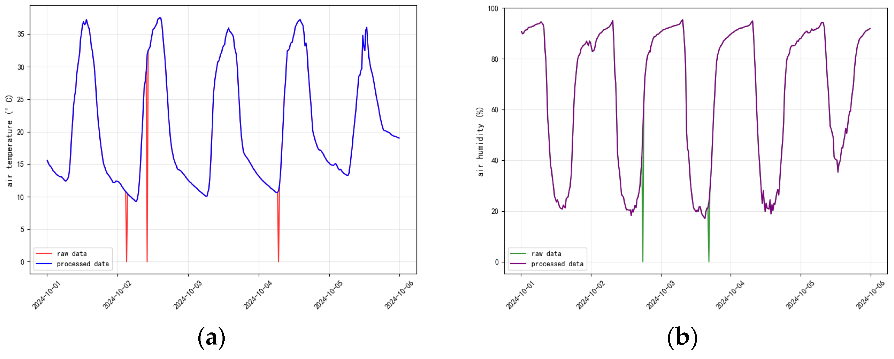
During the IoT data collection process, due to sensor accuracy limitations, network fluctuations, and random noise interference, the raw data contained missing values and outliers. To improve data quality, the study first applied range-limited filtering to identify and remove abnormal points that exceeded physically reasonable thresholds, ensuring that the data conformed to the actual variation patterns of environmental variables. Subsequently, to address missing data caused by temporary sensor failures or communication packet loss, a median-based imputation method [23] was introduced. This method fills missing values using the statistical median of local data, which effectively suppresses residual impulse noise while maintaining the smoothness of the data series and providing stronger robustness against random sensor errors. In this study, a sliding window size of 7 was used. Considering the data sampling frequency of 15 min, this window corresponds to a time span of approximately 105 min. The choice of window size takes into account both the temporal continuity and high inertia characteristics of greenhouse environmental parameters. Within this ~105-min time scale, the physical evolution of temperature and humidity in the greenhouse generally exhibits approximately locally stationary behavior, which helps preserve the local trends of the original series while filling missing values. If the window is too small, the imputation results are easily affected by abnormal sensor noise; if the window is too large, it may excessively smooth the true dynamic variations of the environment, thereby weakening the model’s ability to capture short-term changes. The comparison of partial data before and after preprocessing is shown in Figure 2.

2.3.2. Time Characterization Processing

To enable the model to fully utilize the time series characteristics of greenhouse environmental data, this study carried out characterization processing on the time information. The introduction of time features can help the model identify potential periodic patterns and trend changes in the data, thereby enhancing the stability and accuracy of predictions, and to a certain extent, reducing the impact of noise and occasional anomalies on the model [24].

Considering that environmental parameters usually have obvious daily periodic variations, the time is periodically encoded using sine and cosine functions, and the calculation form is as follows:

$$h_{\sin }=\sin {\displaystyle \frac{2\pi h}{24}}$$

(1)

$$h_{\cos }=\cos {\displaystyle \frac{2\pi h}{24}}$$

(2)

where $h$ represents the hour of the current timestamp, ranging from 0 to 23; $h_{\mathrm{s}\mathrm{i}\mathrm{n}}$ denotes the sine-encoded temporal feature; and $h_{\mathrm{c}\mathrm{o}\mathrm{s}}$ denotes the cosine-encoded temporal feature.

By applying trigonometric transformation to the time information, two new features are generated to capture the periodic variations of environmental parameters within a day. This enhances the model’s ability to perceive and interpret environmental data across different time periods, enabling more accurate prediction of parameter variations in the greenhouse environment.

2.3.3. Data Normalization

To map features with different units and value ranges into a unified interval and improve the stability of backpropagation during model training, the Min–Max normalization method was applied to all input features [25]. The calculation formula is as follows:

$$X_{norm}={\displaystyle \frac{X-X_{min}}{X_{max}-X_{min}}}$$

(3)

In the equation, $X$ represents the raw data, $X_{min}$ denotes the minimum value of the feature across the entire dataset, $X_{\max }$ denotes the maximum value of the feature across the entire dataset, and $X_{\max }-X_{\min }$ is the range, representing the total span of the data. $X-X_{\min }$ represents the deviation of the current value from the minimum, and $X_{\mathrm{norm}}$ is the result of mapping the raw data $X$ into the [0, 1] interval.

2.4. Model Construction

2.4.1. iTransformer Model

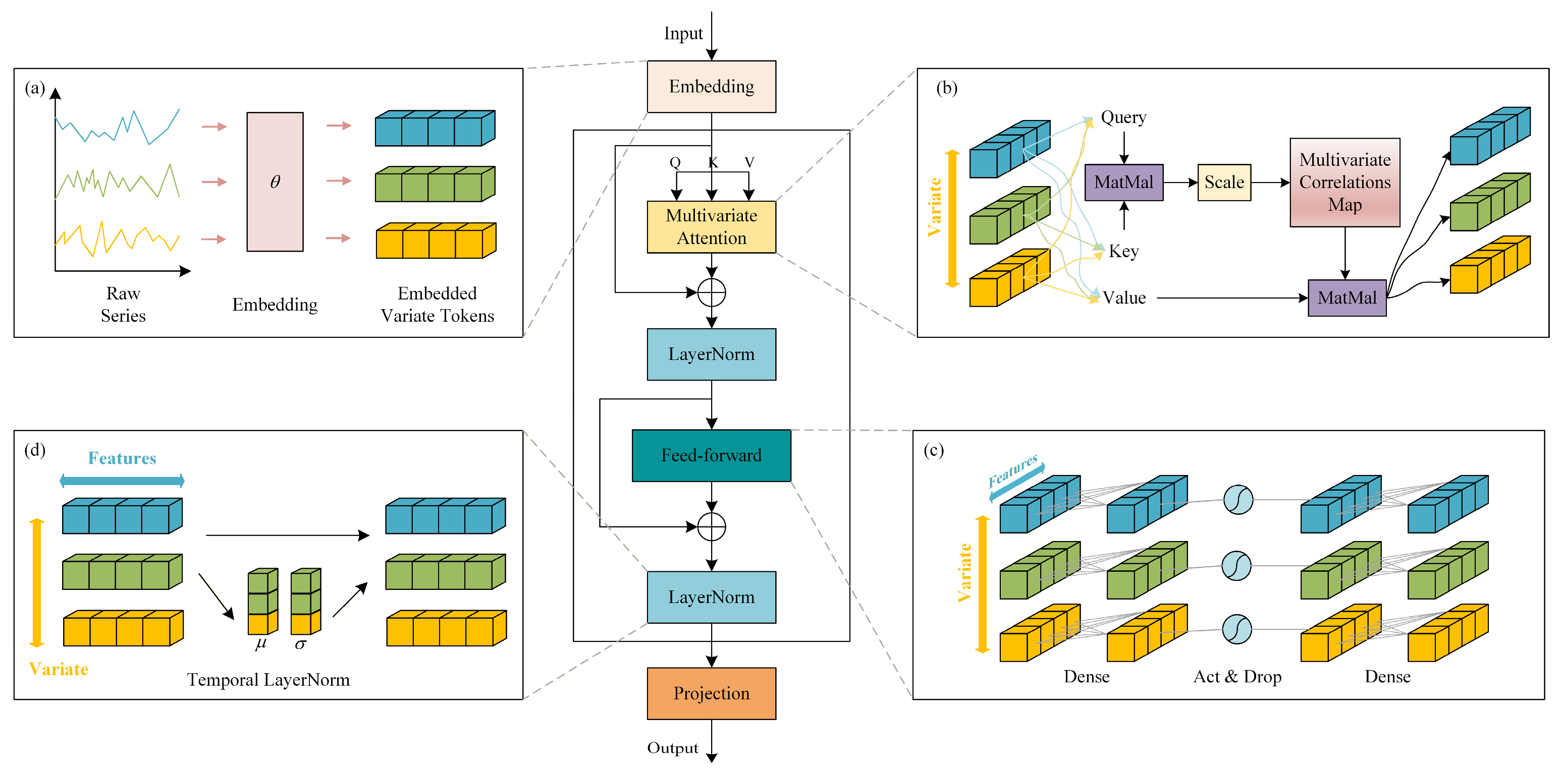
The iTransformer is a novel deep learning model designed for time series forecasting tasks, whose core concept lies in “reversing” the modeling paradigm of the traditional Transformer [21]. The overall architecture is shown in Figure 3. To address the complex coupling characteristics of environmental factors in facility-grown tomato greenhouses, this study treats ten feature dimensions—including indoor and outdoor air temperature and humidity, soil temperature and humidity, light intensity, weather conditions, and time-periodic features such as hsin and hcos—as independent tokens using the iTransformer.

Unlike conventional Transformers, which treat time steps as tokens, the iTransformer performs self-attention modeling along the feature dimensions. This design explicitly captures the correlations among different physical variables, thereby constructing the global dependency structure of the greenhouse microclimate system at a macro level. The specific mechanism of the model is as follows:

(i)

Embedding Layer. The temporal sequences of each environmental factor within the input window (L = 48) are mapped into continuous high-dimensional dense vectors. In this study, sequences such as indoor temperature and light intensity are independently encoded as feature tokens. This approach preserves the unique evolutionary information of each factor and provides fine-grained feature representations for subsequent modeling of interactions among variables.

(ii)

Transformer Module. It consists of three components: multivariate attention mechanism, feedforward neural network (FFN), and layer normalization.

Multivariate Attention Mechanism: Applied to the ten embedded environmental feature tokens. By computing attention weights among factors, the model can learn cross-variable physical constraints within the greenhouse system from a global perspective

Feedforward Neural Network (FFN): Performs deep nonlinear transformations on each environmental feature token, further extracting complex nonlinear evolution patterns in the temperature, humidity, and soil parameter sequences.

Layer Normalization: Normalizes the feature tokens, effectively addressing the issue of large numerical differences among variables with different physical dimensions and ensuring convergence during deep network training.

(iii)

Projector Layer. A multilayer perceptron maps the learned high-dimensional feature tokens to the length of the prediction target sequence ($H\in \{12,24,48,96\}$). This layer realizes a direct mapping from the global feature space to future time steps. The resulting global representations capture environmental evolution trends under the coordinated influence of multiple factors, providing support for subsequent integration with local features.

2.4.2. LSTM Neural Network Model

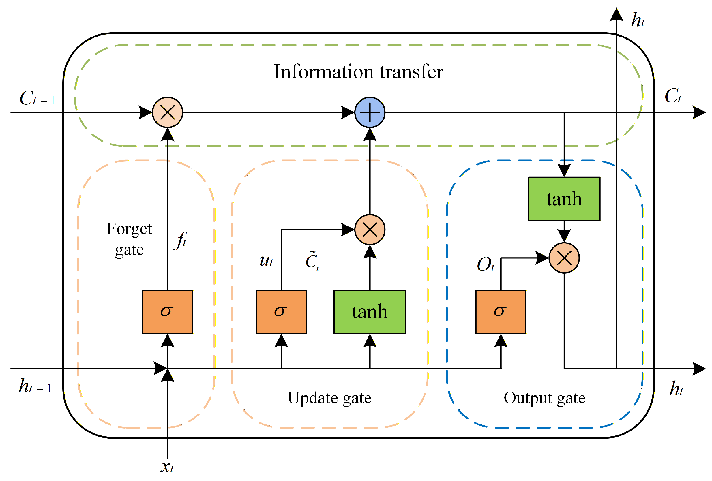
The Long Short-Term Memory (LSTM) network was first proposed by Hochreiter and Schmidhuber in 1997 [26], with the primary aim of addressing the vanishing and exploding gradient problems commonly encountered in traditional recurrent neural networks (RNNs) when processing long sequences [27]. Compared with conventional RNNs, LSTM introduces gating mechanisms and a cell state, enabling it to effectively capture long-term dependencies in sequences while suppressing the interference of irrelevant information during network training.

In this study, the LSTM module is primarily used to capture the local dynamic features of greenhouse environmental data, complementing the global trend features extracted by the iTransformer. Facility-grown tomato greenhouses are influenced by manual operations, which may cause non-stationary impulse fluctuations over short periods. The LSTM leverages its gating mechanisms to model these short-term disturbances at a fine-grained level, thereby enhancing the model’s sensitivity to short-term variations.

As shown in Figure 4, the LSTM processes multivariate features at each time step through the coordinated operation of the forget gate ($f_t$), input gate ($u_t$), cell state, and output gate ($o_t$), effectively preserving local instantaneous variation information.

The model adopts a two-layer stacked LSTM architecture to enhance its capacity for fitting nonlinear fluctuations. The input consists of preprocessed greenhouse environmental sequences $X\in {\mathbb{R}}^{L\times D}$ (L = 48, D = 10), from which hidden state vectors $h_t$ are generated iteratively through the hidden layers. These vectors serve as local feature representations, reflecting not only the short-term temporal variations of temperature and humidity but also providing support for subsequent cross-attention fusion with global trend features.

2.4.3. Cross-Attention Mechanism

Cross-attention (CA) is an important mechanism in the Transformer architecture for enabling information interaction between different feature sequences [28]. Unlike self-attention, which computes correlations only within the same sequence, cross-attention introduces two independent input sequences, allowing the model to establish relationships between data from different sources.

In this study, the local dynamic features extracted by the LSTM module are mapped to the Query (Q), while the global features extracted by the iTransformer are mapped to the Key (K) and Value (V). This allocation ensures that the model can use local short-term fluctuations as the index to dynamically weight global trend information, thereby maintaining sensitivity to instantaneous disturbances. If the assignment is reversed (global features as Q and local features as K/V), the model tends to overlook local variations, resulting in lagged or dampened predictions.

Cross-attention generates a weight distribution by computing the similarity between Q and K and performs a weighted sum over V, enabling adaptive modulation of global features based on local features. The computation is formulated as follows:

$$\mathrm{Attention}(Q,K,V)=\mathrm{softmax}\left({\displaystyle \frac{Q{K}^{\mathcal{T}}}{\sqrt{d_k}}}\right)V$$

(4)

Here, $Q=X_1{W}^Q$, $K=V=X_2{W}^K$, where $X_1$ and $X_2$ denote the input feature matrices from the LSTM and iTransformer pathways, respectively; $W^Q$ and $W^K$ are the weight matrices, and $d_k$ represents the dimension of the key vectors.

Through this mechanism, the model can achieve adaptive fusion of local dynamic information and global trend constraints during prediction. This enables the model to remain sensitive to short-term fluctuations while adhering to the overall evolutionary patterns of the greenhouse environment system, thereby realizing a synergistic representation of multi-scale features.

2.4.4. iT-LSTM-CA Prediction Model

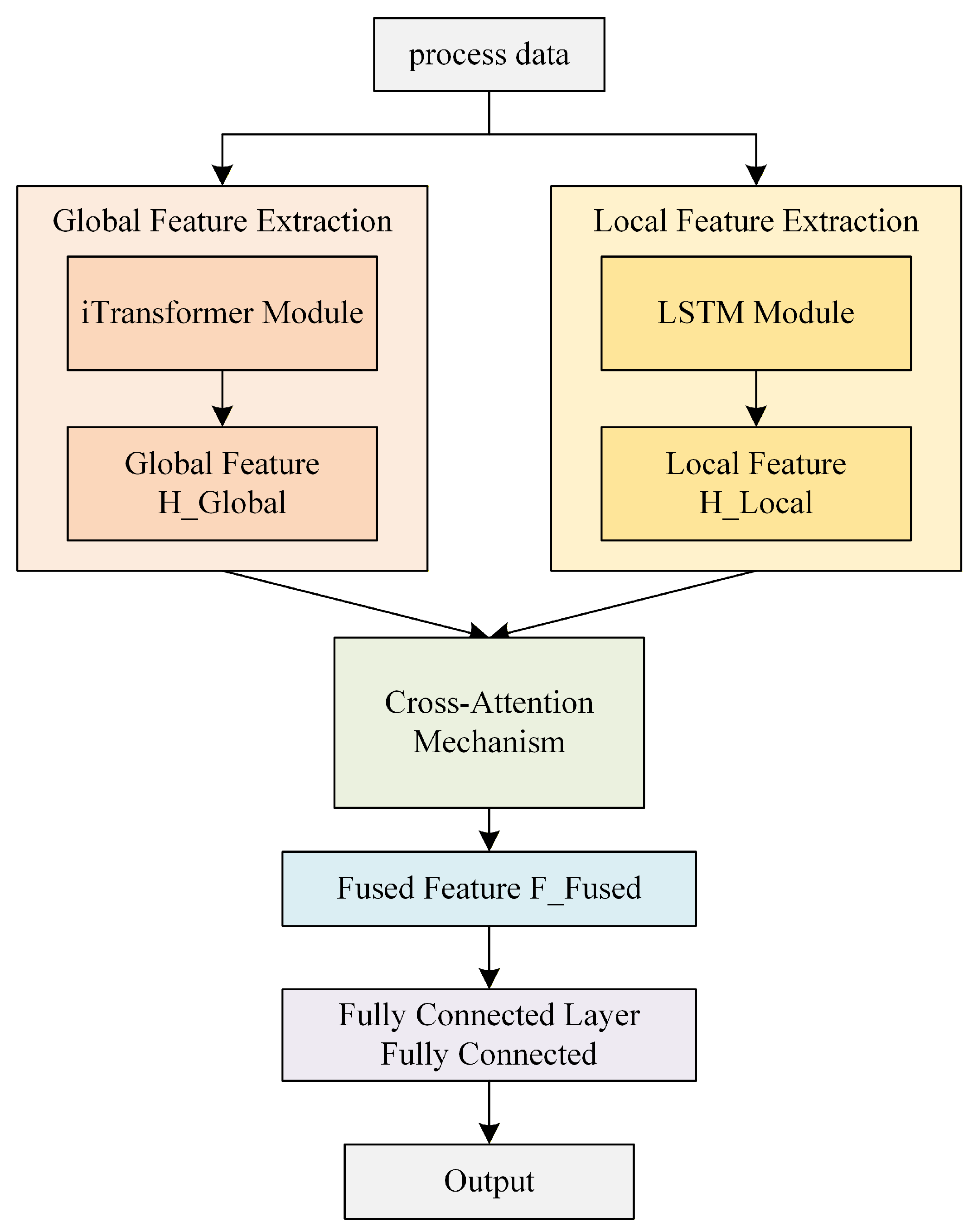
Based on the aforementioned modules, this study proposes the iT-LSTM-CA model for multi-step prediction of greenhouse temperature and humidity. The overall architecture is shown in Figure 5.

The model workflow is as follows:

(i)

Model input: The input tensor is $X\in {\mathbb{R}}^{B\times L\times D}$, where the batch size $B=32$, input window length $L=48$, and feature dimension $D=10$. All input data are normalized using Min-Max scaling to eliminate differences in measurement units.

(ii)

Global and local paths:

Global path: The input tensor is transposed along the feature dimension, treating each feature as a token, and fed into the iTransformer encoder (single-layer structure with 8 attention heads and 512 channels) to model global dependencies among environmental factors.

Local path: The original temporal tensor is simultaneously fed into a two-layer stacked LSTM module (hidden units 128 and 256, with Dropout = 0.2) to capture instantaneous nonlinear fluctuations through its gating mechanisms.

(iii)

Cross-attention: The local dynamic representations serve as the Query (Q), while the global trend representations serve as the Key (K) and Value (V). By computing the attention weight distribution between Q and K, the model adaptively selects and fuses local dynamic features with global trend features.

(iv)

Projection and output: The fused feature vectors are linearly transformed through the Projector layer, mapping the high-dimensional features to the prediction target length. The model ultimately outputs the prediction tensor $Y\in {\mathbb{R}}^{B\times H\times 2}$, where $H\in \{12,24,48,96\}$ corresponds to predicted values of indoor air temperature and humidity for the next 3 h, 6 h, 12 h, and 24 h, respectively.

2.5. Evaluation Metrics

In this study, the model’s prediction performance was evaluated using Mean Absolute Error (MAE), Root Mean Square Error (RMSE), and the Coefficient of Determination (R²).

$$RMSE=\sqrt{{\displaystyle \frac{1}{N}}\sum _{i=1}^N{\left(x_i-y_i\right)}^2}$$

(5)

$$MAE={\displaystyle \frac{1}{N}}\sum _{i=1}^N|x_i-y_i|$$

(6)

$$R^2=1-{\displaystyle \frac{{\displaystyle \sum _{i=1}^N}{(x_i-y_i)}^2}{{\displaystyle \sum _{i=1}^N}{({\overline{y}}_i-y_i)}^2}}$$

(7)

3. Results

3.1. Experimental Environment and Parameter Configuration

The experiments were conducted based on the PyTorch 1.13.0 + cu117 deep learning framework. The specific hardware and software environment configurations are shown in

Table 2. Experimental Environment Configuration.

Configuration	Parameter
Operating System	Windows 11
CPU	Intel Core i7-13700F
GPU	GeForce RTX 4070
Framework	Pytorch 1.13.0 + cu117
Programming Language	Python 3.8

.

The greenhouse environment time series data were divided sequentially, with 70% used for the training set, 15% for the validation set, and 15% for the test set. To ensure the fairness and objectivity of the comparative experiments, this study adopts a strategy of ‘aligning task-related parameters while independently optimizing structural parameters’.

First, the global task-related parameters of all models were unified: the learning rate was set to 0.001, the Adam optimizer was used, the batch size was 32, the number of training epochs was 150, and the input window length was fixed at 48. The training process for all models used mean squared error (MSE) as the loss function. Second, the core hyperparameters specific to each model’s structural characteristics were independently optimized through trial-and-error and grid search to ensure that all baseline models achieve their optimal performance. The configuration of the proposed iT-LSTM-CA model is as follows: the LSTM module adopts a two-layer stacked architecture with hidden units of 128 and 256, and a dropout rate of 0.2; the iTransformer encoder uses a single-layer structure with 8 attention heads, 512 channels, and GELU as the activation function. For comparison models such as RNN and GRU, the hidden layer dimensions and attention mechanism parameters were selected as the optimal values within their respective search spaces.

To evaluate the model’s generalization ability at different prediction horizons, multi-step forecasting tasks were designed, including t+12 (3 h), t+24 (6 h), t+48 (12 h), and t+96 (24 h), providing a comprehensive assessment of the model’s performance in both short-term and mid- to long-term predictions.

3.2. Analysis of Data Preprocessing Strategies

To evaluate the effectiveness of the sliding-window median imputation method for greenhouse IoT data, this study compared three commonly used missing value handling methods: linear interpolation, forward filling, and sliding-window median imputation. Different proportions of data loss (5%, 10%, and 20%) were randomly simulated in the original complete dataset, and each method was applied for imputation. The imputation performance was quantified using mean squared error (MSE).

As shown in

Table 3. Evaluation of Different Missing Value Handling Methods.

Missing Ratio	Imputation Method	Temperature MSE (°C)	Humidity MSE (%)
5%	Linear Interpolation	0.06	0.51
	Forward Filling	0.42	3.66
	Sliding-Window Median	0.01	0.18
10%	Linear Interpolation	0.08	0.79
	Forward Filling	0.34	3.18
	Sliding-Window Median	0.02	0.34
20%	Linear Interpolation	1.59	12.31
	Forward Filling	1.56	11.91
	Sliding-Window Median	0.31	2.29

, the sliding-window median imputation method effectively restores missing data across all missing ratios, while preserving the local variation trends of greenhouse environmental parameters and exhibiting strong robustness to outliers. Under 5% missing data, the MSEs for temperature and humidity were 0.01 °C and 0.18%, respectively; even with 20% missing data, the MSEs remained 0.31 °C and 2.29%. In contrast, linear interpolation and forward filling exhibited larger errors at higher missing ratios, especially for the humidity variable, whose high volatility makes simple imputation methods inadequate for accurate restoration.

Based on the above results, this study adopts the sliding-window median imputation method for preprocessing the raw data.

3.3. Analysis of iTransformer Hyperparameters

To evaluate the effects of the iTransformer module’s number of layers and attention heads on model performance, this study conducted comparative experiments under fixed global training parameters (learning rate = 0.001, Adam optimizer, batch size = 32, 150 training epochs, and input window length = 48). The impact of the iTransformer’s layer number and attention heads on the overall model’s predictive performance was assessed using the temperature prediction task as an example, with results shown in

Table 4. Analysis of Key Hyperparameters of the iTransformer Module (Using Temperature Prediction as an Example).

Layers	Attention Heads	3 h			6 h			12 h			24 h
		MAE/°C	RMSE/°C	R2	MAE/°C	RMSE/°C	R2	MAE/°C	RMSE/°C	R2	MAE/°C	RMSE/°C	R2
1	1	0.51	0.67	0.58	0.75	0.74	0.95	0.85	1.15	13.24	0.51	0.67	0.58
1	4	0.46	0.62	0.52	0.68	0.70	0.88	0.81	1.10	15.42	0.46	0.62	0.52
1	8	0.42	0.58	0.48	0.64	0.67	0.84	0.79	1.06	17.15	0.42	0.58	0.48
2	8	0.42	0.58	0.48	0.64	0.67	0.83	0.79	1.05	32.48	0.42	0.58	0.48
3	8	0.42	0.58	0.48	0.64	0.66	0.83	0.78	1.05	63.92	0.42	0.58	0.48

.

The results indicate that increasing the number of attention heads significantly improves short-term prediction performance. With the number of layers fixed at one, increasing attention heads from 1 to 8 reduced the 3-h prediction MAE from 0.51 °C to 0.42 °C and RMSE from 0.67 °C to 0.58 °C, while the errors for medium- and long-term predictions (12 h and 24 h) also slightly decreased, suggesting that more attention heads help the model capture both local and global features simultaneously.

When the number of heads was fixed, increasing the number of layers had little effect on short-term predictions and only marginally improved medium- and long-term predictions. The 3-h prediction MAE remained stable across 1–3 layers, while the 24-h MAE slightly decreased from 1.06 °C to 1.05 °C; however, training time increased from 17.15 s/epoch to 63.92 s/epoch, indicating that adding layers increases computational cost.

Considering both predictive performance and training efficiency, this study ultimately selected 1 layer with 8 attention heads as the iTransformer module’s hyperparameter setting, balancing model accuracy and training cost.

3.4. Ablation Study

To evaluate the contribution of each module within the iT-LSTM-CA model, an ablation study was conducted. To minimize the impact of neural network training randomness on the experimental results, all models were independently run 5 times under the same experimental environment and parameter settings, and the mean and standard deviation of the results were calculated for statistical analysis.

At four prediction horizons—3 h, 6 h, 12 h, and 24 h—the performance of different module combinations in greenhouse temperature and humidity forecasting was compared. The results are shown in

Table 5. Ablation study results for temperature prediction across different forecasting horizons.

Model	Indicator	3 h	6 h	12 h	24 h	Params (M)	FLOPs (G)
LSTM	MAE/°C	0.71 ± 0.04	0.85 ± 0.05	0.92 ± 0.07	1.18 ± 0.09	0.42	0.85
	RMSE/°C	0.91 ± 0.05	1.07 ± 0.07	1.24 ± 0.09	1.56 ± 0.13
	R2	0.96	0.96	0.95	0.94
iTransformer	MAE/°C	0.75 ± 0.04	0.89 ± 0.05	0.90 ± 0.06	0.95 ± 0.08	0.36	0.62
	RMSE/°C	0.95 ± 0.06	1.12 ± 0.08	1.20 ± 0.09	1.38 ± 0.11
	R2	0.95	0.94	0.94	0.94
LSTM + iTransformer	MAE/°C	0.51 ± 0.03	0.66 ± 0.04	0.79 ± 0.06	0.90 ± 0.07	0.78	1.47
	RMSE/°C	0.67 ± 0.04	0.87 ± 0.05	1.15 ± 0.08	1.25 ± 0.11
	R2	0.97	0.97	0.96	0.95
LSTM + iTransformer + Cross-Attention (Q = Global, K/V = Local)	MAE/°C	0.49 ± 0.03	0.58 ± 0.04	0.76 ± 0.05	0.88 ± 0.08	0.84	1.65
	RMSE/°C	0.66 ± 0.04	0.76 ± 0.05	1.02 ± 0.08	1.21 ± 0.11
	R2	0.97	0.96	0.96	0.95
LSTM + iTransformer + Cross-Attention (Q = Local, K/V = Global)	MAE/°C	0.42 ± 0.01 *	0.48 ± 0.02 *	0.67 ± 0.03 *	0.79 ± 0.05 *	0.84	1.65
	RMSE/°C	0.58 ± 0.02 *	0.64 ± 0.02 *	0.84 ± 0.04 *	1.06 ± 0.07 *
	R2	0.98	0.98	0.97	0.96

* indicates a statistically significant improvement in temperature prediction compared with the LSTM + iTransformer fusion model (p < 0.05).

and

Table 6. Ablation study results for humidity prediction across different forecasting horizons.

Model	Indicator	3 h	6 h	12 h	24 h	Params (M)	FLOPs (G)
LSTM	MAE/%	2.25 ± 0.09	2.76 ± 0.12	3.21 ± 0.15	3.87 ± 0.22	0.42	0.85
	RMSE/%	3.15 ± 0.12	3.62 ± 0.15	4.85 ± 0.22	5.24 ± 0.32
	R2	0.94	0.93	0.92	0.91
iTransformer	MAE/%	2.45 ± 0.11	2.95 ± 0.13	3.07 ± 0.14	3.65 ± 0.18	0.36	0.62
	RMSE/%	3.40 ± 0.14	3.85 ± 0.17	4.61 ± 0.22	4.92 ± 0.28
	R2	0.93	0.93	0.93	0.92
LSTM + iTransformer	MAE/%	1.59 ± 0.07	2.13 ± 0.11	2.41 ± 0.12	2.84 ± 0.14	0.78	1.47
	RMSE/%	2.26 ± 0.12	3.19 ± 0.15	3.95 ± 0.18	4.12 ± 0.22
	R2	0.95	0.94	0.94	0.93
LSTM + iTransformer + Cross-Attention (Q = Global, K/V = Local)	MAE/%	1.48 ± 0.08	1.98 ± 0.10	2.35 ± 0.11	2.78 ± 0.14	0.84	1.65
	RMSE/%	2.15 ± 0.11	2.88 ± 0.15	3.72 ± 0.21	4.01 ± 0.25
	R2	0.96	0.95	0.94	0.94
LSTM + iTransformer + Cross-Attention (Q = Local, K/V = Global)	MAE/%	1.21 ± 0.04 *	1.64 ± 0.05 *	2.04 ± 0.07 *	2.49 ± 0.09 *	0.84	1.65
	RMSE/%	1.78 ± 0.06 *	2.31 ± 0.08 *	3.11 ± 0.12 *	3.42 ± 0.15 *
	R2	0.97	0.96	0.95	0.95

* indicates a statistically significant improvement in humidity prediction compared with the LSTM + iTransformer fusion model (p < 0.05).

. The experimental results indicate that, for greenhouse temperature prediction, using the LSTM model alone yields MAEs of 0.71 °C, 0.85 °C, 0.92 °C, and 1.18 °C for the 3-h, 6-h, 12-h, and 24-h prediction steps, respectively. When using the iTransformer model alone, the corresponding MAEs are 0.75 °C, 0.89 °C, 0.90 °C, and 0.95 °C. Although both standalone models demonstrate certain predictive capability, they exhibit clear limitations: the LSTM model excels at capturing local temporal patterns, whereas the iTransformer model is superior in extracting global dependencies. However, each model is relatively insufficient in the complementary dimension.

After simply combining LSTM and iTransformer, the model achieves performance superior to either standalone model at all prediction horizons. At the 3-h horizon, the MAE for temperature prediction decreases from the best standalone value of 0.71 °C to 0.51 °C, and the RMSE decreases from 0.91 °C to 0.67 °C. For humidity prediction, the MAE decreases from the best standalone value of 2.25% to 1.59%, and the RMSE decreases from 3.15% to 2.26%. Aside from the 3-h horizon, this fused model also achieves varying degrees of improvement at the 6-h, 12-h, and 24-h steps. The above results indicate that the simple fusion of LSTM and iTransformer enhances the overall predictive capability of the model.

Building upon this fusion, the cross-attention (CA) mechanism was further introduced to investigate the impact of CA module design on performance. Two feature interaction schemes were compared: (1) using local features as the Query and global features as Key/Value, and (2) using global features as the Query and local features as Key/Value. The results demonstrate that using local Query consistently outperforms the global Query scheme in both temperature and humidity prediction tasks. Specifically, for temperature prediction, the MAE at 3 h, 6 h, 12 h, and 24 h are 0.42 °C, 0.48 °C, 0.67 °C, and 0.79 °C, respectively, compared with 0.49 °C, 0.58 °C, 0.76 °C, and 0.88 °C for the global Query scheme. For humidity prediction, the MAE values are 1.21%, 1.64%, 2.04%, and 2.49%, outperforming the corresponding global Query values of 1.48%, 1.98%, 2.35%, and 2.78%. These results highlight the effectiveness of the CA module with local Query in leveraging local dynamic features to adaptively refine global trend information, thereby further improving predictive accuracy.

To quantify the reliability of the performance improvement, a paired t-test was conducted between the iT-LSTM-CA model with local Query/global Key-Value and the simple LSTM + iTransformer fusion model. The results show that for all prediction horizons of temperature and humidity, both MAE and RMSE exhibit statistically significant differences (p < 0.05), indicating that the observed performance gains are not due to random training fluctuations. Moreover, the mean and standard deviation obtained from multiple independent trainings demonstrate that the introduction of the CA module stabilizes model performance, particularly at longer prediction horizons.

In terms of computational overhead, the inclusion of the CA module increases the model parameters by approximately 0.06 M and the FLOPs by about 0.18 G. However, both temperature and humidity prediction accuracy are significantly improved, suggesting that the performance gains outweigh the additional computational cost.

In summary, the iT-LSTM-CA model captures global dependencies via the iTransformer module, extracts local features through the LSTM module, and dynamically integrates them using the cross-attention mechanism, thereby establishing a multi-level framework for feature extraction and fusion.

To evaluate the actual contribution of weather category features to model predictive performance, ablation experiments were conducted comparing model predictions with and without the inclusion of weather category features. The results are shown in

Table 7. Ablation Experiment on Weather Category Features: Temperature Prediction.

Model	3 h			6 h			12 h			24 h
	MAE/°C	RMSE/°C	R2	MAE/°C	RMSE/°C	R2	MAE/°C	RMSE/°C	R2	MAE/°C	RMSE/°C	R2
iT-LSTM-CA (w/o weather)	0.46 ± 0.02	0.63 ± 0.03	0.97	0.53 ± 0.03	0.71 ± 0.04	0.97	0.73 ± 0.03	0.89 ± 0.04	0.96	0.87 ± 0.06	1.12 ± 0.09	0.95
iT-LSTM-CA (with weather)	0.42 ± 0.01	0.58 ± 0.02	0.98	0.48 ± 0.02	0.64 ± 0.02	0.98	0.67 ± 0.03	0.84 ± 0.04	0.97	0.79 ± 0.05	1.06 ± 0.07	0.96

and

Table 8. Ablation Experiment on Weather Category Features: Humidity Prediction.

Model	3 h			6 h			12 h			24 h
	MAE/%	RMSE/%	R2	MAE/%	RMSE/%	R2	MAE/%	RMSE/%	R2	MAE/%	RMSE/%	R2
iT-LSTM-CA (w/o weather)	1.28 ± 0.05	1.87 ± 0.06	0.96	1.72 ± 0.06	2.39 ± 0.08	0.95	2.13 ± 0.07	3.18 ± 0.11	0.94	2.61 ± 0.09	3.54 ± 0.14	0.94
iT-LSTM-CA (with weather)	1.21 ± 0.04	1.78 ± 0.06	0.97	1.64 ± 0.05	2.31 ± 0.08	0.96	2.04 ± 0.07	3.11 ± 0.12	0.95	2.49 ± 0.09	3.42 ± 0.15	0.95

. The results indicate that incorporating weather features reduces the MAE for temperature prediction by approximately 0.04–0.08 °C across all horizons, and reduces the MAE for humidity prediction by about 0.07–0.12%, while slightly increasing R². This suggests that weather category information can improve the model’s predictive capability to a certain extent.

3.5. Comparative Analysis

To verify the effectiveness of the proposed iT-LSTM-CA temperature and humidity prediction model, a comparative analysis was conducted on six models under four prediction horizons for both temperature and humidity forecasting.

As shown in

Table 9. Comparison results of temperature prediction by different models.

Model	3 h			6 h			12 h			24 h
	MAE/°C	RMSE/°C	R2	MAE/°C	RMSE/°C	R2	MAE/°C	RMSE/°C	R2	MAE/°C	RMSE/°C	R2
GRU	0.73	0.94	0.95	0.88	1.10	0.95	0.96	1.28	0.94	1.22	1.61	0.93
TCN	0.69	0.89	0.96	0.83	1.05	0.95	0.91	1.22	0.95	1.15	1.52	0.94
RNN	0.82	1.05	0.93	0.97	1.23	0.92	1.08	1.42	0.91	1.35	1.78	0.89
LSTM	0.71	0.91	0.96	0.85	1.07	0.96	0.92	1.24	0.95	1.18	1.56	0.94
Bi-LSTM	0.68	0.87	0.96	0.81	1.03	0.96	0.89	1.19	0.95	1.12	1.48	0.94
iTransformer	0.75	0.95	0.95	0.89	1.12	0.94	0.90	1.20	0.94	0.95	1.38	0.94
DLinear	0.68	0.86	0.96	0.82	1.06	0.95	0.93	1.25	0.94	1.18	1.58	0.93
PatchTST	0.61	0.83	0.97	0.72	0.93	0.97	0.78	1.04	0.96	0.87	1.25	0.95
iT-LSTM-CA	0.42	0.58	0.98	0.48	0.64	0.98	0.67	0.84	0.97	0.79	1.06	0.96

, in terms of temperature prediction, the traditional RNN model exhibits relatively high MAE and RMSE and comparatively low R² across different horizons, indicating its limitations in capturing long-term dependencies. GRU and LSTM models, due to their gated structures, can filter irrelevant information and retain key temporal features, thereby achieving significant performance improvements over RNN. However, as they are unidirectional structures, their ability to perceive future trends in time series remains limited. The Bi-LSTM model further introduces a bidirectional architecture, enabling the capture of both past and future temporal features simultaneously. The TCN model, leveraging its dilated convolution structure, performs well in short-term prediction, but its performance degrades significantly for longer horizons. The iTransformer demonstrates certain advantages in capturing global dependencies in multivariate time series, particularly in short- and medium-term predictions (3 h and 6 h), where its MAE and RMSE improve over traditional recurrent networks. DLinear employs linear modeling to smooth sequence trend variations and shows stable performance in medium- and long-term prediction tasks, with MAE and RMSE values falling between those of traditional recurrent networks and the iT-LSTM-CA model. PatchTST models time series by dividing them into patches for self-attention computation, achieving lower errors in short-term predictions (3 h and 6 h), but its error increase with longer prediction horizons is slightly greater than that of DLinear.

In contrast, the proposed iT-LSTM-CA model achieves the best predictive accuracy across all prediction horizons, with the lowest MAE and RMSE and the highest R². At the 3-h horizon, the MAE, RMSE, and R² of iT-LSTM-CA reach 0.42 °C, 0.58 °C, and 0.98, respectively. Compared with the LSTM model, MAE and RMSE are reduced by 0.29 °C and 0.33 °C; compared with the GRU model, they are reduced by 0.31 °C and 0.36 °C; compared with the Bi-LSTM model, by 0.26 °C and 0.29 °C. Compared with the iTransformer model, the MAE and RMSE decrease by 0.33 °C and 0.37 °C, respectively; compared with the DLinear model, they decrease by 0.26 °C and 0.28 °C, respectively; and compared with PatchTST, they decrease by 0.19 °C and 0.24 °C, respectively. Beyond short-term forecasting, the iT-LSTM-CA model maintains its advantage for medium- and long-term tasks. At the 24-h horizon, it achieves an MAE of 0.79 °C, RMSE of 1.06 °C, and R² of 0.96, outperforming all other models.

As shown in

Table 10. Comparison results of humidity prediction by different models.

Model	3 h			6 h			12 h			24 h
	MAE/%	RMSE/%	R2	MAE/%	RMSE/%	R2	MAE/%	RMSE/%	R2	MAE/%	RMSE/%	R2
GRU	2.42	3.38	0.92	2.95	3.85	0.92	3.28	4.92	0.91	3.92	5.31	0.90
TCN	2.28	3.19	0.93	2.79	3.65	0.93	3.12	4.72	0.92	3.74	5.08	0.91
RNN	2.65	3.62	0.90	3.18	4.15	0.89	3.52	5.24	0.88	4.21	5.68	0.87
LSTM	2.25	3.15	0.94	2.76	3.62	0.93	3.21	4.85	0.92	3.87	5.24	0.91
Bi-LSTM	2.18	3.08	0.94	2.68	3.55	0.93	3.08	4.68	0.92	3.72	5.05	0.91
iTransformer	2.45	3.40	0.93	2.95	3.85	0.93	3.07	4.61	0.93	3.65	4.92	0.92
DLinear	2.16	3.05	0.94	2.57	3.38	0.93	3.02	4.64	0.92	3.71	5.14	0.91
PatchTST	1.86	2.72	0.95	2.13	3.08	0.95	2.67	4.03	0.94	3.06	4.38	0.94
iT-LSTM-CA	1.21	1.78	0.97	1.64	2.31	0.96	2.04	3.11	0.95	2.49	3.42	0.95

, for humidity prediction, the overall error levels of all models are higher than those in temperature prediction due to the stronger fluctuations in humidity sequences. The RNN model exhibits high MAE and RMSE and low R² across all horizons, indicating its inability to capture both rapid fluctuations and long-term dependencies. GRU, LSTM, and Bi-LSTM improve prediction accuracy through gated mechanisms and bidirectional structures, allowing better extraction of local and global features; however, errors still increase with longer prediction horizons. The TCN model shows certain advantages in short-term forecasting but experiences significant error growth in medium- to long-term forecasts. The iTransformer improves humidity prediction by capturing global dependencies and long-term trends, particularly enhancing R² over traditional recurrent networks at the 12 h prediction horizon. DLinear smooths long-term trends, resulting in lower MAE and RMSE than GRU, LSTM, and TCN for medium- and long-term predictions (12 h and 24 h), though slightly higher than PatchTST. PatchTST achieves higher accuracy in short-term predictions (3 h and 6 h), but its error slightly increases at the 24 h prediction horizon. In contrast, the iT-LSTM-CA model achieves the best performance under all prediction horizons. At the 3-h horizon, its MAE, RMSE, and R² are 1.21%, 1.78%, and 0.97, respectively—representing reductions of 1.04% and 1.37% compared with LSTM, and reductions of 1.07% and 1.41% compared with TCN. In long-term forecasting, at the 24-h horizon, the iT-LSTM-CA model achieves an RMSE of 3.42%, representing reductions of 1.89%, 1.82%, 1.66%, 2.26%, and 1.63% compared with GRU, LSTM, TCN, RNN, and Bi-LSTM, respectively.

The synergistic interaction among the iTransformer, LSTM, and cross-attention mechanisms significantly enhances the model’s predictive performance. The iTransformer module effectively captures global dependencies in multivariate time series, the LSTM module enhances local feature extraction, and the cross-attention mechanism enables dynamic feature fusion between the two. The results demonstrate that the iT-LSTM-CA model is capable of capturing complex dynamic changes in greenhouse environments and responding to temperature and humidity fluctuations in a timely manner.

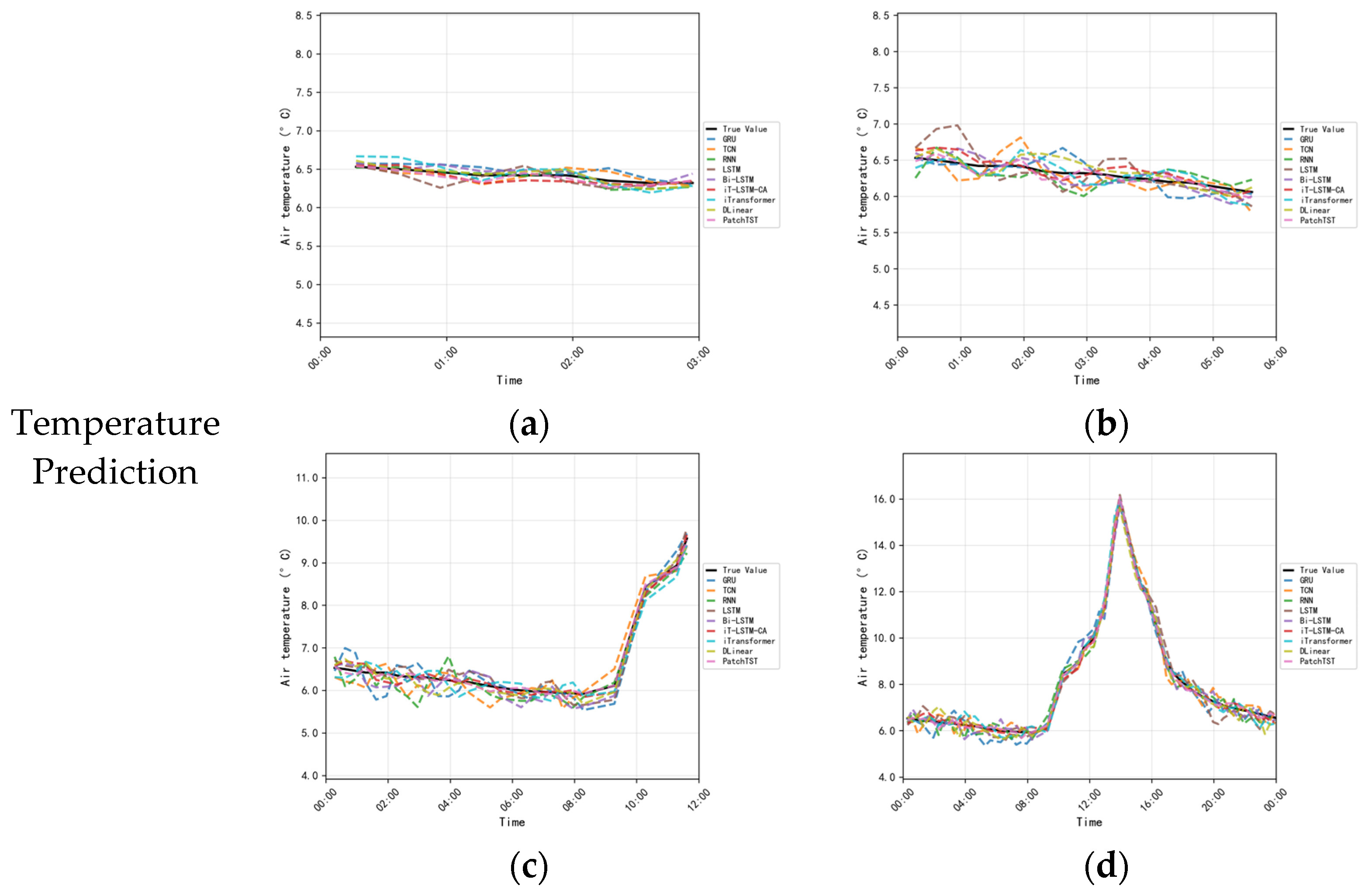
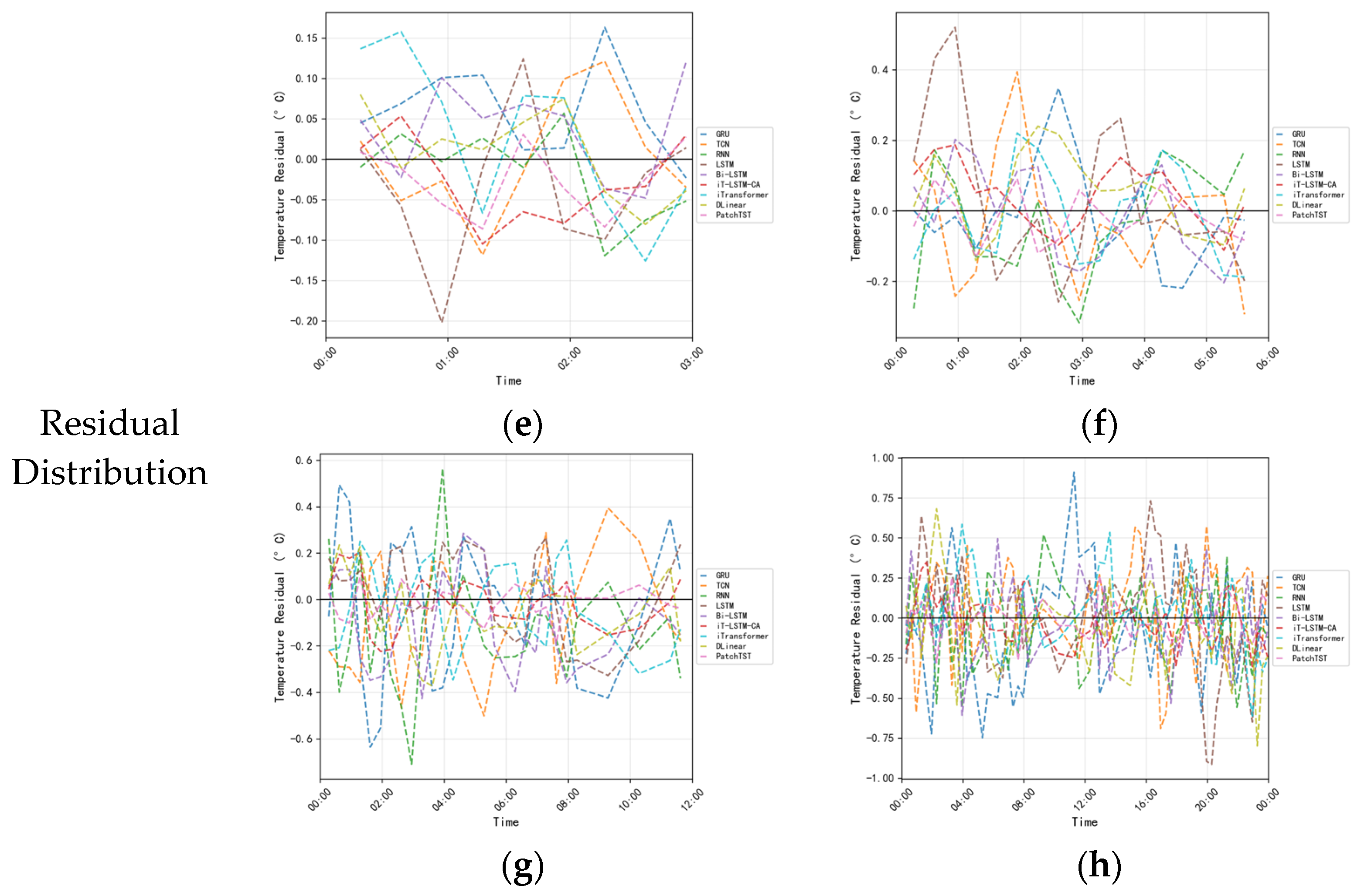
Figure 6 shows the temperature prediction results and the temporal variation of residuals for each model at different prediction horizons. From the prediction curves in Figure 6a–d, it can be observed that the iT-LSTM-CA closely follows the actual temperature fluctuations, with errors remaining within ±0.5 °C for the vast majority of time points. During periods of gradual change, deviations are less than 0.3 °C, while during rapid temperature rises or drops, the maximum error is approximately 0.7 °C. PatchTST captures the overall trend well, but instantaneous errors reach up to 0.9 °C during rapid temperature changes. Residual analysis in Figure 6e–h shows that the iT-LSTM-CA residuals are primarily concentrated between −0.5 °C and 0.5 °C, indicating strong randomness in prediction errors and minimal systematic bias. PatchTST residuals fluctuate roughly between −0.7 °C and 0.6 °C, showing localized deviations during abrupt temperature rises or drops. Traditional models exhibit larger residual fluctuations, with some time points exceeding ±1.0 °C and evident lag effects.

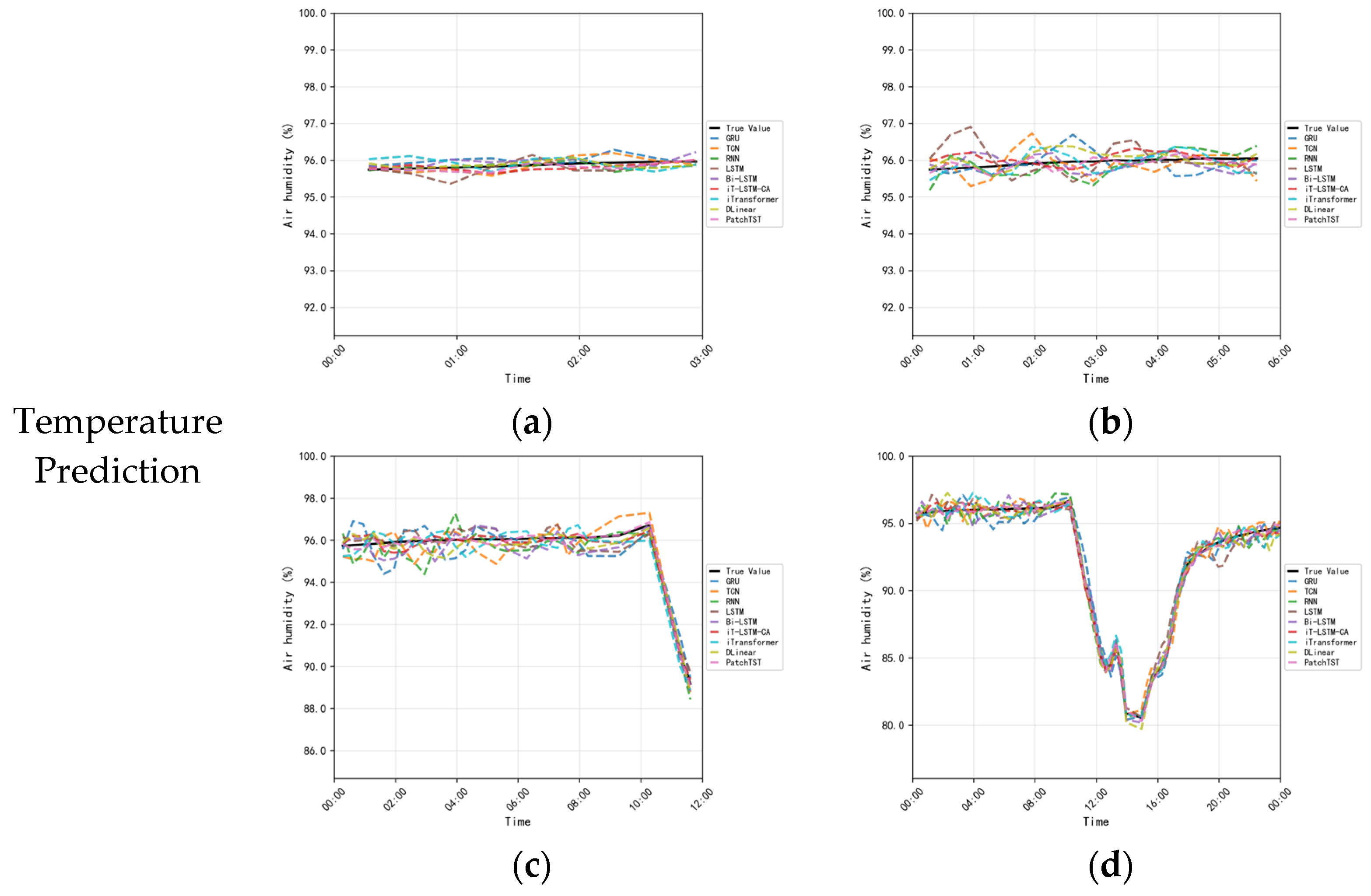
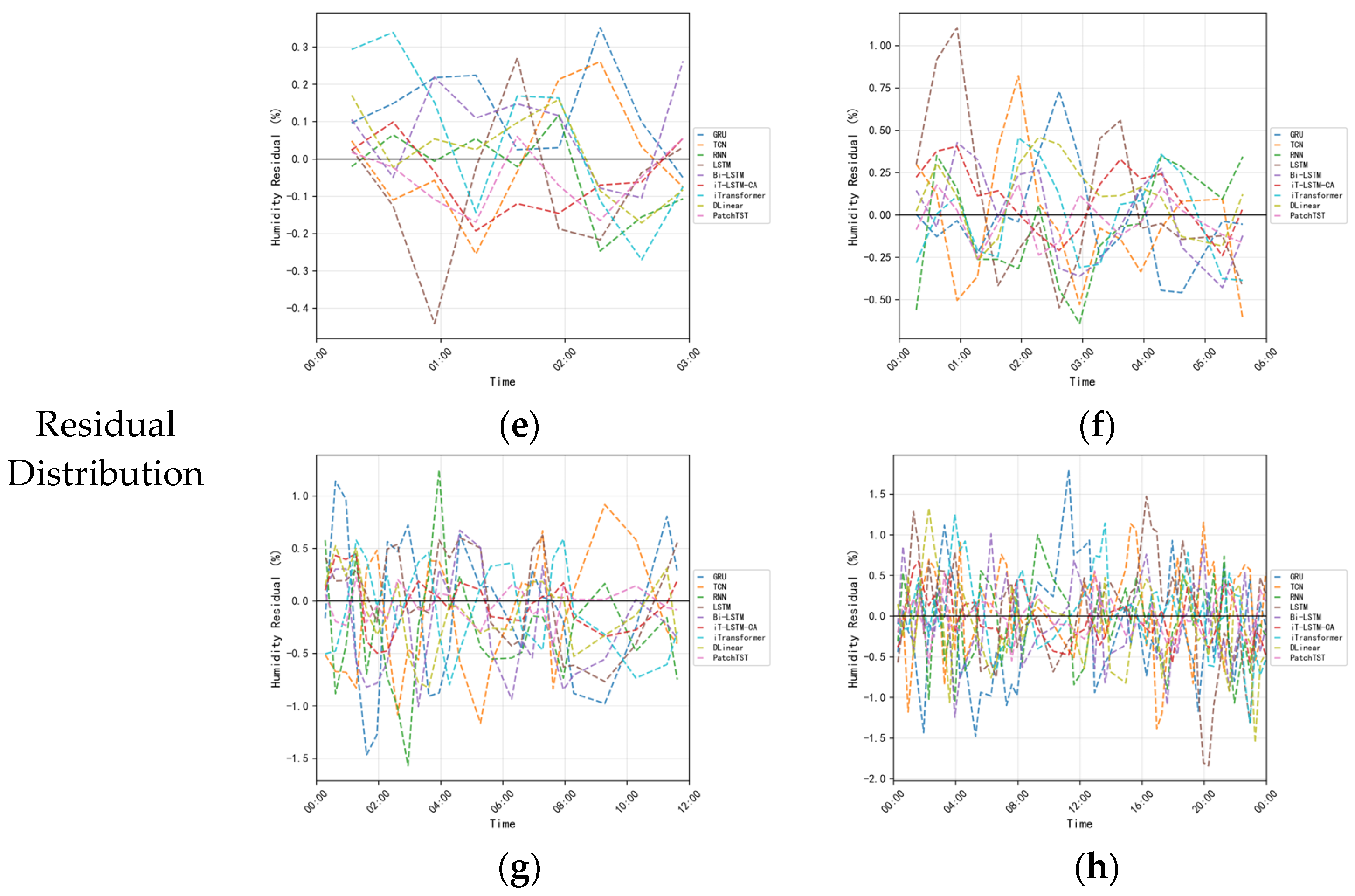
Figure 7 presents the humidity prediction results and the temporal variation of residuals for each model at different prediction horizons. From the prediction curves in Figure 7a–d, the iT-LSTM-CA accurately captures the overall humidity fluctuation trends, maintaining errors within ±1.5% for most time points. During stable humidity periods, deviations are typically below 1%, while during rapid humidity increases or decreases, the maximum error reaches approximately 2.3%. PatchTST remains stable for most periods, but localized errors can reach 2.5% during abrupt changes. Temporal residual analysis shows that the iT-LSTM-CA residuals are mainly concentrated between −1.5% and 1.5%; PatchTST exhibits slightly larger residuals during rapid changes, with a wider fluctuation range; traditional models display more dispersed residuals, with some time points exceeding ±3%, showing noticeable lag and prediction offsets.

3.6. Analysis of Model Prediction Results Under Different Seasons and Weather Conditions

To investigate the stability and adaptability of the iT-LSTM-CA model under varying environmental conditions, a statistical analysis of the model’s predictive performance was conducted along the dimensions of season and weather.

According to the seasonal data in

Table 11. Temperature and Humidity Prediction Results under Different Seasons.

Season	Temperature			Humidity
	MAE/°C	RMSE/°C	R2	MAE/%	RMSE/%	R2
Autumn	0.57 ± 0.02	0.78 ± 0.04	0.97	1.82 ± 0.05	2.63 ± 0.09	0.95
Winter	0.63 ± 0.05	0.85 ± 0.08	0.96	1.94 ± 0.08	2.84 ± 0.12	0.95

, the model demonstrates high prediction accuracy in both autumn and winter. Comparatively, the temperature and humidity prediction errors in autumn are slightly lower than those in winter. Although temperature and humidity fluctuations are larger in winter, leading to a slight increase in MAE, the R² values remain above 0.95. Overall, while seasonal variations can have some impact on temperature and humidity prediction accuracy, the model maintains high R² across different seasons, indicating good stability and adaptability.

From the weather condition data in

Table 12. Temperature and Humidity Prediction Results under Different Weather Conditions.

Weather Condition	Temperature			Humidity
	MAE/°C	RMSE/°C	R2	MAE/%	RMSE/%	R2
Sunny	0.56 ± 0.02	0.74 ± 0.03	0.97	1.78 ± 0.05	2.59 ± 0.08	0.96
Overcast	0.61 ± 0.03	0.82 ± 0.04	0.96	1.92 ± 0.07	2.71 ± 0.10	0.95
Rainy	0.65 ± 0.04	0.86 ± 0.06	0.96	2.11 ± 0.11	2.87 ± 0.14	0.94

, predictions under sunny conditions are the most accurate, while overcast and rainy conditions slightly affect prediction performance. Temperature prediction under rainy conditions is slightly lower than under sunny conditions, with an MAE of 0.65 °C. Humidity prediction is more affected by rapid changes during rain, with an MAE of 2.11%; however, the overall trend of temperature and humidity is still captured accurately, with R² values remaining between 0.94 and 0.96. These results indicate that the model possesses strong environmental adaptability and stability.

4. Discussion and Conclusions

4.1. Discussion

The experimental results of this study demonstrate that, in multivariate environmental prediction tasks for facility-based tomato greenhouses, the introduction of explicit global feature modeling mechanisms plays a critical role in improving multi-step forecasting performance. Compared with traditional single-path time series models, the proposed iT-LSTM-CA model achieves superior overall performance in terms of both prediction accuracy and stability by capturing the synergistic relationship between global trend features and local temporal disturbances. In medium- and long-term forecasting tasks, recurrent neural networks such as LSTM or GRU, which rely solely on implicit modeling of temporal dependencies, struggle to adequately represent the slowly varying trends formed by the combined effects of external meteorological conditions, crop transpiration, and human management operations. In contrast, the iTransformer module introduces an attention mechanism along the variable dimension, enabling explicit modeling of global correlations among environmental factors such as temperature and humidity. This advantage becomes particularly evident in medium- and long-term forecasting horizons, such as 12 h and 24 h. On this basis, the incorporation of a cross-attention mechanism further strengthens the guidance of global trend features over local dynamic variations, allowing the model to maintain high prediction consistency and robustness across different forecasting horizons.

The significance of multi-step environmental prediction lies not only in error reduction but also in its support for refined greenhouse environmental control and optimized resource allocation. High-accuracy temperature and humidity forecasts provide proactive decision support for control actions such as ventilation, shading, heating, and humidification, thereby reducing energy waste caused by delayed regulation or excessive intervention. While ensuring a suitable environment for crop growth, such predictive capabilities enhance greenhouse operational energy efficiency and promote sustainable management. However, the performance of data-driven models largely depends on the continuity and reliability of IoT sensor data. Although the sliding-window median imputation method adopted in this study alleviates the impact of missing data, real-world production environments may still suffer from data quality degradation due to sensor aging, environmental contamination, and communication interruptions, which can adversely affect the long-term stable operation of the model. Therefore, the coordinated design of predictive models with appropriate sensor deployment strategies, periodic calibration, and online anomaly detection and data quality assessment mechanisms represents a key prerequisite for ensuring long-term stable model operation and the sustainable application of greenhouse systems.

4.2. Conclusions

To address the limitations of traditional LSTM models in multivariate environmental prediction for facility-based tomato greenhouses—particularly their insufficient ability to capture global features and the resulting degradation in long-term forecasting accuracy—this study proposes a multi-step prediction model based on iT-LSTM-CA. The global trend features of the greenhouse temperature and humidity sequence are extracted through the iTransformer module. The LSTM module enhances the perception ability of local time series changes. Meanwhile, a cross-attention mechanism is introduced to achieve dynamic fusion of global and local features, thereby improving the accuracy and stability of multi-step prediction. The conclusion is as follows:

(1)

Compared with GRU, TCN, RNN, LSTM, and Bi-LSTM models, iT-LSTM-CA demonstrates lower RMSE and MAE as well as higher R² in multi-step predictions of temperature and humidity, achieving superior predictive performance, providing a reliable data foundation for proactive greenhouse environmental control and stable system operation.

(2)

The prediction curves of the iT-LSTM-CA model closely align with the observed values, accurately reflecting the variation trends of temperature and humidity. Specifically, for temperature prediction over 3 h, 6 h, 12 h, and 24 h multi-step forecasts, R² ranges from 0.96 to 0.98, with a maximum mean absolute error (MAE) of 0.79 °C and a maximum root mean square error (RMSE) of 1.06 °C. For humidity prediction, R² ranges from 0.95 to 0.97, with a maximum MAE of 2.49% and a maximum RMSE of 3.42%. Furthermore, the model’s predictions can provide a scientific basis for the management of facility tomato greenhouse environments, supporting the optimization of ventilation, heating, and humidification strategies, while ensuring crop yield and quality, reducing energy consumption, minimizing resource waste, and promoting facility tomato production toward high efficiency, low consumption, and sustainable development.

4.3. Limitations and Future Work

Although the proposed model demonstrates strong performance in the experiments, several limitations remain. First, in terms of spatiotemporal generalization, the experimental data were collected from a single greenhouse site and were concentrated within a specific growing season. Cross-seasonal and cross-regional multi-site validation has not yet been conducted. Given the variability in regional conditions and the potential impact of seasonal extreme weather events on greenhouse microclimates, the model’s generalization ability under extreme meteorological conditions and over longer time scales still requires further evaluation. Second, regarding model complexity and deployment cost, the introduction of the cross-attention mechanism and the dual-path feature extraction architecture improves prediction accuracy but also increases computational overhead. While the model runs stably on high-performance server platforms, its memory consumption and inference power requirements remain relatively high for resource-constrained greenhouse edge devices. Moreover, lightweight optimization techniques such as pruning and knowledge distillation have not yet been explored, which limits large-scale, low-cost deployment. In addition, the current model is mainly applied at the offline or online prediction stage and has not yet been integrated into a complete closed-loop control system with greenhouse actuators. Consequently, its support for practical production decision-making is still limited to early warning and auxiliary analysis.

To address these limitations, future work will focus on several directions. On the one hand, transfer learning and incremental learning techniques will be introduced, together with multi-site and cross-season datasets and physical prior knowledge, to enhance the robustness and generalization ability of the model under complex environments and extreme weather conditions, providing technical support for the long-term stable operation and risk-adaptive management of greenhouse systems in the context of climate change. On the other hand, lightweight model design and edge-side inference optimization will be explored to reduce computational and energy costs, enabling the sustainable deployment and widespread application of environmental prediction models on low-computing-power, low-energy-consumption devices. Meanwhile, the environmental prediction model will be further integrated with greenhouse control systems to construct a closed-loop regulation framework based on model predictive control (MPC), allowing proactive and optimized control of actuators such as shading screens, ventilation, and supplemental lighting, thereby ensuring crop yield and quality while promoting facility agriculture toward energy-efficient operation, resource-efficient utilization, environmentally friendly practices, and sustainable development.

References

1. Li, Y.; Henke, M.; Zhang, D.; Wang, C.; Wei, M. Optimized Tomato Production in Chinese Solar Greenhouses: The Impact of an East–West Orientation and Wide Row Spacing. Agronomy 2024, 14, 314. [Google Scholar] [CrossRef] [Scilit]
2. Sun, Y.; He, J.; Wei, F.; Yang, W. Development of China’s Tomato Industry during the 13th Five-Year Plan Period and Evaluation of Its International Competitiveness. China Cucurbits Veg. 2023, 36, 112–116. [Google Scholar] [CrossRef]
3. Harel, D.; Fadida, H.; Slepoy, A.; Gantz, S.; Shilo, K. The Effect of Mean Daily Temperature and Relative Humidity on Pollen, Fruit Set and Yield of Tomato Grown in Commercial Protected Cultivation. Agronomy 2014, 4, 167–177. [Google Scholar] [CrossRef] [Scilit]
4. Zheng, Y.; Yang, Z.; Xu, C.; Wang, L.; Huang, H.; Yang, S. The Interactive Effects of Daytime High Temperature and Humidity on Growth and Endogenous Hormone Concentration of Tomato Seedlings. HortScience 2020, 55, 1575–1583. [Google Scholar] [CrossRef] [Scilit]
5. Zero, E.; Sallak, M.; Sacile, R. Predictive Maintenance in IoT-Monitored Systems for Fault Prevention. J. Sens. Actuator Netw. 2024, 13, 57. [Google Scholar] [CrossRef] [Scilit]
6. Varela-Aldás, J.; Gavilanes, A.; Velasco, N.; Del-Valle-Soto, C.; Bran, C. Acceptance of an IoT System for Strawberry Cultivation: A Case Study of Different Users. Sustainability 2024, 16, 7221. [Google Scholar] [CrossRef] [Scilit]
7. Malabadi, R.B.; Kolkar, K.P.; Chalannavar, R.K.; Coronado, K.V.C.; Mammadova, S.S.; Baijnath, H.; Munhoz, A.N.R.; Abdi, G. Greenhouse Farming: Hydroponic Vertical Farming-Internet of Things (IOT) Technologies: An Updated Review. World J. Adv. Res. Rev. 2024, 23, 2634–2686. [Google Scholar] [CrossRef] [Scilit]
8. Ren, S.; Liu, X.; Gu, X.; Wang, H.; Yuan, P.; Xu, H. Multi-Step Rolling Prediction Model of Greenhouse Microclimate Based on R-BP Neural Network. Chin. Agric. Meteorol. 2018, 39, 314–324. [Google Scholar]
9. Francik, S.; Kurpaska, S. The Use of Artificial Neural Networks for Forecasting of Air Temperature inside a Heated Foil Tunnel. Sensors 2020, 20, 652. [Google Scholar] [CrossRef] [Scilit]
10. Liu, Y.; Li, D.; Wan, S.; Wang, F.; Dou, W.; Xu, X.; Li, S.; Ma, R.; Qi, L. A Long Short-term Memory-based Model for Greenhouse Climate Prediction. Int. J. Intell. Syst. 2022, 37, 135–151. [Google Scholar] [CrossRef] [Scilit]
11. Yang, Y.; Gao, P.; Sun, Z.; Wang, H.; Lu, M.; Liu, Y.; Hu, J. Multistep Ahead Prediction of Temperature and Humidity in Solar Greenhouse Based on FAM-LSTM Model. Comput. Electron. Agric. 2023, 213, 108261. [Google Scholar] [CrossRef] [Scilit]
12. Guo, Z.; Feng, L. Multi-Step Prediction of Greenhouse Temperature and Humidity Based on Temporal Position Attention LSTM. Stoch. Environ. Res. Risk Assess. 2024, 38, 4907–4934. [Google Scholar] [CrossRef] [Scilit]
13. Huang, S.; Liu, Q.; Wu, Y.; Chen, M.; Yin, H.; Zhao, J. Edible Mushroom Greenhouse Environment Prediction Model Based on Attention CNN-LSTM. Agronomy 2024, 14, 473. [Google Scholar] [CrossRef] [Scilit]
14. Shi, D.; Yuan, P.; Liang, L.; Gao, L.; Li, M.; Diao, M. Integration of Deep Learning and Sparrow Search Algorithms to Optimize Greenhouse Microclimate Prediction for Seedling Environment Suitability. Agronomy 2024, 14, 254. [Google Scholar] [CrossRef] [Scilit]
15. Zhang, W.; Ren, L.; Wang, F. Research on a Greenhouse Environment Prediction Model Based on an SO-BP Neural Network. J. Chin. Agric. Mech. 2024, 45, 94–99, 106. [Google Scholar] [CrossRef]
16. Liang, Z.; Qi, S.; Chang, Q.; Zhang, P.; Zhang, G.; Niu, L. Greenhouse Environment Prediction Model Based on LSTM–SVM. Trans. Chin. Soc. Agric. Mach. 2025, 56, 279–287. [Google Scholar]
17. Zu, L.; Liu, P.; Zhao, Y.; Li, T.; Li, H. Study on a Greenhouse Environment Prediction Model Based on SSA–LSTM. Trans. Chin. Soc. Agric. Mach. 2023, 54, 351–358. [Google Scholar]
18. Meng, F.; Xu, R.; Zhao, W.; Song, W.; Gao, Y.; Li, L. Sunlight Greenhouse Environment Prediction Model Based on SSA–LSTM–Attention. Trans. Chin. Soc. Agric. Eng. 2025, 41, 256–263. [Google Scholar]
19. Li, X.; Zhang, L.; Wang, X.; Liang, B. Forecasting Greenhouse Air and Soil Temperatures: A Multi-Step Time Series Approach Employing Attention-Based LSTM Network. Comput. Electron. Agric. 2024, 217, 108602. [Google Scholar] [CrossRef] [Scilit]
20. Liu, Y.; Hu, T.; Zhang, H.; Wu, H.; Wang, S.; Ma, L.; Long, M. iTransformer: Inverted Transformers Are Effective for Time Series Forecasting. arXiv 2024, arXiv:2310.06625. [Google Scholar] [CrossRef] [Scilit]
21. Wang, F.; Wang, Y.; Chen, W.; Zhao, C. An Improved iTransformer with RevIN and SSA for Greenhouse Soil Temperature Prediction. Agronomy 2025, 15, 223. [Google Scholar] [CrossRef] [Scilit]
22. Song, C.; Liu, P.; Liu, X.; Yu, Y. Optimization Strategy for Temperature Sensor Deployment in Sunlight Greenhouses Based on HSIC. Trans. Chin. Soc. Agric. Eng. 2022, 38, 200–208. [Google Scholar]
23. Li, Y.; Wang, S.; Chen, Q.; Wang, X. Comparative Study of Several Novel Swarm Intelligence Optimization Algorithms. Comput. Eng. Appl. 2020, 56, 1–12. [Google Scholar] [CrossRef] [Scilit]
24. Xu, Y.; Chen, Z.; Li, T.; Li, C. Time Series Forecasting Based on Seasonally Decomposed Hybrid Neural Networks. Comput. Sci. 2024, 51, 553–559. [Google Scholar]
25. Liu, J.; Zhao, H.; Luo, X.; Xu, Y. Research Progress on Deep Learning Batch Normalization and Related Algorithms. Acta Autom. Sin. 2020, 46, 1090–1120. [Google Scholar] [CrossRef]
26. Hua, Y.; Zhao, Z.; Li, R.; Chen, X.; Liu, Z.; Zhang, H. Deep Learning with Long Short-Term Memory for Time Series Prediction. IEEE Commun. Mag. 2019, 57, 114–119. [Google Scholar] [CrossRef] [Scilit]
27. Liu, J.; Song, Z. A Review of Recurrent Neural Networks. Control Decis. 2022, 37, 2753–2768. [Google Scholar] [CrossRef]
28. Zhong, C.; Zheng, Z. MGGTSP-CAT: Integrating Temporal Convolution and LSTM for Multi-Scale Greenhouse Gas Time Series Prediction via Cross-Attention Mechanism. Adv. Theory Simul. 2024, 7, 2400527. [Google Scholar] [CrossRef] [Scilit]
Figure 1. IoT Data Acquisition System.
Sustainability 18 00930 g001
Figure 2. Comparison diagram before and after data preprocessing (taking indoor temperature and humidity as an example): (a) Temperature Data Preprocessing; (b) Humidity Data Preprocessing.
Sustainability 18 00930 g002
Figure 3. Model architecture of iTransformer: (a) raw series of different variates are independently embedded to tokens; (b) self-attention is applied to embedded variate tokens with enhanced interpretability revealing multivariate correlations; (c) series representations of each token are extracted by the shared feedforward network; (d) layer normalization is adopted to reduce the discrepancies among variates.
Sustainability 18 00930 g003
Figure 4. Model architecture of LSTM.
Sustainability 18 00930 g004
Figure 5. Overall Architecture of the Proposed Model.
Sustainability 18 00930 g005
Figure 6. Comparison of Temperature Prediction Values and True Values by Different Models at Different Prediction Time Lengths: (a) 3 h temperature prediction; (b) 6 h temperature prediction; (c) 12 h temperature prediction; (d) 24 h temperature prediction; (e) 3 h residual distribution; (f) 6 h residual distribution; (g) 12 h residual distribution; (h) 24 h residual distribution.
Sustainability 18 00930 g006aSustainability 18 00930 g006b
Figure 7. Comparison of Humidity Prediction Values and True Values by Different Models at Different Prediction Time Lengths: (a) 3 h humidity prediction; (b) 6 h humidity prediction; (c) 12 h humidity prediction; (d) 24 h humidity prediction; (e) 3 h residual distribution; (f) 6 h residual distribution; (g) 12 h residual distribution; (h) 24 h residual distribution.
Sustainability 18 00930 g007aSustainability 18 00930 g007b