Decarbonizing Coastal Shipping: Voyage-Level CO₂ Intensity, Fuel Switching and Carbon Pricing in a Distribution-Free Causal Framework

Abstract

Coastal shipping plays a critical role in meeting maritime decarbonization targets under the International Maritime Organization’s (IMO) Carbon Intensity Indicator (CII) and the European Union Emissions Trading System (EU ETS); however, operators currently lack robust tools to forecast route-specific carbon intensity and evaluate the causal benefits of fuel switching. This study developed a distribution-free causal forecasting framework for voyage-level Carbon Dioxide (CO₂) intensity using an enriched panel of 1440 real-world voyages across four Nigerian coastal routes (2022–2024). We employed a physics-informed monotonic Light Gradient Boosting Machine (LightGBM) model trained under a strict leave-one-route-out (LORO) protocol, integrated with split-conformal prediction for uncertainty quantification and Causal Forests for estimating heterogeneous treatment effects. The model predicted emission intensity on completely unseen corridors with a Mean Absolute Error (MAE) of 40.7 kg CO₂/nm, while 90% conformal prediction intervals achieved 100% empirical coverage. While the global average effect of switching from heavy fuel oil to diesel was negligible (≈−0.07 kg CO₂/nm), Causal Forests revealed significant heterogeneity, with effects ranging from −74 g to +29 g CO₂/nm depending on route conditions. Economically, targeted diesel use becomes viable only when carbon prices exceed ~100 USD/tCO₂. These findings demonstrate that effective coastal decarbonization requires moving beyond static baselines to uncertainty-aware planning and targeted, route-specific fuel strategies rather than uniform fleet-wide policies.

1. Introduction

The international maritime sector is undergoing a regulatory transformation. The International Maritime Organization (IMO) introduced the Carbon Intensity Indicator (CII) in 2023 as a mandatory operational rating scheme aimed at reducing greenhouse gas emissions from international shipping by at least 40% by 2030 compared to 2008 levels [1,2,3]. The CII grades vessels from A to E are based on annual CO₂ per ton-nautical mile, with corrective action required for persistent D/E performance [1,2,4]. Non-compliance can lead to detention, fines, and loss of market access [5,6]. In parallel, the EU ETS extension to shipping and FuelEU Maritime are expected to impose carbon prices of several tens to about one hundred USD/tCO₂ [2,7,8,9]. Together, these regimes require methods that forecast voyage-level emission intensity and credibly evaluate operational measures [10]. Even small efficiency gains reduce fuel and CO₂ [11], and fuel choice—including cleaner alternatives to HFO—has become a key lever [12].

Maritime decarbonization supports the Sustainable Development Goals, notably Sustainable Development Goals (SDG) 13, SDG 9, and SDG 14 [13,14]. Because coastal and short-sea shipping connect hubs and communities, their emissions directly affect development and marine ecosystems [15], and coastal corridors can serve as practical testbeds where route-specific decision tools help align IMO measures with the Paris goals [16,17]. Achieving net-zero shipping by mid-century will require coupling operational improvements with high-level policy instruments (including coordinated carbon-pricing frameworks) and technology pathways such as alternative fuels and green-corridor deployment [18]. Consistent with the expert review-based agenda articulated by Govindan et al. [18], priority gaps include rigorous cost–benefit evaluation of port initiatives, the investment and techno-economic feasibility of onboard carbon capture and alternative fuels (with green shipping corridors as an adoption catalyst), and the design of carbon pricing under intertwined climate, economic, and socio-political constraints in ongoing IMO negotiations and in regional schemes such as the EU ETS [18]. Within this broader transition, our route- and season-specific risk and causal evidence provide an implementation-layer input for designing fair and effective corridor strategies. Near-coastal decarbonization is not a ship-only problem: emissions outcomes on short-sea corridors are shaped by port energy infrastructure, electrification of port-side services, and the availability of cleaner fuels and shore power; smart-port studies highlight ISO 50001-aligned energy management and digital monitoring as practical levers for reducing Greenhouse Gas (GHG) emissions and improving operational control [2], while complementary work emphasizes shore power (“cold ironing”) and port-side renewables as mitigation options for coastal networks [5]. Recent scoping evidence on renewable-powered seaport operations highlights the growing role of port Energy Management Systems and integrated renewables (e.g., solar, wind, and marine energy) in reducing seaport carbon footprints and enabling greener coastal logistics [19]. However, measure effectiveness is mixed, and switching from heavy fuel oil (HFO) to marine diesel oil (MDO) can be heavily confounded by operating conditions [20,21]; fuel use and carbon intensity respond nonlinearly to speed, draft, weather and hull condition, and coastal trades add shallow-water effects and maneuvering [22]. Naïve comparisons can therefore bias estimated switching benefits [21]. Causal methods are needed to isolate fuel effects, and findings should be interpreted alongside Energy Efficiency Design Index (EEDI) and Ship Energy Efficiency Management Plan (SEEMP) [23,24,25,26]; because fuel and routing choices have externalities, causal evidence can also support targeted governance interventions [27,28,29].

Machine learning (ML) adoption in maritime energy-efficiency modelling has accelerated [8]. Models such as neural networks and gradient boosting can predict fuel consumption and emission intensity within familiar operating envelopes, but most studies evaluate performance in-distribution rather than with route-wise holdout such as leave-one-route-out [11,30]. The harder regulatory problem is forecasting on unseen routes under distribution shift, where covariate distributions deviate from training and point accuracy can be misleading; classical regression-based confidence intervals also break down on heavy-tailed, multimodal voyage data [31]. Conformal prediction offers distribution-free intervals with finite-sample coverage guarantees [32]. Such robustness matters as targets tighten and operators need to separate weather-driven variability from decision-driven effects in energy-efficiency indicators [12,33]. Uncertainty-aware forecasting is therefore central to compliance and risk reporting rather than a purely technical add-on [2] because under-estimating emissions can trigger penalties and over-estimating can lead to unnecessary costs.

A further challenge is that many operational datasets omit deadweight tonnage (DWT), which is required for official CII computation [34]. In practice, operators often rely on transport-work-agnostic targets such as voyage-level CI (kg CO₂/nm), but modeling pipelines should remain explicitly “CII ready” so the target can later be swapped to Annual Efficiency Ratio (AER)/CII when design parameters become available [2,35]. Because intensity metrics influence sustainable-finance signals and carbon-pricing credibility, unstable measures can distort incentives and reporting [36,37]. This risk is amplified when charges or performance thresholds hinge on unobserved factors [37]. Architectures compatible with current indicators and future CII/AER metrics therefore support a smoother transition [38]. Recent work on maritime decarbonization and operational analytics has advanced emissions forecasting and compliance-oriented indicators, but it is still largely evaluated under in-distribution settings and with limited deployment realism for new corridors [10,11]. In parallel, empirical assessments of operational measures (including fuel switching) often remain associational, making estimates sensitive to route- and condition-driven confounding [21,23]. These considerations expose three gaps: unseen-route generalization, distribution-free uncertainty, and causal identification of fuel-switching effects under confounding [21,39].

Existing ML-based maritime emissions studies typically prioritize point prediction accuracy under random or in-distribution train–test splits and rarely test deployment on entirely new corridors where covariate distributions shift [10,11]. In parallel, uncertainty is often omitted or approximated with parametric confidence intervals whose assumptions are brittle in heavy-tailed voyage data and under route-wise domain shift [31]. Moreover, empirical assessments of operational measures such as fuel switching frequently remain correlational, so estimated benefits can be confounded by endogenous speed, loading, and routing decisions [21,22,23]. In contrast, we propose a unified pipeline that combines leave-one-route-out evaluation for unseen-route generalization, distribution-free conformal prediction intervals for finite-sample risk quantification [32,40] and causal estimation (Double/Debiased Machine Learning and Causal Forests) for heterogeneous fuel-switching effects [41,42]. These outputs are further operationalized into an exceedance-risk map and Total Cost Intensity analysis under carbon pricing, providing decision-relevant evidence for corridor-level decarbonization planning [2,7].

From a sustainability and governance standpoint, these gaps translate into practical blind spots. Without tools that generalize to new corridors and quantify risk under deep uncertainty, operators cannot reliably plan compliance margins, and regulators cannot distinguish genuine efficiency improvements from statistical artifacts. Likewise, without causal identification, fuel-switching policies may be rewarded or penalized for the wrong reasons, leading to misallocated investment and distorted signals under carbon pricing. Addressing all three gaps together is therefore essential for decision support that is both operationally useful and policy credible. This is particularly acute in coastal services, where corridors change, operating regimes shift quickly, and data constraints are common.

We analyzed 1440 voyages across four Nigerian coastal routes (2022–2024) from a single operator’s noon-reports and Automatic Identification System (AIS) records, released as a public ship fuel-efficiency dataset on Kaggle [43]. From this base, we built a voyage-level panel and model emission intensity as CI (kg CO₂/nm) using engineered operational, environmental, and cost covariates that capture speed and distance effects, route context, weather proxies, and maneuvering conditions. CI is forecast with a physics-informed monotonic LightGBM model under a strict leave-one-route-out protocol; split conformal prediction yields finite-sample intervals on unseen routes; and HFO-to-diesel effects are estimated with Double/Debiased Machine Learning and Causal Forests [41,42]. We then operationalize uncertainty via an Emission Intensity Exceedance Risk metric and integrate Total Cost Intensity (TCI) under alternative carbon prices to support route- and season-specific decisions.

Study design and research questions. This study is an observational, retrospective voyage-level panel analysis of Nigerian short-sea coastal operations (N = 1440 voyages across four routes, 2022–2024) that integrates (i) unseen-route emissions forecasting, (ii) distribution-free uncertainty quantification, and (iii) causal estimation of HFO-to-diesel switching effects under operational confounding. We address three pre-specified research questions:

• RQ1 (Forecasting): Can voyage-level CO₂ intensity be predicted on completely unseen coastal routes under a strict leave-one-route-out design?
• RQ2 (Uncertainty): Can we provide distribution-free prediction intervals with valid coverage on unseen routes to support uncertainty-aware compliance and planning decisions?
• RQ3 (Causal fuel switching): What is the causal effect of switching from HFO to diesel on emission intensity, and how heterogeneous is this effect across route–season operating conditions?

The study makes four contributions. (1) Unseen-route emission forecasting: a physics-informed monotonic LightGBM model with leave-one-route-out training delivers robust predictions on unseen coastal corridors while preserving hydrodynamic monotonicities. (2) Distribution-free risk quantification: split conformal prediction provides 90% prediction intervals with finite-sample guarantees and yields an Emission Intensity Exceedance Risk metric for decision support. (3) Causal assessment of fuel switching: Double/Debiased Machine Learning and Causal Forests show a near-zero average HFO-to-diesel effect but substantial route–season heterogeneity. (4) Economic integration via TCI: emissions outcomes are linked to Total Cost Intensity under alternative carbon prices, clarifying when selective diesel adoption becomes cost-effective. Taken together, the framework provides a practically implementable toolkit for fleet managers and regulators to forecast emissions, quantify compliance risk, and evaluate operational measures in a route- and season-specific way.

The rest of this paper is organized as follows. Section 2 presents the materials and methods, including data construction, descriptive context, and the predictive, uncertainty-quantification, and causal components of the proposed pipeline. Section 3 reports empirical results on unseen-route forecasting performance, uncertainty coverage, causal fuel-switching effects (including heterogeneity), and cost implications under carbon pricing. Section 4 discusses interpretation, policy and operational implications, and limitations. Section 5 concludes with practical recommendations and directions for future work.

2. Materials and Methods

All computations were performed in Python (v3.12.11; Python Software Foundation, Wilmington, DE, USA). Model training and forecasting were conducted using LightGBM (v4.6.0) and scikit-learn (v1.6.1). Model interpretability analyses were carried out using SHAP (v0.48.0). Figures and visualizations were generated using Matplotlib (v3.10.3). Causal estimation, including Double/Debiased Machine Learning (DML) and Causal Forests for heterogeneous treatment effects, was implemented using EconML (v0.16.0).

Methods overview. Our workflow proceeds in four steps. First, we constructed an enriched voyage-level panel from operational noon reports and AIS records and defined voyage-level CO₂ intensity per nautical mile (CI, kg CO₂/nm) as the primary outcome. Second, we trained a physics-informed monotonic LightGBM model under a strict leave-one-route-out (LORO) design to evaluate deployment on completely unseen coastal corridors. Third, we wrapped point forecasts with split conformal inference to obtain distribution-free prediction intervals with finite-sample coverage on unseen routes. Fourth, we estimated the causal effect of switching from HFO to diesel using Double/Debiased Machine Learning Average Treatment Effect (ATE) and Causal Forests heterogeneous Conditional Average Treatment Effect (CATE), relying on overlap/common support diagnostics to support causal interpretation under observed confounding. Finally, we operationalized outputs for decision support through uncertainty-aware risk screening and cost-intensity concepts under carbon pricing scenarios.

Mapping from research questions to methods:

RQ1 → Monotonic LightGBM forecasting under LORO evaluation.

RQ2 → Split conformal prediction intervals and empirical coverage assessment under LORO.

RQ3 → Double/Debiased Machine Learning (DML) for ATE and Causal Forests for heterogeneous CATE, supported by overlap/propensity diagnostics.

2.1. Data Source, Study Setting, and Voyage Panel Construction

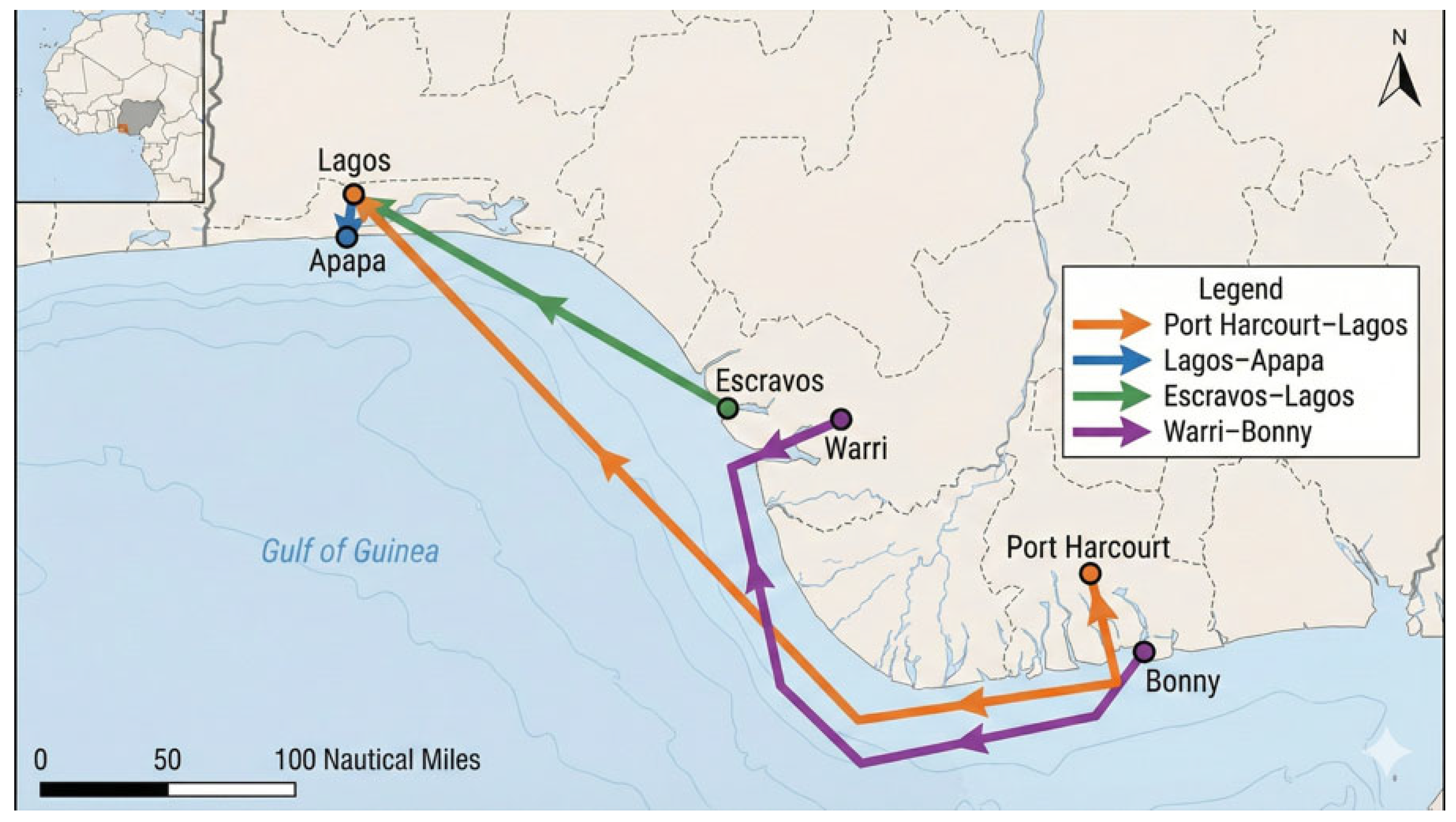
This study analyzed a single-operator panel of 1440 completed coastal voyages performed by general cargo and coastal tanker vessels across four Nigerian short-sea routes (Port Harcourt–Lagos, Lagos–Apapa, Escravos–Lagos, and Warri–Bonny) over the period of January 2022 to December 2024.

Figure 1 summarizes the Nigerian coastal study network, showing the four analyzed routes and their associated ports.

The underlying observations originated from the operator’s standard operational reporting system, combining daily noon reports (fuel logs, engine settings, and operational notes) with Automatic Identification System (AIS) records that provide position and speed-over-ground information. Prior to public release, the data owner anonymized and aggregated these operational records and made them available as the “Ship Fuel Efficiency—Kaggle” dataset [43].

In the present work, the Kaggle dataset was used as the operational starting point, and the modeling dataset was constructed as an enriched voyage-level panel. Specifically, we retained the full set of 1440 real-world Nigerian coastal voyages and derived additional variables tailored to corridor-level short-sea operations and the methodological requirements of unseen-route forecasting and causal inference. These engineered variables included route-relative difficulty metrics (e.g., route_difficulty_score), deviation-based indicators (route_median_ratio and intensity_gap), and season- or weather-normalized emission-intensity measures that support both predictive modeling and treatment-effect estimation. The resulting dataset represents a coherent operational environment in the Gulf of Guinea characterized by homogeneous reporting conventions and a shared commercial context. Additional documentation of the source dataset and the derived voyage-level panel is provided in Appendix A and Appendix B.

2.2. Variables, Definitions, and Preprocessing

The voyage-level panel includes route and time identifiers (route_id, month, season_bin), operational variables (distance_nm, fuel_type, fuel_consumption), environmental conditions (weather_category), outcomes (CO₂ emissions, CI_kg_per_nm), cost variables (energy_cost and carbon-cost components), and engineered route-relative features (route_difficulty_score, route_median_ratio, intensity_gap). Appendix A and Appendix B provide the complete variable dictionaries and construction steps for both the original and derived datasets.

The main variable groups used in the analyses were:

(i)

Route and time: route identifiers (route_id), seasonal bins (season_bin: Winter, Spring, Summer, Autumn), and cyclic temporal encodings that capture intra-annual variation in operating conditions.

(ii)

Operational conditions: voyage distance in nautical miles (distance_nm) and fuel type $(fuel\_type\in HFO,Diesel).$

(iii)

Environmental factors: discrete weather states (weather_category ∈ {Calm, Moderate, Stormy}), constructed from Beaufort-scale logs and significant wave height (Hs) consistent with the operator’s internal reporting conventions for coastal voyages in the Gulf of Guinea.

Table 1. Operational weather categorization criteria.

Category	Beaufort Range	Approx. Hs (m)	Operational Meaning
Calm	0–3	<1.25	Normal coastal steaming, negligible impact on speed.
Moderate	4–5	1.25–2.5	Increased resistance, occasional slamming, minor speed reductions.
Stormy	≥6	>2.5	Heavy-weather maneuvering, enforced speed reductions.

summarizes the classification thresholds.

(iv)

Outcomes and cost drivers: voyage-level fuel consumption, total CO₂ emissions, and energy cost. Carbon-cost components and Total Cost Intensity (TCI) measures were derived for the scenario-based economic analysis and reported in the Section 3.

Primary outcome. The target variable is Voyage-Level Emission Intensity (CI), defined as total CO₂ emissions per nautical mile:

$$CI={\displaystyle \frac{Total {CO}_2 Emissions \left(\mathrm{kg}\right)}{Distance \left(\mathrm{nm}\right)}}$$

(1)

and reported throughout in kg CO₂/nm. Deadweight tonnage (DWT) is unavailable in the dataset, preventing direct computation of official CII in g CO₂/(dwt·nm). While the IMO’s CII is transport-work-based, CI expressed in kg CO₂/nm is widely used in coastal shuttle operations where repeated legs and narrower load variation make per-distance performance monitoring operationally meaningful. Importantly, the modeling pipeline was designed to remain “CII-ready”: once DWT or cargo-mass data become available, the same statistical architecture (feature engineering, prediction, uncertainty quantification, and causal adjustment) can be applied to AER/CII-type outcomes without changing the methodological core.

Preprocessing and data quality. All variables were derived from the operator’s noon-report and AIS workflow. Noon reports are compiled by deck officers once per day or at key voyage stages and include manually entered fuel, weather, and engine settings; AIS provides positional and speed information. As in most operational datasets, occasional inconsistencies and outliers cannot be ruled out. We therefore applied basic plausibility checks and range filters prior to analysis and relied on modeling choices that are robust to residual measurement noise. Load condition (ballast versus laden) was not directly observed; its influence is partially absorbed through route, distance, and seasonal indicators, but transport work was not reconstructed from the available fields.

2.3. Descriptive Statistics and Operational Context

Table 2. Summary statistics of key voyage-level variables (N = 1440). Energy cost reflects bunker expenditure only.

Variable	Mean	Median	Std. Dev.	Min	Max
Distance (nm)	151.8	123.5	108.5	20.1	498.6
Emission Intensity (kg CO2/nm)	78.9	79.2	28.0	25.6	146.6
Total CO2 Emissions (tons)	13.4	8.4	13.6	0.6	71.9
Energy Cost (USD)	2429	1501	2522	142	14,666

summarizes key continuous voyage-level variables (N = 1440). Voyage distances ranged from 20.1 to 498.6 nm (mean 151.8; median 123.5 nm), reflecting fixed-route coastal shuttle operations. The mean emission intensity was 78.9 kg CO₂/nm (median 79.2 kg CO₂/nm), indicating a stable intensity envelope despite substantial heterogeneity in distance and weather exposure. Total CO₂ emissions per voyage ranged from 0.6 to 71.9 tons (mean 13.4; median 8.4 tons). Voyage-level energy cost (bunker expenditure only) ranged from 142 to 14,666 USD (mean 2429; median 1501 USD).

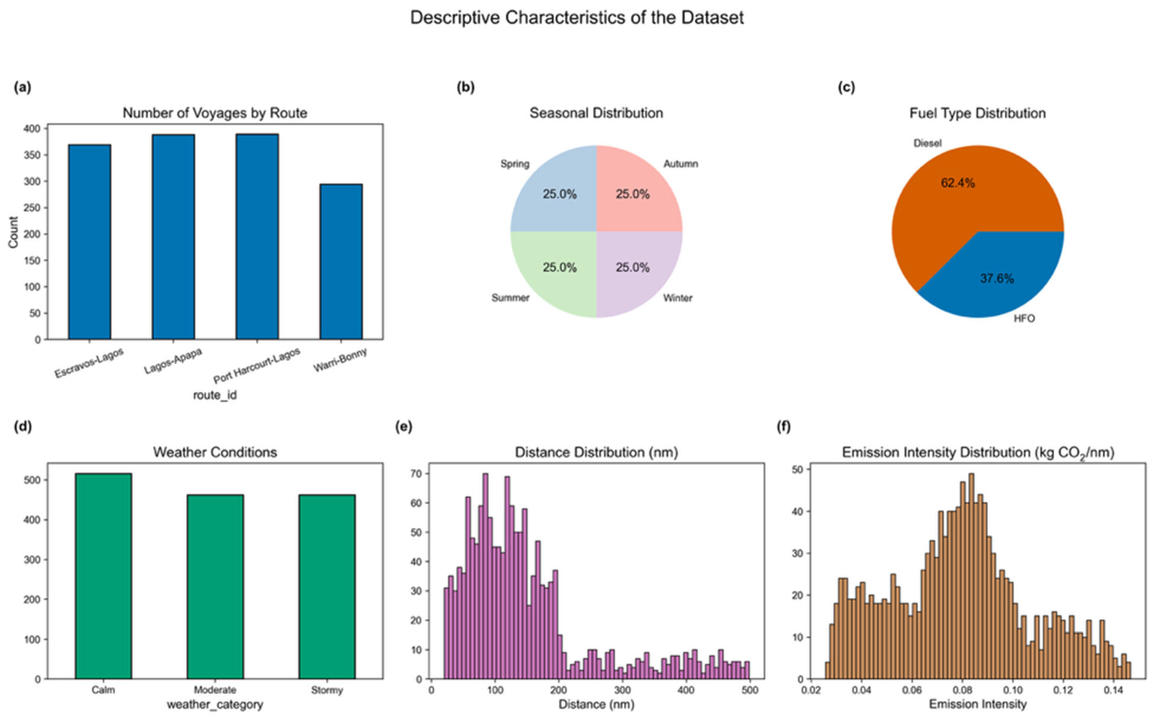
Figure 2 provides an overview of the dataset structure, including route frequencies, seasonal balance (25% per season), fuel shares (Diesel 62.4%, HFO 37.6%), weather distribution (Calm 35.8%, Moderate 32.1%, Stormy 32.1%), and the distance and CI distributions. Operationally, the vessels follow repeated shuttle patterns connecting refinery terminals, river ports, and offshore loading/discharging areas, which implies frequent transitions between open-coast steaming and constrained channel approaches. The four corridors differ in navigational and environmental difficulty: Port Harcourt–Lagos is the longest and involves exposure to bar crossings, offshore currents, and dense traffic; Lagos–Apapa is a very short intra-port leg dominated by low-speed maneuvering and hoteling; Escravos–Lagos and Warri–Bonny involve river-mouth transits and shallow, constrained fairways that increase sensitivity to weather and operational constraints. These corridor characteristics motivate both route-aware predictive evaluation and confounding-aware causal estimation.

2.4. Evidence of Operational Confounding

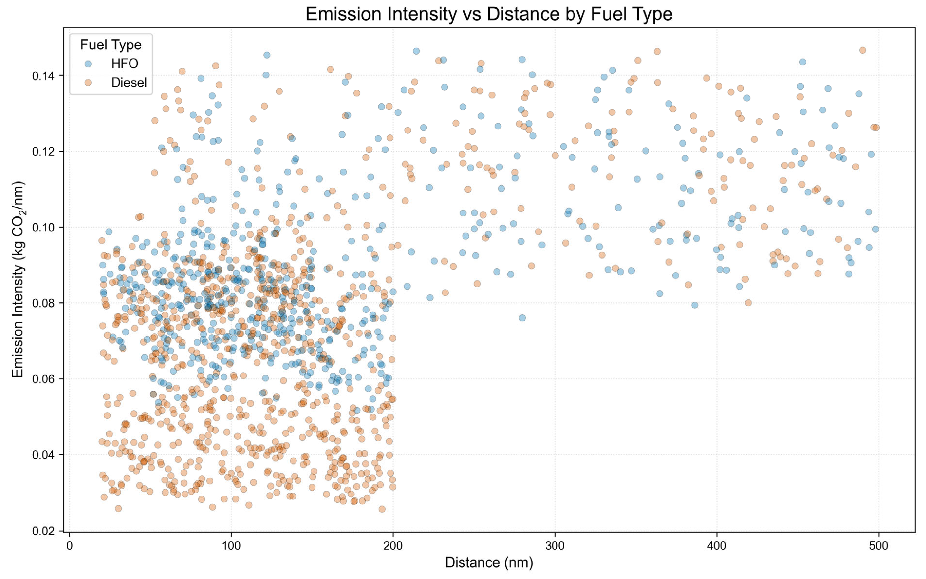
Figure 3 visualizes emission intensity (CI) versus voyage distance, colored by fuel type. A pronounced negative relationship can be observed: longer voyages typically have a higher share of steady cruising relative to maneuvering and port approaches, leading to lower CI. At short distances—typical of intra-port legs such as Lagos–Apapa—CI is elevated because a substantial share of fuel is consumed in low-speed maneuvers, acceleration–deceleration cycles, and hoteling in confined waters. Although Diesel voyages often exhibit lower CI than HFO voyages, there is substantial overlap between fuels across distances, seasons, and weather states. This overlap indicates that fuel choice is endogenous to operational context: naïve comparisons that ignore distance, route geometry, shallow-water constraints, and weather would yield biased estimates of “fuel switching” benefits. Accordingly, the causal component of our framework explicitly conditions on these covariates and route-relative metrics when estimating the effect of switching from HFO to Diesel.

2.5. Predictive Modeling for Unseen Routes

The forecasting task is to predict voyage-level emission intensity on a completely unseen coastal corridor without retraining, reflecting a deployment-realistic scenario for route-specific compliance planning. We used a Light Gradient Boosting Machine (LightGBM) regressor [44] due to its strong performance on heterogeneous tabular data and its ability to capture nonlinear interactions. Categorical identifiers (e.g., ship_id and route_id) are treated as categorical features so that the model can learn vessel- and corridor-associated patterns without requiring manual encoding.

Leakage-free feature engineering. To generalize to unseen routes, route-level statistics must be constructed without leaking information from the held-out corridor. Naively including route means or medians computed on the full dataset would allow the model to implicitly “recognize” the test route. We therefore implemented a strict out-of-fold feature engineering protocol aligned with leave-one-route-out validation. For each fold, one route is held out entirely; all group-derived summaries are computed only on the remaining routes and then projected to voyage level as relative metrics. Key engineered features include route_median_ratio, route_difficulty_score, and intensity_gap, which summarize operational difficulty as deviations from appropriate baselines rather than absolute route identifiers. To explicitly capture operational stress, these features are constructed as relative deviations. Specifically, route_median_ratio is computed as the ratio of a voyage’s emission intensity to the route-specific median (e.g., a ratio of 1.2 indicates an intensity 20% higher than the corridor norm, likely due to weather or maneuvering). The route_difficulty_score represents the absolute deviation from the route mean $(C{I}_{\left\{voyage\right\}}- {\mu }_{\left\{route\right\}})$, retaining the magnitude of intensity spikes, while the intensity_gap measures the deviation from the season-specific median, isolating weather-driven anomalies from baseline seasonal trends. These relative metrics allow the model to learn ‘how difficult’ a voyage is compared to its peers, ensuring that predictions rely on transferable physical signals rather than static route identifiers.

Physics-informed monotonicity. To embed domain knowledge, we imposed a monotonicity constraint on distance_nm, requiring predicted CI to be a non-increasing function of distance (monotone constraint = −1). In coastal shuttle operations, longer voyages tend to allocate more time to efficient cruising and less to fuel-intensive maneuvering and hoteling; thus, CI should not increase with distance, all else being equal. Other covariates (weather, season, route-relative metrics) remained unconstrained to allow for nonlinear interactions.

Hyperparameter configuration. The LightGBM model was configured with $n\_estimators = 2000$, $learning\_rate = 0.01$, $max\_depth = 12$, and $min\_child\_samples = 20$, with remaining parameters set to defaults unless otherwise stated. This configuration balances capacity and regularization to improve robustness under corridor-level distribution shifts.

Unseen-route evaluation (LORO). We evaluated predictive performance under a strict leave-one-route-out (LORO) protocol: in each fold, one corridor is held out as the test set, while the remaining routes are used for leakage-free feature engineering, model fitting, and uncertainty calibration. Performance metrics (MAE, Root Mean Square Error (RMSE), and R²) are computed on the held-out route only and aggregated across folds.

2.6. Distribution-Free Uncertainty Quantification

Point forecasts alone are insufficient for regulatory risk management; decision-makers require uncertainty ranges that remain valid under distribution shifts across corridors. Classical confidence intervals rely on assumptions (e.g., normality and homoscedasticity of residuals) that are often violated in heavy-tailed, multimodal operational voyage data. We therefore constructed distribution-free prediction intervals using split-conformal prediction, which provides finite-sample coverage guarantees [32,40].

Let f(X) denote the fitted LightGBM predictor. Within the LORO framework, absolute residuals are computed on each held-out route as:

$$R_i=\left|Y_i-f\left(X_i\right)\right|,$$

(2)

where Yi is the observed emission intensity for voyage i. Residuals from all folds are pooled into a calibration set {Ri}i = 1 … N to characterize prediction error on unseen corridors. For a target coverage level 1 − α = 0.90, we compute the empirical (1 − α)-quantile $\widehat{q}$ of the pooled residuals. For a new voyage with covariates Xnew on a previously unseen route, the split-conformal prediction interval is:

$$C\left(X_{new}\right)=\left[f\left(X_{\mathrm{new}}\right)-\hat{q},f\left(X_{\mathrm{new}}\right)+\hat{q}\right],$$

(3)

Under exchangeability within the operational domain, this construction guarantees that the true emission intensity Ynew lies within the interval with probability at least 90%, regardless of the underlying noise distribution. In practice, pooling residuals across folds yields conservative intervals because the calibration incorporates worst-case errors observed on challenging corridors, reducing the risk of underestimation in compliance-oriented settings.

2.7. Causal Inference for Fuel Switching

Beyond forecasting and uncertainty, operational and policy decisions require causal evidence: under comparable conditions, when does switching from HFO to Diesel reduce emission intensity, and when does it increase it? We estimated causal effects in a potential outcomes framework. Let T be a binary treatment indicator with $T = 1$ for Diesel and $T=0$ for HFO, and let Y denote observed emission intensity (CI, kg CO₂/nm). Each voyage has potential outcomes Y(1) and Y(0), corresponding to the emission intensity that would be observed under Diesel or HFO, respectively. The primary estimands are the Average Treatment Effect (ATE, defined as the arithmetic mean difference) and Conditional Average Treatment Effects (CATE, defined as the conditional arithmetic mean of the treatment effect) of Diesel relative to HFO.

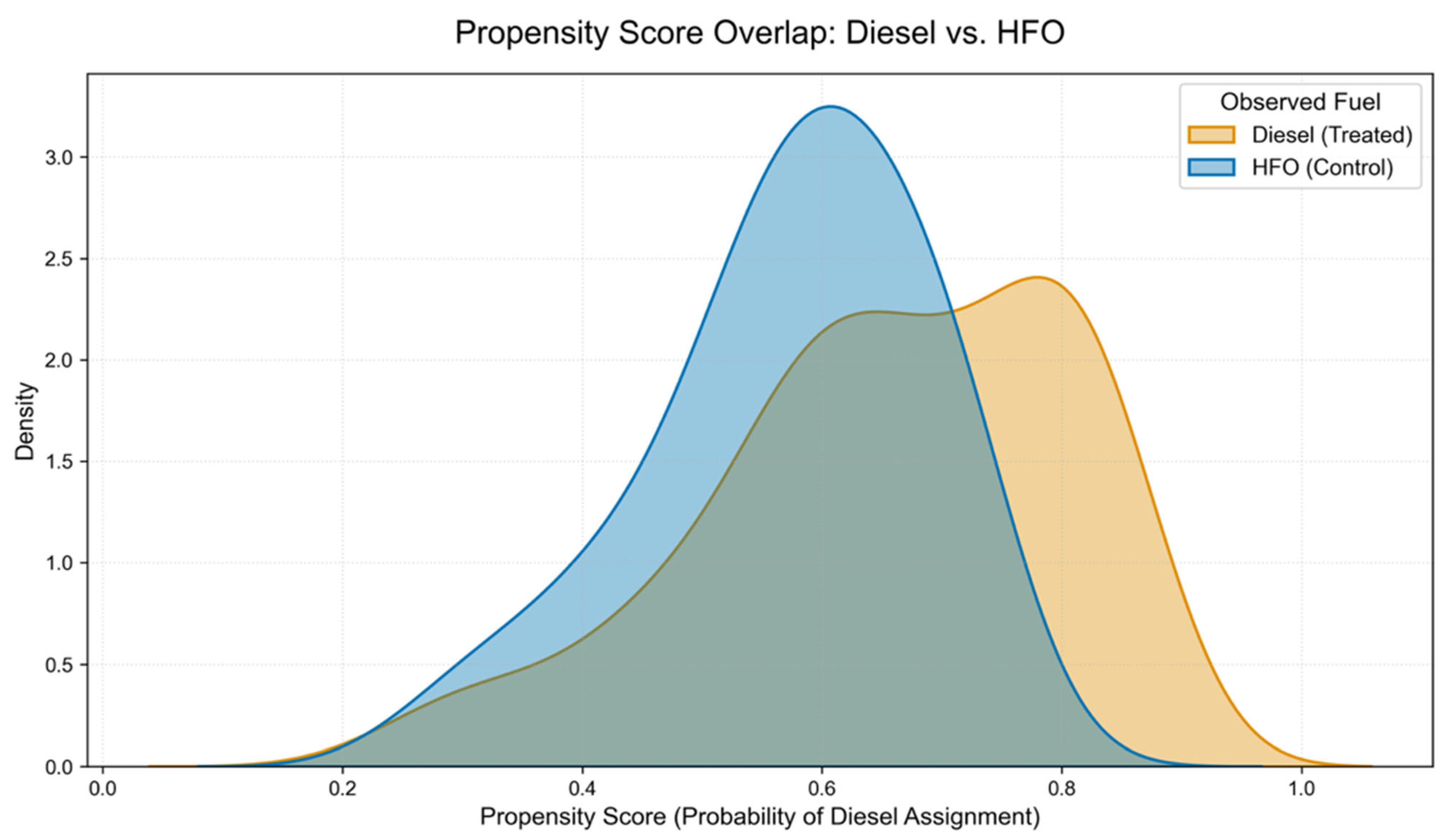
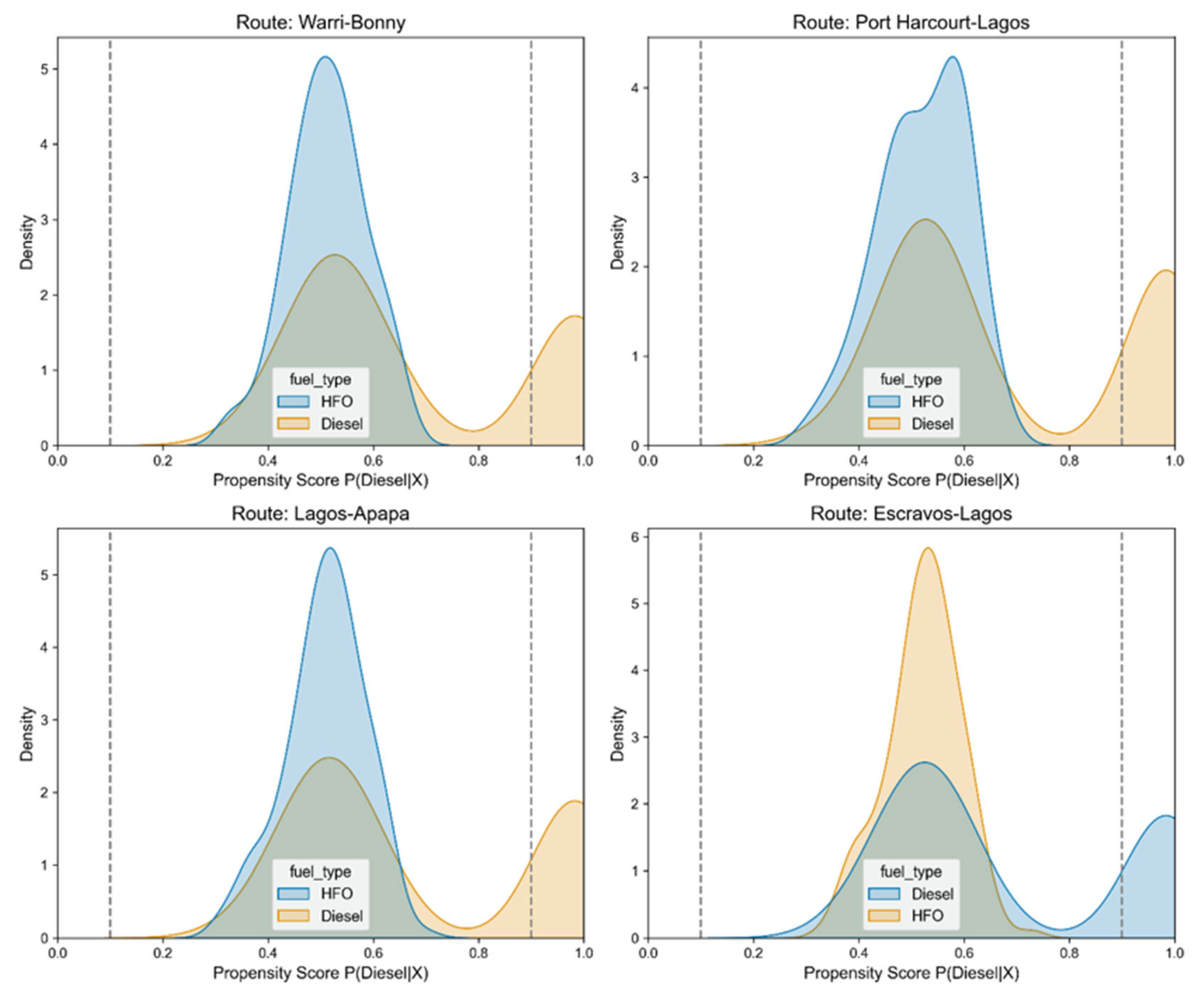
Treatment assignment reflects operational fuel policies rather than randomized switching. Many vessel–route pairs are effectively mono-fuel; however, some vessels operate multiple corridors and appear with different fuels across routes. Accordingly, causal effects are interpreted as voyage-level contrasts between Diesel and HFO under comparable route, season, and weather conditions rather than as within-vessel before–after switches on the same leg. Identification relies on overlap (common support) in the covariate space (distance, season, weather category, ship attributes, and engineered route-relative metrics). Propensity-score diagnostics are visualized in Figure 4.

ATE via Double/Debiased Machine Learning (DML). We estimated the ATE using Double/Debiased Machine Learning with cross-fitting [41]. Flexible nuisance models were fitted for the outcome m(X) ≈ E[Y|X] and the propensity score e(X) ≈ P(T = 1|X). Cross-fitting yields orthogonalized residuals that reduce regularization bias when estimating the treatment effect.

CATE via Causal Forests. To capture heterogeneity in fuel-switching benefits, we estimated CATEs using Causal Forests with 1000 trees, following [42]. For a covariate profile X = x, the CATE is:

$$\tau \left(x\right)=E\left[Y\left(1\right)-Y\left(0\right)|X=x\right],$$

(4)

For interpretability and to avoid data dredging, we summarized heterogeneous effects primarily at the route × season level, focusing on cells with adequate overlap between fuels.

Covariate set and overlap diagnostics. The covariate set X includes core operational variables (distance_nm, season_bin, weather_category), ship-level descriptors (ship_type), and engineered route-relative metrics (route_difficulty_score, intensity_gap). Propensity scores are estimated via logistic regression:

$$e\left(X\right)=P\left(T=1|X\right)$$

(5)

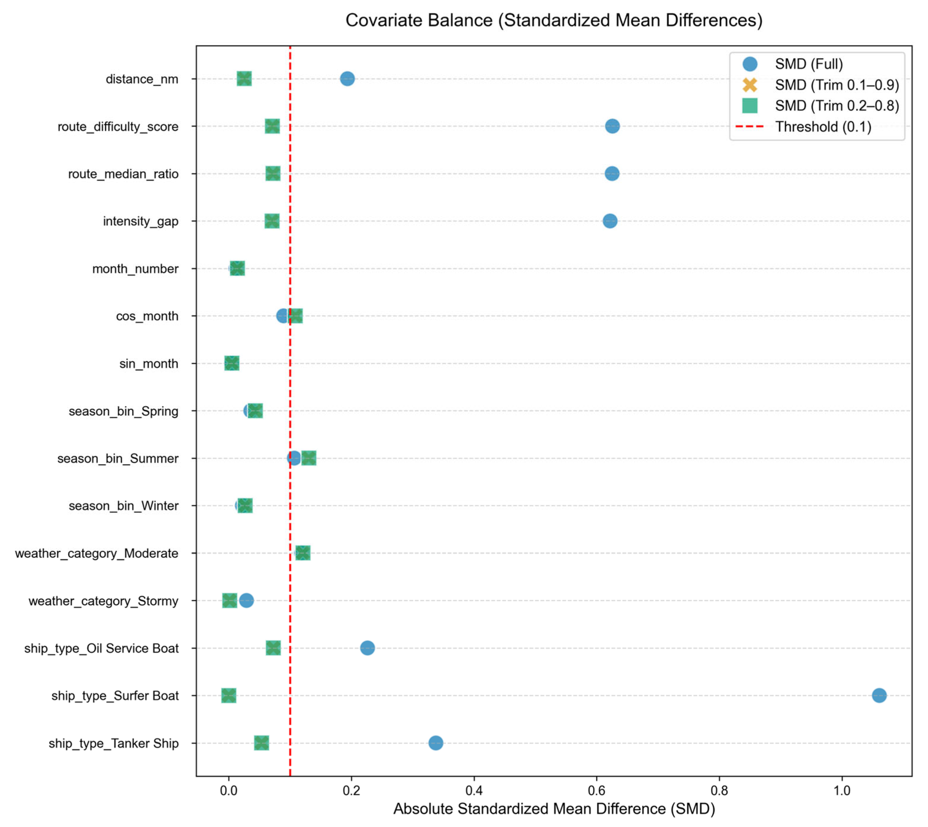
and Figure 4 suggests non-zero overlap within the observed covariate space; to assess robustness, we additionally report the ATE/CATE estimates on trimmed samples restricting $e\left(X\right)$ to [0.10, 0.90] and [0.20, 0.80] and we provide complementary overlap/balance diagnostics in Appendix C.

2.7.1. Identification Strategy and Operational Pathways

Fuel choice in coastal shuttle operations is an operational decision and is therefore structurally endogenous to voyage planning. In practice, operators may select Diesel versus HFO based on bunkering availability and contracting, port/terminal constraints, safety-driven maneuvering requirements in constrained approaches, cost planning, and maintenance practices. In our dataset, these operational pathways are proxied by the observed covariate set X capturing route geometry and stress (distance_nm, route_difficulty_score, route_median_ratio, intensity_gap), environmental conditions (weather_category), seasonal operating regimes (season_bin and the seasonal encodings used in the feature set), and vessel class (ship_type). Under the potential-outcomes framework, we interpreted the estimated ATE/CATE as conditional causal contrasts only under three standard assumptions: (i) consistency/SUTVA (each voyage’s outcome corresponds to its observed fuel_type and is not affected by other voyages), (ii) conditional ignorability of fuel choice given X (unconfoundedness), and (iii) positivity (overlap) within the observed covariate space. While unconfoundedness cannot be proven in observational data, the identification argument here is that conditioning on these operational proxies removes the dominant drivers that jointly affect fuel choice and CI_kg_per_nm. Building on the DML formulation above, Double/Debiased Machine Learning targets selection bias by separately learning the treatment-assignment mechanism $e\left(X\right) = P(T = 1|X)$ and the outcome mechanism $m\left(X\right) = E\left[Y\right|X]$, and then orthogonalizing the residual variation via cross-fitting to reduce bias from flexible nuisance models [41]. To satisfy the strict overlap assumption and mitigate endogeneity, we inspected the propensity score distributions and applied trimming to exclude voyages with extreme treatment probabilities (outside the [0.05, 0.95] range), ensuring that comparisons between HFO and Diesel were made only within a valid common support region. The propensity model in Equation (5) provides an empirical summary of the assignment mechanism and helps detect near-deterministic fuel policies for specific operational profiles. Positivity was assessed empirically through overlap in estimated propensity scores between treated (Diesel) and control (HFO) voyages; Figure 4 suggests non-zero overlap within the observed common-support region (e.g., comparable profiles such as a stormy 100 nm voyage). However, because fuel policies may still be partially structured at corridor and vessel levels, all causal contrasts were interpreted within the observed support (and conditional on X), and we avoided extrapolation to domains where one fuel is rarely or never observed. Appendix C reports additional overlap, balance, trimming, and sensitivity diagnostics that make the supported domain of the causal contrasts explicit.

2.7.2. Sensitivity to Unobserved Confounding

Even after conditioning on X, unobserved factors such as load condition, hull/propeller fouling, draft/trim, and congestion or currents may induce residual confounding in observational voyage data. We therefore complemented the main estimates with a partial-R²-based omitted-variable sensitivity framing that characterizes how strong an unmeasured confounder would need to be (in incremental explanatory power for both the treatment and outcome models) to materially change the ATE conclusions; the calculations are summarized in

Table A8. Sensitivity summary for unobserved confounding.

Sensitivity Quantity	Value	Interpretation
Robustness Value (RVq = 1RVq = 1)	1.65%	Unobserved confounders would need to explain 1.65% of the residual variance to explain away the estimated effect.
ATE without Distance	0.0000	No change. Distance is well-balanced.
ATE without Weather	0.0000	No change. Weather impact is handled.
ATE without Route Metrics	0.0024	Slight shift, confirming route metrics capture important confounding.

. In addition, we performed a leave-one-covariate-block-out robustness check, re-estimating ATE/CATE after removing (i) distance-related terms, (ii) weather/season terms, (iii) ship_type, and (iv) engineered route-stress proxies (route_difficulty_score, route_median_ratio, intensity_gap). Any instability across these perturbations was reported and interpreted as evidence of fragility, whereas stability supports the interpretation of the estimates as conditional contrasts within the observed support. Quantitative results for these checks are reported in Appendix C.

2.8. Summary of Outputs and Reproducibility Notes

The unified pipeline yields five decision-relevant outputs: (i) point forecasts of voyage-level emission intensity on unseen corridors (LightGBM under LORO), (ii) distribution-free prediction intervals with finite-sample coverage guarantees (split-conformal), (iii) inputs for risk-oriented screening based on the uncertainty envelope (e.g., exceedance-type indicators derived from conformal bounds), (iv) causal estimates of fuel switching effects at both the global (ATE) and heterogeneous (CATE) levels (DML and Causal Forests), and (v) an economic integration layer based on cost intensity concepts under alternative carbon-pricing scenarios. Appendix A documents the source dataset structure and limitations, while Appendix B details the construction of the derived voyage-level panel and provides the full variable dictionary, enabling transparent replication of feature construction and modeling inputs.

3. Results

Results at a glance:

• Under strict Leave-One-Route-Out evaluation, unseen-route emission-intensity forecasting achieved a MAE ≈ 40.7 kg CO₂/nm (

  Table 3. Route-level predictive performance on unseen test sets (Leave-One-Route-Out Cross-Validation).

  Fold	Unseen Route (Test Set)	MAE (kg/nm)	RMSE (kg/nm)	R2
  1	Port Harcourt–Lagos	33.73	41.31	–1.14
  2	Lagos–Apapa	45.00	52.58	–2.51
  3	Escravos–Lagos	46.95	54.72	–2.70
  4	Warri–Bonny	37.03	44.07	–1.72
  Avg.	Global Average	40.68	48.17	–2.02

  ), while R² can be negative due to corridor-level level shifts.
• The 90% split-conformal prediction intervals achieved 100% empirical coverage on held-out routes, supporting uncertainty-aware compliance planning (Section 3.1).
• SHapley Additive exPlanations (SHAP) analysis indicates the model relies on route-relative difficulty metrics and a physics-consistent distance effect, supporting robust generalization beyond route identifiers (Section 3.2).
• In the causal layer, DML estimated a near-zero global average Diesel-vs.-HFO effect (ATE = −0.072 kg CO₂/nm, 95% CI [−0.155, 0.011]), while Causal Forests revealed strong route–season heterogeneity (CATEs from −74 g to +29 g CO₂/nm) (Section 3.3).
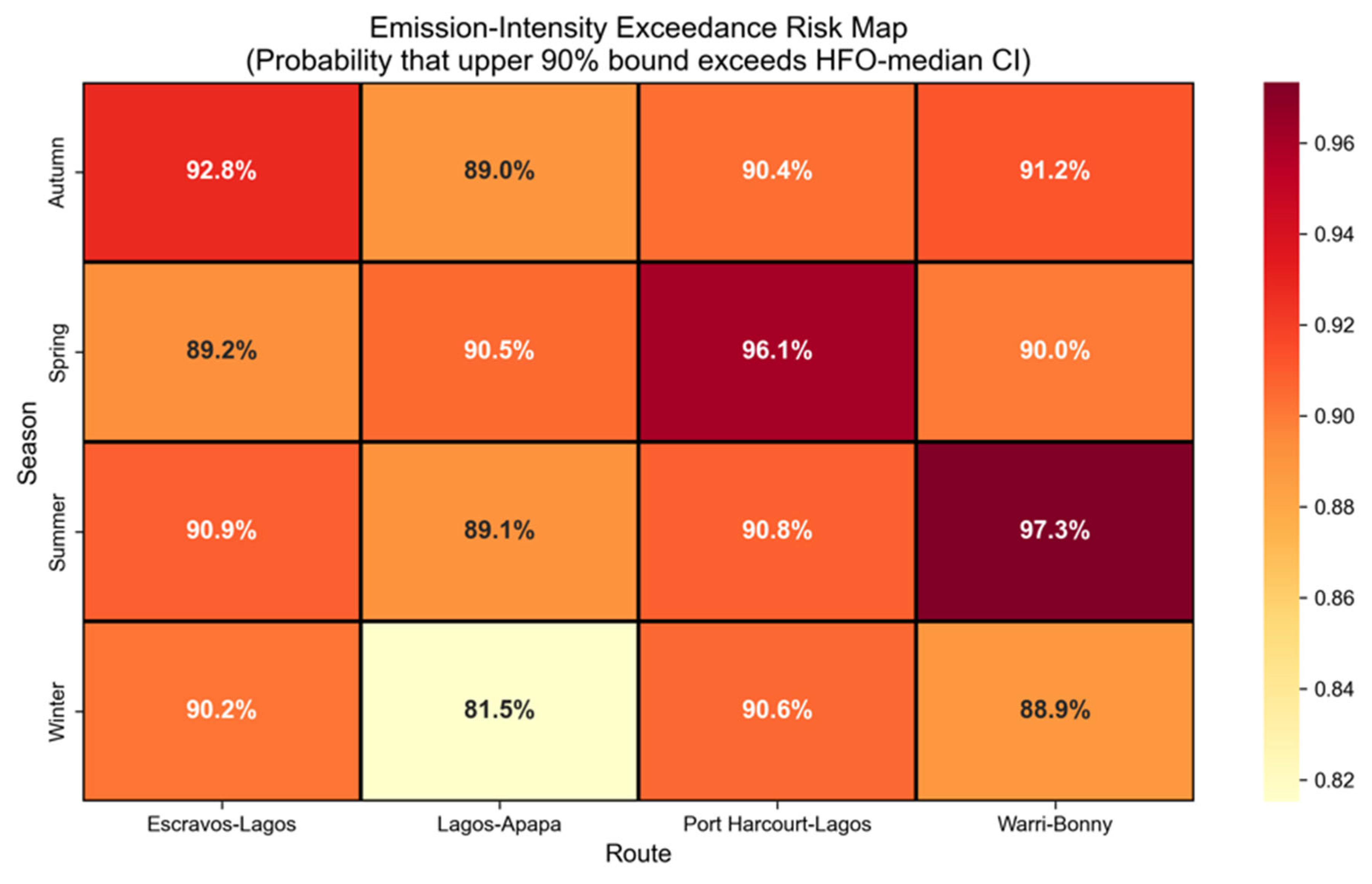
• A conformal-interval–based Exceedance Risk Map indicates persistently high probabilities (≈81.5–97.3% across route–season cells) that the upper 90% prediction bound exceeds historical HFO median intensity, prioritizing corridors for SEEMP Part III interventions (Section 3.4).
• In the economic integration, Total Cost Intensity (TCI) results indicate that selective Diesel use on demanding corridors becomes economically attractive when carbon prices approach ~100 USD/tCO₂, with further convergence at higher carbon prices (Section 3.5).

This section reports the empirical performance of the proposed causal–conformal framework. We first evaluate the predictive accuracy of the monotonic LightGBM model and its distribution-free uncertainty quantification under a strict leave-one-route-out (LORO) scheme. We then examine how fuel switching from HFO to Diesel affects emission intensity, both on average and across heterogeneous route–season cells. Finally, we translate these environmental results into compliance risk and cost outcomes through an Emission-Intensity Exceedance Risk Map and a Total Cost Intensity (TCI) analysis under alternative carbon pricing scenarios.

3.1. Unseen-Route Forecasting and Uncertainty Quantification

The monotonic LightGBM model exhibited robust generalization when deployed on completely unseen coastal corridors. Across the four leave-one-route-out (LORO) folds, the model attained a global mean absolute error $\left(MAE\right) \mathrm{of} 40.7 \mathrm{kg} {\mathrm{CO}}_2/\mathrm{nm}$ on the held-out routes. Route-level performance metrics are summarized in Table 3.

The highest errors occurred on Escravos–Lagos $(MAE \approx 46.95 \mathrm{kg} {\mathrm{CO}}_2/\mathrm{nm}, RMSE \approx 54.72 \mathrm{kg} {\mathrm{CO}}_2/\mathrm{nm})$ and Lagos–Apapa $(MAE \approx 45.00 \mathrm{kg} {\mathrm{CO}}_2/\mathrm{nm}, RMSE \approx 52.58 \mathrm{kg} {\mathrm{CO}}_2/\mathrm{nm}),$ reflecting the high operational variability of short, congested river passages and intra-port shuttles where steady cruising is rare. In contrast, the longer Port Harcourt–Lagos route displayed the lowest error $(MAE \approx 33.73 \mathrm{kg} {\mathrm{CO}}_2/\mathrm{nm}, RMSE \approx 41.31 \mathrm{kg} {\mathrm{CO}}_2/\mathrm{nm}),$ consistent with a larger share of stable steaming in open-coast conditions. Averaging over folds yielded a global $MAE \mathrm{of} 40.68 \mathrm{kg} {\mathrm{CO}}_2/\mathrm{nm},$ which is numerically consistent with the rounded value of 40.7 kg CO₂/nm reported at the fleet level.

The negative R² values observed across all folds do not indicate that the model is uninformative; rather, they reflect the severity of the distribution shift inherent to the unseen-route setting. In the LORO protocol, each test fold corresponds to a route whose mean emission intensity can differ substantially from the training-set average. Using the training-route mean as a baseline therefore induces a strong level shift, against which even well-calibrated predictions can yield negative R² when evaluated in the usual way. In this context, MAE and RMSE remain the more interpretable measures of performance, while negative R² primarily signals that unseen routes possess different absolute intensity baselines rather than that the model fails to learn meaningful structure. Indeed, the route-level results in Table 3 show that operational difficulty is still ranked in a manner consistent with the underlying geometry and stress profile of each corridor, motivating the distribution-free adjustment provided by the split-conformal framework.

For uncertainty quantification, the LightGBM predictor was wrapped in a 90% split-conformal scheme calibrated under the same LORO protocol. Across all test folds, the split-conformal prediction intervals achieved 100% empirical coverage, with a calibrated interval half-width $\hat{q} = 81.2 \mathrm{kg} {\mathrm{CO}}_2/\mathrm{nm}$. These bands are intentionally conservative: the pooled calibration residuals are strongly influenced by difficult segments such as Lagos–Apapa and Escravos–Lagos, where short distances, frequent maneuvering and shallow-water effects generate heavy-tailed errors. The resulting prediction intervals therefore expand to accommodate worst-case covariate shifts on completely unseen corridors. From a regulatory perspective, this conservatism is desirable, as it reduces the risk of underestimating emissions and ensures that regulatory compliance risks are not an understated critical requirement in safety-critical maritime reporting where false negatives carry significant penalties. These intervals underpin the Emission Intensity Exceedance Risk Map discussed in Section 3.4.

Key takeaway: Under strict unseen-route deployment, point-prediction metrics are constrained by corridor-level distribution shifts, whereas conformal intervals provide deployment-relevant uncertainty bounds for compliance-oriented planning.

3.2. Model Interpretability and Physics-Informed Validation

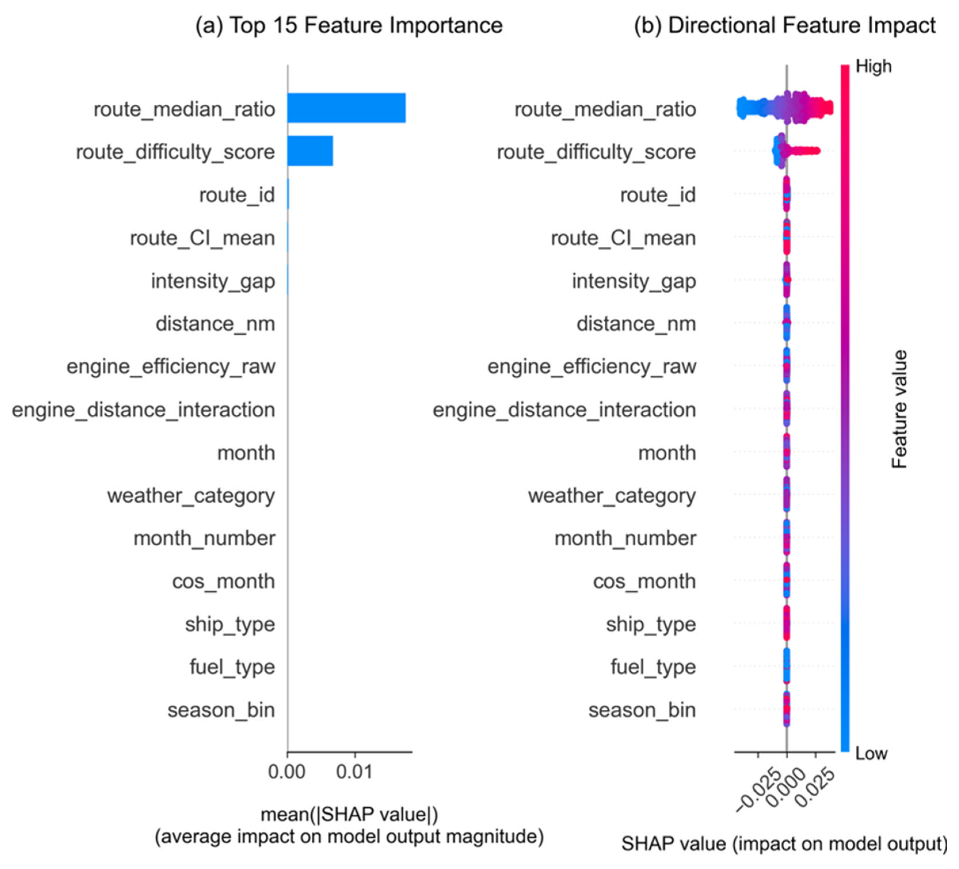
To ensure that the predictive model captured transferable operational physics rather than route-specific artifacts, we analyzed its behavior using SHAP (SHapley Additive Explanations). The global feature-importance plot in Figure 5 shows that route-relative metrics, in particular route_median_ratio and route_difficulty_score (and, to a lesser extent, intensity_gap), dominated the prediction of emission intensity on unseen routes. This dominance indicates that the model relies on deviations from appropriate baselines—how “difficult” a voyage is relative to typical voyages—rather than memorizing absolute route identifiers, which is a key requirement for robust unseen-route generalization.

The SHAP summary plot in Figure 5 provides a direct validation of the physics-informed monotonicity constraint imposed on voyage distance. High values of distance_nm (red points) are consistently associated with negative SHAP values, meaning that longer voyages systematically push the predicted CI downward on a per-nautical-mile basis. This pattern is precisely what the hydrodynamics of coastal operations suggest: longer passages allocate a larger share of time to efficient cruising and a smaller share to fuel-intensive maneuvering and hoteling. The fact that SHAP aligns with the imposed non-increasing constraint on distance, even for routes that were never seen in training, reinforces confidence that the model has internalized a physically meaningful distance–intensity relationship rather than exploiting spurious correlations.

Taken together, the SHAP analysis and the monotonicity constraint show that the LightGBM model respects basic maritime physics while leveraging route-relative features to accommodate heterogeneity in geometry, weather, and congestion across the Nigerian coastal network.

Key takeaway: SHAP patterns confirm that the model relies on route-relative stress features and a physically consistent distance–intensity relationship, supporting transferability beyond route memorization.

3.3. Average Versus Heterogeneous Effects of Fuel Switching

These causal contrasts were interpreted within the observed overlap/common-support region of this single-operator dataset; $route\times season$ cells with limited support were not over-interpreted. Complementary overlap, balance, trimming, and sensitivity diagnostics that clarify the supported domain are reported in Appendix C.

The effect of switching from HFO to Diesel on voyage-level emission intensity was next examined after adjusting for operational confounding. Using Double/Debiased Machine Learning, the Average Treatment Effect (ATE, arithmetic mean) of Diesel relative to HFO was estimated as −0.072 kg CO₂/nm, with a 95% confidence interval of [−0.155, 0.011]. Because this interval includes zero (p > 0.05), the global average effect is statistically indistinguishable from zero. In other words, when averaged across all voyages in the dataset, no guarantee is provided that a blanket, fleet-wide switch from HFO to Diesel would lead to a systematic reduction in emission intensity.

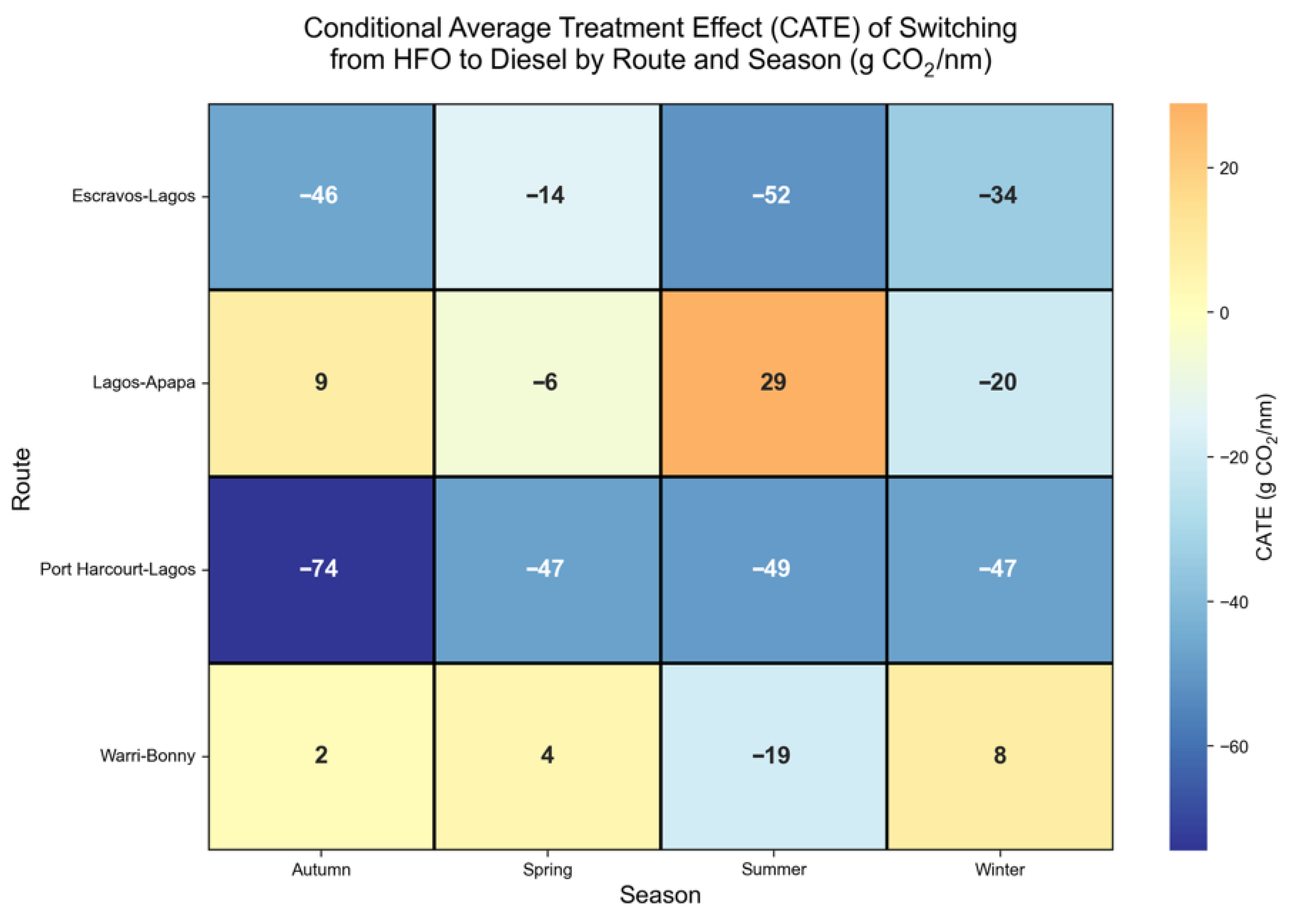
This absence of a strong global effect does not imply that fuel switching is irrelevant; rather, it indicates that positive and negative effects coexist and largely cancel out in aggregate. The Causal Forest analysis revealed substantial treatment-effect heterogeneity across route–season cells. The CATE map in Figure 6 shows that emission reductions concentrated in specific high-stress operational regimes, while other segments exhibited neutral or even adverse outcomes. The CATE map in Figure 6 illustrates these contrasts: on the Port Harcourt–Lagos route during Autumn, switching from HFO to Diesel reduced emission intensity by 74 g CO₂/nm, corresponding to a substantial improvement in CI on a long, hydrometeorologically demanding passage. In contrast, on the short Lagos–Apapa route during Summer, Diesel increased emissions by 29 g CO₂/nm, reflecting the inefficiencies of Diesel engines under low-load, maneuvering-dominated conditions.

These heterogeneous patterns are consistent with the underlying route geometry and operating environment. On Port Harcourt–Lagos, particularly in Autumn, vessels encounter long stretches of steady steaming interspersed with current-affected bar crossings. Such conditions push the main engine closer to its optimal loading regime and allow Diesel’s thermodynamic advantages over HFO to translate into the observed emission savings of up to 74 g CO₂/nm. In contrast, the Lagos–Apapa leg is a very short intra-port shuttle; it is dominated by low-speed maneuvering, short acceleration–deceleration cycles, and extended periods at or near idle power. Under these part-load and stop–start conditions, Diesel engines operate far below their design efficiency bands and may exhibit higher specific fuel consumption than HFO, explaining the positive CATE values (emission penalties) observed on this segment.

Overall, the joint ATE–CATE results suggest that uniform fuel switching policies are inefficient. Instead, Diesel should be deployed selectively on high-stress routes and seasons where it provides clearly beneficial emission reductions, while HFO can remain preferable on low-stress, maneuvering-dominated legs where Diesel offers little or no environmental advantage.

Key takeaway: The decision-relevant signal is heterogeneity: despite a near-zero global ATE, route–season CATEs indicate where Diesel is beneficial versus counterproductive under comparable operating conditions.

3.4. Compliance Risk and Economic Implications: Exceedance Risk

To connect predictive uncertainty with regulatory compliance, we constructed an Emission-Intensity Exceedance Risk Map based on the split-conformal intervals. For each route–season cell, the map reports the probability that the upper bound of the 90% conformal prediction interval exceeds the historical HFO median emission intensity on that corridor.

As shown in Figure 7, the resulting probabilities were high across the operational domain, ranging from 81.5% on Lagos–Apapa in winter to 97.3% on Warri–Bonny in Summer. This apparent saturation is a direct consequence of the conservative, distribution-free calibration: to guarantee coverage on completely unseen routes, the conformal procedure constructs intervals wide enough to encompass the worst-case residuals observed in the most challenging operating regimes.

From a risk-management perspective, high exceedance probabilities should therefore be interpreted as a feature rather than a flaw. They indicate that given current operational practices, even the upper-bound scenarios for many route–season combinations are likely to surpass historical HFO medians and thus warrant close monitoring in a CII-oriented compliance framework. Crucially, the Exceedance Risk metric integrates both the central tendency and the uncertainty of predicted CI, providing a more robust signal than point forecasts alone.

In practical terms, the Exceedance Risk Map can be embedded into Ship Energy Efficiency Management Plan (SEEMP) Part III processes as a route–season screening tool. Cells with persistently high exceedance probabilities flag segments where proactive intervention is most needed. Fleet managers can use these signals to prioritize speed optimization, weather routing, trim and engine-tuning checks, or targeted fuel switching prior to dispatch, thereby integrating statistically rigorous risk information into routine voyage planning and compliance reporting. In the next subsection, we complement this risk-based view with an explicit cost analysis through the Total Cost Intensity metric under alternative carbon pricing regimes.

Key takeaway: Carbon pricing and uncertainty together shape actionability—TCI identifies when selective switching becomes economically plausible, while exceedance risk prioritizes where compliance margins are most likely to be strained.

3.5. Total Cost Intensity

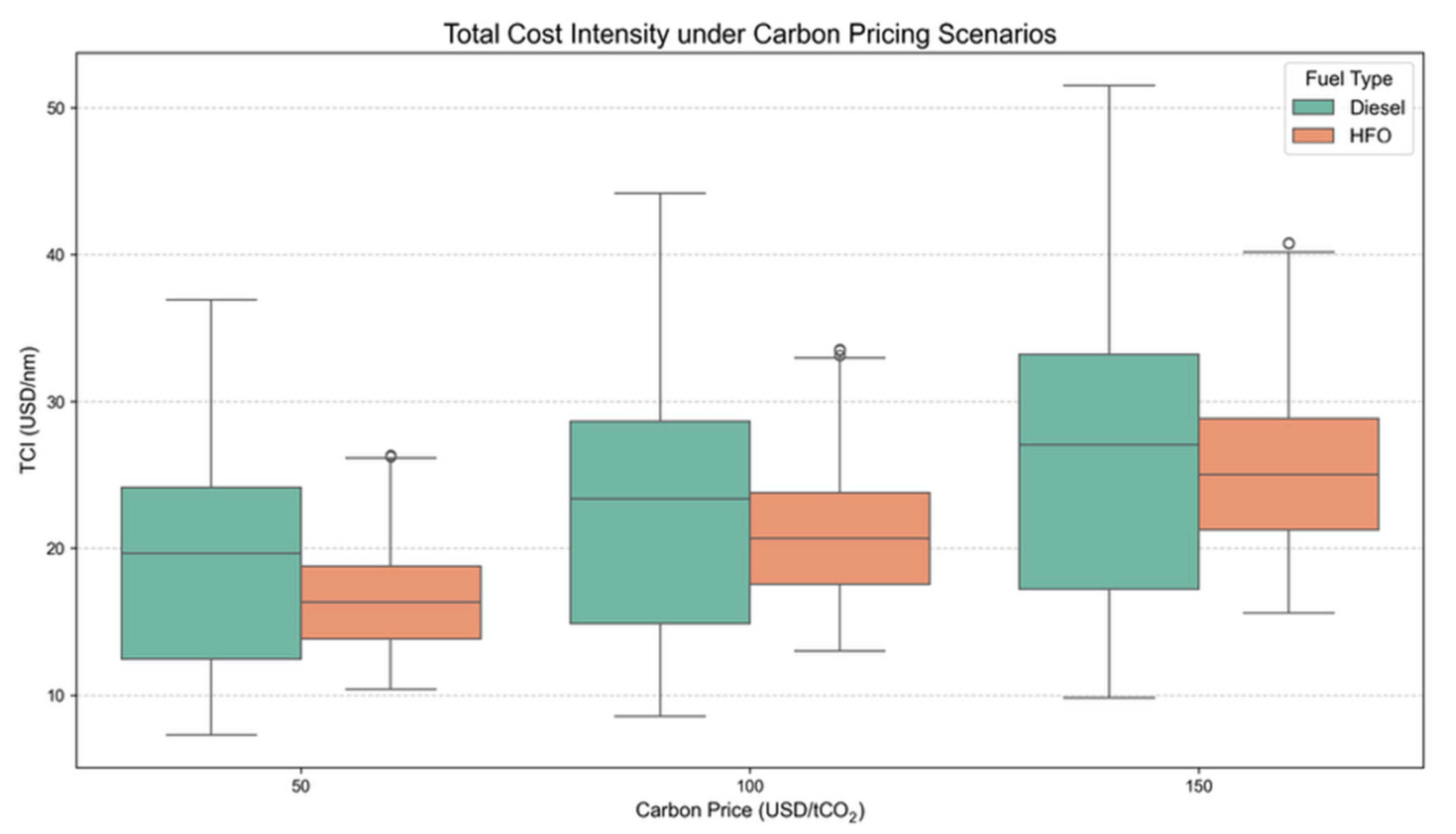
To integrate environmental outcomes with economic considerations, we analyzed Total Cost Intensity (TCI) in USD per nautical mile under three carbon pricing scenarios: 50, 100, and 150 USD/tCO₂. Figure 8 displays the TCI distributions for HFO and Diesel voyages. Under the 50 USD/tCO₂ scenario, HFO retained a clear cost advantage: its lower bunker price dominated the modest emission-based surcharge, and the TCI distributions of the two fuels remained well separated. As the carbon price increased to 100 and then 150 USD/tCO₂, however, the TCI gap narrowed substantially. At 150 USD/tCO₂, the Diesel and HFO distributions exhibited significant overlap, indicating that Diesel becomes economically viable for a non-trivial subset of voyages—particularly those high-stress routes identified in Section 3.3 where Diesel also delivers the largest physical emission reductions.

To illustrate the economic magnitude of these differences, consider a typical 150 nm coastal voyage. A TCI gap of 4–6 USD/nm between fuels translates into an additional 600–900 USD per trip, which is material for short-sea operators facing thin margins and frequent sailings. The threshold of approximately 100 USD/tCO₂ at which Diesel becomes cost-competitive on the most challenging routes is broadly consistent with projected carbon price ranges under emerging EU ETS and FuelEU Maritime regimes. This alignment suggests that the crossover points observed in our TCI analysis are not mere theoretical artifacts but fall within plausible near-term regulatory scenarios. In combination with the heterogeneous CATE estimates, the TCI results support a strategy of selective Diesel deployment on high-stress routes where both environmental and economic incentives are aligned.

4. Discussion

The results were intentionally generated under a deployment-like design: forecasting and uncertainty quantification were evaluated under a strict leave-one-route-out protocol, while fuel-switching effects were interpreted as conditional contrasts rather than randomized outcomes. The aim of this discussion is therefore not to “celebrate” a single predictive metric, but to clarify what the combined predictive–uncertainty–causal outputs mean for corridor-level decision-making under compliance pressure and carbon-cost exposure. We synthesize three messages. First, when deployment involves domain shift, uncertainty-aware bounds can be more decision-relevant than point accuracy on unseen routes. Second, heterogeneity (CATE) should be treated as an operational decision map rather than a statistical curiosity, and it can overturn blanket “average-effect” rules. Third, these corridor-level tools matter because the sector’s decarbonization trajectory is increasingly shaped by a policy stack that rewards auditable, risk-aware operational planning. We close by translating findings into actionable ship-side and port-side implications, and by clarifying scope conditions under which the claims should (and should not) be generalized.

4.1. Uncertainty Guarantees and Physics-Informed Robustness

The results demonstrate that accurate voyage-level emission-intensity forecasting is achievable even under a stringent leave-one-route-out protocol. The physics-informed monotonic LightGBM model attained a global mean absolute error of 40.7 kg CO₂/nm on completely unseen corridors.

The observation of negative $R²$ values and an MAE of ~40.7 kg CO₂/nm warrants critical context. In a Leave-One-Route-Out (LORO) setting, the model faces a complete distribution shift; the ‘unseen’ route often operates at a fundamentally different intensity baseline than the training routes due to static geometric factors (e.g., river depth vs. open sea). A naïve baseline model predicting the global training mean for all test voyages would yield comparable absolute errors but would fail to capture intra-voyage dynamics. The practical utility of the proposed framework, therefore, does not rely on achieving a high $R²$ on unseen routes—which is mathematically impossible without target data—but on two other capabilities: (i) Risk Management, where conformal prediction intervals successfully adapt to this uncertainty providing a statistically guaranteed upper bound; and (ii) Causal Sensitivity, where the ML model, unlike a static baseline, learns valid physical derivatives allowing it to correctly estimate the marginal effect of fuel switching.

Consequently, the 90% split-conformal prediction intervals achieved 100% empirical coverage on the held-out routes. While coverage exceeding the nominal level might initially appear overly conservative, it is an expected and desirable outcome when calibration is performed under covariate shift and the method is required to remain valid on unseen corridors. By aggregating residuals across all folds, including the most challenging legs such as Lagos–Apapa and Escravos–Lagos, the calibration procedure inflates the conformal half-width to a global value of 81.2 kg CO₂/nm that reflects worst-case conditions. In cells where hydrometeorology, congestion, or river-mouth constraints induce strong variability, wider intervals act as a statistical safety buffer, reducing the risk of under-reporting emissions or misclassifying voyages near compliance thresholds.

We specifically examined the validity of the monotonic distance constraint on short, congested segments like the Lagos–Apapa corridor. Although maneuvering adds noise, our diagnostics on the raw data confirm that the correlation between distance and emission intensity remains strongly positive; thus, the monotonic constraint serves as an effective regularizer that prevents the model from overfitting to transient congestion anomalies.

Two design choices reinforce that these outputs are deployment-oriented rather than retrospective curve-fitting: (i) the strict leave-one-route-out protocol, and (ii) leakage-aware out-of-fold constructs, which force the model to operate under genuine domain shift. The SHAP analysis further reinforces this robustness. Relative features—such as route-median deviations and route-level difficulty scores—consistently dominated the global SHAP-importance rankings, indicating that meaningful, route-relative operational physics are captured rather than mere memorization of raw route identifiers. At the same time, the monotonicity constraint imposed on distance_nm is clearly reflected in the SHAP sign pattern: longer voyages systematically exhibited negative SHAP contributions, confirming that the model has internalized the hydrodynamic principle whereby an increased share of steady cruising reduces emission intensity on a per-nautical-mile basis.

Key implication: Even when unseen-route point forecasts exhibit level shifts, uncertainty-aware upper bounds remain practically actionable for compliance-oriented screening and planning.

4.2. What “Heterogeneity” Means Operationally (ATE vs. CATE)

Average treatment effects (ATE, arithmetic mean) provide a compact summary, but operational decisions are made on specific corridor–season profiles where marginal impacts can vary. In this setting, heterogeneous effects (CATE) are best read as a decision map: they indicate where switching from HFO to Diesel is expected to reduce emission intensity and where it may be neutral or even adverse, conditional on the observed operational context. This is why heterogeneity should be treated as a feature, not a nuisance—especially in coastal operations where route geometry, maneuvering intensity, and weather regimes jointly shape both fuel selection and emissions response. A single global “fuel switching rule” can therefore be misleading, even when the average effect appears benign.

A physically interpretable way to read the heterogeneity is to link fuel effects to operating regimes. On longer, higher-stress passages with a larger share of steady open-coast steaming, main engines are more likely to operate nearer their efficient loading band, so changes in fuel properties can translate into measurable shifts in intensity per nautical mile. In contrast, on short, maneuvering-dominated legs—where acceleration–deceleration cycles, low-speed segments, and idling near terminal approaches are more prominent—engines spend more time in part-load regimes, and the expected direction of a fuel switch can attenuate or even reverse. In other words, the “same” fuel switch can behave differently depending on whether the voyage is dominated by steady cruising or by stop–start maneuvering and constrained approaches.

Accordingly, the interpretative value of the causal layer is prioritization, not universal prescriptions. The operationally appropriate use is to target switching (and complementary levers) to the corridor–season cells where conditional contrasts are favorable and counterfactual support is credible, while recognizing that other cells may be better served by speed management, maintenance planning, or port-side measures.

Key implication: The CATE layer is most useful as a targeted screening tool that supports selective interventions rather than uniform fleet-wide fuel-switching mandates.

4.3. International Context and Sector Evidence

Coastal shipping decarbonization is increasingly shaped by a portfolio of policy and market pressures that reward measurable efficiency and penalize carbon-intensive operations, including intensity-based schemes, emerging carbon-pricing mechanisms, and procurement expectations from cargo owners. Across international assessments of the energy transition, a recurring theme is that hard-to-abate transport segments require layered strategies: near-term operational efficiency gains, medium-term fuel and engine transitions constrained by bunkering and port readiness, and robust monitoring and verification that remains credible under real-world variability. In that sense, sector narratives (often grounded in global energy-transition evidence) consistently emphasize decision robustness and implementation feasibility over any single “best” model metric.

Within that broader framing, the contribution of this study is not a new sector-wide statistic but a corridor-level decision lens that makes variability, domain shift, and heterogeneity explicit. The leave-one-route-out results highlight that deployment often entails distribution shift, where absolute baselines can differ materially across corridors; this motivates conservative uncertainty quantification rather than over-reliance on point forecasts. In parallel, the cost-intensity framing shows how carbon pricing can change the attractiveness of operational choices, enabling the same emissions insights to be interpreted as cost exposure under plausible policy trajectories (including scenarios where carbon prices approach levels that narrow the cost gap between fuels on the most challenging routes). Together, these elements align with the structure of international sector discussions: “measure” (credible monitoring under variability), “manage” (risk-aware decision thresholds), and “mitigate” (targeted levers where the marginal benefit is plausibly positive).

Key implication: Corridor-level uncertainty bounds, heterogeneity maps, and cost-intensity stress tests translate broad policy and sector pressures into operationally interpretable route–season prioritization.

4.4. Policy and Sustainability Implications (Ship-Side + Port-Side)

From a policy and operations perspective, the key step is to treat uncertainty and heterogeneity as first-class planning inputs rather than residual noise. The exceedance-risk outputs based on conformal upper bounds can be used to flag corridor-season cells where the probability of breaching an intensity benchmark is high, while the carbon-pricing analysis frames how the same physical variability propagates into cost exposure. Fuel-switching guidance should then be applied selectively—only within the operational profiles where the conditional contrast is favorable and where comparable counterfactual voyages exist—while other cells may be better served by operational levers or port-side mitigation.

4.4.1. Economic Sensitivity and Market Drivers

The economic viability of fuel switching is fundamentally driven by the spread between HFO and Marine Diesel prices relative to the imposed carbon price. Our finding that Diesel becomes cost-competitive only at ~100 USD/tCO₂ is therefore conditional on the baseline market conditions assumed in this study, rather than a universal threshold. Beyond carbon pricing itself, vessel- and regime-specific operating conditions (engine load, maneuvering share, and auxiliary/hoteling demand) shape the Total Cost Intensity (TCI) by affecting effective specific fuel consumption and the extent to which carbon-cost components accumulate under different route–season operating profiles.

Table 4. Summary of Economic Variables and Sensitivity Drivers (descriptive transparency table; no additional sensitivity computations are introduced).

Variable	Baseline Value	Range/Scenario (Qualitative)	Operational Impact	Sensitivity/Effect on Crossover Point
HFO Price	400 USD/ton	Market-dependent; cheaper HFO higher crossover	High	A decrease in HFO price widens the cost gap, pushing the required carbon tax above ~100 USD/tCO2.
Diesel Price	700 USD/ton	Market-dependent; narrower spread lower crossover	High	The bunker price spread (≈300 USD/ton in our data) is the primary barrier; if the spread narrows, the crossover carbon price drops proportionally.
Carbon Price	0–150 USD/tCO2	Policy lever (0–150 in scenarios)	High	At carbon prices around and above ~100 USD/tCO2, the carbon-cost component begins to outweigh the bunker price spread.
Specific Fuel Consumption (SFOC)	Variable (engine load dependent)	Load-dependent; port/maneuvering increases breakeven	Moderate	Diesel engines lose efficiency at low loads (port/maneuvering), increasing the breakeven carbon price on short routes such as Lagos–Apapa.
Auxiliary Load	~10–15% of total	~10–15%; higher hoteling favors HFO	Low–Moderate	Assumed constant proportional to hoteling time; higher auxiliary loads generally favor HFO due to lower base cost.
CO2 emission factor (HFO vs. Diesel)	Fuel-specific (standard factors used in cost construction)	Fuel-specific; secondary	Low–Moderate	Secondary driver; the bunker price spread dominates the crossover point under the assumed market conditions.
Operational regime (route × season: weather, maneuvering share, hoteling time)	Captured via season_bin, weather_category, and route/distance proxies	Seasonal/route-specific; shifts breakeven	Moderate	Short/maneuvering-heavy legs raise the effective breakeven; long steady-steaming legs lower it.

summarizes the key economic variables used in this study, their baseline values, qualitative “range/scenario” descriptors (without additional computations), and the direction by which each factor is expected to shift the breakeven (crossover) carbon price.

As shown, the ~100 USD/tCO₂ crossover should be interpreted as conditional on the baseline bunker price spread (≈300 USD/ton) observed during the study period, not as a universal constant. If global oil market dynamics were to compress this spread—for instance, due to higher refinery supply of distillates or regulatory shifts that make HFO structurally more expensive—the carbon price required to incentivize switching would decrease. Conversely, in a market with relatively cheap HFO and a widespread, even aggressive carbon pricing may struggle to bridge the gap without complementary operational or institutional incentives (e.g., differentiated port dues or corridor-level programs).

Seasonality and route regime matter because they alter the operating envelope in which costs are realized (e.g., maneuvering share, congestion exposure, and hoteling time), thereby shifting the effective breakeven in a corridor–season–specific way. Thus, the crossover should be interpreted at the corridor–season level, not as a single global constant.

4.4.2. Port-Side Enablers and Near-Coastal Mitigation

Complementary port-side measures can amplify the benefits of ship-side interventions, particularly for short sea routes with frequent turnaround. Energy management systems can reduce idle and auxiliary loads, while shore power and near-terminal electrification can decouple berth emissions from onboard generation. In parallel, integrating renewables into port microgrids can lower the effective carbon intensity of electrified operations, thereby improving the total system-level benefit of fuel switching and speed management. These port-side levers are particularly relevant in corridors where operational constraints limit the feasibility of aggressive ship-side retrofits.

A practical “how to use” synthesis for operators and regulators is as follows:

• Use exceedance-risk outputs (based on the conformal upper bound) as a route–season screening layer for voyage planning and internal compliance checks, focusing attention on corridor–season cells where compliance margins are most fragile.
• Apply selective fuel-switching guidance through heterogeneous-effect summaries (CATE) rather than a blanket fleet-wide rule, and explicitly avoid over-interpreting cells where support is limited.
• Pair fuel decisions with routinely available ship-side levers (e.g., speed management, maintenance scheduling, and weather-aware routing), which can reduce variability and narrow decision uncertainty.
• Coordinate with port and terminal stakeholders so that ship-side actions are not undermined by infrastructure constraints (e.g., turnaround pressures, auxiliary-load demand at berth, or limited availability of enabling port-side measures).

Methodologically, the framework is designed as a transport-work–agnostic decision architecture: in the absence of deadweight tonnage or detailed cargo data, the outcome is defined as voyage-level CI in kg CO₂/nm, while the same workflow can be retargeted to AER/CII-style indicators if transport-work data become available. This framing supports a pragmatic pathway in which operators can start with auditable voyage-level screening and progressively refine both monitoring and decision rules as richer operational and cargo proxies are integrated.

Finally, the Nigerian short-sea case illustrates a broader relevance for emerging maritime regions: data-driven, route-specific tools can help align local operational realities with global decarbonization expectations without assuming that one-size-fits-all prescriptions transfer across infrastructure regimes. In that sense, corridor-level, uncertainty-aware decision support is compatible with sustainability goals that emphasize climate action, resilient infrastructure, and the protection of coastal and marine environments while remaining grounded in operational feasibility.

4.4.3. Operational Usage Scenario (Worked Example)

To illustrate the practical utility of these uncertainty intervals for SEEMP Part III planning, consider a fleet manager scheduling a vessel for the ‘Warri–Bonny’ route during the Summer season—a high-risk cell in our Risk Map. Suppose the model predicts a central emission intensity of 90 kg CO₂/nm. With the calibrated conformal half-width of ~81 kg, the 90% prediction interval extends up to an upper bound of 171 kg CO₂/nm.

While this interval is wide, it provides a critical “safety signal”. If the vessel’s internal CII reference line (converted to voyage-equivalent intensity) is, for instance, 120 kg CO₂/nm, the fact that the upper bound (171 kg) significantly exceeds this limit serves as an immediate “Red Flag”. It warns the operator that under plausible worst-case conditions (e.g., adverse weather or congestion typical of unseen routes), this voyage could severely damage the ship’s annual CII rating. Consequently, the manager would be advised to intervene before departure—by enforcing a speed reduction, scheduling hull cleaning, or selecting a more efficient vessel for this specific leg—rather than risking a non-compliant voyage. In this context, the wide interval is not a lack of precision, but a necessary buffer against regulatory penalties.

4.4.4. Probability-Based Decision Rule (Link to Exceedance Risk)

In practice, operators and regulators may prefer a probability trigger rather than relying only on a single upper bound. In our framework, the exceedance risk map provides exactly this. For each route–season cell, it summarizes the probability that the uncertainty-aware bound exceeds a chosen baseline (e.g., a historical median or an internal compliance line). A simple SEEMP Part III rule can then be defined: if the exceedance probability is persistently high (e.g., above an operator-defined trigger), the voyage is classified as “high-risk” and requires pre-departure mitigation (speed discipline, maintenance scheduling, or selective fuel strategy); otherwise, standard operating procedures apply. This makes the wide interval interpretable as a quantified compliance-risk signal rather than a vague loss of precision.

Key implication: The most credible near-term gains come from pairing uncertainty-aware targeting (what/where/when)—operationalized via conformal upper bounds and exceedance probabilities—with feasible ship-side actions and enabling port-side measures (how).

4.5. Limitations and Scope

This work is grounded in observational voyage data and therefore inherits the usual limitations of deployment-oriented empirical studies. Some determinants of emission intensity—such as load condition, hull/propeller fouling, draft/trim state, dry-docking cycles, and localized congestion or current effects—may be imperfectly observed, which can contribute to residual uncertainty in both forecasting and conditional fuel-switching contrasts. We therefore interpreted the fuel-switching results as conditional contrasts under the stated assumptions, and we treated uncertainty quantification as a conservative risk-management layer rather than a guarantee of point accuracy.

Because the analysis relied on a single-operator coastal network and fuel assignment may be partially structured at the route and vessel levels, the ATE/CATE estimates should be interpreted as conditional contrasts within the observed covariate support (positivity region) of this dataset. Extrapolating these estimates to other fleets, regions, or bunkering/operational regimes requires re-estimation and renewed overlap/balance assessment on the target deployment data. Appendix C makes the supported domain explicit and reports robustness to trimming and omitted-variable sensitivity.

Future work should prioritize: (i) multi-operator and multi-region validations to assess external validity under different fuel policies and infrastructure regimes; (ii) richer operational covariates and improved sensing/proxy design for load, hull condition, and congestion/currents to reduce residual confounding and tighten uncertainty bounds; and (iii) extension to additional operational treatments (e.g., speed reduction or alternative fuels) and systematic retargeting to evolving intensity indicators as transport-work data become available.

Since the Annual Efficiency Ratio (AER) and CII differ from our outcome metric primarily by a static denominator (DWT), our distance-based predictions $\left(\widehat{Y}\right)$ can be directly converted to CII estimates via the transformation $\left(\widehat{CII}\right)=\left(\widehat{Y}\right)/DWT$, assuming the vessel’s capacity remains constant.

Key implication: The study’s claims are strongest within the observed operational support of the analyzed network and should be extended through re-estimation and richer data rather than extrapolated.

5. Conclusions

Under a strict Leave-One-Route-Out (LORO) evaluation, the physics-informed monotonic LightGBM model attained a global MAE of 40.7 kg CO₂/nm on completely unseen corridors. While route-level R² values can be negative due to baseline level shifts (see Table 3), this highlights that point forecasts on unseen routes serve primarily as screening tools rather than stable baselines. To manage this uncertainty, distribution-free split-conformal prediction yielded 90% prediction intervals with 100% empirical coverage on held-out routes. These bounds, mapped via Exceedance Risk, provide concrete “safety triggers” for SEEMP Part III-oriented planning (see Figure 7), ensuring that compliance risks are identified before departure.

Regarding operational measures, the estimated average effect of switching from HFO to Diesel was statistically indistinguishable from zero (−0.072 kg CO₂/nm), but this global average masks significant heterogeneity. Causal Forests revealed that treatment effects vary widely by route and season (CATE range: −74 g to +29 g per nm), supporting a context-specific strategy where switching is treated as a conditional lever within the observed support rather than a universal prescription.

Linking emissions with economic realities, the Total Cost Intensity (TCI) analysis indicates that widespread Diesel adoption becomes economically attractive only when carbon prices approach ~100 USD/tCO₂ (see Figure 8). As summarized in Table 4, this breakeven point is dynamic and shifts based on market drivers and operating regimes.

These conclusions are drawn from an observational panel (N = 1440) covering four Nigerian coastal routes and should be interpreted within the observed support of this network. Because transport-work data (e.g., DWT) are unavailable, we modeled voyage-level CI in kg CO₂/nm; however, the proposed architecture is explicitly “CII-ready” and can be retargeted to AER/CII-style indicators when such data become available. For practical use, the workflow provides a unified toolkit: compliance planning via conformal bounds, operational choice via heterogeneous causal patterns, and economic stress-testing via TCI under evolving carbon-price scenarios.