A Sustainability-Focused Real-Time Dynamic Wind Speed Estimation Method for Turbine Performance Optimization

Abstract

To achieve the highest efficiency from the turbines used in wind power plants, the region where the plant will be located must meet the appropriate conditions. One of these conditions, and the most important, is that the wind potential be above the critical value for energy production and be continuous. Locations that meet these conditions contribute positively to energy production and produce high efficiency. Based on the interpreted data, temperature, wind direction, and wind speed data from three turbines located at altitudes of 432, 454, and 492 m in the Sebenoba area of Yayladağ, Hatay, where wind potential is high, were collected at 10 min intervals between 1 January 2017, and 19 September 2018, yielding a total of 50,986 data points. Wind speed was estimated for this region using temperature, wind direction, and time information. Daily, monthly, and seasonal analyses were used to generate forecasts for the three altitudes. Wind speed was estimated using Decision Tree Regression and 10-Fold Cross Validation methods, and Root Mean Square Error (RMSE) values were found to be 0.64917, 0.66629, and 0.59954 for the three altitudes, respectively; the overall RMSE value was found to be 0.60188. RMSE values decreased in daily, monthly, and seasonal analyses, and an inverse relationship existed between wind speed and RMSE. Analysis of these results indicated that the forecast model was suitable. This study supports sustainability by enabling accurate wind speed forecasting for optimal turbine placement, improving energy efficiency, and promoting long-term environmentally and economically sustainable wind energy planning.

1. Introduction

Winds are natural air movements that occur between high- and low-pressure zones. They play a vital role in dispersing flower seeds throughout the environment, shifting airflow to spread clean air from forests around the world, and creating waves in the seas to mix the oxygen necessary for underwater life. These winds influence both weather conditions and climate. At the same time, wind is environmentally friendly and, although costly to establish, it is one of the renewable energy sources that provides low-cost energy after establishment. Although wind is beneficial for nature, it can cause natural disasters such as storms and hurricanes, depending on its speed and damage the environment. In addition, sudden changes in wind speed can affect many sectors such as agriculture, energy, and transportation. Therefore, accurate and timely wind speed determination is of critical importance. Accurately determining wind speeds has many social and economic benefits. These include the installation of wind turbines in the right locations to generate more efficient energy, the timing of spraying and irrigation in agriculture, the accurate planning of air and sea travel routes, and the psychological impact on humans. In addition, wind speed detection contributes to minimizing loss of life by detecting natural disasters such as hurricanes and storms in advance, warning the public and even ensuring their evacuation.

Table 1. Some studies in the literature on wind speed determination.

Work Owners	Datasets, Workspace	Method	Performance Metrics
Altan et al. [1], 2021	Bandırma (BAN), Bozcaada (BOZ), Gönen (GON), İpsala (IPS), Şile (SIL)	ICEEMDAN– LSTM– GWO (Gray wolf optimizer)	RMSE, Mean Absolute Error (MAE), Mean Absolute Percentage Error (MAPE)
Karasu et al. [2], 2017	Zonguldak (Month-I, Month-II, Month-III)	NARX-ReliefF	RMSE, MAE, MSE (Mean Square Error)
Karasu et al. [3], 2017	Zonguldak (Collected with 10 min of repetition)	linear regression linear Support Vector Machines (SVM), Gaussian SVM	-
Karasu et al. [4], 2017	Zonguldak province wind speed data set	NAR-ANN	RMSE, MAE, MSE
Wang et al. [5], 2014	Jiuquan, Guazhou	SAM–ESM–RBFN seasonal adjustment method (SAM), exponential smoothing method (ESM), and radial basis function neural network (RBFN).	RMSE, MAPE
Bouzgou et al. [6], 2011	A real dataset recorded over 10 years from seven locations in Algeria	MLR, MLP (5n), RBF (12n), SVMlin (C = 1), SVMpol (C = 1 order = 2), SVMrbf (C = 1 c = 0.05), MAS, SF, WF, NLF	NMSE (Normalized Mean Squared Error), RMSE, MAE
Hu et al. [7], 2015	Average half-hourly wind speed series obtained from a windmill farm in northwestern China	EWT (Empirical Wavelet Transform)-CSA-LSSVM Model, CSA-LSSVM Model	RMSE, MAE, MAPE
Mohandes et al. [8], 2004	Daily average wind speed data from Medina, Saudi Arabia	MLP (Multilayer Perception), SVM	MLP, SVM
Filik and Filik et al. [9], 2017	Data collected from Eskişehir Anadolu University İki Eylül Campus	ANN (Artificial Neural Network)	RMSE, MAE
Zhu et al. [10], 2018	Deep learning approach for wind speed prediction	PR, MLP, SVR, DT, PDCNN	MIE
Rehman [11], 2013	Data from national and international airports in the Kingdom of Saudi Arabia	Mann–Kendall statistical trend analysis method.	-
Deng et al. [12], 2021	Review on wind power	Word Segmentation (Word2vec), T-Distributed Stochastic Neighbor Embedding (T-SNE), Auto Encoder (AE), Visual Imagery (VI)	Word Clouds, ThemeRiver charts
Yağmur et al. [13], 2022	A wind turbine located in Turkey	GA, Random Forest	R2
Park et al. [14], 2023	Wind Turbines in Jeju Island, South Korea	GBM	NMAE
Oyucu et al. [15], 2024	A wind turbine in Turkey	Linear Regression, Decision Tree, Random Forest, Gradient Boosting Machine, XGBoost, LightGBM, and CatBoost	RMSE, MLOps
Magesh et al. [16], 2024	Wind power prediction with machine learning	Linear Regression, Decision Tree, Random Forest	R2
Tümse et al. [17], 2022	Wind power estimation with Soft Computing	ANFIS, ENN (Elman neural network), FNN (Feed Forward Neural Network)	MAE, RMSE
Ilhan et al. [18], 2024	A wind farm in northwestern Turkey	ANFIS, FCM, LSTM, GP, SC	MAE, RMSE
Anushalini et al. [19], 2023	The role of deep learning methods for wind power prediction	CNN, LSTM, RESIDUAL LSTM	MSE, MAE, RMSE, MAPE, R2

summarizes the literature studies on wind speed determination.

In this study, Altan et al. developed a new hybrid WSF (wind speed prediction) model based on a long short-term memory (LSTM) network and GWO decomposition methods [1]. In this study, Karasu et al. used a Nonlinear Autoregressive Exogenous (NARX) neural network to predict wind speed on three-month datasets taken from the wind center in Zonguldak province, Turkey. In the prediction study, first and second-order curve fitting coefficients were used together with the measured parameters of temperature, pressure, humidity, and solar radiation along with wind speed [2]. In this study, Karasu et al. used regression learning methods such as linear regression, linear SVM, and Gaussian SVM to predict wind speed on monthly time series [3]. In this study, Karasu et al. estimated the next step of wind speed using the NAR neural network model using a one-minute time series [4]. In this study, Wang et al. proposed a new hybrid approach for wind speed prediction. Average hourly wind speed data from two meteorological stations in the Hexi Corridor of China are used as an example to evaluate the performance of the proposed approach [5]. In this study, Bouzgou and Benoudjit proposed a new approach based on a multi-architecture system (MAS) for wind speed estimation [6]. In this study, Hu et al. proposed a hybrid forecasting approach consisting of EWT, CSA (Coupled Simulated Annealing), and LSSVM (Least Square Support Vector Machine) to improve the accuracy of short-term wind speed forecast [7]. In this work, Mohandes et al. introduce the state-of-the-art neural network algorithm, SVM, for wind speed estimation and compare their performance with MLP neural networks [8]. In this study, Filik and Filik proposed ANN based models that use multiple local meteorological measurements such as wind speed, temperature, and pressure values together and showed that the wind speed predictions of the ANN-based multivariate model can be improved for various situations. In addition, a data monitoring system that can measure and record air temperature, wind speed, wind direction, and air pressure values at Eskişehir Anadolu University İki Eylül Campus with millisecond precision was used in the study [9]. In this study, Zhu et al. propose a model for wind speed prediction with spatiotemporal correlation, namely, ENN (PDCNN) [10]. In this study, Rehman examined the long-term wind speed trends using the Mann–Kendall statistical trend analysis method. The data in the study were collected from national and international airports in the Kingdom of Saudi Arabia over a period of 37 years. These data were used to obtain the long-term annual and monthly average wind speeds, annual average wind speed trends, and energy yield using an efficient modern wind turbine with a rated power of 2.75 MW [11].

Among studies conducted in recent years, Deng et al. analyzed 50,579 articles from the web of science core collection and 785 articles from China National Knowledge Infrastructure by analyzing machine learning algorithms and visualization approaches to analyze the trends and directions in wind power. These analyses were made from abstracts and keywords using machine learning algorithms such as text mining, autoencoder, and visual visualization. As a result of this study, it was determined that the countries that have performed the most work in this field are China, the United States, and Iran. It was also stated that the use of terms such as power generation control, electrical grids, wind energy plants, and wind turbines increased by 10.91%, 7.06%, 6.28%, and 4.33% and that the machine learning algorithm played an important role in the analysis of wind energy literature [12]. Yağmur et al. stated in their study how machine learning technology is used for wind energy estimation. In the first stage, different regression models were developed and they showed that the estimation accuracy (R²) reached 0.983 with the model in which delayed variables were added using SCADA data and NASA meteorological data. Among the machine learning algorithms, the Random Forest algorithm exhibited the best performance in models with a small number of variables. Genetic Algorithm (GA) was applied for feature selection and it was stated that high accuracy was achieved with only 9 variables. It was also stated in the study that optimizing hyperparameters with heuristic algorithms could further increase model performance in future studies [13]. Park et al. conducted a study to derive a wind generation forecasting model using a machine learning algorithm. In this study, they used the gradient boosting machine (GBM) algorithm to create a wind energy forecasting model. As a result of using the time series data taken from the specified wind energy farms at 15 min intervals as input data in model creation, it was determined that the trained short-term forecasting model had the best performance with an NMAE value of 5.15% [14].

In their study, Oyuncu and Aksöz focused on improving wind energy forecasts by comparing various machine learning models such as linear regression, decision tree, random forest, GBM, XGBoost, LightGBM, and CatBoost. In this research, the models were compared using the RMSE metric, and the LightGBM model gave the best performance. Hyperparameter optimization on LightGBM reduced the RMSE value to 190.34 kW. In addition, combining machine learning models with MLOps has been an important parameter in increasing the accuracy of energy production estimates [15]. Magesh et al. developed methods to solve the difficulties in wind energy forecasting using machine learning models. In these methods, linear regression and random forest regression models showed strong forecasting performance with high R² values. Especially the random forest model provided a more efficient result. They stated that high-accuracy wind energy forecasts are critical for network planning, supply-demand balance, and system stability [16]. In the study conducted by Tümse et al., wind turbine power output (P) was predicted using three estimation methods. This method was trained using wind speed (V) and turbine rotor speed (ṅ) as input parameters. These estimation methods include adaptive neuro-fuzzy inference system (ANFIS), ENN, and FNN. In this study, a dataset containing 43,800 records, 80% of which are in the training phase and 20% in the testing phase, was used to train the system. Statistical analysis of the results shows that ANFIS outperforms ENN and FNN models in both the training and testing phases. The ANFIS model exhibited low and acceptable MAE and RMSE values of 52.448 kW and 87.204 kW in the training phase and 48.675 kW and 78.453 kW in the testing phase. As a result of the study, the coefficient of determination (R²) determined for wind power estimates was calculated as 0.9948 in the training phase and 0.9961 in the testing phase for the ANFIS model. The R² values of the ENN model were determined as 0.9942 in the training phase 0.9957 in the testing phase, and 0.9943 (training) and 0.9956 (testing) for the FNN model. These findings indicated that the ANFIS model can effectively predict wind power using only wind speed and turbine rotor speed data [17]. In their study, Ilhan et al. presented an artificial intelligence technique that simulates turbine rotor speed and predicts wind energy production 10 min in advance. The methods they use to do this include ANFIS fuzzy c-means (FCM), LSTM, ANFIS grid partitioning (GP), and ANFIS subtractive clustering (SC). With this system, future values can be predicted using past data without the need for meteorological or mechanical design data. In the study, they used turbine data from a wind farm. Among the 34 models they studied, LSTM captured the real observations best and obtained 136.04 kW MAE and 242.64 kW RMSE values for wind power predictions. It was stated that the ANFIS-FCM model provided the best results with 138.69 kW MAE and 244.40 kW RMSE values for wind power [18]. Anushalini et al. have conducted a study in which they developed a machine learning model suitable for wind power time series forecasting. In the research, they aimed to accurately predict the amount of power produced per hour using historical wind power production data. By taking wind speed, wind direction, air temperature and pressure, and wind power production as input parameters, MAE was used for forecast accuracy. Also, different deep learning layers, namely basic, linear, dense, very dense, convolutional neural networks, and LSTM layers were trained and tested. LSTM and Residual LSTM were reported to show the highest performance with average absolute prediction accuracy of 0.0987 and 0.0958, respectively [19]. Amer et al. analyzed the effect of an electromagnetic energy harvester on a three-degree-of-freedom nonlinear system; they revealed the resonance conditions and stability regions using the multi-scale method. The results show that the energy harvester significantly affects the system dynamics and that vibrational energy can be converted into electrical energy [20]. Subsequently, using a similar approach, both vibration suppression and energy harvesting performance were evaluated for a 3SD system consisting of an elliptical orbital spring-pendulum and a rigid body; it was reported that the system operates stably over a wide parameter range and that energy production can be effectively optimized [21]. A novel digital twin-based virtual sensing method (DTSense) is proposed to detect and compensate for malfunctions and measurement errors in wind speed sensors used in wind turbines. This method generates a virtual wind speed using a CNN-BiDLSTM-based estimator based on temporal and spatial wind speed correlations between multiple turbines; and reliably identifies sensor malfunctions using a validator based on variance and correlation analysis. In tests conducted with real wind farm data, the proposed method provided lower error (RMSE ≈ 0.45) and higher measurement reliability compared to the five basic models, and it was specifically stated that weak sensor malfunctions were successfully detected [22]. Another wind energy study proposes a dynamic multi-turbine spatio-temporal correlation framework (PMTSTCF) supported by digital twins and the Internet of Things for real-time wind speed estimation. This method is implemented by dynamically selecting multiple related turbines, considering wind propagation delay, direction, and spatial similarity, and validating the estimation results online. Analyses using real wind farm data show that PMTSTCF, integrated with SVR and Kalman filters, provides higher accuracy and stability compared to single-turbine-based models; particularly in ultra-short-term forecasts, it reduces error rates by up to 60% [23].

In a study by Garcia and Santos on offshore wind turbines (FOWT), a neuro-based pitch control architecture is proposed to estimate and predict effective wind speed in order to reduce control performance losses caused by wind measurement uncertainties. In this method, current and future effective wind speeds are predicted using artificial neural networks performing online learning, and this information is integrated with a virtual sensor, PID controller, and lookup table to balance the power output at its nominal value. In turbine models made with the same turbine model used in reality and in model studies carried out with different wind profiles, it was reported that the proposed method provided a performance increase of 16% for sinusoidal winds and an average of 8% in general, and especially that lower error results were obtained compared to classical PID and sensor-based controls [24].

In another study that addressed the importance of wind energy as an alternative renewable energy source to fossil fuels, it was stated that optimizing operational efficiency through AI-assisted predictive maintenance, digital twin simulations and hybrid energy systems in offshore wind farms and floating turbine technologies, analyzing the fundamental challenges such as wind intermittency, environmental impacts and high initial costs, and predictive methods have many advantages for the use of wind turbines in the medium and long term [25]. This study, which examines in detail the state prediction methods used to manage complex and nonlinear dynamics in wind turbine systems using grid-connected permanent magnet synchronous generators (PMSG), compares the performance of algorithms such as Kalman Filter, Extended Kalman Filter (EKF), Odorless Kalman Filter (UKF) and Cubic Kalman Filter (CKF) under noisy measurements in critical operations such as sensorless control, fault diagnosis and low voltage operation (LVRT), and demonstrates the positive impact of advanced prediction techniques on the efficiency of wind energy systems with examples [26].

One study that stands out is the use of a “superbending” algorithm based on the Higher Order Slip Mode (HOSM) control scheme, developed to obtain maximum power from wind turbines, and a real-time observer model. The main goal of this system is to reduce costs by eliminating the need for wind speed sensors and to provide a more stable control mechanism against variable wind speeds and system uncertainties. The method applied in this study effectively solves the “chattering” problem seen in traditional sliding mode control systems, which can damage mechanical components, enabling the turbine speed to operate at the highest efficiency. Structural stability is established with Lyapunov analysis, which enables precise estimation of aerodynamic torque in wind turbines. The results of real-time simulations show that the proposed HOSM controller and observer exhibit significantly higher performance compared to conventional control methods under uncertainties and greatly increase the efficiency of wind energy systems [27].

Deep learning-based spatio-temporal approaches are also used to improve accuracy in optimizing wind power generation predictions. In this context, advanced deep learning methods such as graph-based models, CNN-RNN hybrid structures, and Transformer-based architectures have been examined comparatively. The study shows that in experiments using large-scale open datasets such as KDD Cup 2022, spatio-temporal models provide lower error values (RMSE, MAE) compared to classical LSTM and GRU-based approaches. The results highlight that in modern power systems with increasing wind energy integration, highly accurate and scalable prediction models are critical for reducing system operation and offsetting costs [28]. In another study aimed at improving the accuracy of wind power prediction, the use of meteorological features derived from the numerical weather prediction (NWP–WRF) model together with artificial neural networks was examined. In this study, it was stated that traditional approaches based only on wind speed and direction were insufficient, and instead, additional meteorological parameters such as wind gust, wind shear, atmospheric instability, wind power density, and boundary layer height were also taken into consideration. Using PCA-based dimensionality reduction and sequential forward feature selection (SFFS) algorithms, the most suitable input set for each power plant was determined, and then the ANN-based prediction model was applied. As a result of the analyses carried out in seven wind power plants with different climatic conditions in Portugal, it was reported that the proposed method provided an improvement of between 13% and 37% in NRMSE values. The findings obtained showed that the selection of unique meteorological features for each power plant is decisive in the prediction performance and that the use of rich inputs based on NWP gave good results in wind energy prediction [29].

Problem Definition, Motivation and Purpose

Wind speed is shaped by the combined effect of many physical factors such as air density, temperature differences, surface roughness, atmospheric stability, and altitude. As altitude increases, frictional effects on the ground surface decrease, and airflow becomes more regular. This situation leads to a more stable wind speed, especially at high altitudes.

The decrease in surface roughness at high altitudes limits turbulence effects and allows for lower error values over long time scales (monthly and seasonal). The lower RMSE values obtained in monthly and seasonal forecasts at an altitude of 492 m in this study are consistent with this physical situation.

Temperature changes directly affect atmospheric stability. Increased thermal convection, especially during warm periods, strengthens air movements, while vertical air movements are suppressed during cold periods. The more successful forecast results obtained in the summer months in seasonal analyses can be explained by this physical mechanism.

At lower altitudes, wind speed is more affected by local topography and surface roughness, leading to higher variability in wind speed over shorter time scales (daily). However, since high variability provides the model with more information in short-term predictions, better daily forecast performance was observed at an altitude of 432 m.

The results show that the success of wind speed prediction is strongly dependent not only on the machine learning model used, but also on atmospheric stability and altitude-dependent physical conditions.

When the studies in the literature are examined, it is seen that the focus is on the estimation of wind power. Here, the altitude of the stations affecting the wind power and the seasonal changes in wind speed are important factors. In this respect, determining the most accurate location is an important problem in terms of cost–benefit. In addition, evaluations according to seasonal changes will provide new perspectives in solving the problem. From a sustainability perspective, accurate altitude-dependent wind assessment ensures efficient resource utilization, minimizes investment risks, and promotes environmentally responsible wind power plant planning.

Considering the high initial investment cost of wind power plants, determining the locations that provide the most efficient conditions led us to this study. The scope of this study, unlike the literature, it was aimed to develop a machine learning regression method that tries to determine daily, monthly, and seasonal wind speed for three different locations using data collected specifically from the Yayladağ Sebenoba Location. The aim is to analyze the accuracy of the wind speed estimates obtained and to predict how wind turbines will be positioned according to altitude and climate conditions. In addition, thanks to this method, more accurate detections can be made against natural disasters such as global warming, climate changes, storms, and hurricanes thanks to the changes in wind speed in certain periods and precautions can be taken in advance. For this purpose, wind speed estimation was made with Decision Tree regression using the available data. RMSE values obtained with these estimations were analyzed. Thanks to this study, the following points can be made:

• A new and updated data set in addition to existing information in this field has been provided.
• An effective and fast method for wind speed estimation has been developed with a limited number of available parameters.
• Accurate wind speed estimates with periodic (daily, monthly, seasonal) data have been obtained.
• It aimed to demonstrate the applicability of decision tree regression.

2. Materials and Methods

In this section, how data is collected from turbines and converted into a dataset and the methodology applied to these datasets are explained.

2.1. Data Set

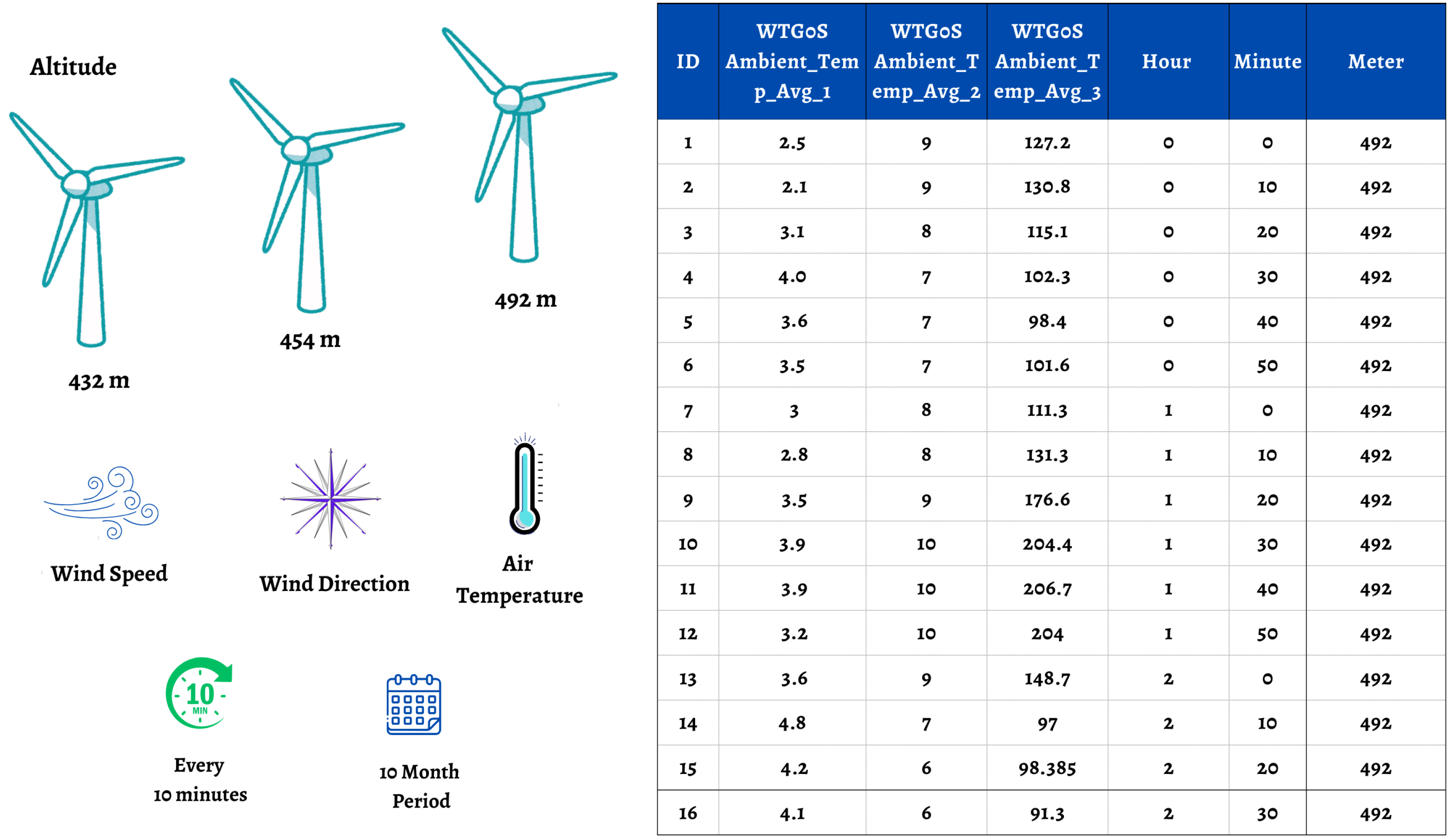
In this study, wind direction, wind speed, and air temperature values were collected separately for 432, 454, and 492 m from Yayladağ Sebenoba Location every 10 min for a period of 10 months starting from 1 January 2017 00:00:00. Some of these data are given in Figure 1. The reason why the data was not collected for a period of 12 months is due to maintenance work on the wind turbines in November and December of the year.

Then, the collected data were separated for each location and 3 different data sets were obtained.

Table 2. Datasets and properties.

Data Set	Number of Data	Parameters
Altitude 432 m	50.986	Wind_Speed, Wind_Temperature, Wind_Direction, Hour, Minute, Year, Day, Month, Year, Day_of_Week, Week_Day, Meter
Altitude 454 m	50.986	Wind_Speed, Wind_Temperature, Wind_Direction, Hour, Minute, Year, Day, Month, Year, Day_of_Week, Week_Day, Meter
Altitude 492 m	50.986	Wind_Speed, Wind_Temperature, Wind_Direction, Hour, Minute, Year, Day, Month, Year, Day_of_Week, Week_Day, Meter

shows the data sets and their properties.

2.2. Method

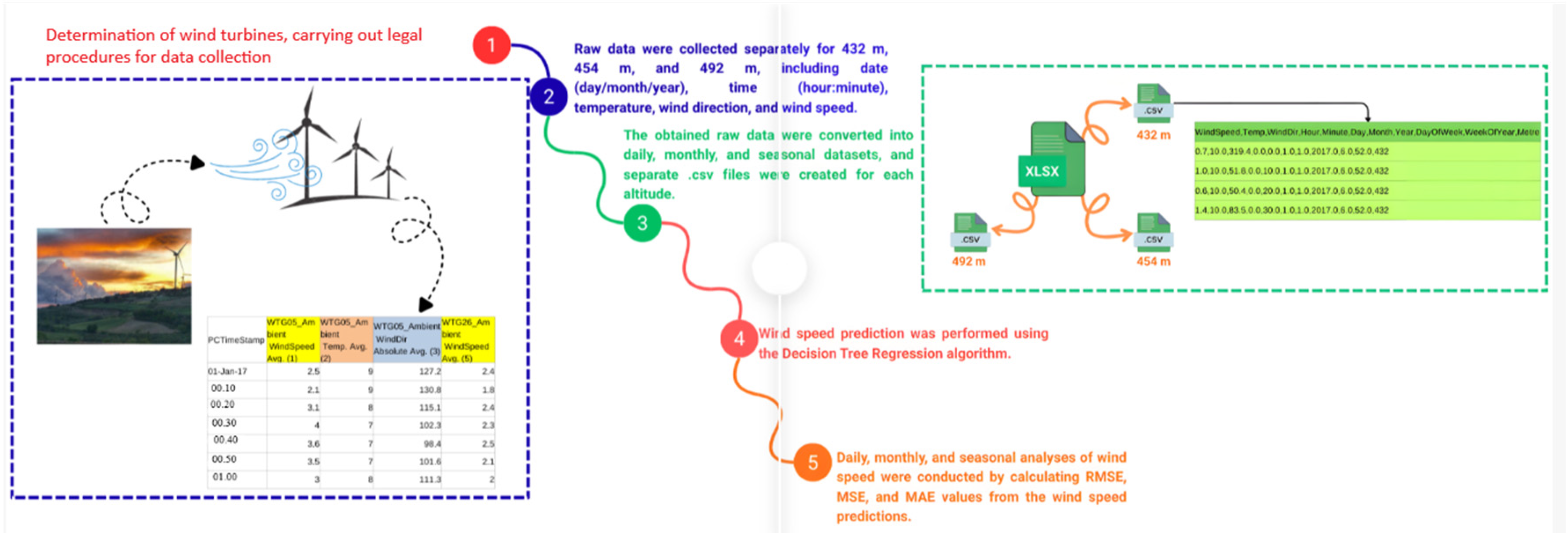
Figure 2 presents the flowchart of the applied methodology.

As shown in Figure 2, the proposed methodology consists of five main steps. First, after obtaining the necessary permissions and completing the legal procedures, data on date, wind direction, wind speed, and air temperature were collected over a long-term period of 10 months from wind turbines located at three different altitudes. Next, the collected data were separated according to the three altitudes, resulting in three distinct .csv files. From the date column in the format “day/month/year hour:minute” in each .csv file, new features were extracted, including hour, minute, day, month, year, day of the week, and week of the year, after which the original date column was removed. Following data preprocessing, the Decision Tree Regression algorithm was applied to predict daily, monthly, and seasonal wind speed using wind direction and air temperature as input variables. In the final step, the obtained results were analyzed.

The Decision Tree Regression method is a machine learning algorithm that tries to make predictions by dividing the data over the nodes in the tree structure. Each branch of the tree structure is a decision point. Each leaf node (terminal node) represents a prediction. Decision Tree constantly divides the data into two subgroups to make it homogeneous. It tests the independent variable at different points to find the best-split point. Then, at each node, the data is divided according to a certain rule, and thus the tree deepens as the data is divided into smaller pieces. At the end of the decision tree, at the points called leaves (terminal nodes), the average of the data, that is, the regression estimate, is created. These estimated values become the output of that node. In cases where Decision Trees are too deep, the depth of the decision tree is limited with hyperparameters such as maximum depth (max_depth) to prevent “overfitting”, that is, excessive learning and memorization.

Steps of Regression Method with Decision Tree

Regression analysis is a statistical method used to examine the relationships between variables. It is used especially to understand how a dependent variable (outcome or variable to be predicted) is related to independent variables (input or influencing factors). The main reasons why regression analysis is widely used can be listed as follows [30,31]:

• Making Predictions: Regression is a powerful tool for predicting future values from data.
• Understanding Casual Relationships: Regression can help measure the effect of a change in one variable on another variable.
• Modeling Complex Relationships: Especially in multiple regression models, more complex relationships and patterns can be analyzed using more than one independent variable.

Decision trees are a widely used algorithm for solving classification and regression problems in data mining and machine learning. Using a hierarchical structure, it divides the data into branches, which eventually reach decisions or predictions. Each branch divides the data into parts according to their features, so that classes or prediction values are obtained at the final leaf nodes. Decision trees are preferred scientific methods for the following reasons [32,33]:

• Understandability and Interpretability: Decision trees provide visually easy-to-understand structures.
• Less Data Preprocessing Requirement: Unlike some other machine learning methods, decision trees offer flexibility in working with missing data or categorical data.
• Speed and Computation Efficiency: Decision trees are widely used in working with large data sets because they can perform fast and efficient calculations.

The MSE, RMSE, MAE, and R² values calculated below were obtained using the wind speed estimates (y) obtained by decision tree regression. The wind speed estimated by decision tree regression is a numerical value. Therefore, it is very difficult for the obtained result to be exactly the same as the observed result. Instead, the target is for the estimated results to be very close to the observed result. Therefore, the target is for the MSE between the estimated and measured values to be as low as possible. The aim is to determine the lowest MSE in the fastest way by dividing the data with decision tree regression. The MSE is calculated by Equation (1) given below:

$$MSE={\displaystyle \frac{1}{n}}{\sum }_{i=1}^n{\left(y_{\dot{i}}-y^{\prime }\right)}^2$$

(1)

n = Number of Samples in Data

y_i = Actual value (target variable)

y′ = Estimated mean value (average found in each leaf)

• For each potential split point, the error in two subgroups is calculated. After dividing the split into two subgroups, the total error is calculated by Equation (2):

  $${MSE}_{Total}= {\displaystyle \frac{n_{left}}{n_{total}}}\times {MSE}_{left}+{\displaystyle \frac{n_{right}}{n_{total}}}\times {MSE}_{right}$$

  (2)

MSE_Total = Total error of all data after division

n_left ve n_right = Number of data split left and right

n_total = Total number of data

MSE_left ve MSE_right = MSE values in left and right split data

The algorithm calculates this total error for each split point and selects the split that gives the smallest error.

• RMSE, is the square root of the MSE value.
• MAE: In statistics, the MAE is a measure of the errors between observations (values) obtained for the same event. It can be used to compare predicted and measured values between samples of Y and X. MAE is calculated by dividing the absolute errors (e.g., Manhattan distance) by the sample size. Equation (3) shows how to calculate MAE.

  $$MAE={\displaystyle \frac{{\sum }_{i=1}^n\left|y_i-{y^{\prime }}_i\right|}{n}}={\displaystyle \frac{{\sum }_{i=1}^n\left|e_i\right|}{n}}$$

  (3)

e_i = i. absolute error, y_i = i. estimated value, y′_i = i. measured result

• The prediction at each leaf node is calculated by the average of the target variables at that leaf. If there are k data at a leaf node, the predicted value at the leaf is calculated by Equation (4):

  $${Y\prime }_{leaf}={\displaystyle \frac{1}{k}}\sum _{i=1}^k{Y}_i$$

  (4)

Y′_leaf = Predicted mean value at leaf node

k = Number of data in the leaf node

Y_i = Target variable values in the leaf node

• To prevent overfitting, i.e., excessive learning, depth is controlled with hyperparameters such as maximum depth (max_depth) or minimum number of samples in the leaf node (min_samples_leaf).
• The R-squared (R²) value is used to measure the performance of the decision tree. The R² value indicates how well the model explains the variance of the target variable. Equation (5) shows how the R² value is calculated.

  $$R^2=1-{\displaystyle \frac{\Sigma {(y_i-{y\prime }_i)}^2}{\Sigma {(y_i-z\prime )}^2}}$$

  (5)

y_i = Actual values

y′ = Values predicted by the model

z′ = Mean of target variable

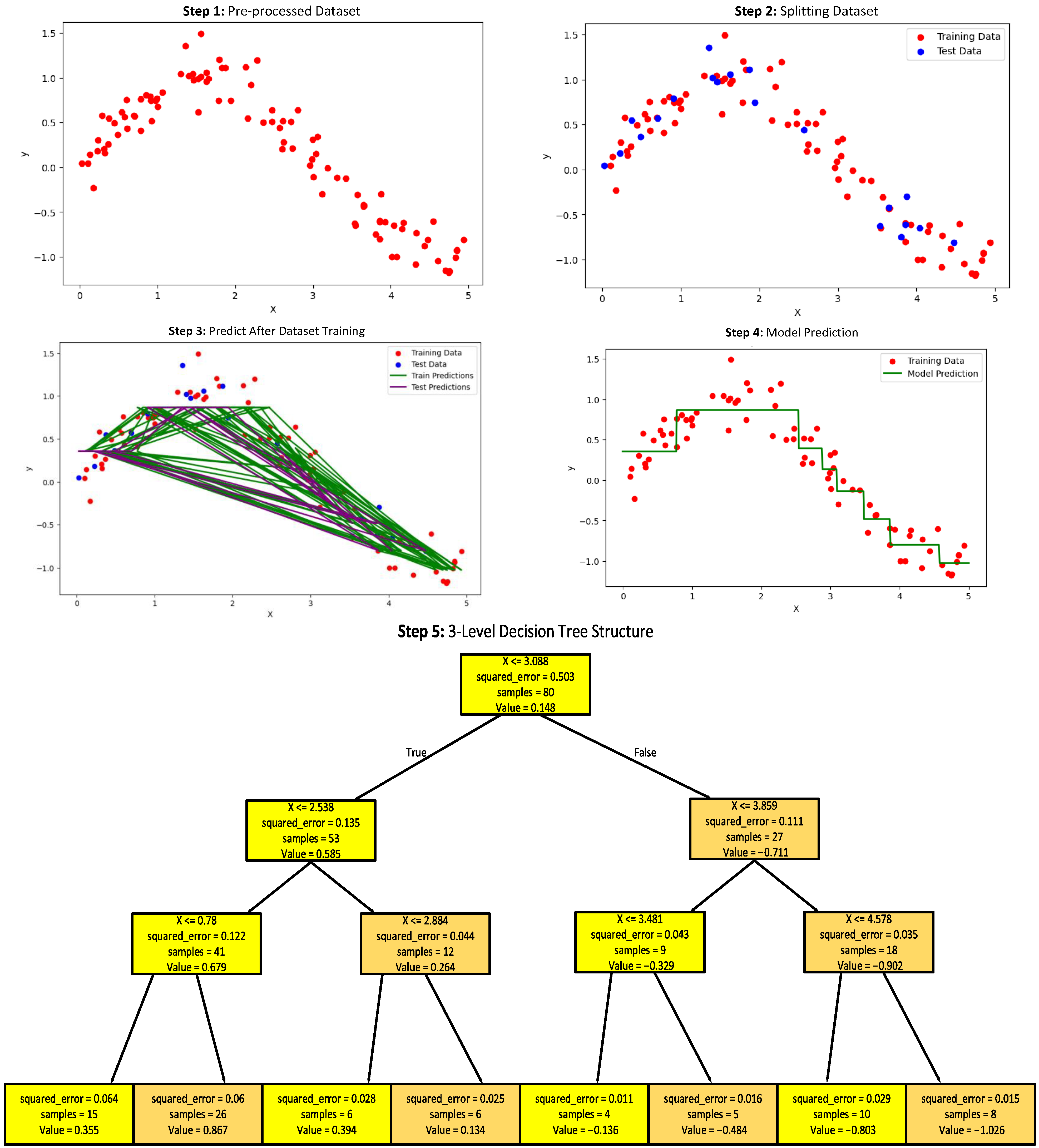
The visual explaining the working logic of the Regression method with a Decision Tree of 3 depths using randomly generated data is given in Figure 3.

Figure 3 illustrates the working logic of a regression approach based on a Decision Tree model with a maximum depth of three, using randomly generated data. The process is presented step by step to clearly demonstrate data preparation, model training, prediction, and the internal structure of the regression tree. In Step 1, the pre-processed dataset is shown, where the input variable x and the corresponding output variable y form a non-linear relationship with added noise. This step represents the initial data distribution after preprocessing. In Step 2, the dataset is divided into training and test sets. The training samples are used to build the regression model, while the test samples are reserved for evaluating the generalization capability of the trained model. Both subsets preserve the overall trend of the original data. Step 3 demonstrates the prediction process after training the Decision Tree regression model. The predicted outputs for both training and test data are visualized, highlighting how the model approximates the underlying data distribution. The piecewise nature of the predictions reflects the rule-based structure of the Decision Tree. In Step 4, the model predictions are overlaid on the training data. The resulting regression curve exhibits a step-like behavior, which is characteristic of Decision Tree regression. Each flat segment corresponds to a leaf node, where predictions are obtained by averaging the target values within that region. Finally, Step 5 presents the internal structure of the trained Decision Tree with a depth of three. Each node displays the splitting condition, squared error, number of samples, and predicted value. The hierarchical structure illustrates how the input space is recursively partitioned into smaller regions to minimize the prediction error.

In this study, a Decision Tree Regression model was used for wind speed estimation. The model was structured and trained in the MATLAB R2025b Regression Learner Toolbox environment. Mean Squared Error (MSE) was used as the splitting criterion in the decision tree. To prevent overfitting, the maximum depth of the decision tree was limited, and the minimum number of samples required at each leaf node was determined. During model training, the most suitable splits were automatically selected based on error reduction.

3. Experimental Results and Discussion

In this study, MATLAB Regression Learner Toolbox was used to obtain regression results. This Toolbox was run on a computer with a 64-bit Windows operating system, Intel i7 processor, and 32 GB memory. Decision Tree and Regression method was preferred for regression (Figure 3).

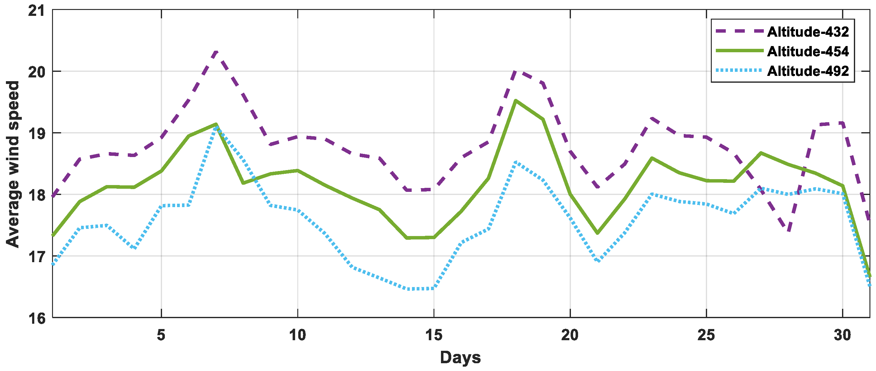
The daily average wind speed graph is given in Figure 4. While creating this graph, the wind speed values on the first day of each month were averaged among themselves and the wind speed values on the second day were calculated. When the given graph is examined, it is seen that the wind speeds up as the altitude decreases daily.

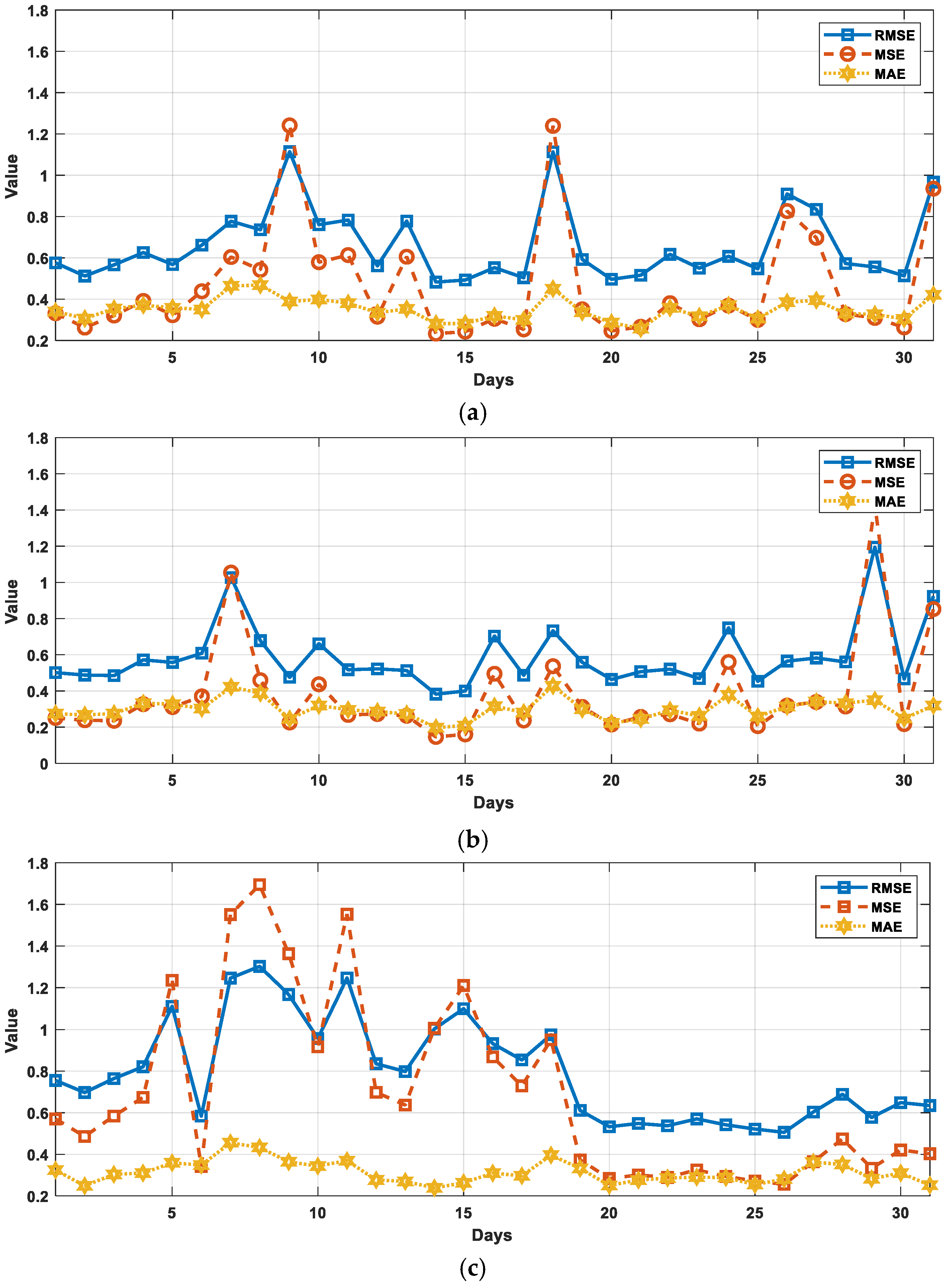
The daily wind speed detection results graph is given in Figure 5. When the prediction graph in Figure 5 is compared with the actual values in Figure 4, it is seen that the detection results are more accurate at 432 altitude and the detection deviates from the facts as the altitude increases.

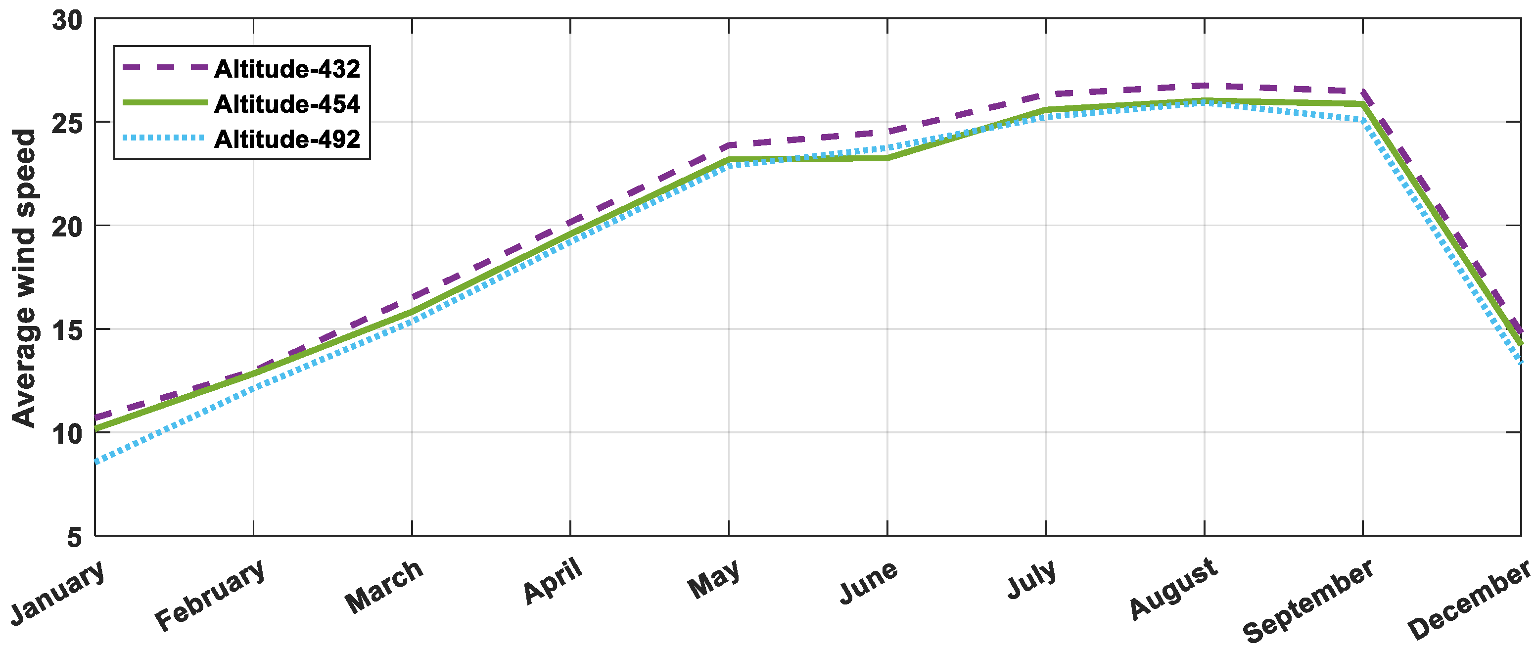
The monthly average wind speed graph is given in Figure 6. This graph was created by taking the average of the wind speed values on a monthly basis for each month. When the graph is examined, it is seen that the wind speed is low in December, January, and February, and generally increases from March, April, and May to September.

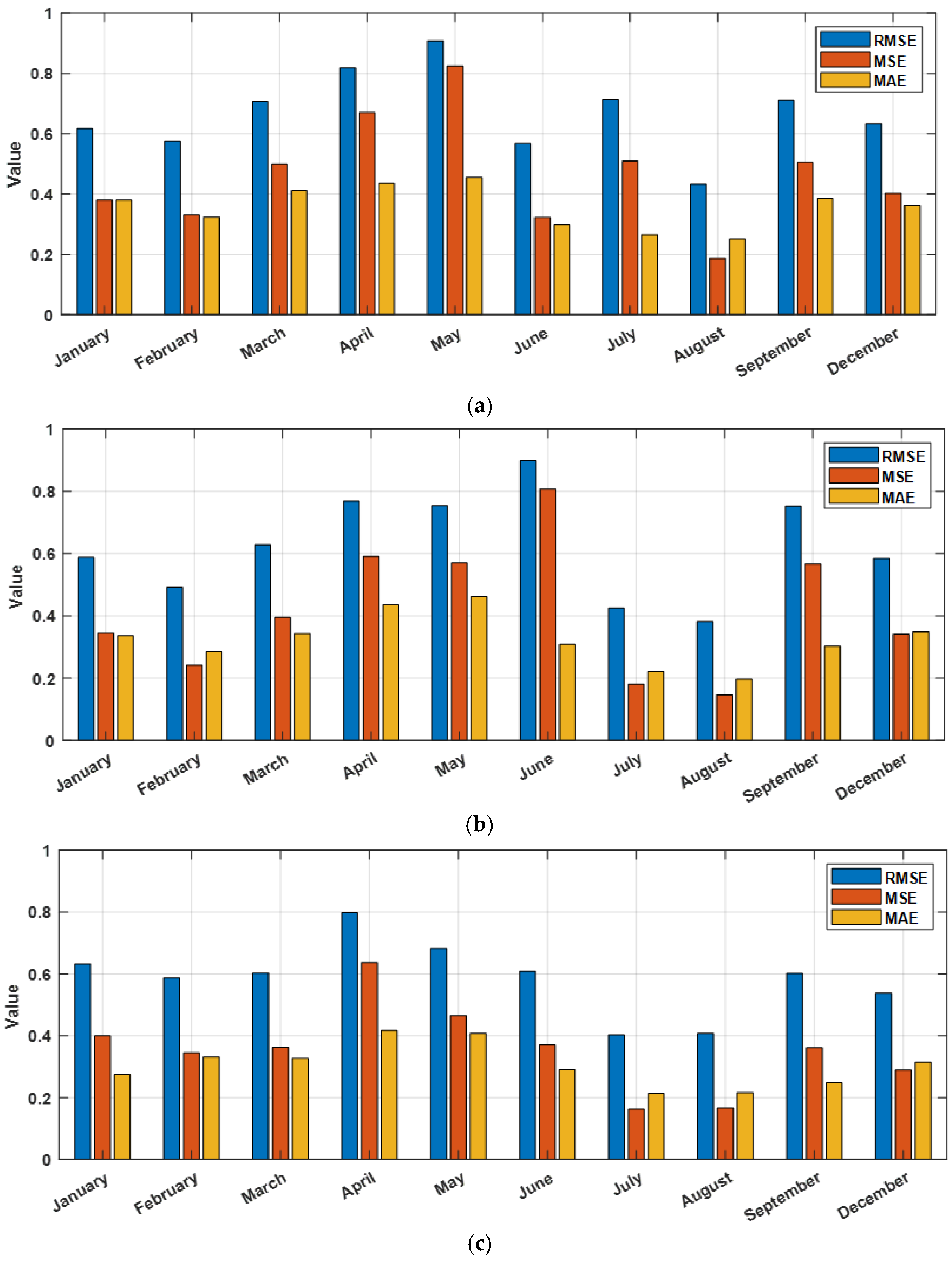
Monthly wind speed determination results are given in Figure 7. When these results are compared with the actual values in Figure 5, it is seen that the wind speed is determined more accurately for each altitude, especially in July and August.

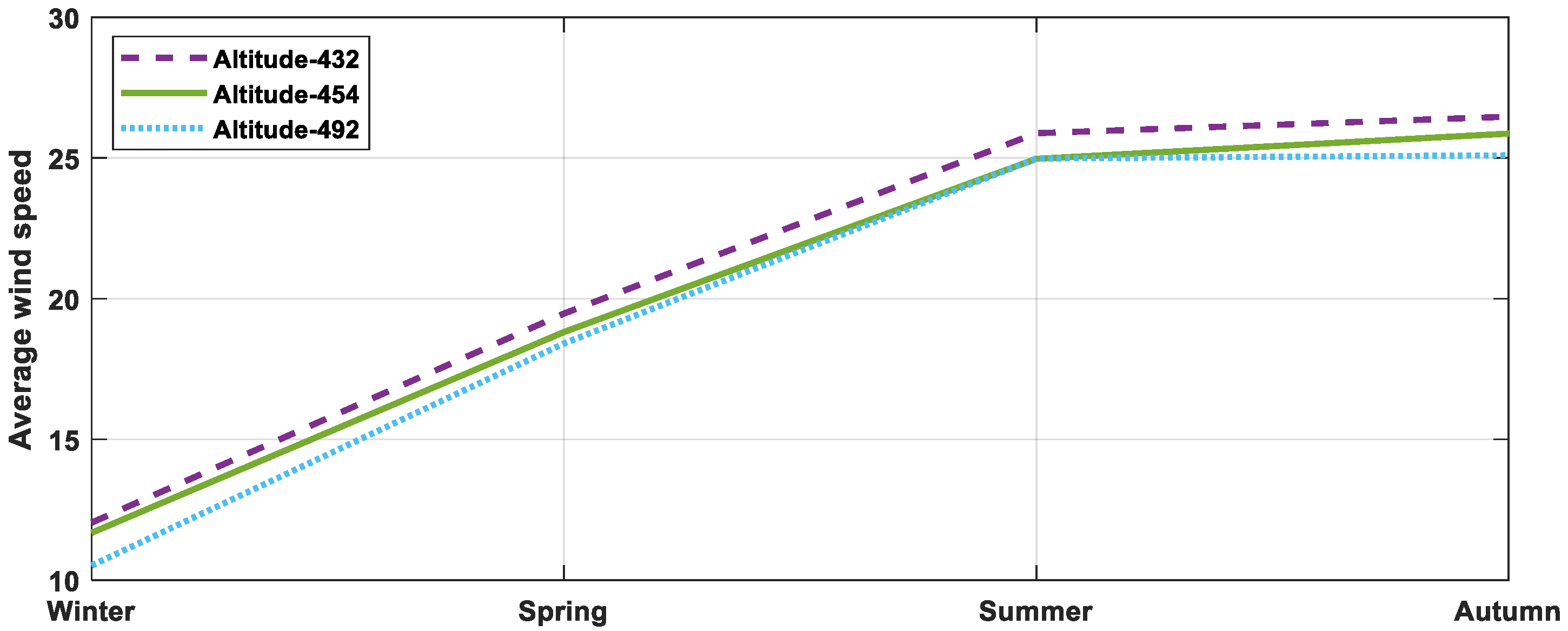
The seasonal average wind speed graph is given in Figure 8. According to this graph, it is seen that the wind speed is low in the winter season for each altitude and increases in the spring season. From this, it can be concluded that the wind speed decreases as the weather becomes colder and the wind speed increases as the air temperature increases.

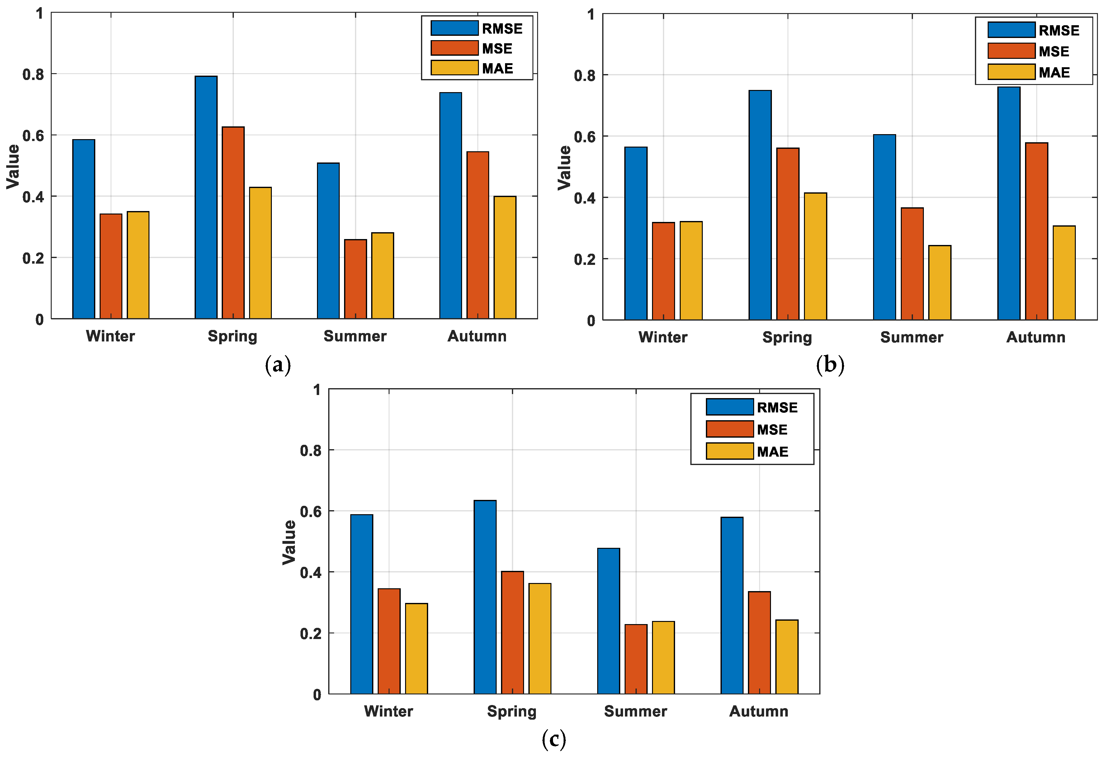
The seasonal wind speed detection results graph is given in Figure 9. When the given detection graph is compared with the real data in Figure 8, it is seen that the summer season especially is detected more accurately for each altitude.

In

Table 3. General results after training.

Parameters	Altitude 432	Altitude 454	Altitude 492	Altitude All
RMSE	0.64917	0.66629	0.59954	0.60188
R-Squared	0.99	0.99	0.99	0.99
MSE	0.42143	0.44394	0.35945	0.36226
MAE	0.36573	0.33447	0.31004	0.35941
Training Time	7.2809 s	5.8373 s	5.8281 s	20.645 s

, for each altitude and for all altitudes (Altitude All) combined and collective training is performed, each training result and training time are given separately. There is no distinction between day, month, and season in the training performed here (Day, month, and season values are also among the independent variables used to estimate wind speed.). When the given table is examined; it is seen that the results of altitude 492, which has the lowest performance values and training time, are the best. In addition, it is seen that there is not much change in the performance values compared to the others from the results obtained by combining all altitudes and even better results are given compared to altitudes 432 and 454, but the training time is much longer than the others.

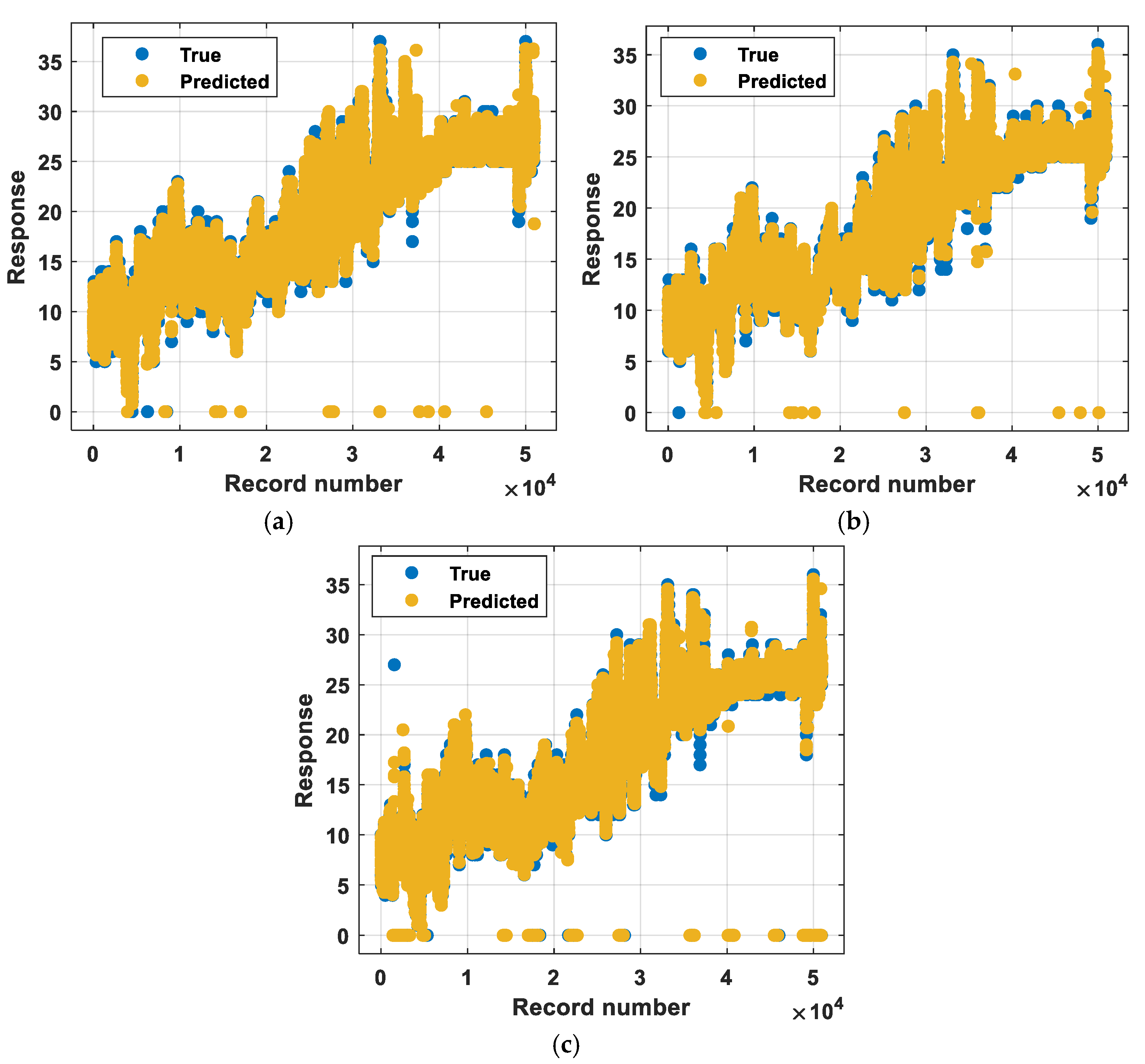
Figure 10 compares the actual and estimated wind speeds for each altitude. Blue dots represent actual values, and yellow dots represent estimated values. When the given graphs are examined, it is seen that the estimated values are generally quite close to the actual values. This shows that the models have a successful performance. In particular, all three graphs indicate that the models have a consistent performance in large data sets. It is also observed that in the model created at 492 altitudes, the actual and estimated values are closer to each other and perform better than the others.

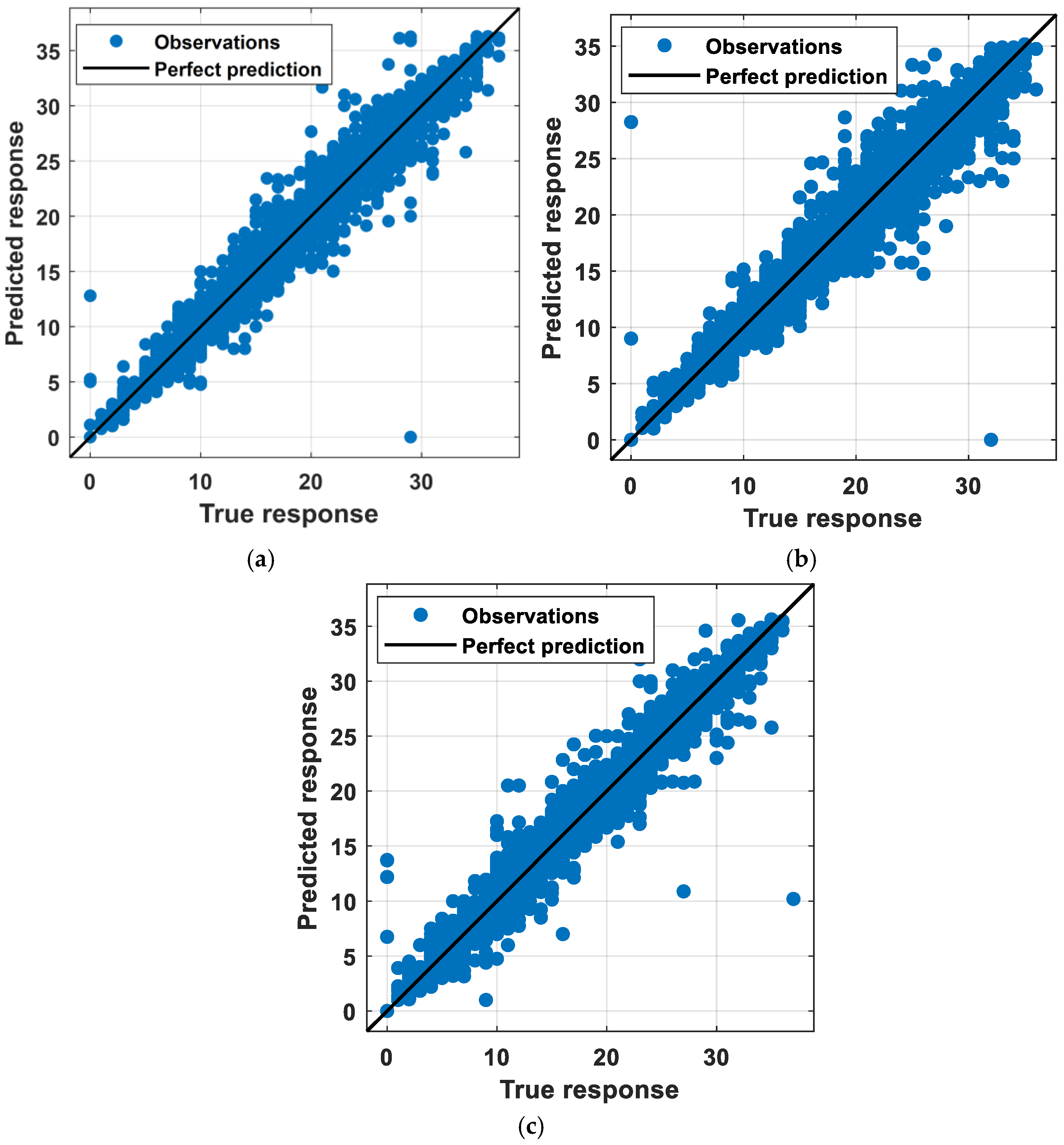
In Figure 11, the perfect prediction line graph, which is a reference line representing the situation where the model’s predictions are completely accurate for each altitude, is given. The closer the blue points, that is, the prediction values, are to this line, the more accurate the prediction is. Based on this information, it can be seen that although there are deviations at some points, the predictions at altitude 492 are closer to the line and more accurate.

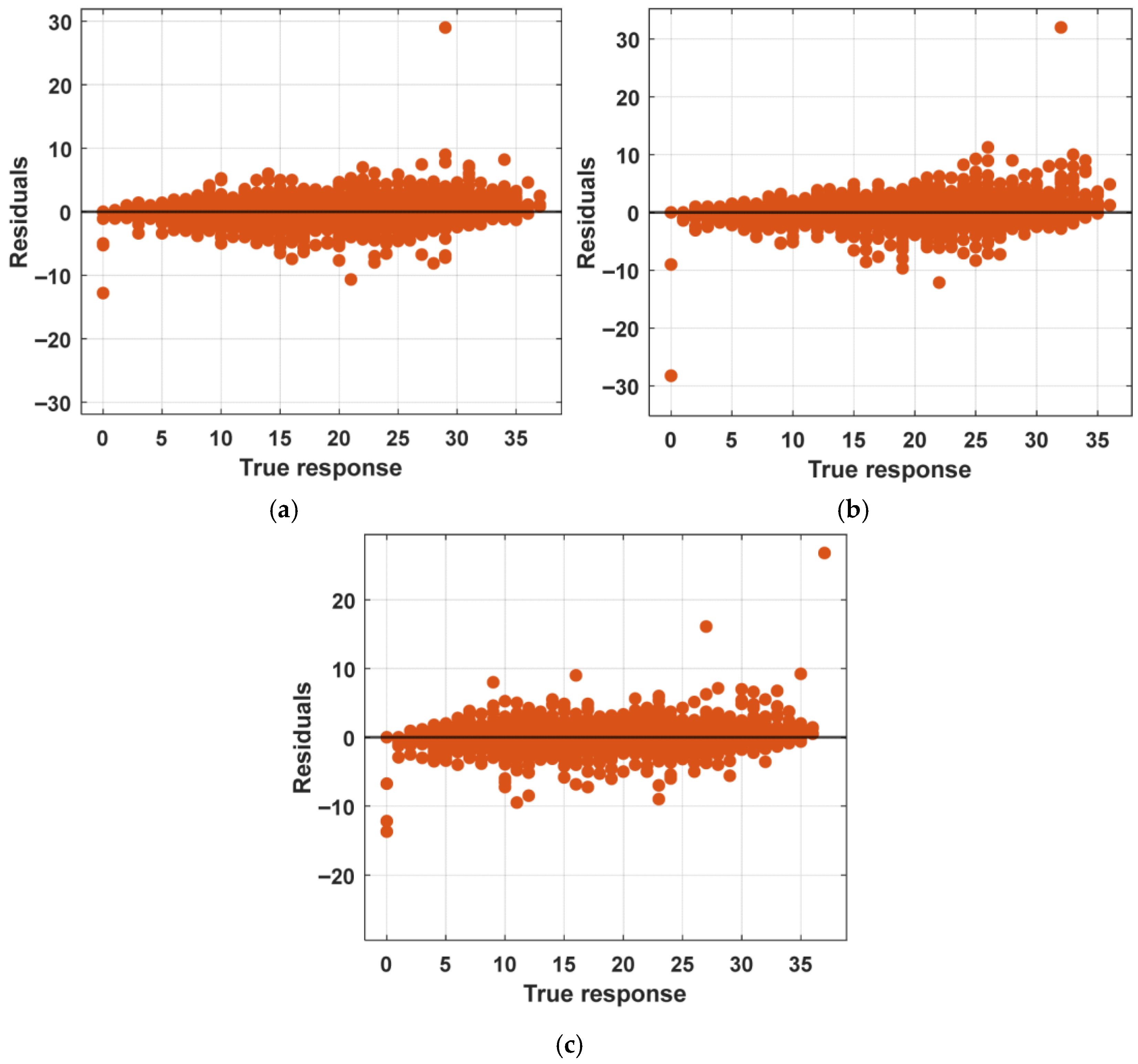
Figure 12 shows the “Residuals/True Response” graphs for each altitude. Residuals represent the difference between the value predicted by the model and the actual value. True Response is the actual values that the model is trying to predict. In an ideal model, residual values should be zero or very close to zero. If the residuals values are different from zero, this means that the model is making incorrect predictions. If the residuals values show a certain trend or pattern, this indicates that the model is making incorrect predictions. When this information is taken into consideration and the graphs given are examined, it is seen that the altitude of 492 has a more uniform and balanced distribution compared to other altitudes. Here, the residual values are generally distributed homogeneously around 0 and do not show a significant trend. This means that the model is making more balanced and consistent predictions at this altitude.

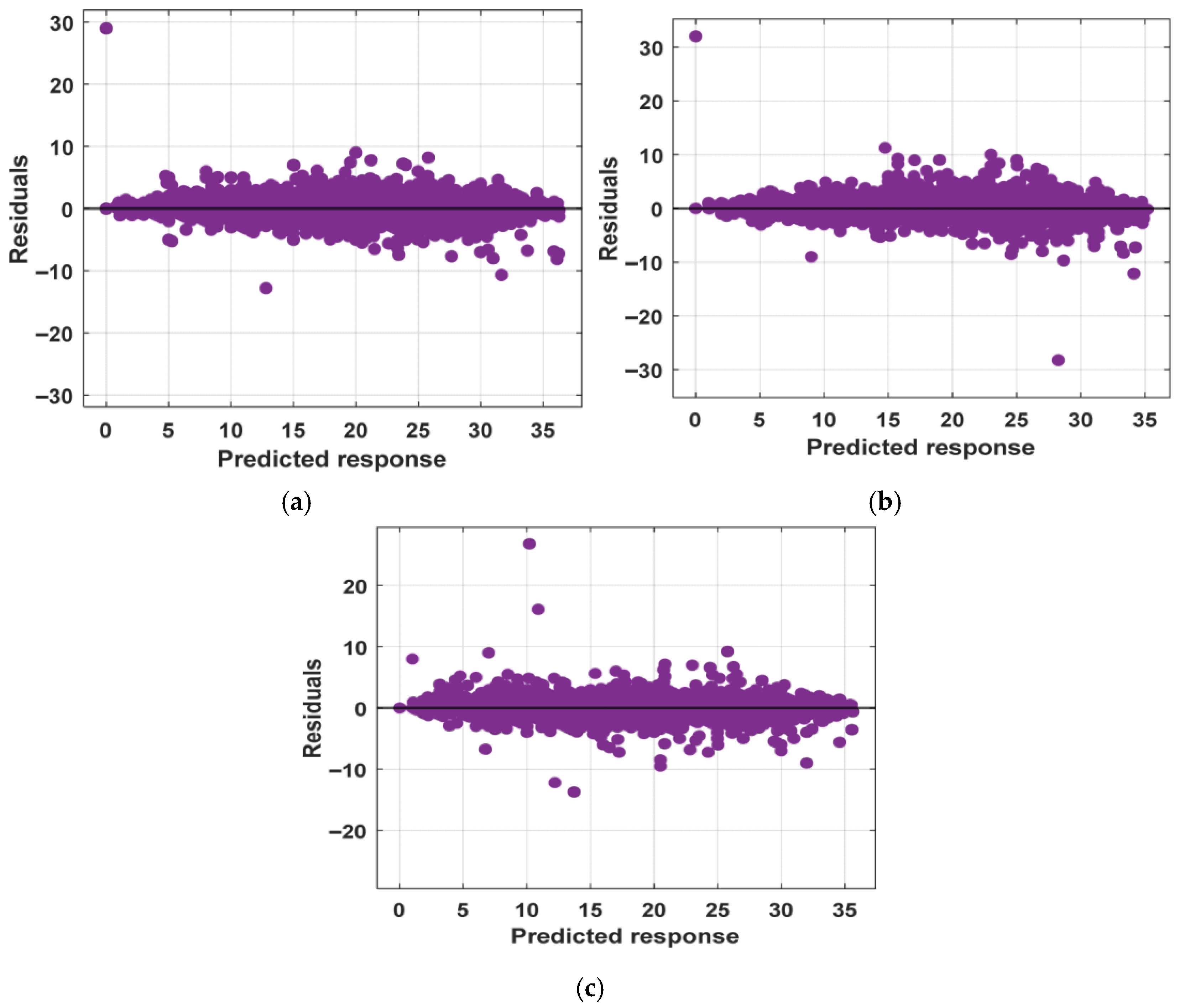
Figure 13 shows the “Residuals/Predicted Response” graphs for each altitude. The predicted response value represents the values predicted by the model. In a good model, residual values should generally be symmetrically distributed around 0 and randomly distributed throughout the predicted response. If this distribution grows and shrinks depending on the predicted values, for example, if it takes the shape of a funnel, this indicates that the model makes more errors in certain data regions. When the graphs are examined after all this information, it is observed that the residual values for all three altitudes are concentrated around 0 and do not have any pattern. This shows that the performance of the model is generally satisfactory and that there is no systematic error. It was observed that the errors increased at some data points. However, these increases remain at lower levels for the 492 altitudes compared to other altitudes. This shows that the model can produce more stable results for the 492 altitudes.

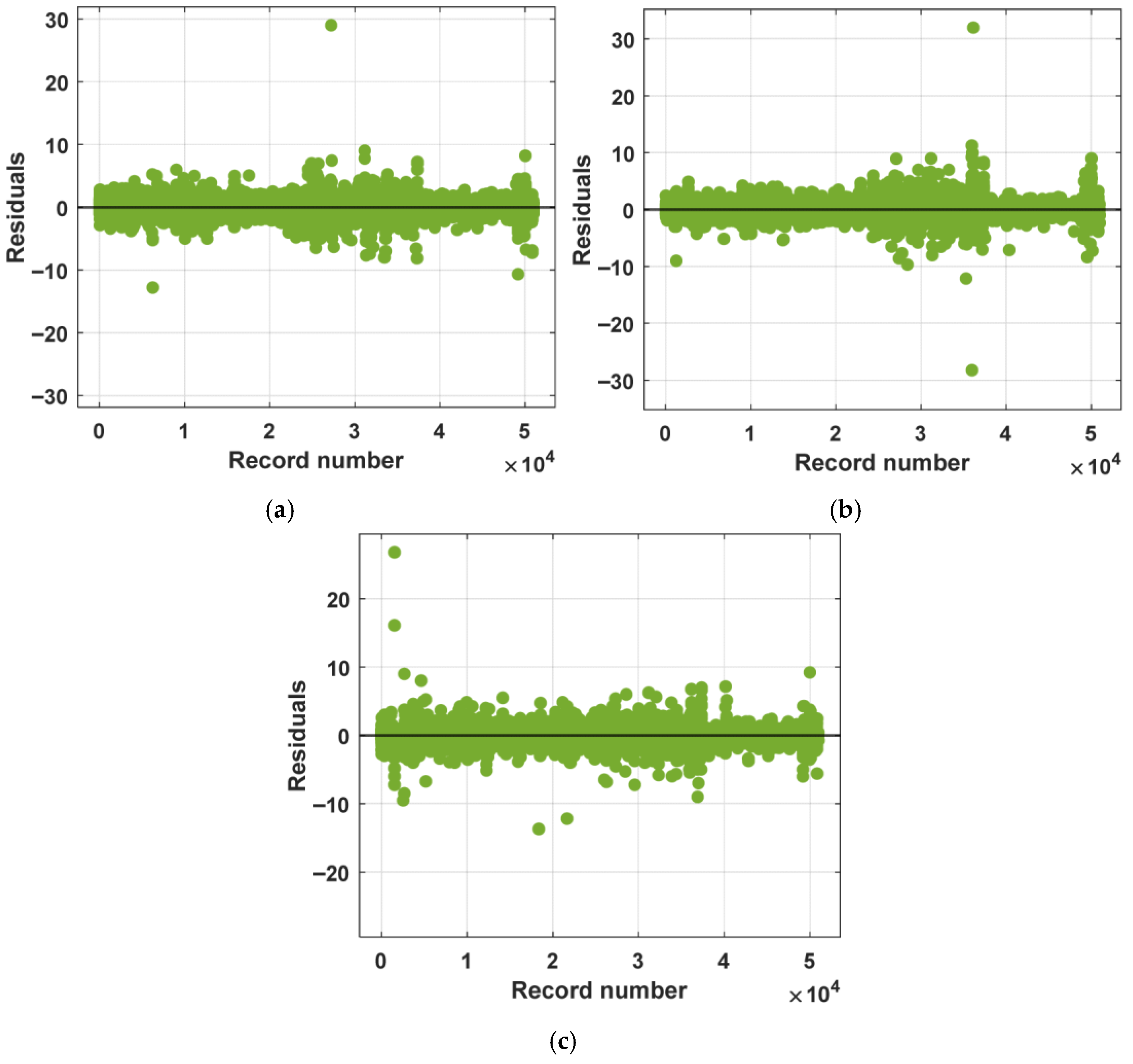
Figure 14 shows the “Residuals/Record Number” graphs for each altitude. When the graphs are examined, it is seen that the residual values do not show a systematic pattern and are generally randomly distributed. This situation shows that the model’s prediction errors do not increase over time. However, for some residual values, it is seen that the model makes larger errors at certain data points. These increases remain at lower levels for the 492 altitudes compared to other altitudes. This shows that the model can produce more stable results for the 492 altitudes. All graphs presented in Figure 10, Figure 11, Figure 12, Figure 13 and Figure 14 are consistent with the quantitative results reported in

Table 4. Daily, monthly, and seasonal wind speed predictions and RMSE results.

	Parameters	Statistics	Altitude 432	Altitude 454	Altitude 492
RMSE	Daily	Mean	0.6595	0.5910	0.7958
		Std	0.1762	0.1795	0.2465
	Monthly	Mean	0.6684	0.6276	0.5860
		Std	0.1350	0.1660	0.1179
	Seasonal	Mean	0.6554	0.6693	0.5690
		Std	0.1316	0.0997	0.0659
Wind Speed	Daily	Mean	18.7696	18.1589	17.5792
		Std	0.6651	0.6044	0.6484
	Monthly	Mean	20.3049	19.6529	19.1412
		Std	6.1224	5.9678	6.3555
	Seasonal	Mean	20.9660	20.3341	19.7526
		Std	6.7412	6.5647	6.9034

. However, the performance varies depending on the temporal resolution. While the altitude of 432 m yields lower RMSE values on a daily basis, the altitude of 492 m demonstrates superior performance for monthly and seasonal predictions. Therefore, no single altitude can be considered universally optimal across all temporal scales.

Table 4 shows the values of the average and standard deviations of the “Daily, Monthly, and Seasonal” wind speeds for each altitude, along with the RMSE performance values at the end of the training. According to the information provided in Table 4; the best RMSE (0.5910) value was obtained at the altitude of 432, which had the highest average wind speed value on a “Daily” basis (18.7696). The worst RMSE (0.7958) value was observed at the altitude of 492, which had the lowest average wind speed value (17.5792). On a “daily” basis, the best RMSE (0.1762) value and the highest wind speed standard deviation value (0.6651) are seen at 432 altitudes. The worst RMSE (0.2465) value is at altitude 492, and the lowest wind speed standard deviation value (0.6044) is at altitude 454. The best RMSE (0.5860) value is obtained at altitude 492, where the average wind speed value is the lowest on a “monthly” basis (19.1412). The worst RMSE value (0.6684) was observed at altitude 432, which has the highest average wind speed value (20.3049). On a “monthly” basis, the best RMSE (0.1179) value was obtained at 492 altitudes, which had the highest wind speed standard deviation value (6.3555). The worst RMSE (0.1660) value was observed at 454 altitudes, which had the lowest wind speed standard deviation value (5.9678). The best RMSE (0.5690) value was obtained at 492 altitude, where the average wind speed value was the lowest on a “seasonal” basis (19.7526). The worst RMSE (0.6693) value was observed at altitude 454, and the highest average wind speed value (20.9660) was observed at altitude 432. The best RMSE (0.0659) value was obtained at altitude 492, where the highest wind speed standard deviation value (6.9034) was obtained on a “seasonal” basis. The worst RMSE (0.1316) value was observed at altitude 432, and the lowest wind speed standard deviation value (6.5647) was observed at altitude 454.

4. Conclusions

If the obtained experimental results are evaluated comprehensively, it is observed that prediction performance varies depending on both altitude and temporal resolution. The station located at the highest altitude (492 m) yields the lowest RMSE values for monthly and seasonal predictions, and this performance is supported by the corresponding standard deviation values. However, daily forecast results show that lower altitudes may be advantageous. Specifically, an altitude of 432 m produces lower daily RMSE values, while an altitude of 454 m shows lower standard deviation values in certain situations. Interpreting these results, it shows that high-altitude stations generally provide better forecasts over longer temporal scales, and lower altitudes may be preferred in situations where short-term accuracy or higher wind speed values are more important. Although the datasets used in this study contain a limited number of parameters, the proposed method states that reliable and accurate wind speed forecasts can be obtained using combined statistical features. It is necessary to mention the limitations of the Decision Tree model used in our study. Decision Trees have a high fit behavior and are designed to clearly capture temporal constraints in wind speed time series. Additionally, lagged wind speed features, which are important in wind forecasting, were not included in the current model. Thanks to this method, it was determined that the analysis of altitude-related effects is more understandable, independent of the confounding effects of complex temporal architectures. In practical applications, high-altitude stations may be preferred when minimizing RMSE is the primary goal, while lower-altitude stations may be considered in scenarios where higher wind speed values are more critical. Our future work will focus on determining the optimal balance between wind speed and forecast error using multi-objective meta-heuristic optimization techniques. Furthermore, we will explore the integration of lag features and more advanced temporal models such as ensemble tree methods and recurrent neural networks to further improve forecast performance. Future work will expand on this study by integrating temporal models, including LSTM-based architectures, as well as ensemble learning methods such as Random Forest, Gradient Boosting, and XGBoost, and will examine the balance between accuracy, interpretability, and computational cost by conducting a comprehensive performance comparison.

References

1. Altan, A.; Karasu, S.; Zio, E. A new hybrid model for wind speed forecasting combining long short-term memory neural network, decomposition methods and grey wolf optimizer. Appl. Soft Comput. 2021, 100, 106996. [Google Scholar] [CrossRef]
2. Karasu, S.; Altan, A.; Saraç, Z.; Hacıoğlu, R. Estimation of Fast Varied Wind Speed Based on Narx Neural Network by Using Curve Fitting. Int. J. Energy Appl. Technol. 2017, 4, 137–146. [Google Scholar]
3. Karasu, S.; Altan, A.; Saraç, Z.; Hacioglu, R. Estimation of Wind Speed by using Regression Learners with Different Filtering Methods. In Proceedings of the First International Conference on Energy Systems Engineering (ICESE’17), Safranbolu, Turkey, 2–4 November 2017. [Google Scholar]
4. Karasu, S.; Altan, A.; Sarac, Z.; Hacioglu, R. Prediction of wind speed with non-linear autoregressive (NAR) neural networks. In Proceedings of the 2017 25th Signal Processing and Communications Applications Conference (SIU), Antalya, Turkey, 15–18 May 2017. [Google Scholar] [CrossRef]
5. Wang, J.; Zhang, W.; Wang, J.; Han, T.; Kong, L. A novel hybrid approach for wind speed prediction. Inf. Sci. 2014, 273, 304–318. [Google Scholar] [CrossRef]
6. Bouzgou, H.; Benoudjit, N. Multiple architecture system for wind speed prediction. Appl. Energy 2011, 88, 2463–2471. [Google Scholar] [CrossRef]
7. Hu, J.; Wang, J.; Ma, K. A hybrid technique for short-term wind speed prediction. Energy 2015, 81, 563–574. [Google Scholar] [CrossRef]
8. Mohandes, M.A.; Halawani, T.O.; Rehman, S.; Hussain, A.A. Support vector machines for wind speed prediction. Renew. Energy 2004, 29, 939–947. [Google Scholar] [CrossRef]
9. Filik, Ü.B.; Filik, T. Wind Speed Prediction Using Artificial Neural Networks Based on Multiple Local Measurements in Eskisehir. Energy Procedia 2017, 107, 264–269. [Google Scholar] [CrossRef]
10. Zhu, Q.; Chen, J.; Zhu, L.; Duan, X.; Liu, Y. Wind speed prediction with spatio-temporal correlation: A deep learning approach. Energies 2018, 11, 705. [Google Scholar] [CrossRef]
11. Rehman, S. Long-term wind speed analysis and detection of its trends using Mann-Kendall test and linear regression method. Arab. J. Sci. Eng. 2013, 38, 421–437. [Google Scholar] [CrossRef]
12. Deng, Y.-C.; Tang, X.-H.; Zhou, Z.-Y.; Yang, Y.; Niu, F. Application of machine learning algorithms in wind power: A review. Energy Sources Part A Recover. Util. Environ. Eff. 2021, 47, 4451–4471. [Google Scholar] [CrossRef]
13. Yağmur, E.Ç.; Yağmur, S. Rüzgar Gücü Tahmininde Genetik Algoritma ile Öznitelik Seçimi. Afyon Kocatepe Üniv. Fen Mühendis. Bilim. Derg. 2022, 22, 1028–1040. [Google Scholar] [CrossRef]
14. Park, S.; Jung, S.; Lee, J.; Hur, J. A Short-Term Forecasting of Wind Power Outputs Based on Gradient Boosting Regression Tree Algorithms. Energies 2023, 16, 1132. [Google Scholar] [CrossRef]
15. Oyucu, S.; Aksöz, A. Integrating Machine Learning and MLOps for Wind Energy Forecasting: A Comparative Analysis and Optimization Study on Türkiye’s Wind Data. Appl. Sci. 2024, 14, 3725. [Google Scholar] [CrossRef]
16. Magesh, T.; Franklin, F.S.; Santhi, P.S.; Thiyagesan, M. Machine Learning-Driven Wind Energy Forecasting for Sustainable Development. MATEC Web Conf. 2024, 393, 02003. [Google Scholar] [CrossRef]
17. Tümse, S.; İlhan, A.; Bilgili, M.; Şahin, B. Estimation of wind turbine output power using soft computing models. Energy Sources Part A Recover. Util. Environ. Eff. 2022, 44, 3757–3786. [Google Scholar] [CrossRef]
18. Bilgili, M.; Ilhan, A.; Tumse, S.; Sahin, B. Machine learning approaches in predicting the wind power output and turbine rotational speed in a wind farm. Energy Sources Part A Recover. Util. Environ. Eff. 2024, 46, 12084–12110. [Google Scholar] [CrossRef]
19. Anushalini, T.; Revathi, B.S. Role of Machine Learning Algorithms for Wind Power Generation Prediction in Renewable Energy Management. IETE J. Res. 2024, 70, 4319–4332. [Google Scholar] [CrossRef]
20. Amer, T.S.; Arab, A.; Galal, A.A. On the influence of an energy harvesting device on a dynamical system. J. Low Freq. Noise Vib. Act. Control. 2024, 43, 669–705. [Google Scholar] [CrossRef]
21. Amer, T.S.; Wahba, A.M.; Abolila, A.F.; Galal, A.A. Optimizing stability and characteristics of a vibrating rigid body pendulum with energy harvesting device. J. Low Freq. Noise Vib. Act. Control. 2025, 44, 893–937. [Google Scholar] [CrossRef]
22. Li, Y.; Shen, X. A novel wind speed-sensing methodology for wind turbines based on digital twin technology. IEEE Trans. Instrum. Meas. 2021, 71, 2503213. [Google Scholar] [CrossRef]
23. Li, Y.; Shen, X.; Zhou, C. Dynamic multi-turbines spatiotemporal correlation model enabled digital twin technology for real-time wind speed prediction. Renew. Energy 2023, 203, 841–853. [Google Scholar] [CrossRef]
24. Sierra-García, J.E.; Santos, M. Improving wind turbine pitch control by effective wind neuro-estimators. IEEE Access 2021, 9, 10413–10425. [Google Scholar] [CrossRef]
25. Elkelawy, M.; Atta, Z.A.; Seleem, H. Technological advances, efficiency optimization, and challenges in wind power plants: A comprehensive review. Pharos Eng. Sci. J. 2024, 1, 57–65. [Google Scholar] [CrossRef]
26. Mayilsamy, G.; Palanimuthu, K.; Venkateswaran, R.; Antonysamy, R.P.; Lee, S.R.; Song, D.; Joo, Y.H. A review of state estimation techniques for Grid-Connected PMSG-Based wind turbine systems. Energies 2023, 16, 634. [Google Scholar] [CrossRef]
27. Barambones, O.; Cortajarena, J.A.; Calvo, I.; de Durana, J.M.G.; Alkorta, P.; Karami-Mollaee, A. Real time observer and control scheme for a wind turbine system based on a high order sliding modes. J. Frankl. Inst. 2021, 358, 5795–5819. [Google Scholar] [CrossRef]
28. Wu, T.; Ling, Q. STELLM: Spatio-temporal enhanced pre-trained large language model for wind speed forecasting. Appl. Energy 2024, 375, 124034. [Google Scholar] [CrossRef]
29. Couto, A.; Estanqueiro, A. Enhancing wind power forecast accuracy using the weather research and forecasting numerical model-based features and artificial neuronal networks. Renew. Energy 2022, 201, 1076–1085. [Google Scholar] [CrossRef]
30. Rimmer, R.; Draper, N.R.; Smith, H. Applied Regression Analysis. J. R. Stat. Soc. 1968, 18, 69. [Google Scholar] [CrossRef]
31. Myers, R.H.; Montgomery, D.C.; Vining, G.G.; Robinson, T.J. Generalized Linear Models: With Applications in Engineering and the Sciences, 2nd ed.; Wiley: Hoboken, NJ, USA, 2012. [Google Scholar] [CrossRef]
32. Breiman, L.; Friedman, J.H.; Olshen, R.A.; Stone, C.J. Classification and Regression Trees; CRC: Boca Raton, FL, USA, 2017. [Google Scholar]
33. Salzberg, S.L. C4.5: Programs for Machine Learning by J. Ross Quinlan, Morgan Kaufmann Publishers, Inc., 1993. Mach. Learn. 1994, 16, 235–240. [Google Scholar] [CrossRef]
Figure 1. Sample data collected in the study.
Sustainability 18 01067 g001
Figure 2. General application steps of the method.
Sustainability 18 01067 g002
Figure 3. Working logic of regression method with Decision Tree having 3 depths with randomly generated data.
Sustainability 18 01067 g003
Figure 4. Daily average wind speed graph.
Sustainability 18 01067 g004
Figure 5. Daily analysis: (a) Altitude 432, (b) Altitude 454, (c) Altitude 492.
Sustainability 18 01067 g005
Figure 6. Monthly average wind speed graph.
Sustainability 18 01067 g006
Figure 7. Monthly analysis (a) Altitude 432, (b) Altitude 454, (c) Altitude 492.
Sustainability 18 01067 g007
Figure 8. Seasonal average wind speed graph.
Sustainability 18 01067 g008
Figure 9. Seasonal analysis (a) Altitude 432, (b) Altitude 454, (c) Altitude 492.
Sustainability 18 01067 g009
Figure 10. (a) Altitude 432, (b) Altitude 454, (c) Altitude 492.
Sustainability 18 01067 g010
Figure 11. (a) Altitude 432, (b) Altitude 454, (c) Altitude 492.
Sustainability 18 01067 g011
Figure 12. (a) Altitude 432, (b) Altitude 454, (c) Altitude 492.
Sustainability 18 01067 g012
Figure 13. (a) Altitude 432, (b) Altitude 454, (c) Altitude 492.
Sustainability 18 01067 g013
Figure 14. (a) Altitude 432, (b) Altitude 454, (c) Altitude 492.
Sustainability 18 01067 g014