Multi-Objective Optimization of Relief-Well Dewatering for Canals Under High Groundwater Levels Using NSGA-II and Entropy-Weighted TOPSIS

Abstract

High groundwater levels can generate excessive uplift pressure beneath canal linings, causing heaving, cracking, and sliding failure. This study developed a multi-objective framework for relief-well dewatering design in a damaged reach of the headrace canal at the HLJ Hydropower Station. A three-dimensional finite-element seepage model, validated using field-monitoring data under a cross-condition validation framework, was combined with a Box–Behnken design and response surface methodology to quantify the effects of relief-well location, spacing, and depth to the pumping control water level on the relative uplift pressure head and pumping rate. NSGA-II was used to generate Pareto-optimal solutions considering hydraulic safety, number of relief wells, and total pumping demand. Hydraulic conductivity sensitivity analysis showed that the sand–gravel layer had the greatest influence on uplift pressure. The maximum adverse head increment of 0.0047 m was adopted as a hydraulic-conductivity sensitivity margin, resulting in a sensitivity-adjusted screening threshold of 0.2253 m. Entropy-weighted TOPSIS identified a compromise design with a well-to-canal-edge distance of 1.95 m, a spacing of 38.8 m, a depth to the pumping control water level of 8.36 m, and 32 relief wells. Monte Carlo weight sensitivity analysis indicated that the TOPSIS ranking was stable under moderate weight variations but became more sensitive at larger perturbations. Finite-element verification yielded a relative uplift pressure head of 0.2232 m and a total pumping rate of 0.3462 m³/s, with the verified head remaining below the sensitivity-adjusted screening threshold and the selected scheme providing a reasonable balance among uplift-pressure control, construction scale, and pumping demand.

1. Introduction

Headrace canals are key components of the water conveyance systems of diversion-type hydropower stations, and their seepage safety is essential to the stable operation of such projects. In excavated canal reaches with high groundwater levels, strong groundwater recharge may subject the lining structure to sustained high pore-water pressure, thereby increasing the risk of anti-uplift instability. When the canal operates at a low water level, the lining slabs may experience uplift, cracking, and local sliding failure, ultimately threatening operational safety [1,2].

To mitigate the aforementioned seepage-related problems, engineering measures such as cutoff walls [3], filter layers [4], and relief wells [5,6,7] are commonly employed. Among these measures, relief wells provide an effective means of reducing groundwater uplift pressure and controlling the seepage field within canal foundations and embankments, thereby improving seepage stability [8,9,10]. Previous studies have demonstrated that the hydraulic performance of relief-well systems is strongly influenced by their geometric and operational parameters. Liu et al. [11] investigated the effects of well spacing, penetration depth, and well diameter on seepage-control performance, demonstrating the importance of well-layout parameters in determining pressure-relief effectiveness and the required engineering scale. Using a three-dimensional finite-element model, Zhang et al. [12] evaluated different well-spacing schemes for a flood-diversion levee and identified a configuration satisfying seepage-stability requirements. Keffer and Guy [13] incorporated the landward hydraulic head into relief-well design, highlighting the importance of boundary-head conditions in determining the hydraulic response and layout of relief-well systems. Li et al. [14] numerically examined the effects of well penetration depth, well diameter, well spacing, outlet elevation, and filter-layer permeability on relief-well performance, while Chen et al. [15] investigated a combined pipe-and-well drainage system for canal sections with high groundwater levels and evaluated the effects of well location, spacing, and pumping-control level on pore-water pressures beneath the canal bottom and side slopes. Beyond conventional parametric analyses, numerical simulation has increasingly been integrated with optimization techniques for groundwater-control design. Zhao et al. [16] developed an objective-function-based optimization model for foundation-pit dewatering to optimize the single-well pumping rate and number of wells, whereas Chen et al. [17] formulated relief-well operation as a multi-objective optimization problem and quantified trade-offs among competing design objectives. Mirzaee et al. [18] further coupled groundwater simulation with NSGA-II and entropy-based TOPSIS to identify compromise solutions under multiple conflicting objectives. In parallel, Jadid et al. [19] employed finite-element modeling to investigate seepage and deformation under repeated water-level fluctuations, illustrating the importance of hydraulic boundary conditions in seepage-stability assessment. The importance of these hydraulic and design factors is also reflected in international engineering practice, where relief-well design has evolved from simplified analytical approaches toward more comprehensive frameworks that account for well interaction, aquifer stratification, partial penetration, and three-dimensional seepage behavior. The latest USACE guidance addresses both infinite and finite relief-well lines and explicitly considers partial penetration, stratified aquifers, image-well analytical solutions, well losses, and three-dimensional finite-element analysis [20]. The U.S. Bureau of Reclamation similarly recognizes the inherently three-dimensional nature of relief-well performance and recommends numerical seepage analysis for evaluating well spacing and hydraulic response [21], while CIRIA provides systematic guidance for the design, installation, operation, and maintenance of groundwater-control systems [22]. Consistent with these engineering guidelines, classical and subsequent studies on single- and multiple-well systems have demonstrated that relief-well performance depends not only on individual well characteristics but also on foundation stratification, penetration depth, well spacing, hydraulic boundaries, and hydraulic interference among adjacent wells [23,24,25,26]. Comparisons between analytical seepage solutions and finite-element analyses further indicate that analytical methods remain useful for preliminary engineering estimation when their underlying assumptions are appropriately recognized, whereas numerical models provide greater flexibility for representing heterogeneous strata, complex geometries, and interacting well systems [27]. Despite these advances, existing studies and engineering guidelines have generally addressed different aspects of relief-well analysis and design, including preliminary analytical estimation, parametric analysis, numerical evaluation, and operational optimization, whereas comparatively limited attention has been given to their integration within a coordinated design-stage framework for canal-lining anti-uplift control. In particular, the simultaneous optimization of relief-well location, spacing, and depth to the pumping control water level under heterogeneous foundation conditions remains insufficiently investigated when anti-uplift safety, construction scale, pumping demand, hydraulic-parameter uncertainty, and the robustness of compromise-solution selection are considered together.

Against this background, a representative damaged reach of the headrace canal at the HLJ Hydropower Station was selected as the study area. This study aims to develop a robust multi-objective framework for relief-well design that coordinates anti-uplift safety, construction scale, and pumping demand under high-groundwater conditions. Field monitoring, three-dimensional finite-element seepage analysis, response surface methodology, and NSGA-II were integrated to characterize the hydraulic responses and identify Pareto-optimal designs. Hydraulic conductivity uncertainty and TOPSIS weight sensitivity were further considered to enhance the reliability of safety screening and compromise-solution selection. The selected scheme was finally verified by finite-element simulation. The study is expected to provide a systematic basis for the design and optimization of relief-well systems for canals subjected to high groundwater levels.

2. Materials and Methods

2.1. Study Area Characterization

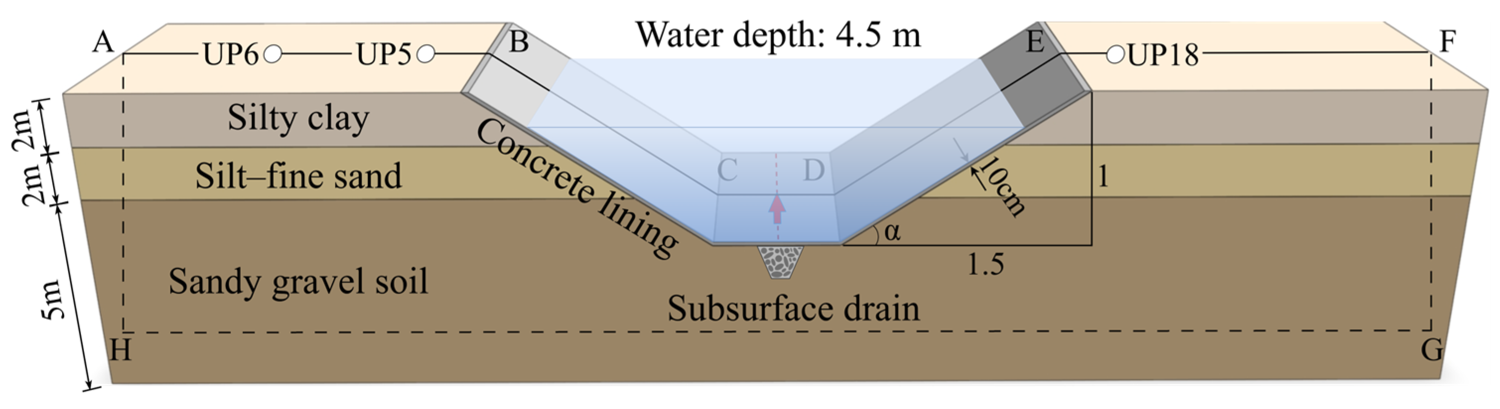
The headrace canal of the HLJ Hydropower Station has a total length of 4.738 km, a design discharge of 98.2 m³/s, and a normal operating water depth of 4.5 m. The canal has a trapezoidal cross-section, with a side slope ratio of 1V:1.5H and a depth of 5.7 m. The lining consists of 100-mm-thick cast-in-place C20 concrete combined with a composite seepage-control system comprising two geotextile layers and one geomembrane. A longitudinal subsurface drain is installed beneath the canal bottom to collect and discharge seepage water from underneath the lining [28].

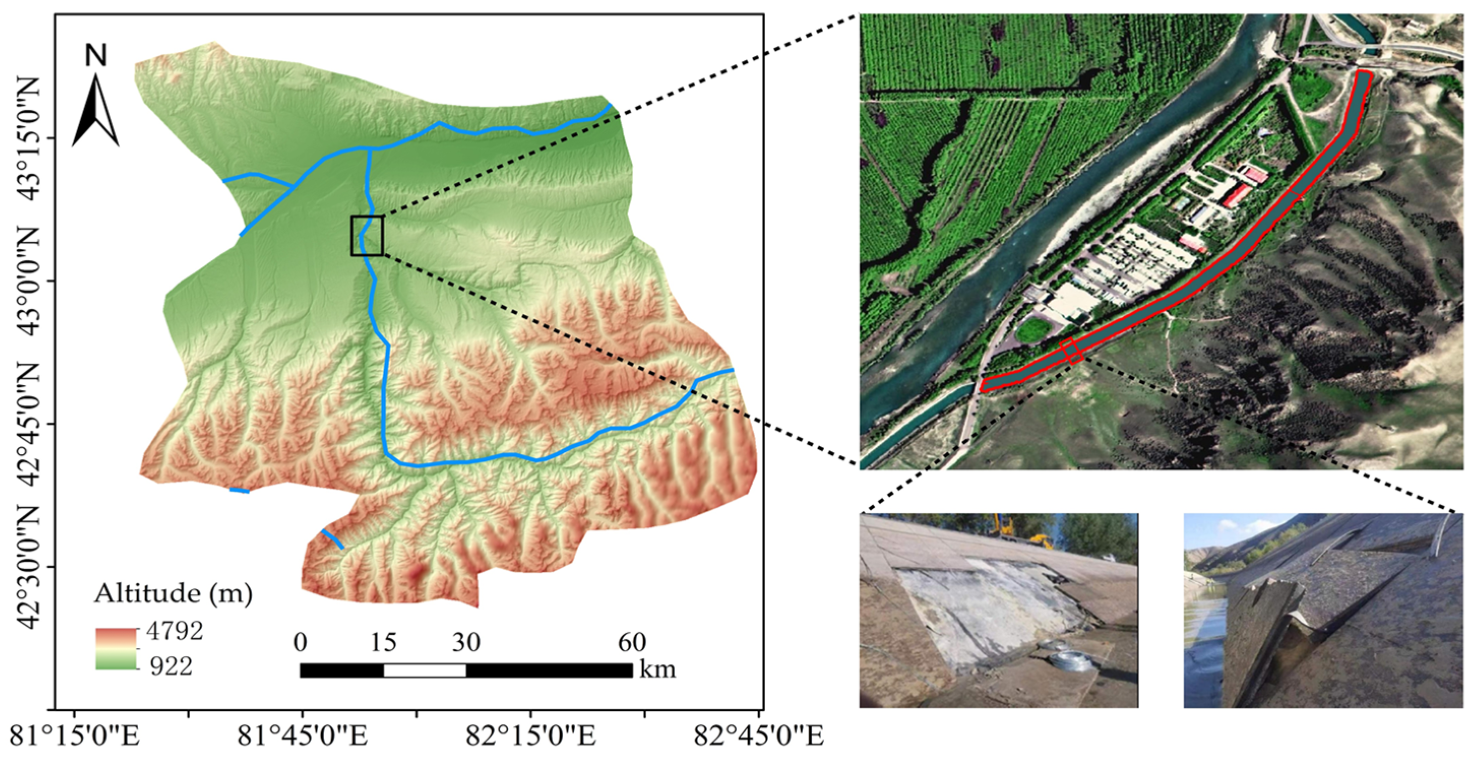
Field investigations indicated that the existing subsurface drainage system had become ineffective because of clogging and other factors. In particular, inadequate drainage along the K0 + 350–K0 + 970 reach resulted in considerable groundwater uplift pressure, causing varying degrees of heaving, cracking, and sliding failure of the canal lining. An overview of the study area and representative lining damage is presented in Figure 1.

This reach is an excavated canal section. From top to bottom, the strata consist of a proluvial silty clay layer, a silt–fine sand layer, and a sand–gravel layer. The sand–gravel layer, with an average thickness of approximately 5 m, serves as the principal aquifer because of its relatively high permeability and is therefore the key stratum controlling groundwater flow. The canal geometry and stratigraphic profile are illustrated in Figure 2.

2.2. Hydrogeological Conditions

2.2.1. Field Monitoring System and Dataset

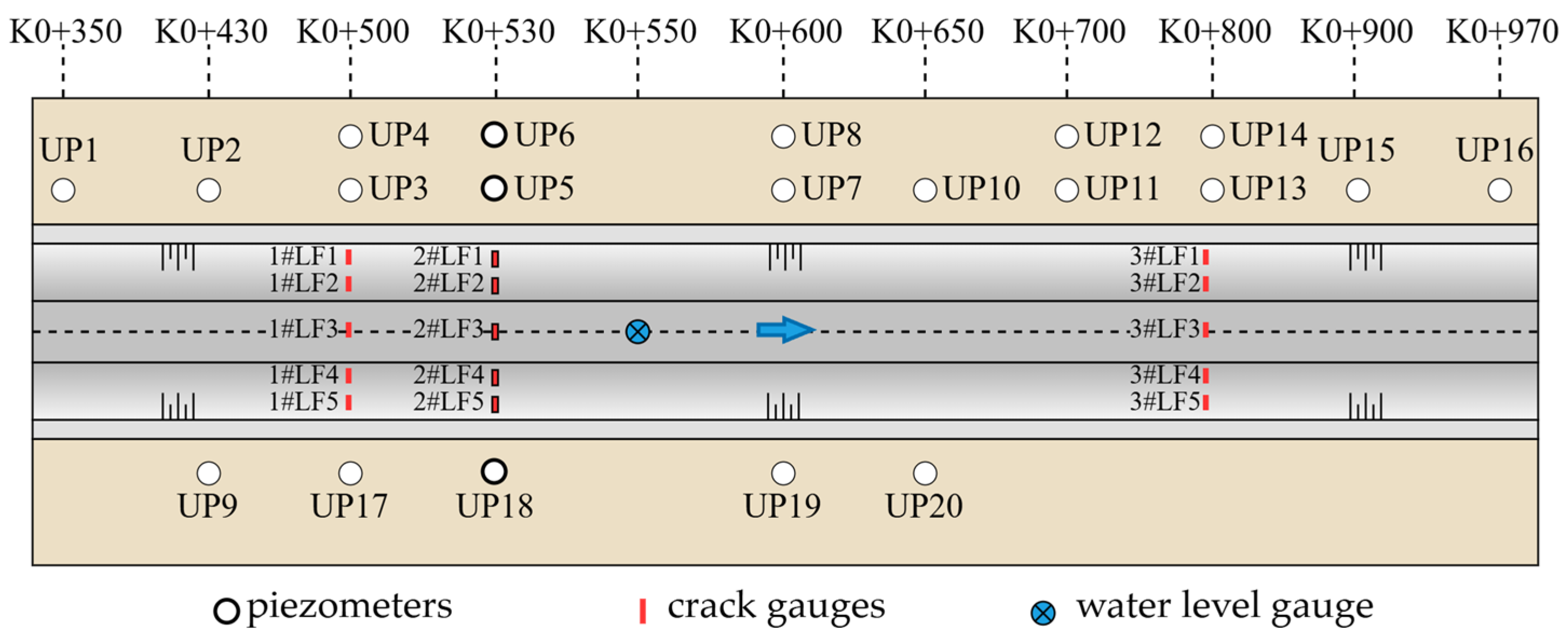
Along both sides of the K0 + 350–K0 + 970 canal reach, 20 piezometers were installed for long-term groundwater monitoring. The monitoring dataset used in this study covers the period from December 2024 to July 2026. In accordance with Design specification for safety monitoring in water and hydropower projects (SL 725-2024) [29], piezometric heads and crack-gauge displacements were automatically recorded at 10 min intervals, whereas the canal water level was recorded at 5 min intervals.

In accordance with Technical specification for earth-rockfill dam safety monitoring (SL 551-2024) [30], three representative monitoring sections, designated Sections 1#, 2#, and 3#, were established along the canal to monitor lining deformation within the damaged reach. Five crack gauges were installed at each section to record the deformation of the canal lining. In addition, a water-level gauge was installed within the monitored reach to continuously record variations in the canal water level. The locations and identification numbers of the piezometers, crack gauges, and canal water-level gauge are shown in Figure 3.

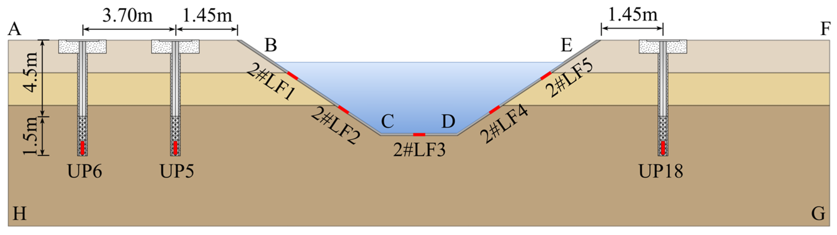
At the representative damaged section at chainage K0 + 530, piezometers UP5, UP6, and UP18 and crack gauges 2#LF1–2#LF5 were selected for detailed analysis. Their cross-sectional arrangement is shown in Figure 4. Piezometers UP5, UP6, and UP18 were approximately 6 m deep, with a screened interval of approximately 1.5 m. The bottom of the screened interval was located approximately 0.3 m below the canal-bottom elevation, with the screened section extending into the sand–gravel layer.

Analysis of the monitoring records showed that groundwater piezometric heads within the investigated reach varied substantially over the monitoring period. The maximum recorded piezometric head reached approximately 3.0 m above the canal bottom and was observed at piezometer UP18 on 8 May 2026. Piezometric heads approximately 3.0 m above the canal bottom persisted for a cumulative duration of approximately 18 days during the monitoring period, indicating that the high-groundwater condition was not merely an isolated observation. Given the magnitude and persistence of the observed high groundwater levels, the maximum recorded groundwater level was adopted as the adverse groundwater condition for the subsequent seepage analysis and relief-well system design.

2.2.2. Hydraulic Conductivity Inputs and Cross-Condition Validation

The hydraulic conductivities of the canal-foundation soils were previously estimated through inverse analysis using a machine-learning-assisted finite-element approach [31]. The inversion algorithm, parameter-search procedure, and convergence assessment are described in detail in Ref. [31] and are therefore not repeated here. In the previous inversion study, a monitoring condition with a relatively stable canal water level and complete piezometric observations was used for parameter calibration. For the present study, a hydraulically distinct monitoring condition that was not used in the parameter inversion was selected for cross-condition validation. The corresponding canal water depths and observed piezometric heads are summarized in

Table 1. Hydraulic conditions and observed relative piezometric heads used for parameter inversion and cross-condition validation.

Condition	Representative Date	Canal Water Depth, hc/m	UP5 h/m	UP6 h/m	UP18 h/m
Calibration (inversion)	1 July 2025	1.4	−1.06	0.21	−1.16
Cross-condition validation	3 April 2026	2.7	−0.17	0.88	−0.23

Note: All piezometric heads are referenced to the canal-bottom elevation at the representative K0 + 530 section. The validation condition was excluded from the parameter inversion.

.

Prior search ranges for hydraulic conductivity were established from the engineering geological investigation. Each soil layer was represented as hydraulically isotropic in the numerical model. The prior search ranges and the corresponding inverted hydraulic conductivities are listed in

Table 2. Prior search ranges and inverted hydraulic conductivities of the canal-foundation soils.

Soil Layer	Average Thickness, d/m	Prior Search Range of K/(m·s−1)	Inverted K/(m·s−1)
Silty clay	2	5.2 × 10−7–1.2 × 10−6	8.10 × 10−7
Silt–fine sand	2	8.4 × 10−6–1.0 × 10−5	8.90 × 10−6
Sand–gravel layer	5	6.0 × 10−5–5.8 × 10−4	4.03 × 10−4

.

To evaluate whether the inverted hydraulic conductivity parameter set could reproduce the groundwater-head field under a hydraulic condition different from that used for inversion, a cross-condition forward simulation was conducted using the validation condition listed in Table 1. The model geometry and hydraulic conductivity parameters were kept unchanged, whereas the external hydraulic-head boundary conditions were updated to represent the validation condition. The observed heads at UP5, UP6, and UP18 were not prescribed as numerical boundary conditions; instead, these piezometers were used solely as internal validation points. The simulated and observed relative piezometric heads are compared in

Table 3. Observed and simulated relative piezometric heads under the cross-condition validation condition.

Piezometer	Observed Head/m	Simulated Head/m	Absolute Error/m
UP5	−0.17	−0.09	0.08
UP6	0.88	0.79	0.09
UP18	−0.23	−0.11	0.12

.

Across the three validation points, the absolute differences between the simulated and observed relative piezometric heads ranged from 0.08 to 0.12 m, with a mean absolute error (MAE) of 0.097 m and a root-mean-square error (RMSE) of 0.098 m. The simulated results reproduced the overall magnitude and spatial variation in the observed piezometric heads under a hydraulic condition that was excluded from the parameter inversion. These results provide independent cross-condition validation of the transferability of the inverted parameter set for the subsequent relief-well simulations.

2.3. Anti-Uplift Stability Criterion for the Canal Lining

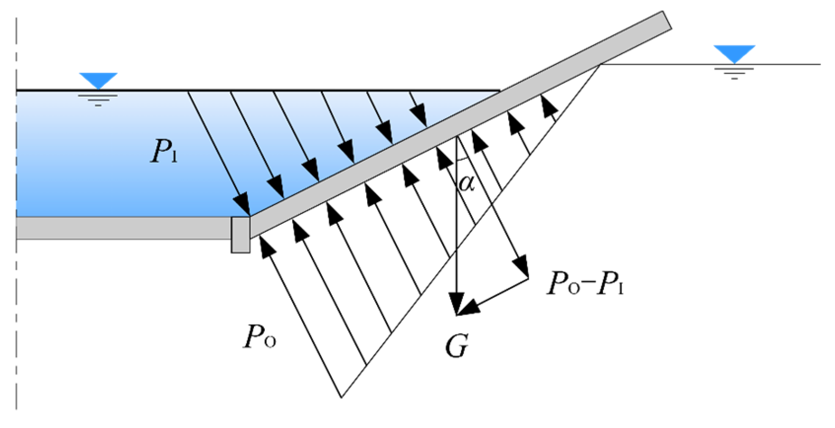
The anti-uplift stability of the canal lining was evaluated in accordance with the Design Specifications for Sluices (SL 265-2016) [32]. Under the design verification condition, the anti-uplift safety factor of the lining should not be less than 1.05. Therefore, K_f = 1.05 was adopted as the control criterion in this study. As illustrated in Figure 5, the lining is primarily subjected to three forces under groundwater loading: the water pressure exerted by the canal water on the lining, P_I; the groundwater uplift force acting beneath the lining, P_O; and the self-weight of the lining, G.

For a given lining thickness, the anti-uplift stability criterion for the canal bottom lining can be expressed as

$$K_f={\displaystyle \frac{G}{P_O-P_I}}$$

(1)

where K_f is the anti-uplift safety factor of the canal lining; G is the self-weight of the lining slab, kN; P_I is the water pressure exerted by the canal water on the lining slab, kN; and P_O is the groundwater uplift force acting on the lining slab, kN.

The empty-canal condition during maintenance was considered the most unfavorable condition for the anti-uplift stability assessment. Under this condition, the water pressure acting on the upper surface of the lining slab was taken as zero. The calculation was performed using a saturated unit weight of 24 kN/m³ for the C20 concrete and a lining thickness of 0.1 m. When the anti-uplift safety factor of the canal bottom lining satisfies K_f ≥ 1.05, the maximum allowable relative uplift pressure head is 0.23 m.

Taking the canal-bottom elevation as the reference datum, the relative uplift pressure head at the canal bottom is defined as

$$H=h_p-z_b$$

(2)

where h_p is the piezometric head elevation at the control point of the canal bottom, m, and z_b is the elevation of the canal bottom slab, m. When H > 0, the piezometric level is above the canal bottom slab; when H < 0, the piezometric level is below the canal bottom slab.

2.4. Finite-Element Model and Boundary Conditions

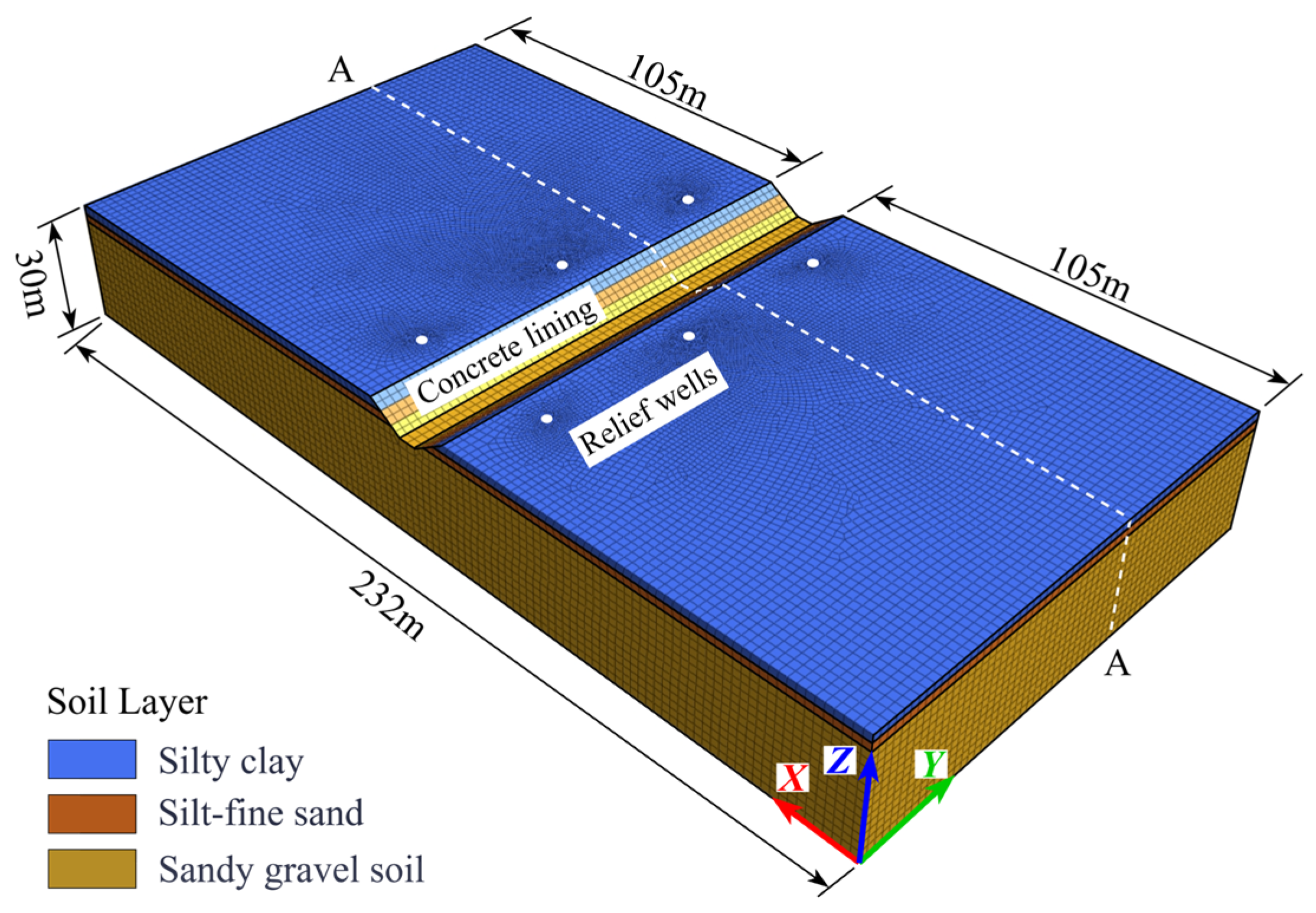
A three-dimensional numerical seepage model of the headrace canal at the HLJ Hydropower Station was established based on the engineering geological investigation data and hydrogeological characteristics of the study area. The section at chainage K0 + 530 was selected as the reference section of the computational domain. In the Y-direction, the model covered the dewatering influence zone of three adjacent groups of relief wells. In the X-direction, the lateral boundaries were placed sufficiently far from the canal and relief wells to reduce the influence of the prescribed far-field boundary conditions on the seepage response within the primary analysis region. Specifically, the computational domain extended approximately 105 m [33]. In the Z-direction, the domain extended 30 m downward into the foundation. The A–A section located midway between adjacent relief wells was selected as the primary analysis section. Particular attention was given to the distribution of the relative uplift pressure head beneath the canal bottom to determine whether the anti-uplift stability requirement of the lining was satisfied.

Figure 6 presents the computational mesh and the locally refined mesh around the relief wells for Run 5. The meshes used for the other runs differed slightly according to the corresponding well configurations. As shown in Figure 6, the mesh size was gradually refined from approximately 1 m in the far-field region to approximately 0.1 m near the wells to improve the accuracy of the local seepage-field simulation. The resulting finite-element model comprised approximately 1,319,220 nodes and 1,945,940 elements, enabling an adequate representation of the seepage characteristics within the study area.

The numerical model represented three-dimensional steady-state seepage through a heterogeneous but isotropic porous medium. To ensure the accuracy of the seepage analysis, the relief wells were explicitly modeled according to the actual engineering configuration. The canal-bottom lining surface, side-slope lining surfaces, upstream and downstream truncation planes, and the bottom surface of the computational domain were assigned no-flow boundary conditions. The far-field boundaries on both sides of the canal were prescribed as constant-head boundaries to represent the regional groundwater-head condition [13,34]. Each relief well was simulated using a combination of constant-head and seepage-face boundary conditions. The well wall below the prescribed pumping control water level was assigned a constant-head boundary, whereas the well wall above this level was assigned a seepage-face boundary [35].

2.5. Experimental Design and Optimization Method

2.5.1. Response Surface Experimental Design for the Dewatering System

Based on the engineering conditions and hydrogeological characteristics of the study area, the horizontal distance from the relief wells to the canal edge, x₁, the relief-well spacing, x₂, and the depth to the pumping control water level, x₃, were selected as the principal design variables. The relative uplift pressure head at the canal bottom, H, and the single-well pumping rate, q, were taken as the response variables. Because well diameter has a relatively limited effect on dewatering performance and is constrained by the applicable code requirements, it was fixed at 0.4 m and was not included as a response surface design variable. The ranges of x₁, x₂, and x₃ were determined in accordance with the Technical Code for Tube Well (GB 50296-2014) [36] and the site construction conditions.

(1)

Horizontal distance from the relief wells to the canal edge

Considering the site topography and construction feasibility, the relief wells were arranged within the canal berm. Taking into account the required setback from the canal edge and the space needed for construction, operation, and maintenance, the experimental levels of x₁ were set at 1, 8, and 15 m.

(2)

Relief-well spacing

The relief-well spacing was determined with reference to the influence radius of an individual relief well, which can be estimated as follows:

$$R=3000S\sqrt{K}$$

(3)

where R is the influence radius of a relief well, m; S is the drawdown of the confined groundwater head, m; and K is the equivalent hydraulic conductivity of the aquifer system, m/s.

Owing to the pronounced stratification of the subsurface strata in the study area and the substantial differences in hydraulic conductivity among individual layers, the use of a single-layer hydraulic conductivity cannot adequately characterize the overall groundwater flow behavior of the multilayer aquifer system. Therefore, based on the thicknesses and hydraulic conductivities of the saturated layers below the initial groundwater level, the equivalent hydraulic conductivity was calculated using the thickness-weighted average [37]:

$$K_{eq}={\displaystyle \frac{{\displaystyle \sum _{i=1}^n{K}_i}{h}_i}{H}}$$

where K_i and h_i are the hydraulic conductivity, m/s, and thickness, m, of the i-th saturated layer, respectively; and H is the total saturated thickness involved in groundwater flow, m.

The initial groundwater level at the study site was located within the silt–fine sand layer at approximately 2.70 m below the ground surface. The bottom of the silt–fine sand layer was located at 4.00 m below the ground surface; thus, its initial saturated thickness was 1.30 m, with a hydraulic conductivity of 8.9 × 10⁻⁶ m/s. The underlying sand–gravel layer had a thickness of 5.00 m and a hydraulic conductivity of 4.03 × 10⁻⁴ m/s. Accordingly, the total saturated thickness under the initial condition was 6.30 m, and the equivalent hydraulic conductivity was calculated as 3.22 × 10⁻⁴ m/s. Substitution into Equation (3) yielded an estimated influence radius of approximately 150 m. Based on this estimate and subsequent preliminary calculations, the spacing range was further refined, and 10, 40, and 70 m were selected as the experimental levels of x₂.

(3)

Depth to the pumping control water level

The depth to the pumping control water level is defined as the vertical distance from the wellhead to the prescribed water level inside the relief well. This depth must satisfy the well-depth constraint. According to the relevant code, the required relief-well depth can be estimated as follows:

$$H_w=H_{w1}+H_{w2}+H_{w3}$$

(4)

where H_w is the total depth of the relief well, m; H_w1 is the burial depth of the top of the target aquifer, m; H_w2 is the distance from the bottom of the well screen to the top of the target aquifer, m; and H_w3 is the length of the sump section, m.

The well-screen length was set to 5 m, corresponding to the thickness of the target aquifer; the sump length was set to 2 m; and the burial depth of the target aquifer was 4 m. The resulting design depth of the relief well was approximately 11 m. The pumping control water level must remain above the well bottom (x₃ < H_w), and sufficient clearance must be reserved for the sump and safe pump operation. Accordingly, 6, 8, and 10 m were selected as the experimental levels of x₃.

In summary, a Box–Behnken experimental design [38] was employed to establish quadratic response surface models relating the three design variables x₁, x₂, and x₃ to the relative uplift pressure head at the canal bottom, H, and the single-well pumping rate, q. The factor levels and coded values are presented in

Table 4. Factor levels and coded values.

Coded Level	x1/m	x2/m	x3/m
−1	1	10	6
0	8	40	8
1	15	70	10

.

2.5.2. Multi-Objective Optimization Model Based on NSGA-II

To reduce the construction scale of the relief-well system and the operational pumping demand while ensuring the anti-uplift stability of the canal lining, a multi-objective optimization model was developed. The Pareto-optimal solutions were generated using NSGA-II, an elitist evolutionary algorithm based on nondominated sorting and crowding-distance preservation [39]. The objective functions included the deviation of the relative uplift pressure head at the canal bottom from its allowable threshold, the number of relief wells within the study reach, and the total pumping rate.

The first objective was to minimize the deviation of the relative uplift pressure head from the allowable threshold. Subject to the anti-uplift stability requirement, the relative uplift pressure head was constrained to remain as close as possible to the allowable threshold to avoid excessive groundwater drawdown:

$$\begin{array}{l}\min F_1(x)=H^{*}-H(x)\\ s.t. H^{*}\ge H(x)\end{array}$$

(5)

where H(x) is the predicted relative uplift pressure head at the canal bottom, m; H* is the maximum allowable relative uplift pressure head for anti-uplift stability and was set to 0.23 m; and x = (x₁, x₂, x₃) denotes the vector of design variables.

The second objective was to minimize the total number of relief wells:

$$\min F_2(x)=N(x_2)=2⌈{\displaystyle \frac{L}{x_2}}⌉$$

(6)

where N(x₂) is the total number of relief wells installed along both sides of the canal; L is the length of the study reach, m; x₂ is the relief-well spacing, m; and ⌈L/x₂⌉ denotes the smallest integer greater than or equal to L/x₂, representing the number of relief wells along one side of the canal.

The third objective was to minimize the total pumping rate:

$$\min F_3(x)=Q (x)=N(x_2)q(x)$$

(7)

where Q(x) is the total pumping rate within the study reach, m³/s, and q(x) is the predicted pumping rate of a single relief well, m³/s.

Accordingly, the multi-objective optimization model can be expressed as

$$\begin{array}{l}\min F(x)=\left[F_1(x), F_2(x), F_3(x)\right]\\ s.t. \left\{\begin{array}{l}{H}^{*}\ge H(x)\\ x_i^{-}\le x_i\le x_i^{+}, i=1, 2, 3\end{array}\right.\end{array}$$

(8)

2.5.3. Hydraulic Conductivity Sensitivity Analysis and Sensitivity-Based Screening Method

Although the hydraulic conductivity parameters adopted in the finite-element model were obtained through the inverse analysis described above and further evaluated through the cross-condition validation presented in Section 2.2.2, natural foundation soils exhibit pronounced spatial heterogeneity. In addition, uncertainties inevitably arise from seepage tests and parameter inversion. Therefore, the hydraulic conductivity parameters remain subject to a certain degree of uncertainty. To evaluate the influence of hydraulic conductivity uncertainty on the hydraulic response of the relief well design and to avoid selecting solutions that are too close to the safety control limit based solely on deterministic parameter conditions, a hydraulic conductivity sensitivity analysis was conducted for the Pareto-optimal solution set. A hydraulic-conductivity sensitivity margin was then established based on the maximum adverse increase in uplift pressure head induced by parameter perturbations and was used to pre-screen the Pareto candidate solutions.

First, a representative solution P_M with intermediate trade-off characteristics was selected from the Pareto-optimal solution set and used as the baseline solution for the subsequent hydraulic conductivity sensitivity analysis. The representative solution was selected from the M Pareto-optimal solutions obtained from the preceding multi-objective optimization. Because the objective functions differ in scale and magnitude, min–max normalization was first applied to the three objective functions to eliminate the influence of scale differences on the distance calculation. For the j-th objective of the i-th Pareto solution, the normalized value is defined as:

$$z_{ij}={\displaystyle \frac{f_{ij}-f_{j,\min }}{f_{j,\max }-f_{j,\min }}},\hspace{1em}i=1,2,\dots , M;\hspace{1em}j=1,2,3$$

(9)

where f_ij is the value of the j-th objective function for the i-th Pareto solution; f_j,min and f_j,max are the minimum and maximum values, respectively, of the j-th objective function among all Pareto-optimal solutions; z_ij is the normalized objective-function value; and M is the total number of Pareto-optimal solutions.

In the normalized objective space, the geometric center of all Pareto-optimal solutions is adopted as a reference point representing the intermediate trade-off region of the solution set. The coordinate of the geometric center along the j-th objective dimension is calculated as:

$$c_j={\displaystyle \frac{1}{M}}{\displaystyle \sum _{i=1}^M{z}_{ij}},\hspace{1em}j=1,2,3$$

(10)

Accordingly, the geometric center in the three-dimensional normalized objective space is expressed as:

$$C=\left(c_1, c_2, c_3\right)$$

(11)

The Euclidean distance was then used to quantify the proximity of each Pareto-optimal solution to the geometric center. The distance between the i-th Pareto solution and the geometric center is calculated as:

$$D_i=\sqrt{{(z_{i1}-c_1)}^2+{(z_{i2}-c_2)}^2+{(z_{i3}-c_3)}^2}$$

(12)

A smaller Euclidean distance indicates that the solution is closer to the intermediate region of the Pareto set in the normalized objective space and therefore exhibits a relatively balanced trade-off among the objectives. Accordingly, the Pareto-optimal solution with the minimum distance to the geometric center was selected as the representative solution for the hydraulic conductivity sensitivity analysis. Its index i* and the corresponding representative solution P_M are defined as:

$$i^{*}=\underset{ i=1,2,\dots ,M}{\arg \underset{i}{\min }{D}_i},\hspace{1em}{P}_M=P_{i^{*}}$$

(13)

After the representative solution P_M was determined, a one-factor-at-a-time sensitivity analysis of the hydraulic conductivity parameters was conducted using this solution as the baseline. During the analysis, the design variables, model geometry, boundary conditions, and relief well control scheme of P_M were kept unchanged, while the hydraulic conductivity of each soil layer was varied individually to isolate its influence on the hydraulic response at the canal bottom. The baseline values and perturbation ranges of the hydraulic conductivity parameters were specified according to the parameter ranges determined in Table 2. Following the principle that only one soil-layer hydraulic conductivity was varied at a time while those of the remaining layers were kept at their baseline values, one baseline scenario (S₀) and six single-factor perturbation scenarios (S₁–S₆) were established, as shown in

Table 5. Scenarios for hydraulic conductivity sensitivity analysis.

Scenario	Silty Clay K1/(m·s−1)	Silt–Fine Sand K2/(m·s−1)	Sand–Gravel Layer K3/(m·s−1)
S0	8.10 × 10−7	8.90 × 10−6	4.03 × 10−4
S1	5.20 × 10−7	8.90 × 10−6	4.03 × 10−4
S2	1.20 × 10−6	8.90 × 10−6	4.03 × 10−4
S3	8.10 × 10−7	8.40 × 10−6	4.03 × 10−4
S4	8.10 × 10−7	1.00 × 10−5	4.03 × 10−4
S5	8.10 × 10−7	8.90 × 10−6	6.00 × 10−5
S6	8.10 × 10−7	8.90 × 10−6	5.80 × 10−4

.

Finite-element seepage analyses were performed for each scenario, and the relative uplift pressure head at the canal bottom was extracted. Taking the relative uplift pressure head H₀ under the baseline scenario S₀ as the reference, the change in uplift pressure head induced by the i-th perturbation scenario is defined as:

$$\mathsf{\Delta }{H}_i=H_i-H_0,\hspace{1em}i=1,2,\dots ,6$$

(14)

where H_i is the relative uplift pressure head at the canal bottom under the i-th perturbation scenario. When ΔH_i > 0, the hydraulic conductivity perturbation increases the relative uplift pressure head at the canal bottom and is therefore unfavorable to hydraulic safety; when ΔH_i < 0, the relative uplift pressure head decreases.

Because the adverse effect of hydraulic conductivity variations on engineering safety is primarily reflected by an increase in the relative uplift pressure head at the canal bottom, the maximum positive head increment among all perturbation scenarios was taken as the hydraulic-conductivity sensitivity margin associated with hydraulic conductivity uncertainty and denoted by ΔH_max. Accordingly, the sensitivity-adjusted screening threshold is defined as

$$H_s=0.23-\mathsf{\Delta }{H}_{\max }$$

(15)

Subsequently, H_s was used as the sensitivity-adjusted screening threshold for the Pareto candidate solutions. Solutions with a relative uplift pressure head at the canal bottom not exceeding this threshold were retained and subsequently evaluated using the entropy-weighted TOPSIS method.

2.5.4. Comprehensive Decision-Making Using the Entropy-Weighted TOPSIS Method

To select a final design from the Pareto-optimal candidate solutions generated by NSGA-II, the entropy-weighted Technique for Order Preference by Similarity to Ideal Solution (TOPSIS) method, originally developed within the multiple-attribute decision-making framework by Hwang and Yoon [40], was employed for post-optimization decision-making. The entropy-weighting method determines objective weights according to the degree of variation in each evaluation indicator, whereas TOPSIS ranks the candidate solutions by comparing their distances from the positive and negative ideal solutions. A larger relative closeness value indicates that a candidate solution is closer to the overall ideal solution.

(1)

Construction of the original evaluation matrix

The m candidate dewatering schemes on the Pareto front were taken as the alternatives to be evaluated, and their corresponding n evaluation indicators were used to construct the original evaluation matrix:

$$A={\left(a_{ij}\right)}_{m\times n}\left(\begin{array}{cccc}{a}_{11}& a_{12}& \dots & a_{1n}\\ a_{21}& a_{22}& \dots & a_{2n}\\ ⋮& ⋮& \ddots & ⋮\\ a_{m1}& a_{m2}& \dots & a_{mn}\end{array}\right)$$

(16)

where A is the original evaluation matrix; a_ij is the original value of the j-th indicator for the i-th candidate solution; i = 1, 2, …, m; j = 1, 2, …, n; m is the number of candidate solutions; and n is the number of evaluation indicators.

(2)

Construction of the normalized decision matrix

The evaluation indicators considered in this study were the deviation of the relative uplift pressure head at the canal bottom, F₁, the number of relief wells within the study reach, F₂, and the total pumping rate, F₃. All three indicators are cost-type criteria, for which a smaller value represents better performance. To eliminate the effects of differences in dimensions and numerical scales, the original evaluation matrix was transformed and normalized as follows:

$$b_{ij}={\displaystyle \frac{max(a_{ij})-a_{ij}}{max(a_{ij})-min(a_{ij})}}$$

(17)

where b_ij is the dimensionless benefit-type value of the jth indicator for the ith candidate solution. A larger b_ij value indicates better performance.

(3)

Determination of entropy weights

Based on the normalized decision matrix, the information entropy of each indicator was calculated, and the corresponding objective weights were then determined as follows:

$$w_j={\displaystyle \frac{1-e_j}{{\displaystyle \sum _{j=1}^n(1-e_j)}}}$$

(18)

where w_j denotes the entropy weight of the jth evaluation indicator, and e_j represents the information entropy of the jth evaluation indicator.

(4)

Construction of the weighted decision matrix

$$c_{ij}=w_j\times b_{ij}$$

(19)

where c_ij denotes the element in the ith row and jth column of the weighted decision matrix.

(5)

Determination of the positive and negative ideal solutions

$$\left\{\begin{array}{l}{C}^{+}=\left\{c_1^{+}, c_2^{+}, \dots , c_n^{+}\right\}\\ C^{-}=\left\{c_1^{-}, c_2^{-}, \dots , c_n^{-}\right\}\end{array}\right.$$

(20)

where C⁺ and C⁻ denote the positive and negative ideal solution sets, respectively; $c_j^{+}$ and $c_j^{-}$ denote the corresponding positive and negative ideal values of the jth evaluation indicator.

(6)

Calculation of the distances to the positive and negative ideal solutions

After the normalized decision matrix was weighted, the positive and negative ideal solutions were constructed. The Euclidean distances from each candidate solution to the positive and negative ideal solutions were calculated as follows:

$$\left\{\begin{array}{l}{D}_i^{+}=\sqrt{{\displaystyle \sum _{j=1}^n{(c_{ij}-c_j^{+})}^2}}\\ D_i^{-}=\sqrt{{\displaystyle \sum _{j=1}^n{(c_{ij}-c_j^{-})}^2}}\end{array}\right.$$

(21)

where $D_i^{+}$ and $D_i^{-}$ denote the distances of the ith alternative from the positive and negative ideal solutions, respectively.

(7)

Calculation of the relative closeness to the ideal solution

The relative closeness of each candidate solution to the ideal solution was calculated as

$$O_i={\displaystyle \frac{D_i^{-}}{D_i^{+}+D_i^{-}}}$$

(22)

where O_i denotes the relative closeness coefficient of the ith alternative. The closer O_i is to 1, the closer the alternative is to the overall ideal state.

2.5.5. TOPSIS Weight Sensitivity Analysis

To evaluate the robustness of the TOPSIS ranking to variations in the criterion weights, a Monte Carlo-based weight sensitivity analysis was performed. The entropy weights obtained in Section 2.5.4 were used as the baseline weights. For each simulation, the weight of each criterion was independently perturbed within a prescribed range and subsequently renormalized as

$$w_j^{\prime }={\displaystyle \frac{w_j\left(1+{\epsilon }_j\right)}{{\displaystyle \sum _{k=1}^3{w}_k}\left(1+{\epsilon }_k\right)}},\hspace{1em}{\epsilon }_j~U(-\alpha ,\alpha )$$

(23)

where w_j and $w_j^{\prime }$ denote the original and perturbed weights, respectively, and $\mathsf{\alpha }$ represents the perturbation amplitude. Two perturbation levels, $\mathsf{\alpha } = 0$.10 and 0.20, corresponding to ±10% and ±20% variations in the original weights, were considered.

For each perturbation level, 10,000 Monte Carlo simulations were conducted. In each simulation, the TOPSIS ranking was recalculated using the perturbed weights. The stability of the decision result was evaluated using the probability that the original optimal solution remained ranked first (Top-1 rate), the probability that it remained within the top three (Top-3 rate), its mean rank, and the mean Spearman rank correlation coefficient between the perturbed and original rankings. Higher Top-1 and Top-3 rates, a mean rank closer to 1, and a Spearman coefficient closer to 1 indicate greater ranking robustness.

2.6. Analysis Workflow

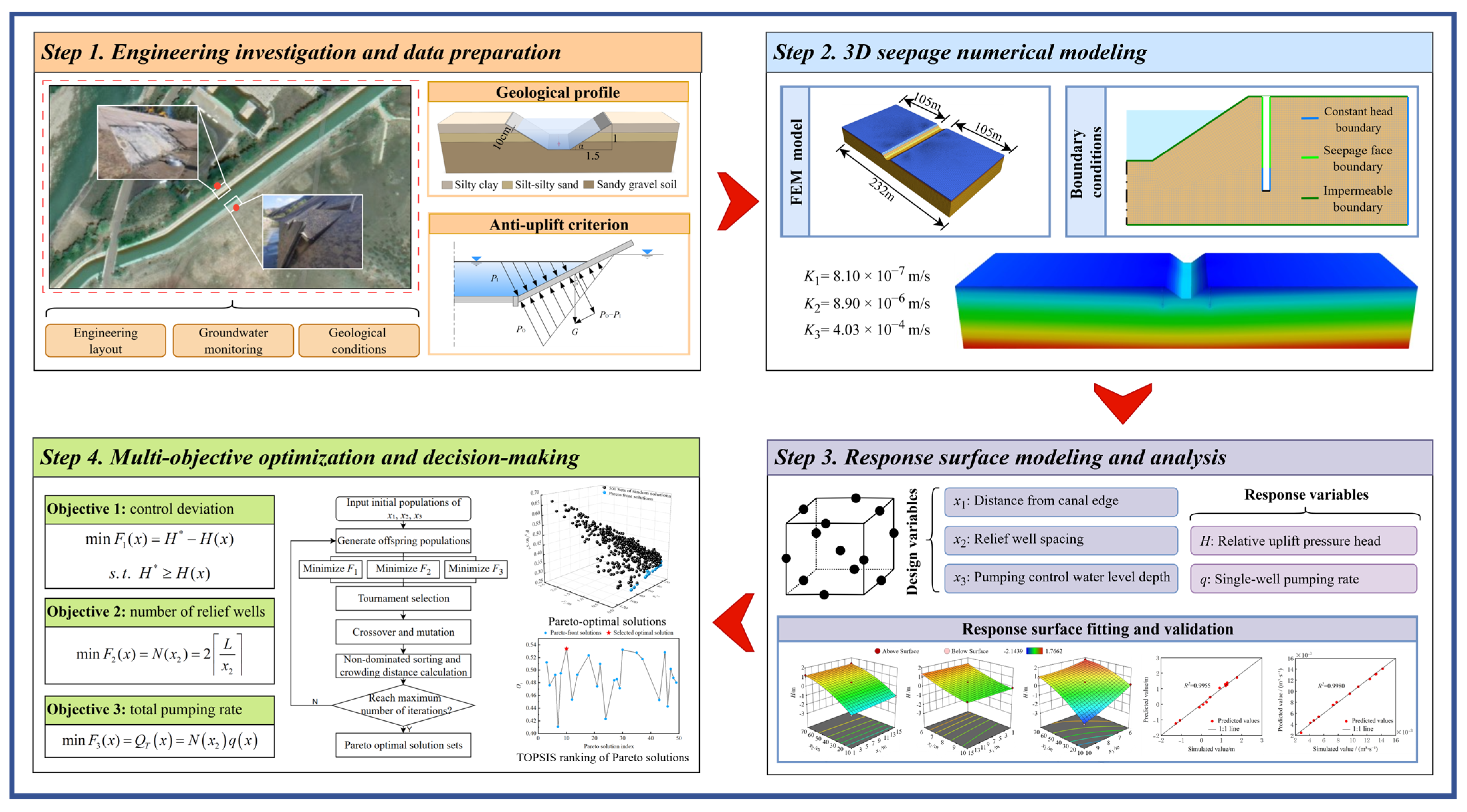
The proposed analysis and optimization framework mainly comprised the following steps: hydrogeological characterization and cross-condition validation of the finite-element model; determination of the design variables; Box–Behnken experimental design; steady-state finite-element seepage simulations; development of the response surface models; NSGA-II-based multi-objective optimization; generation of the M Pareto-optimal solutions; hydraulic conductivity sensitivity analysis and sensitivity-based screening; comprehensive decision-making using the entropy-weighted TOPSIS method; TOPSIS weight sensitivity analysis; and finite-element verification of the selected design.

Within this framework, the anti-uplift stability requirement of the canal lining was treated as the primary hydraulic constraint, while the number of relief wells and the total pumping rate were used to characterize the construction scale and dewatering demand, respectively. The procedure therefore aimed to identify a relief-well configuration that provides adequate hydraulic safety while avoiding unnecessarily large system scale and pumping demand. The overall analysis and optimization workflow is illustrated in Figure 7.

3. Results

3.1. Results of the Box–Behnken Design

A Box–Behnken design was employed to generate combinations of the design variables for the relief-well dewatering system. The horizontal distance from the relief wells to the canal edge, x₁, the relief-well spacing, x₂, and the depth to the pumping control water level, x₃, were selected as the independent variables, resulting in a total of 17 design runs.

For each design run, numerical simulations were performed using the established finite-element seepage model. After numerical convergence was achieved, the relative uplift pressure head at the center of the canal bottom along the A–A control section, located midway between two adjacent groups of relief wells, and the single-well pumping rate were extracted as the response variables. The calculated responses were subsequently used to develop the response surface models through regression analysis. The design matrix and corresponding simulation results are presented in

Table 6. Box–Behnken design matrix and response results.

Run	x1/m	x2/m	x3/m	H/m	q/(m3·s−1)
1	1	40	6	1.1962	0.0073
2	15	40	6	1.2929	0.0078
3	1	70	8	1.2167	0.0132
4	15	40	10	0.0763	0.0133
5	8	40	8	0.4431	0.0108
6	8	10	6	0.2595	0.0028
7	1	40	10	−0.1088	0.0124
8	8	40	8	0.4431	0.0108
9	8	40	8	0.4431	0.0108
10	8	70	10	0.9179	0.0161
11	15	70	8	1.2881	0.0142
12	1	10	8	−1.2741	0.0041
13	8	40	8	0.4431	0.0108
14	8	70	6	1.7662	0.0096
15	8	10	10	−2.1439	0.0053
16	8	40	8	0.4431	0.0108
17	15	10	8	−1.0648	0.0046

Note: Negative values of the relative uplift pressure head indicate that the piezometric level is below the canal-bottom elevation.

.

3.2. Development and Validation of the Response Surface Models

3.2.1. Model Development

Based on the data obtained from the Box–Behnken design, least-squares regression analysis was performed to quantify the relationships between the design variables and response variables, thereby establishing quadratic response surface models. The horizontal distance from the relief wells to the canal edge, x₁, the relief-well spacing, x₂, and the depth to the pumping control water level, x₃, were taken as the independent variables, whereas the relative uplift pressure head at the canal bottom, H, and the single-well pumping rate, q, were taken as the response variables. The resulting quadratic polynomial regression models in terms of the actual variables are expressed as follows:

$$\begin{gathered} h=5.72168+0.001926x_1+0.024954x_2-1.29164x_3-0.000164x_1{x}_2+0.001579x_1{x}_3 \\ +0.006480x_2{x}_3+0.000129x_1^2-0.000453x_2^2+0.041187x_3^2 \end{gathered}$$

(24)

$$\begin{gathered} q=-0.012033-0.000025x_1+0.000170x_2+0.002851x_3+5.95238\times {10}^{-7}{x}_1{x}_2 \\ +7.14286\times {10}^{-6}{x}_1{x}_3+1.7\times {10}^{-5}{x}_2{x}_3-2.55102\times {10}^{-7}{x}_1^2-1.95833\times {10}^{-6}{x}_2^2-1.47\times {10}^{-4}{x}_3^2 \end{gathered}$$

(25)

where H is the relative uplift pressure head at the canal bottom, m; q is the single-well pumping rate, m³/s; x₁ is the horizontal distance from the relief well to the canal edge, m; x₂ is the relief-well spacing, m; and x₃ is the depth to the pumping control water level, m.

3.2.2. Model Validation

To evaluate the adequacy of the response surface regression models, analysis of variance (ANOVA) was performed separately for the relative uplift pressure head at the canal bottom, H, and the single-well pumping rate, q. The statistical significance of each model was assessed using the F-test as

$$F={\displaystyle \frac{M_r}{M_e}}={\displaystyle \frac{S_r/\nu }{S_e/(n-\nu -1)}}$$

(26)

where M_r is the regression mean square; M_e is the residual mean square; S_r is the regression sum of squares; S_e is the residual sum of squares; n is the number of experimental runs; and ν is the number of degrees of freedom associated with the regression model.

The F-statistic represents the ratio of the regression mean square to the residual mean square. When the calculated F-value exceeds the corresponding critical value, the regression model is considered statistically significant. The p-value was also used to assess the statistical significance of each regression term. A term was considered highly significant when p < 0.01, significant when 0.01 ≤ p ≤ 0.05, and nonsignificant when p > 0.05.

The ANOVA results for the two response models are presented in

Table 7. Analysis of variance for the quadratic response surface model of H.

Source	Sum of Squares	df	Mean Square	F-Value	p-Value
Model	16.68	9	1.85	170.47	<0.0001
x1	0.0187	1	0.0187	1.72	0.2307
x2	5.14	1	5.14	473.23	<0.0001
x3	2.17	1	2.17	199.38	<0.0001
x1x2	0.0048	1	0.0048	0.4373	0.5296
x1x3	0.002	1	0.002	0.1797	0.6843
x2x3	0.6046	1	0.6046	55.61	0.0001
$x_1^2$	0.0002	1	0.0002	0.0154	0.9048
$x_2^2$	0.7006	1	0.7006	64.45	<0.0001
$x_3^2$	0.1143	1	0.1143	10.51	0.0142
Residual	0.0761	7	0.0109
Pure error	0	4	0
Cor Total	16.75	16

Note: R² = 0.9955; $R_{\mathit{Adj}}^2=0.9896$; $R_{\mathit{Pre}}^2=0.9273.$

and

Table 8. Analysis of variance for the quadratic response surface model of q.

Source	Sum of Squares	df	Mean Square	F-Value	p-Value
Model	0.0002	9	2.59 × 10−5	383.55	<0.0001
x1	5.21 × 10−7	1	5.21 × 10−7	7.72	0.0274
x2	0.0001	1	0.0001	1288.01	<0.0001
x3	2.55 × 10−5	1	2.55 × 10−5	377.07	<0.0001
x1x2	6.25 × 10−8	1	6.25 × 10−8	0.9259	0.368
x1x3	4.00 × 10−8	1	4.00 × 10−8	0.5926	0.4666
x2x3	4.00 × 10−6	1	4.00 × 10−6	59.26	0.0001
$x_1^2$	6.58 × 10−10	1	6.58 × 10−10	0.0097	0.9241
$x_2^2$	1.31 × 10−5	1	1.31 × 10−5	193.77	<0.0001
$x_3^2$	1.45 × 10−6	1	1.45 × 10−6	21.53	0.0024
Residual	4.73 × 10−7	7	6.75 × 10−8
Pure error	0	4	0
Cor Total	0.0002	16

Note: R² = 0.9980; $R_{\mathit{Adj}}^2=0.9954$; $R_{\mathit{Pre}}^2=0.9676.$

. The F-values of the models for the relative uplift pressure head at the canal bottom and the single-well pumping rate were 170.47 and 383.55, respectively. Both models were highly significant overall (p < 0.0001), confirming the statistical significance of the fitted quadratic response surface models. Among the model terms, the relief-well spacing x₂, the depth to the pumping control water level x₃, and the quadratic term ${\mathrm{x}}_2^2$ had highly significant effects on both response variables. These results indicate that the relief-well spacing and depth to the pumping control water level are the principal design variables governing both the uplift-pressure response and the single-well pumping rate. In addition, the highly significant quadratic effect of x₂ indicates a pronounced nonlinear relationship between relief-well spacing and both response variables.

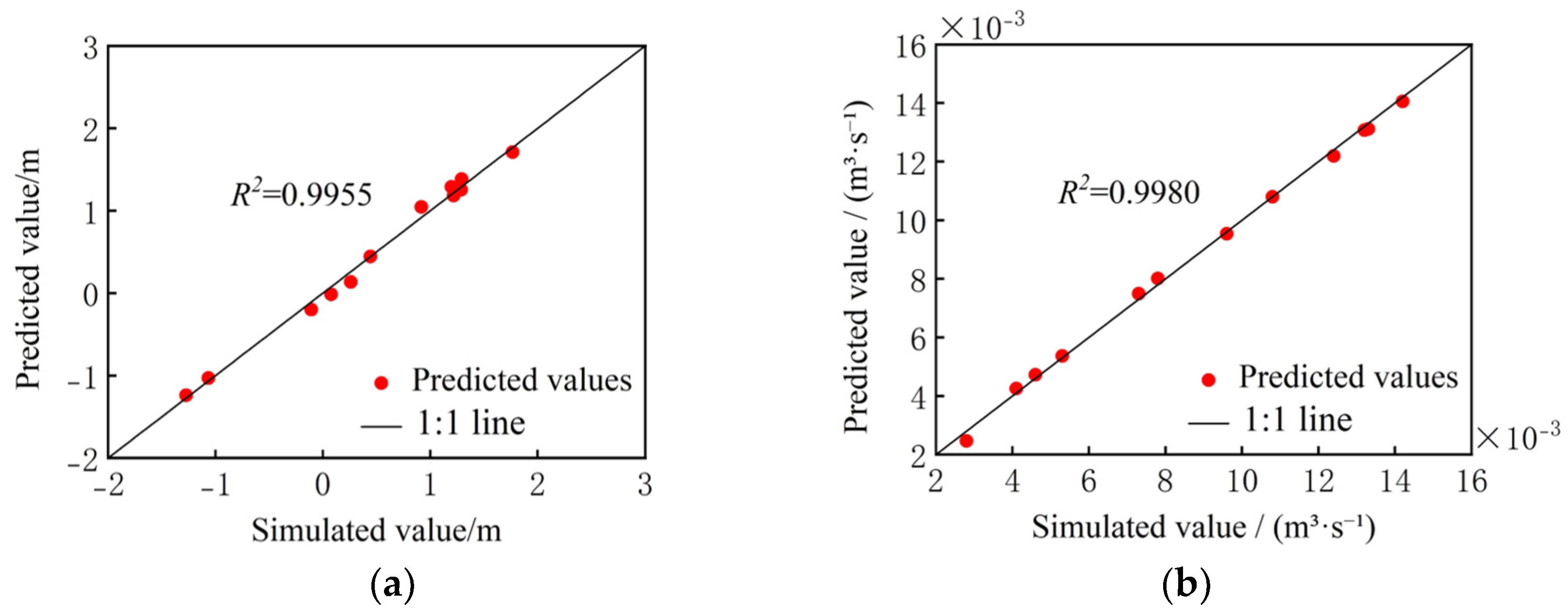
As shown in Figure 8, the predicted values of the relative uplift pressure head at the canal bottom and the single-well pumping rate were generally distributed close to the 1:1 line and showed good agreement with the finite-element simulation results. The coefficients of determination (R²) for the two models were 0.9955 and 0.9980, respectively, indicating that the fitted models accounted for 99.55% and 99.80% of the variability in the corresponding responses.

For the relative uplift pressure head model, the adjusted R² and predicted R² were 0.9896 and 0.9273, respectively, with a difference of 0.0623. For the single-well pumping rate model, the corresponding values were 0.9954 and 0.9676, with a difference of 0.0278. The relatively small differences between the adjusted and predicted R² values indicate that both models show good predictive consistency, with no strong evidence of overfitting.

Overall, the two response surface models provide satisfactory representations of the relationships between the design variables and the corresponding response indicators and are suitable for the subsequent response surface analysis and multi-objective optimization. Nevertheless, because the anti-uplift design is sensitive to small variations in the relative uplift pressure head near the allowable threshold, candidate designs close to this limit should be further verified using finite-element simulations.

3.3. Analysis of the Response Surface Results

3.3.1. Relative Uplift Pressure Head at the Canal Bottom

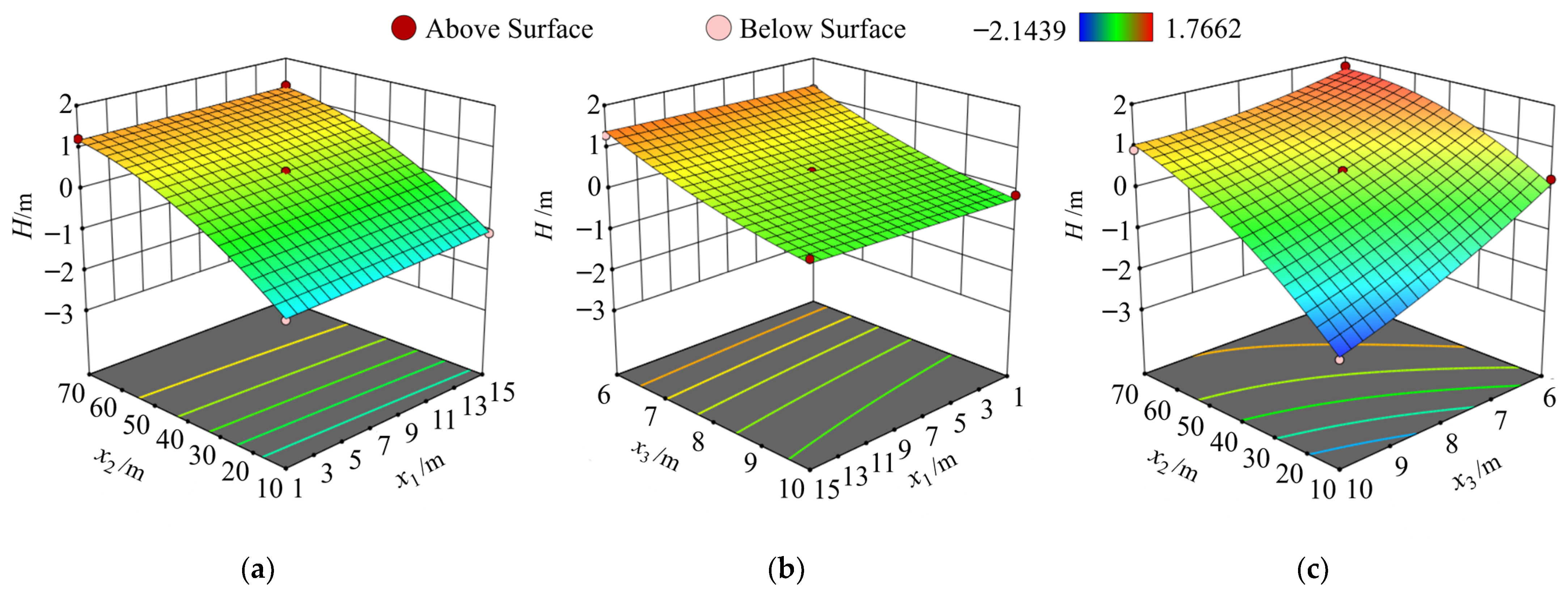
As shown in Figure 9, the relief-well spacing x₂ and the depth to the pumping control water level x₃ exert pronounced effects on the relative uplift pressure head at the canal bottom, whereas the influence of the horizontal distance from the relief wells to the canal edge x₁ is comparatively weak. This trend is consistent with the ANOVA results, which identified x₂, x₃, and the quadratic term $x_2^2$ as highly significant terms. When x₃ was fixed at 8 m, increasing x₂ from 10 to 70 m increased the relative uplift pressure head from approximately −1.0 to 1.0 m, indicating that a larger well spacing weakens the combined pressure-relief effect of adjacent wells. When x₂ was fixed at 40 m, increasing x₃ from 6 to 10 m resulted in an overall decrease in the relative uplift pressure head, because a greater depth to the pumping control water level corresponds to a lower controlled water level in the wells and therefore enhances groundwater drawdown.

When x₁ was fixed at 8 m, the combined variation in x₂ and x₃ produced a substantial change in the relative uplift pressure head. As the relief-well spacing increased from 10 to 70 m and the depth to the pumping control water level decreased to 6 m, the relative uplift pressure head increased from approximately −2.1 to 1.7 m, further demonstrating that larger well spacing and shallower depth to the pumping control water level are unfavorable for pressure relief.

Overall, the response-surface results indicate that the relative uplift pressure head is primarily controlled by the relief-well spacing and depth to the pumping control water level. Increasing the well spacing weakens the pressure-relief effect, whereas increasing the depth to the pumping control water level enhances groundwater drawdown. Therefore, appropriate combinations of x₂ and x₃ are required to maintain the uplift pressure below the prescribed anti-uplift limit.

3.3.2. Single-Well Pumping Rate

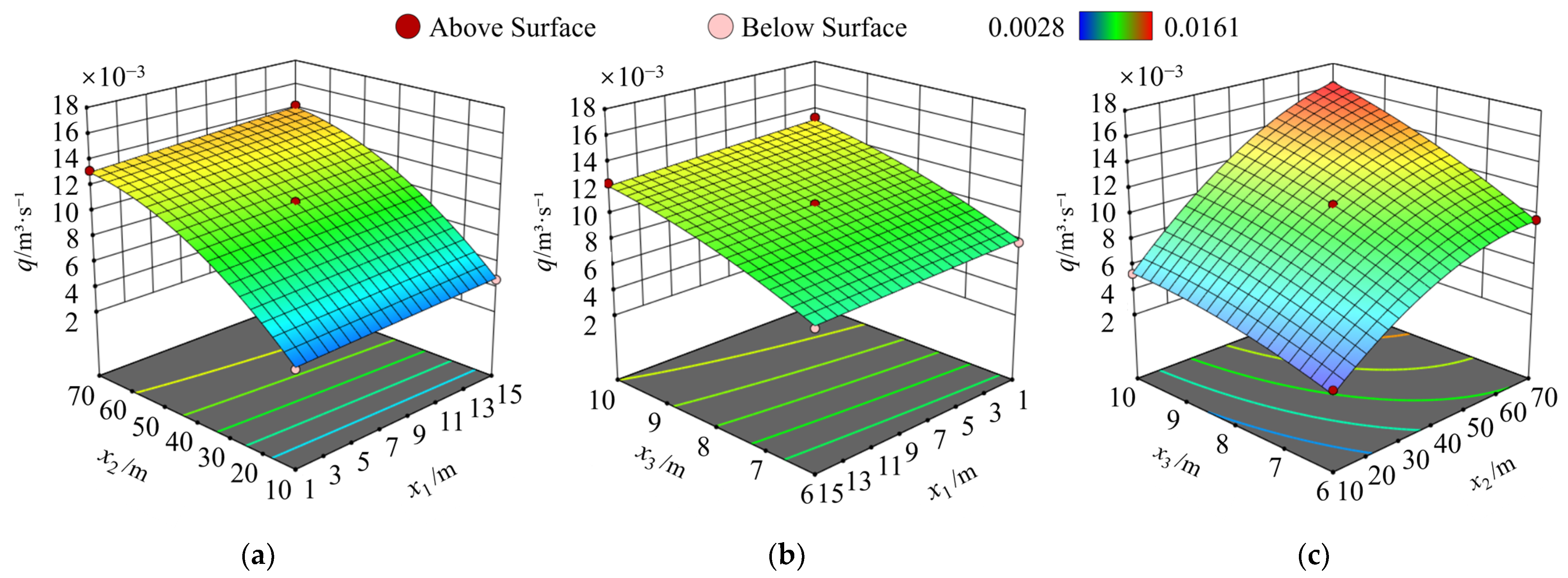
As shown in Figure 10, the relief-well spacing x₂ and the depth to the pumping control water level x₃ exert pronounced effects on the single-well pumping rate, whereas the influence of the horizontal distance from the relief wells to the canal edge x₁ is comparatively weak. This trend is consistent with the ANOVA results, which identified x₂, x₃, and the quadratic term $x_2^2$ as highly significant terms. When x₃ was fixed at 8 m, increasing x₂ from 10 to 70 m increased the single-well pumping rate from approximately 4 × 10⁻³ to 13 × 10⁻³ m³/s, indicating that a larger well spacing reduces the hydraulic interference between adjacent wells and enlarges the drainage area served by each individual well. When x₂ was fixed at 40 m, increasing x₃ from 6 to 10 m increased the single-well pumping rate from approximately 8.0 × 10⁻³ to 12 × 10⁻³ m³/s, because a greater depth to the pumping control water level corresponds to a lower controlled water level in the well and therefore produces greater drawdown and a larger hydraulic gradient toward the well.

When x₁ was fixed at 8 m, the combined variation in x₂ and x₃ produced a substantial change in the single-well pumping rate. As the relief-well spacing increased from 10 to 70 m while the depth to the pumping control water level decreased to 6 m, the single-well pumping rate increased from approximately 2.5 × 10⁻³ to 16.7 × 10⁻³ m³/s. This combined response reflects the competing effects of relief-well spacing and pumping-control depth on the pumping demand of an individual well.

Overall, wider well spacing reduces hydraulic interference between adjacent wells but increases the drainage load borne by each individual well, whereas a greater depth to the pumping control water level increases drawdown and consequently raises the single-well pumping rate. These trends indicate that the hydraulic benefits of pressure relief are accompanied by changes in well number and pumping demand, providing the basis for the subsequent multi-objective optimization.

3.4. Results of NSGA-II-Based Multi-Objective Optimization

To ensure the anti-uplift stability of the canal lining, the relative uplift pressure head at the canal bottom was constrained to remain below the allowable limit of 0.23 m above the canal-bottom slab during optimization. Subject to this constraint, the deviation of the relative uplift pressure head from the allowable threshold, F₁, the number of relief wells within the study reach, F₂, and the total pumping rate, F₃, were selected as the optimization objectives.

The relative uplift pressure head deviation was used to quantify the difference between the predicted head and the allowable threshold after the anti-uplift stability requirement had been satisfied. A smaller value indicates that the relative uplift pressure head is closer to the allowable limit, thereby avoiding the additional pumping demand associated with excessive groundwater drawdown. A smaller number of relief wells corresponds to a reduced construction scale, whereas a lower total pumping rate represents reduced operational pumping demand. Because the three objectives exhibit coupling and trade-offs, the Pareto front was used to characterize the compromises among them.

The optimization model expressed in Equation (8) was solved using the NSGA-II algorithm. The population size and maximum number of generations were set to 100 and 400, respectively, while the crossover and mutation probabilities were set to 0.9 and 0.33, respectively. During optimization, the relative uplift pressure head at the canal bottom and the single-well pumping rate of each candidate solution were first calculated using the response surface models. The number of relief wells and the total pumping rate within the study reach were then determined using Equations (6) and (7), respectively. Candidate solutions that failed to satisfy the anti-uplift stability constraint were discarded.

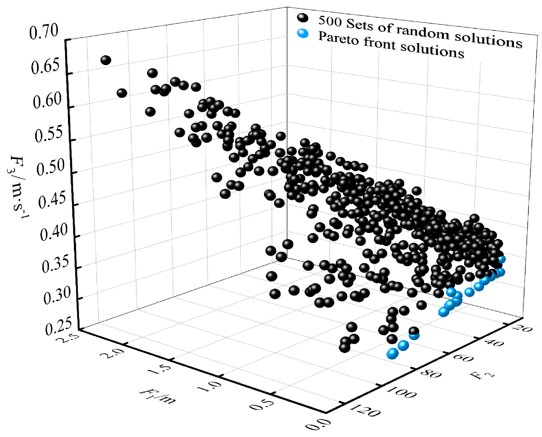
The NSGA-II optimization ultimately yielded 50 Pareto-optimal solutions, representing different trade-offs among the three optimization objectives. As shown in Figure 11, compared with the 500 randomly generated feasible solutions, the Pareto-optimal solutions were mainly distributed along the lower-value boundary of the feasible objective space, clearly illustrating the trade-offs among the competing objectives.

3.5. Hydraulic Conductivity Sensitivity Analysis and Determination of the Hydraulic-Conductivity Sensitivity Margin

Following the method described in Section 2.5.3, min–max normalization was first applied to the three objective functions of the 50 Pareto-optimal solutions. The geometric center of the Pareto solution set in the three-dimensional normalized objective space was then calculated as follows:

$$C=\left(0.1994 , 0.5453 , 0.4786\right)$$

The Euclidean distance between each Pareto-optimal solution and the geometric center was then calculated. The results showed that Solution ID 17 had the minimum distance to the geometric center. Therefore, it was selected as the intermediate representative solution P_M for the subsequent hydraulic conductivity sensitivity analysis. The corresponding design variables were x₁ = 1.0079 m, x₂ = 15.5401 m, and x₃ = 6.1761 m.

Based on this representative solution, finite-element seepage analyses were conducted for the single-factor perturbation scenarios S₀–S₆ defined in Table 5. The relative uplift pressure head at the canal bottom and its variation with respect to the baseline scenario S₀ are summarized in

Table 9. Hydraulic conductivity sensitivity results for the representative Pareto solution.

Scenario	Silty Clay K1/(m·s−1)	Silt–Fine Sand K2/(m·s−1)	Sand–Gravel Layer K3/(m·s−1)	H/m	$∆$H/m
S0	8.10 × 10−7	8.90 × 10−6	4.03 × 10−4	0.2284	0
S1	5.20 × 10−7	8.90 × 10−6	4.03 × 10−4	0.2284	0
S2	1.20 × 10−6	8.90 × 10−6	4.03 × 10−4	0.2284	0
S3	8.10 × 10−7	8.40 × 10−6	4.03 × 10−4	0.2284	0
S4	8.10 × 10−7	1.00 × 10−5	4.03 × 10−4	0.2285	0.0001
S5	8.10 × 10−7	8.90 × 10−6	6.00 × 10−5	0.2331	0.0047
S6	8.10 × 10−7	8.90 × 10−6	5.80 × 10−4	0.2282	−0.0002

.

The sensitivity analysis indicated that variations in the hydraulic conductivity of different soil layers have different effects on the relative uplift pressure head at the canal bottom. Among all perturbation scenarios, the change in the hydraulic conductivity of the sand–gravel layer produced the most pronounced hydraulic response. Under scenario S₅, the hydraulic conductivity of the sand–gravel layer decreased from 4.03 × 10⁻⁴ to 6.00 × 10⁻⁵ m/s, resulting in an increase in the relative uplift pressure head from 0.2284 m under the baseline scenario S₀ to 0.2331 m. The corresponding head increment was 0.0047 m, which was the maximum positive increment among all perturbation scenarios.

Accordingly, the maximum adverse head increment of 0.0047 m was adopted as the hydraulic-conductivity sensitivity margin, resulting in a sensitivity-adjusted screening threshold of 0.2253 m.

This adjusted threshold was subsequently used to screen the Pareto candidate solutions before the entropy-weighted TOPSIS evaluation.

3.6. Results of the Entropy-Weighted TOPSIS Evaluation

Table 10. Information entropy and entropy weights of the evaluation criteria for the sensitivity-screened Pareto candidate solutions.

Evaluation Criterion	Information Entropy	Entropy Weight
F1	0.9959	0.1879
F2	0.9914	0.3935
F3	0.9909	0.4186

presents the information entropy values and entropy weights of the evaluation criteria for the Pareto candidate solutions retained after sensitivity-based screening accounting for hydraulic conductivity uncertainty.

As shown in Table 10, the information entropy values of F₁, F₂, and F₃ are 0.9959, 0.9914, and 0.9909, respectively, with corresponding entropy weights of 0.1879, 0.3935, and 0.4186. Among the three criteria, F₃ has the largest weight, followed by F₂, whereas F₁ has the smallest weight. According to the entropy-weighting principle, a lower information entropy indicates greater differentiation among the candidate solutions and thus a larger contribution to the comprehensive evaluation. Therefore, the total pumping rate and the number of relief wells provide relatively stronger discrimination among the sensitivity-screened Pareto candidate solutions, whereas the relative uplift pressure head deviation contributes comparatively less to distinguishing the candidate solutions.

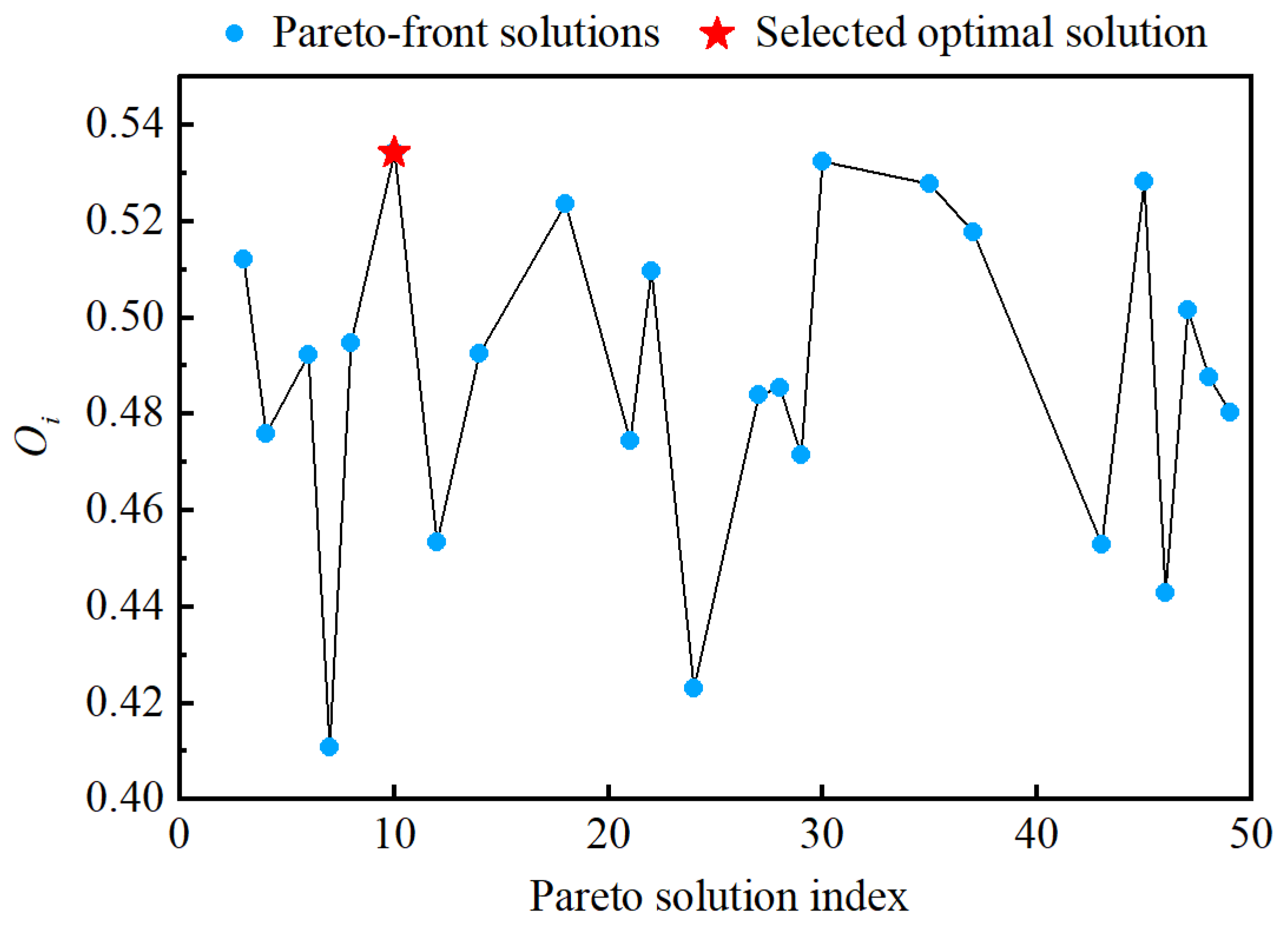
The relative closeness coefficients of the sensitivity-screened Pareto candidate solutions are shown in Figure 12.

According to the entropy-weighted TOPSIS results presented in Figure 12, candidate solution No. 10 exhibited the highest relative closeness coefficient (O_i = 0.5344) and was therefore selected as the optimal compromise solution. The predicted relative uplift pressure head of the selected solution was below the sensitivity-adjusted screening threshold of 0.2253 m, while the solution achieved a favorable balance among the relative uplift pressure head deviation, the number of relief wells, and the total pumping rate. The corresponding optimal design parameters were determined as follows: the horizontal distance from the relief wells to the canal edge was 1.95 m, the relief-well spacing was 38.8 m, and the depth to the pumping control water level was 8.36 m.

3.7. Results of the TOPSIS Weight Sensitivity Analysis

To evaluate the robustness of the entropy-weighted TOPSIS ranking to variations in the criterion weights, Monte Carlo random perturbations were applied to the baseline entropy weights, with perturbation ranges of ±10% and ±20%. The stability of the original optimal solution was assessed using the Top-1 rate, Top-3 rate, mean rank, and mean Spearman rank correlation coefficient (ρ), as summarized in

Table 11. Ranking stability under Monte Carlo random weight perturbations.

Weight Perturbation Range	Top-1 Rate/%	Top-3 Rate/%	Mean Rank	Mean ρ
±10%	84.33	87.73	1.8398	0.9067
±20%	56.55	71.29	3.9981	0.7390

.

Under ±10% weight perturbations, the originally selected solution remained ranked first in 84.33% of the simulations and remained within the top three in 87.73%, with a mean rank of 1.8398 and a mean Spearman rank correlation coefficient of 0.9067. These results indicate a high degree of consistency with the baseline TOPSIS ranking under moderate weight variations.

When the perturbation range increased to ±20%, the Top-1 and Top-3 rates decreased to 56.55% and 71.29%, respectively, while the mean rank increased to 3.9981 and the mean Spearman coefficient decreased to 0.7390. This decline indicates that the ranking becomes more sensitive as the magnitude of weight uncertainty increases. Nevertheless, the originally selected solution remained within the top three in more than 70% of the simulations, and the overall ranking remained positively correlated with the baseline ranking. Overall, the Monte Carlo analysis supports the robustness of the entropy-weighted TOPSIS decision under moderate weight perturbations, while also indicating increased ranking uncertainty under larger perturbations.

3.8. Finite-Element Verification of the Optimized Scheme

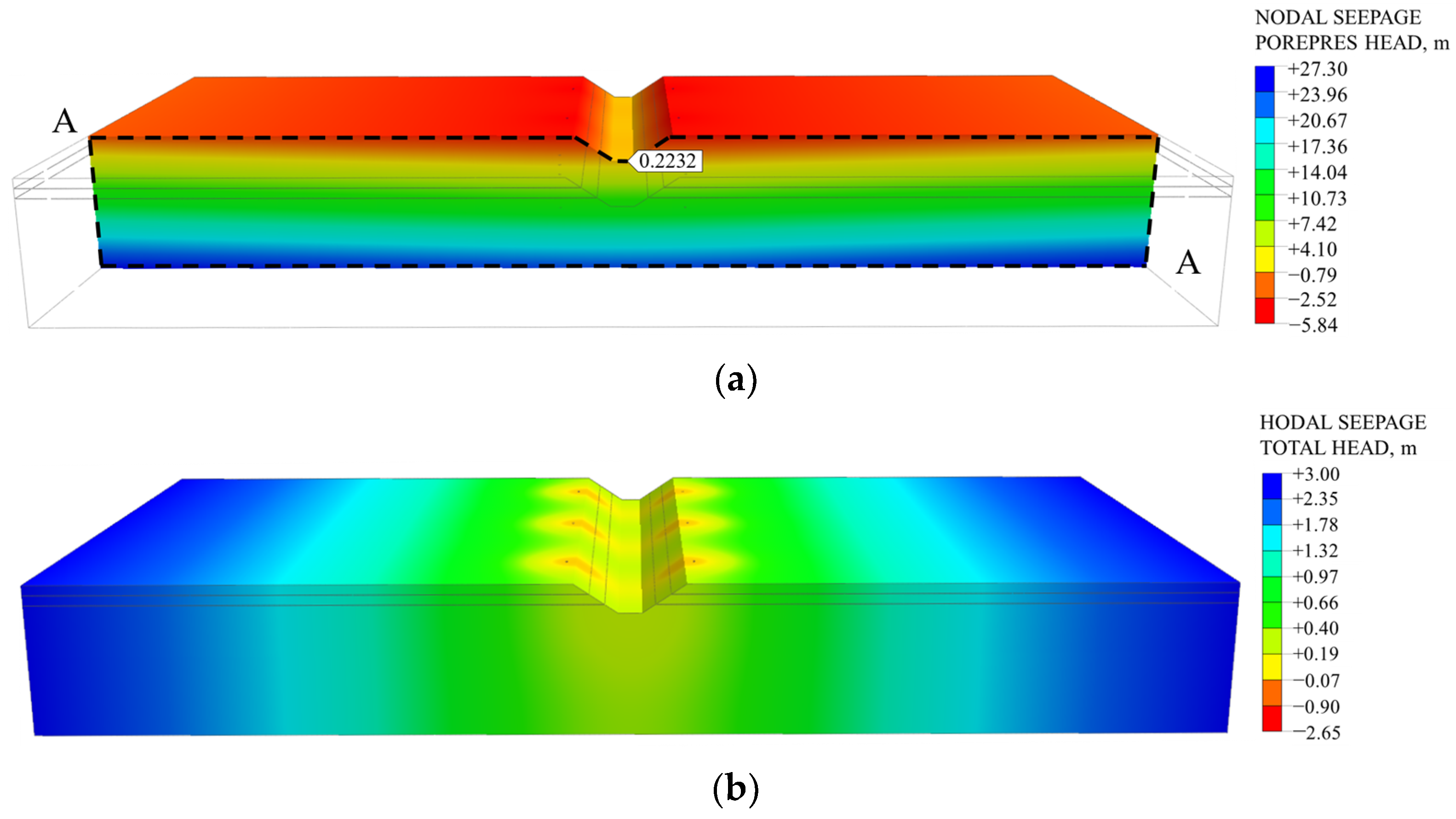
To independently verify the optimized dewatering scheme, a finite-element simulation was conducted using the selected design parameters. The simulation results are presented in Figure 13. The finite-element simulation yielded a relative uplift pressure head of 0.2232 m at the center of the canal bottom along the A–A control section, and a total pumping rate of 0.3462 m³/s.

A comparison between the response surface predictions and finite-element simulation results is presented in

Table 12. Comparison between the predicted and finite-element simulated values for the optimized scheme.

Indicator	Predicted Value	Finite-Element Simulated Value	Absolute Error	Relative Error (%)
H/m	0.2078	0.2232	0.0154	6.9
Q/(m3·s−1)	0.3456	0.3462	0.0006	0.17

. The predicted relative uplift pressure head and total pumping rate were 0.2078 m and 0.3456 m³/s, respectively. The corresponding absolute differences from the finite-element results were 0.0154 m and 0.0006 m³/s, equivalent to relative differences of 6.90% and 0.17%, respectively. The comparison also provides a direct finite-element check of the response-surface prediction for the selected scheme.

The finite-element simulation yielded a relative uplift pressure head below the sensitivity-adjusted screening threshold of 0.2253 m and the allowable anti-uplift limit of 0.23 m under the adopted design conditions. Meanwhile, the close agreement in the total pumping rate between the response surface prediction and finite-element simulation supports the reliability of the pumping-demand estimate for the selected scheme.

4. Discussion

Under high-groundwater conditions, the anti-uplift stability of canal linings is governed by the interaction between the groundwater seepage field and the hydraulic loading acting beneath the lining. In the investigated reach, deterioration of the existing subsurface drainage system reduced its pressure-relief capacity and contributed to lining heaving, cracking, and local sliding. By combining field monitoring, three-dimensional finite-element seepage analysis, response surface methodology, and multi-objective optimization, this study provides a systematic approach for determining relief-well design parameters.

The response surface analysis showed that relief-well spacing and the depth to the pumping control water level were the principal factors affecting both the relative uplift pressure head and the single-well pumping rate, whereas the horizontal distance from the wells to the canal edge had a comparatively limited influence. This behavior is consistent with the hydraulic role of the sand–gravel layer as the principal groundwater-transmitting stratum. Increasing well spacing reduces the overlap between the drawdown zones of adjacent wells and weakens the combined pressure-relief effect, while increasing the depth to the pumping control water level produces greater drawdown and lowers the uplift pressure beneath the canal lining. However, the latter also increases the pumping rate required from individual wells. These coupled responses indicate that maximizing groundwater drawdown is not necessarily desirable; instead, well spacing and depth to the pumping control water level should be coordinated to achieve adequate pressure relief without unnecessary pumping demand.

The NSGA-II optimization further demonstrated the trade-offs among hydraulic safety, relief-well construction scale, and total pumping demand. The resulting Pareto set provides a range of feasible alternatives representing different trade-offs among these objectives, thereby avoiding the limitations of a single-objective design and providing a clearer basis for selecting an appropriate relief-well configuration.

Hydraulic conductivity uncertainty is particularly important when candidate solutions approach the allowable uplift-pressure limit. The sensitivity analysis showed that variations in the hydraulic conductivity of the sand–gravel layer produced the most pronounced response. The most adverse perturbation increased the relative uplift pressure head by 0.0047 m, and this increment was adopted as the uncertainty-related hydraulic-conductivity sensitivity margin. Accordingly, a sensitivity-adjusted screening threshold of 0.2253 m was established for Pareto-solution screening. The resulting threshold provides a sensitivity-adjusted basis for screening the Pareto solutions before comprehensive decision-making.

After sensitivity-based screening, entropy-weighted TOPSIS was used to identify the compromise solution. The Monte Carlo weight sensitivity analysis showed that the selected solution retained the first rank in 84.33% of the simulations under ±10% weight perturbations, with a mean Spearman rank correlation coefficient of 0.9067. Under ±20% perturbations, the Top-1 rate decreased to 56.55%, although the solution remained within the top three in 71.29% of the simulations. These results indicate that the decision is relatively stable under moderate weight variations but becomes more sensitive as weight uncertainty increases. Overall, the selected solution exhibited good ranking stability under moderate weight perturbations, while larger perturbations resulted in increased ranking variability.

Direct finite-element verification of the selected scheme yielded a relative uplift pressure head of 0.2232 m and a total pumping rate of 0.3462 m³/s. The corresponding relative differences from the response surface predictions were 6.90% and 0.17%, respectively. The verified relative uplift pressure head remained below the sensitivity-adjusted screening threshold of 0.2253 m under the adopted design conditions.

Several limitations should nevertheless be recognized. The core optimization framework is based on steady-state seepage conditions, and rainfall infiltration, time-varying groundwater recharge, and other transient processes were not incorporated directly into the optimization loop. In addition, the hydraulic conductivity analysis adopted one-factor-at-a-time perturbations within prescribed parameter ranges and therefore does not represent a full probabilistic characterization of spatial heterogeneity or parameter correlation. Although cross-condition validation provided an independent check of the inverted hydraulic conductivity parameters, additional long-term monitoring under a wider range of hydraulic conditions would further strengthen model validation. The cross-condition validation errors also indicate that predictive accuracy may vary across hydraulic conditions, warranting further validation under a broader range of field conditions. Future work could integrate probabilistic parameter uncertainty, transient hydrogeological forcing, field performance monitoring, and explicit investment, energy, and maintenance costs into the optimization framework.

5. Conclusions

Based on the field-monitoring analysis, finite-element seepage simulations, response surface modeling, multi-objective optimization, uncertainty analysis, and finite-element verification, the main conclusions are as follows:

• A three-dimensional finite-element seepage model and quadratic response surface models were established for the relief-well dewatering system. Cross-condition validation provided an independent check of the hydraulic conductivity parameter set. The predicted R² values of the relative uplift pressure head and single-well pumping rate models were 0.9273 and 0.9676, respectively.
• Relief-well spacing and the depth to the pumping control water level were the dominant design factors affecting both the relative uplift pressure head and single-well pumping rate, with a significant interaction between them. Increasing well spacing weakened the combined pressure-relief effect, whereas increasing depth to the pumping control water level enhanced groundwater drawdown but increased the pumping demand of individual wells. The distance from the relief wells to the canal edge had a comparatively limited influence.
• Hydraulic conductivity sensitivity analysis identified the sand–gravel layer as the most influential soil layer among those investigated. The maximum adverse increase in the relative uplift pressure head was 0.0047 m. Taking this increment as the uncertainty-related hydraulic-conductivity sensitivity margin resulted in a sensitivity-adjusted screening threshold of 0.2253 m, which was used to pre-screen the Pareto candidate solutions before TOPSIS evaluation.
• Entropy-weighted TOPSIS selected a compromise design with a well-to-canal-edge distance of 1.95 m, a relief-well spacing of 38.8 m, a depth to the pumping control water level of 8.36 m, and 32 relief wells. Monte Carlo weight sensitivity analysis showed that the ranking was stable under moderate weight perturbations, while greater ranking variability occurred under larger perturbations. Finite-element verification yielded a relative uplift pressure head of 0.2232 m and a total pumping rate of 0.3462 m³/s, with the verified head remaining below the sensitivity-adjusted screening threshold and the selected scheme providing a reasonable balance among hydraulic safety, construction scale, and pumping demand.

References

1. Su, X.; Wei, K.; Hao, Z.J. Causes of lining instability of large water diversion channel and the effects of prevention and control measures. J. Chang. River Sci. Res. Inst. 2025, 42, 188–193. [Google Scholar] [CrossRef]
2. Tong, J.; Rao, X.B.; Quan, Q. Analysis of failure types and causes of multiple lining structures in water conveyance canals. Yangtze River 2021, 52, 168–171. [Google Scholar] [CrossRef]
3. Mansuri, B.; Salmasi, F.; Oghati, B. Effect of location and angle of cutoff wall on uplift pressure in diversion dam. Geotech. Geol. Eng. 2014, 32, 1165–1173. [Google Scholar] [CrossRef] [Scilit]
4. Jafari, F.; Salmasi, F.; Abraham, J. Numerical investigation of granular filter under the bed of a canal. Appl. Water Sci. 2019, 9, 137. [Google Scholar] [CrossRef] [Scilit]
5. Tian, M.; Chen, S.P.; Guo, X.L. Study on seepage control measures combining seepage prevention and drainage for hannan yangtze main levee. Rural Water Hydropower China 2024, 8, 161–168. [Google Scholar] [CrossRef]
6. An, A.-W.; Tian, M.; Wang, W.-Y. Random forest-based multi-objective optimization design method of relief wells for levee safety. Appl. Sci. 2025, 15, 11494. [Google Scholar] [CrossRef] [Scilit]
7. Tian, M.; Fan, H.; An, A.; Sheng, X. Relief well pumping strategy for levee safety based on multivariate adaptive regression splines (MARS) and non-dominated sorting genetic algorithm II (NSGA-II). Sci. Rep. 2025, 15, 40742. [Google Scholar] [CrossRef] [Scilit] [PubMed]
8. Fell, R.; Fry, J.J. Internal Erosion of Dams and Their Foundations: Selected and Reviewed Papers from the Workshop on Internal Erosion and Piping of Dams and Their Foundations, Aussois, France, 25–27 April 2005, 2nd ed.; CRC Press: Boca Raton, FL, USA, 2007. [Google Scholar]
9. Yao, Q.H.; Xu, C.; Xu, W.B. Transient antiseepage analysis of the relief well in Beijiang Dike. Math. Probl. Eng. 2020, 9, 7623481. [Google Scholar] [CrossRef] [Scilit]
10. Keffer, A.M.; Guy, E.D.; Grote, K.R. Finite line relief well system design for dams and levees. In Proceedings of the Geo-Congress 2023, Reston, VA, USA, 12–15 March 2023; American Society of Civil Engineers: Reston, VA, USA, 2023; pp. 31–48. [Google Scholar] [CrossRef] [Scilit]
11. Liu, C.S. Influence of relief well arrangement on levee seepage control. Rural Water Hydropower China 2001, 12, 64–66. [Google Scholar]
12. Zhang, H.; Shen, Z.Z.; Li, C.L. Study on seepage characteristics of flood diversion levee and arrangement scheme of relief wells. Adv. Water Resour. Hydropower Sci. 2010, 30, 67–69. [Google Scholar]
13. Keffer, A.M.; Guy, E.D. Relief wells for dams and levees considering landward head. J. Geotech. Geoenviron. Eng. 2023, 149, 04023092. [Google Scholar] [CrossRef] [Scilit]
14. Li, J.J.; Yang, Y.; Duan, X.B. Numerical analysis of factors affecting the performance of relief wells. J. Yangtze River Sci. Res. Inst. 2016, 33, 151–154. [Google Scholar] [CrossRef]
15. Chen, S.H.; Wang, B.; Fang, P.B. Study on combined pipe and well drainage and relief effect in high groundwater level canal sections. Rural Water Hydropower China 2022, 9, 36–43. [Google Scholar]
16. Zhao, Y.R.; Wang, H.N.; Xu, L.J. Solution and application of optimal dewatering model for foundation pits based on objective function method. People’s Yellow River 2023, 45, 136–142. [Google Scholar] [CrossRef]
17. Chen, Y.H.; Tsai, F.T.C.; Jafari, N.H. Multiobjective optimization of relief well operations to improve levee safety. J. Geotech. Geoenviron. Eng. 2021, 147, 04021041. [Google Scholar] [CrossRef] [Scilit]
18. Mirzaee, M.; Safavi, H.R.; Taheriyoun, M.; Rezaei, F. Multi-objective optimization for optimal extraction of groundwater from a nitrate-contaminated aquifer considering economic-environmental issues: A case study. J. Contam. Hydrol. 2021, 241, 103806. [Google Scholar] [CrossRef] [Scilit] [PubMed]
19. Jadid, R.; Montoya, B.M.; Bennett, V. Effect of repeated rise and fall of water level on seepage-induced deformation and related stability analysis of princeville levee. Eng. Geol. 2020, 266, 105458. [Google Scholar] [CrossRef] [Scilit]
20. EM 1110-2-1914; Design, Construction, and Maintenance of Relief Wells. U.S. Army Corps of Engineers: Washington, DC, USA, 2025.
21. DS-13(8)-4.1; Design Standards No. 13: Embankment Dams, Chapter 8: Seepage. U.S. Bureau of Reclamation: Denver, CO, USA, 2014.
22. Preene, M.; Roberts, T.O.L.; Powrie, W. Groundwater Control: Design and Practice, 2nd ed.; CIRIA C750; CIRIA: London, UK, 2016. [Google Scholar]
23. Middlebrooks, T.A.; Jervis, W.H. Relief Wells for Dams and Levees. Trans. Am. Soc. Civ. Eng. 1947, 112, 1321–1338. [Google Scholar] [CrossRef] [Scilit]
24. Bennett, P.T.; Barron, R.A. Design Data for Partially Penetrating Relief Wells. In Proceedings of the 4th International Conference on Soil Mechanics and Foundation Engineering; Butterworths Scientific Publications: London, UK, 1957; Volume 2, pp. 282–285. [Google Scholar]
25. Sharma, S.N.P. Partially penetrating multiple-well system in a confined aquifer with application to a relief well design. J. Hydrol. 1974, 23, 1–37. [Google Scholar] [CrossRef] [Scilit]
26. Mansur, C.I.; Postol, G.; Salley, J.R. Performance of Relief Well Systems along Mississippi River Levees. J. Geotech. Geoenviron. Eng. 2000, 126, 727–738. [Google Scholar] [CrossRef] [Scilit]
27. Batool, A.; VandenBerge, D.R.; Brandon, T.L. Practical Application of Blanket Theory and the Finite-Element Method to Levee Underseepage Analysis. J. Geotech. Geoenviron. Eng. 2015, 141, 04015001. [Google Scholar] [CrossRef] [Scilit]
28. Lu, Y.C. Design of intake canal for special geological section of HLJ hydropower station. Water Sci. Eng. Technol. 2018, 1, 56–59. [Google Scholar] [CrossRef]
29. SL 725-2024; Design Specification for Safety Monitoring in Water and Hydropower Projects. Standardization Administration of China: Beijing, China, 2024.
30. SL 551-2024; Technical Specification for-Earth-Rockfill Dam Safety Monitoring. Standardization Administration of China: Beijing, China, 2024.
31. Yan, T.Y.; Ren, J.J.; Liu, S.Z. Inversion of permeability coefficients of canal foundation soils under geomembrane defect conditions based on LHS-IGWO-RF. Water Resour. Power 2026, 1–12. Available online: https://link.cnki.net/urlid/42.1231.TK.20260611.1025.024 (accessed on 15 July 2026).
32. SL 265-2016; Design Specifications for Sluices. Standardization Administration of China: Beijing, China, 2016.
33. Huang, Y.C.; Xu, Y.Q. Numerical simulation analysis of dewatering and recharge process of deep foundation pits. Chin. J. Geotech. Eng. 2014, 36, 209–303. [Google Scholar] [CrossRef]
34. Li, Z.; Luo, Z.J.; Lu, J.S. Study on the impact of horizontal bottom sealing dewatering on the foundation pit surrounding environment. Chin. J. Undergr. Space Eng. 2025, 21, 1076–1084. [Google Scholar] [CrossRef]
35. Pei, C.K.; Wei, B.Q.; Chen, S.K. Analysis of seepage field based on improved node virtual flow method in a large-scale canal project during construction period. Hydro-Sci. Eng. 2017, 6, 22–28. [Google Scholar] [CrossRef]
36. GB 50296-2014; Technical Code for Tube Well. Standardization Administration of China: Beijing, China, 2014.
37. Shi, C.G.; Jiang, J.; Lei, M.F. Optimal design of construction dewatering of underground engineering with the consideration of dynamic dewatering process. J. Railw. Sci. Eng. 2017, 8, 1597–1605. [Google Scholar] [CrossRef]
38. Box, G.E.P.; Behnken, D.W. Some new three-level designs for the study of quantitative variables. Technometrics 1960, 2, 455–475. [Google Scholar] [CrossRef]
39. Deb, K.; Pratap, A.; Agarwal, S.; Meyarivan, T. A fast and elitist multiobjective genetic algorithm: NSGA-II. IEEE Trans. Evol. Comput. 2002, 6, 182–197. [Google Scholar] [CrossRef] [Scilit]
40. Hwang, C.-L.; Yoon, K. Multiple Attribute Decision Making: Methods and Applications—A State-of-the-Art Survey; Lecture Notes in Economics and Mathematical Systems; Springer: Berlin/Heidelberg, Germany, 1981; Volume 186. [Google Scholar] [CrossRef] [Scilit]
Figure 1. Study area location and representative canal-lining damage caused by groundwater uplift pressure.
Sustainability 18 09174 g001
Figure 2. Schematic cross-section of the canal structure and geological conditions.
Sustainability 18 09174 g002
Figure 3. Layout of groundwater, canal-water-level, and lining-deformation monitoring points along the K0 + 350–K0 + 970 canal reach.
Sustainability 18 09174 g003
Figure 4. Cross-sectional layout of piezometers and crack gauges at the representative damaged section at chainage K0 + 530.
Sustainability 18 09174 g004
Figure 5. Force diagram for the anti-uplift stability analysis of the canal lining.
Sustainability 18 09174 g005
Figure 6. Three-dimensional seepage model of the canal and finite-element mesh.
Sustainability 18 09174 g006
Figure 7. Flowchart of the optimization procedure for the relief-well dewatering system.
Sustainability 18 09174 g007
Figure 8. C. parison of predicted and finite-element simulated values for the response surface models: (a) Relative uplift pressure head, H; (b) Single-well pumping rate, q.
Sustainability 18 09174 g008
Figure 9. Response surfaces of the relative uplift pressure head at the canal bottom: (a) Combined effects of x1 and x2 on H; (b) Combined effects of x1 and x3 on H; (c) Combined effects of x2 and x3 on H. Dark-red and light-red markers represent the finite-element results from the Box–Behnken design runs located above and below the fitted response surface, respectively; the projected curves on the bottom plane represent contours of the fitted response surface.
Sustainability 18 09174 g009
Figure 10. Response surfaces of the single-well pumping rate: (a) Combined effects of x1 and x2 on q; (b) Combined effects of x1 and x3 on q; (c) Combined effects of x2 and x3 on q. Dark-red and light-red markers represent the finite-element results from the Box–Behnken design runs located above and below the fitted response surface, respectively; the projected curves on the bottom plane represent contours of the fitted response surface.
Sustainability 18 09174 g010
Figure 11. Three-objective Pareto front for the canal dewatering scheme.
Sustainability 18 09174 g011
Figure 12. Relative closeness coefficients of the sensitivity-screened Pareto candidate solutions.
Sustainability 18 09174 g012
Figure 13. Finite-Element verification of the optimized dewatering scheme: (a) Pore-pressure head distribution along the A–A control section; (b) Total-head distribution in the optimized dewatering scheme.
Sustainability 18 09174 g013