The Income Distribution and Poverty Effects of Industry-Differentiated Carbon Tax in China: A Study Based on the CGE-MS Approach

Abstract

As a market-based and cost-effective policy instrument for steering economies toward a more sustainable and low-carbon future, carbon tax has gained widespread attention globally. Nevertheless, introducing carbon tax in developing economies remains highly controversial due to potential adverse impacts on microeconomic agents, particularly concerning poverty and income inequality. Using data from the China Family Panel Studies, this paper characterizes the behavioral responses of micro-level agents and adopts a Computable General Equilibrium (CGE) model combined with Micro Simulation (MS) approach to dynamically simulate the behavioral reactions of individuals and households after the implementation of carbon tax in China from 2025 to 2035. The results show that: (1) Implementing an industry-differentiated carbon tax in China will not be regressive, and the public need not be concerned about the resurgence of poverty; (2) Carbon tax exerts stronger adverse impacts on high-income groups than on low-income households, thereby facilitating income equity; (3) Although allocating carbon tax revenue to subsidize the clean power generation sector can further narrow income gap, it concurrently leads to a reduction in resource allocation efficiency. By combining targeted social protection policies such as energy assistance and benefit compensation, government can minimize the negative impacts of carbon tax on vulnerable groups.

1. Introduction

Against the backdrop of deepening global climate governance, internalizing the externality of carbon emissions has become a core mechanism for achieving carbon neutrality. Market-oriented environmental policies, including carbon taxes and Emissions Trading Systems (ETS), raise the relative costs of high-carbon activities and guide the flow of capital and labor toward low-carbon sectors, which have evolved into mainstream decarbonization pathways worldwide. According to World Bank statistics, by 2025, 80 carbon pricing systems were operating globally, covering 28% of greenhouse gas emissions. Among them, there were 43 carbon tax schemes and 37 ETS programs, with new mechanisms concentrating in emerging market economies.

China launched regional ETS pilot programs in 2011 and established a national unified carbon market a decade later, initially covering only the power sector. In 2025, China expanded its national carbon market to include three major energy-intensive industries: iron and steel, cement, and aluminum smelting. It further announced its intention for the national ETS to cover major emitting sectors within the industrial domain by 2027. According to statistics from China’s Ministry of Ecology and Environment, by the end of 2025, the cumulative trading volume of carbon allowances in the national carbon market had reached 865 million tons, with a cumulative turnover of CNY 57.663 billion. From a timeline perspective, after five years of operation, the ETS has completed a full cycle of evolution from institutional establishment to stable operation, and from single-industry to multi-industry coverage. A fundamental consensus on the principle of carbon pricing has been formed among both the public and enterprises, providing an optimal institutional window of opportunity for the introduction of carbon taxes. Additionally, the EU’s Carbon Border Adjustment Mechanism (CBAM) officially takes effect in 2026. As a sovereign taxation regime, carbon tax is more recognizable and mutually acknowledged in international carbon pricing practices compared with ETS. In line with the principle of avoiding double taxation, carbon taxes levied by exporting countries can be credited against the CBAM. Therefore, introducing a carbon tax in China will not only compensate for the ETS’s limited coverage and liquidity but will also serve as a strategic choice to safeguard national tax interests and build a comprehensive climate governance system.

From the perspective of institutional structure, carbon tax and ETS are mutually complementary. ETS ensures emission reduction certainty via a cap-and-trade mechanism, while carbon tax stabilizes abatement costs through price signals. Specifically, centered on quantity control, ETS sets a rigid emission cap but is subject to price volatility, potentially destabilizing corporate investment in emission reduction. Carbon tax, centered on price control, sets a fixed rate to create a stable price signal but faces uncertainty in total emissions due to factors like technological elasticity and market response. At the level of institutional linkage, their coordination can overcome the inherent flaws of either instrument alone, achieving a Pareto improvement in both emission reduction efficiency and economic costs. On the one hand, carbon tax rate sets an implicit price floor for ETS and alleviates economic shocks caused by carbon price volatility. On the other hand, real abatement cost data generated by ETS provide a reference for the dynamic adjustment of carbon tax rate and lower the information barrier for policy design.

Despite the gradual expansion of China’s ETS, the high entry threshold of carbon markets limits their effectiveness for dispersed emission sources (e.g., the transportation sector) and Small and Medium-sized Enterprises (SMEs), potentially triggering carbon leakage risks. Therefore, imposing industry-differentiated carbon tax on industries already covered by ETS still retains practical significance. This policy can impose effective constraints on tens of thousands of SMEs that remain outside the scope of carbon market regulation, accurately covering the blind spots of ETS. In the long run, China still needs to launch a carbon tax at an appropriate time and coordinate it with ETS to jointly advance the goals of carbon peaking and carbon neutrality.

However, as a government regulatory tool, carbon tax inevitably reshapes the existing income distribution through price transmission mechanisms. After a carbon tax is levied, rising production costs may be passed forward to consumers via higher commodity prices or shifted backward to employees through reduced wages (the specific proportion depending on the demand and supply elasticities of products and factors), affecting household income distribution [1]. When the adverse impact of carbon tax on low-income households is proportionally greater than on high-income groups, the tax is regressive, exacerbating inequality and potentially pushing vulnerable groups below the poverty line [2]. Due to variations in countries, periods, and industries, the progressive/regressive nature of carbon taxes differs accordingly [3,4,5]. Therefore, the analysis of its income distribution and poverty effects requires a case-by-case approach.

For a large country like China, characterized by significant regional imbalances in resource endowments and development levels, the impacts of carbon tax on poverty and income distribution are particularly complex and constitute a critical issue in the decision to adopt one. China’s economy has transitioned from high-speed growth to high-quality development. Given the heterogeneity in policy effects across countries, industries, and periods, there is an urgent need to analyze the impacts of carbon tax on income distribution and poverty based on China’s current developmental stage and to propose compensatory mechanisms and protective policies for vulnerable groups to reduce policy implementation barriers.

This study integrates econometric microsimulation with the CGE model (CGE-MS) to identify the micro-agents (including individuals and households) affected by carbon taxes. By comparing changes in indicators such as poverty incidence, Gini coefficient, Growth Incidence Curve (GIC) and Sen index across multiple scenarios, it quantitatively assesses the impacts of an industry-differentiated carbon tax on poverty and income distribution. The main findings are as follows: (1) Over time, carbon tax does not reverse the declining trend in poverty but merely slows its rate of decrease; (2) China’s implementation of a carbon tax will be progressive, meaning that its impact on wealthy groups will be greater than that on the poor, thereby narrowing income gap; (3) Recycling carbon tax revenues to households mitigates the policy’s adverse poverty impacts. These findings support a dual-driver approach (“ETS + carbon tax”) in China to achieve the “dual carbon” goal.

This paper makes several contributions: (1) Methodologically, it innovatively introduces CGE-MS approach into the study of the income distribution effects of carbon taxation, incorporating industry heterogeneous tax rates into an integrated macro-micro analytical framework. By integrating the industrial linkage effects of a macro CGE model with household heterogeneity of microsimulation models, it captures the complex impacts of industry-differentiated carbon taxes (i.e., setting rates based on sectoral shadow prices of ${\mathrm{CO}}_2$) transmitted through industrial chains to different income groups. (2) Empirically, based on characterizing individual and household behavioral responses, it quantitatively evaluates the distributional effects of industry-differentiated carbon taxes across income groups, expanding the research boundary of social welfare. (3) Practically, by designing multiple revenue recycling mechanisms, it provides micro-level evidence for policymakers aiming to balance efficiency and equity and realize the “double dividend” of carbon taxation.

The remainder of this article is structured as follows. Section 2 reviews the relevant literature. Section 3 describes the model setup and data processing. Section 4 reports and discusses the changes in poverty incidence, Gini coefficient, GIC and Sen index under different scenarios, and finally Section 5 concludes with policy recommendations.

2. Literature Review

The choice of policy tools to address climate change is not only related to environmental effectiveness, but also deeply embedded in the balance between social equity and economic efficiency. Most existing studies focus on the progressive or regressive nature of carbon taxes when analyzing their micro-level impacts on households and individuals.

The conventional view holds that carbon pricing policies are inherently regressive. Low-income households spend a larger share of disposable income on energy-intensive goods and services such as heating and transportation, making them more vulnerable to price hikes induced by carbon taxes. Empirical studies from several countries partially support this view. For instance, Reaños and Lynch [6] adopt a flexible demand system and Irish household data to quantify the income distribution effects of carbon taxes, and find that reduced purchasing power constitutes the main source of welfare losses, with low-income rural households and retirees suffering the most severe impacts. If low-income groups cannot cut energy consumption, price increases driven by carbon taxes will hit them harder than affluent ones. Douenne and Fabre [7] document the regressive nature of France’s carbon tax, which penalizes rural and suburban households and triggers public discontent over declining purchasing power. Bureau [8] similarly points out that without tax revenue recycling, poorer households bear a higher carbon tax burden relative to their disposable income: the carbon tax accounts for nearly 1% of disposable income for the poorest 10% of households, compared with only 0.3% for the richest 10%. Research on various states and income groups in the United States, conducted by Williams et al. [9], also confirms that carbon taxes impose heavier burdens on low-income households in the absence of revenue recycling mechanisms.

Nevertheless, with more refined methodologies, this conclusion is not universal and exhibits heterogeneity across countries and industries. (1) At the national level, Metcalfe [10] find that when considering declining capital returns (wealth primarily held by high-income earners), the overall distributional effects of carbon taxes in the United States tend to be neutral or even progressive, rather than purely regressive. Studies on Chile [11], Brazil [12] and several European countries [13] suggest that carbon taxes may generate roughly proportional or even progressive distributional effects under specific conditions. Based on an ordered probit meta-analysis covering 53 carbon pricing studies (including 183 impacts from 39 countries), Ohlendorf et al. Ref. [14] demonstrates that carbon pricing tends to produce proportional or progressive effects on income distribution in developing economies. Given the divergent consumption patterns between developed and developing economies, Timilsina [15] argues that empirical conclusions from developed countries cannot be directly extrapolated to developing nations. (2) At the industrial level, Barker and Köhler [16] find that taxes on transportation fuels are mildly progressive, whereas taxes on residential energy tend to be regressive. Similarly, Tiezzi’s [17] research on Italy and Wang et al.’s [18] study on urban and rural households across Chinese provinces further verify the industrial heterogeneity of carbon tax, with the final distributional outcomes of carbon taxes being jointly determined by consumption patterns, factor income structures and indirect price transmission.

Given the potential inequities caused by carbon pricing, revenue recycling has become a critical measure to mitigate social conflicts and improve policy feasibility. Based on representative household data in France, Berry [19] simulates carbon taxes on residential heating and transportation fuels. The results show that carbon taxes are regressive and exacerbate fuel poverty without revenue redistribution, while recycling part of carbon tax revenues to households can offset inequality at a reasonable cost and help alleviate fuel poverty. For Austria, Kirchner et al. [20] use an input-output model to simulate carbon taxes on sectors excluded from the EU’s ETS, alongside three revenue recycling schemes: labor tax reduction, value-added tax reduction and lump-sum transfers. Their results indicate that carbon taxes are regressive without revenue recycling, and lump-sum transfers minimize the trade-off between equity and efficiency. Using a microsimulation model, Saelim [21] explores household demand responses to carbon taxes and finds that expanding social transfer programs and returning tax revenues via pension benefits reduce poverty rates and improve the welfare of the bottom income quintile. Empirical evidence from British Columbia [22], Switzerland [23], and Mexico [24] also shows that well-designed revenue recycling mechanisms can not only offset the adverse impacts of carbon taxes but even yield net benefits for low-income households.

Methodologically, research on the distributional effects of carbon taxes falls into three main categories: (1) CGE models with representative households, where the household sector is disaggregated into a few representative types (e.g., urban/rural, skilled/unskilled). This allows preliminary micro-level analysis but assumes homogeneous distribution within each group [25]. (2) CGE models with multiple households, where micro-household data from surveys are directly incorporated, treating each household as a distinct category. This method captures observed heterogeneity but does not model discrete behavioral choices of agents, potentially overestimating policy impacts [26]. (3) CGE models coupled with microsimulation (CGE-MS), where macro outcomes (e.g., prices, wages, employment) from the CGE model are fed into micro-behavioral equations to analyze impacts on household consumption, personal income, employment status, etc. [27,28].

With improved data availability and computational capabilities, recent studies increasingly use CGE-MS approach to overcome limitations of the others. This paper precisely adopts the method to analyze the progressive/regressive nature of industry-differentiated carbon taxes in China. Combining with three revenue recycling mechanisms (full subsidy to the clean power sector, full transfer to the household sector, and a mixed scheme with equal allocations to the two sectors), this study quantitatively examines the dynamic impacts of carbon taxes on income distribution and poverty from 2025 to 2035.

3. Theoretical Analysis

The equity of income distribution is not only a vital component of social fairness but also a focal issue of broad public concern. The imposition of carbon taxes may exert both positive and negative effects on household income distribution. On the one hand, as a fiscal instrument, carbon tax can mitigate income inequality through income redistribution mechanisms such as transfer payments. On the other hand, akin to environmental taxes, carbon tax may exhibit regressive distributional effects, whereby low-income households bear a disproportionately larger tax burden, thereby exacerbating income inequality. Specifically, carbon taxes affect micro-agents through the following three channels.

3.1. Consumption Channel

When levied on the production side, carbon taxes raise the cost of energy inputs. Firms respond by adjusting product prices, passing part or all of the tax burden on to consumers, thereby indirectly affecting household and individual consumption. In the short run, factor substitution is difficult to achieve, leaving firms with little option but to shift the tax burden via higher prices; the share borne by each party depends on the price elasticities of supply and demand. Ganapati et al. [29] estimate that, in the short-to-medium term, the average pass-through rate is approximately 70%, though it varies considerably across industries. In the long run, carbon taxes incentivize firms to enhance energy efficiency and transition toward low-carbon energy sources, thereby moderating its impact on production costs and consumer prices. Moreover, carbon taxation renders the development and adoption of new technologies economically viable, which can substantially reduce the long-run cost of carbon abatement. Thus, the adverse micro-level impacts of carbon taxes through indirect price effect are likely to diminish over time.

3.2. Income Channel

Following carbon tax implementation on productive sectors, firms adjust factor inputs in response to rising production costs, which in turn affects household and individual income levels.

3.2.1. Traditional Energy-Intensive Industries

Relative to service and high-tech industries, carbon-intensive sectors (such as energy production, mining, transportation, and heavy manufacturing) are more likely to reduce output and labor demand in response to carbon taxation. Given the high geographic concentration of traditional energy-intensive industries, these sectors often account for a large share of local employment. Consequently, the shutdown or downsizing of such firms may have persistent adverse effects on the employment and income of local residents. Additionally, the environmental degradation caused by fossil fuel extraction and power generation (such as landscape damage and waterway obstruction) can deter the entry of emerging industries and further deteriorating regional labor market conditions. Meanwhile, energy-intensive industries are typically capital-intensive as well. When these industries are replaced by labor-intensive sectors such as light manufacturing, the decline in capital returns is likely to exceed wage reductions. This implies that households deriving a larger share of total income from capital will suffer greater losses, demonstrating that the composition of income is also a crucial determinant of carbon tax distributional incidence.

3.2.2. Renewable Energy Industries

The implementation of carbon taxes renders the development and utilization of low-carbon energy sources (such as renewable energy) economically viable, thereby potentially increasing both investment and employment opportunities in these industries. For instance, Yamazaki [30] identifies a dramatic labor reallocation from carbon-intensive to low-carbon industries after British Columbia introduced its carbon tax. Since different sectors require distinct skill sets, labor productivity, and wage scales, sector-specific responses to employment shifts and wage adjustments also vary. Consequently, carbon taxes generate uneven income and employment shocks for different occupational groups, reshaping intra-household and individual income distribution. Marin and Vona [31] further observe that climate policy implementation triggers a labor market shift toward skilled technical workers at the expense of manual laborers, implying low-skilled workers may be the most adversely affected by carbon taxation.

3.3. Redistribution Channel

The manner in which carbon tax revenues are recycled is a critical component of policy design, aimed at balancing the trade-offs among emission reduction efficiency, economic development, poverty alleviation, and income equity. Typical revenue recycling schemes include tax relief, public investment, and transfer payments.

3.3.1. Firm-Oriented Recycling Policies

Nallareddy et al. [32] demonstrate that corporate income tax cuts exacerbate income inequality in the United States, as such taxes are largely borne by capital, and high-income individuals benefit disproportionately from these tax reductions compared to low-income workers. Empirical evidence suggests public investment (including green infrastructure spending) tends to compress income gaps in developing economies. However, its specific impact on micro-agents depends on multiple factors. If low-income households spend a relatively large share of their budgets on energy-intensive goods, green investment may improve their living standards by lowering energy prices. By contrast, investments in electric vehicles and charging infrastructure disproportionately benefit affluent households with higher rates of private EV ownership. Additional moderating factors include the geographic targeting of public investment, baseline wage levels of workers employed in recipient sectors, and the magnitude of cross-industry spillover effects, all of which shape the ultimate distributional outcomes of public spending policies.

3.3.2. Household-Oriented Recycling Policies

Gerber et al. [33] find that low-income households derive minimal gains from personal income tax reductions, given their limited income tax liabilities. Reallocating carbon tax revenues to upgrade public education and healthcare facilities in underdeveloped and impoverished communities expands disadvantaged households’ access to essential public services, reducing poverty and income stratification. Generally speaking, transfer payments are the most effective instrument for protecting vulnerable groups, with both universal and means-tested transfers effective in mitigating carbon tax burdens on households. While targeted transfers based on household economic status deliver superior cost-effectiveness, their implementation demands rigorous administrative capacity. In addition, governments can assist households in shifting toward low-carbon consumption. For example, providing affordable public transportation in areas with a high proportion of long-distance commuters, or subsidizing more energy-efficient stoves and lower-carbon heating systems. It should be noted that the effectiveness of any revenue recycling scheme depends on the overall performance of the policy combination, and governments should design comprehensive reform packages tailored to national socioeconomic realities.

4. Research Methodology

4.1. CGE Model

In the CGE model, producers make optimal input decisions and determine the optimal supply quantity based on the principle of maximizing profits under technical constraints; Consumers make optimal expenditure decisions and determine the optimal demand based on the principle of utility maximization under budget constraints; Equilibrium price ensures that the optimal supply and demand are equal, resources are effectively utilized, consumer utility is satisfied, and the economy reaches a stable equilibrium state. Then, external shocks are introduced into the steady state in the model, and when the economic system returns to equilibrium again, the changes in relevant variables are evaluated to analyze the impact of exogenous shocks.

Based on research needs, this paper makes the following modifications to the dynamic CGE model of China’s energy-environmental-economic analysis (CEEEA2.0) developed by Jia and Lin [34]: (1) adding a tax rate adjustment coefficient to the carbon tax module to achieve industry differentiated taxation; (2) Incorporate the carbon tax cost of the industrial sector into indirect taxes, and simulate government support for the clean power generation industry by reducing indirect taxes on enterprises; (3) Add carbon tax revenue to the direct tax equation and simulate the government transferring carbon tax revenue to the household sector through the reduction or exemption of direct taxes for residents. The specific model equations can be found in the Appendix A.1 and Shen et al. [35].

In terms of scenario design, the study sets up two sets of scenarios for policy simulation: The first set revolves around whether to impose an industry-differentiated carbon tax and the time interval for adjusting its rate, including three scenarios: BAU, FLX and STK. Among them, no carbon tax is levied in the business as usual scenario (BAU). Both the flexible tax rate scenario (FLX) and the sticky tax rate scenario (STK) implement carbon taxes to achieve the “dual carbon” goal. The tax rate is endogenously determined by preset emission reduction paths. The difference lies in that FLX scenario allows annual tax rate adjustments, while the STK scenario revises tax rate every five years.

The second set of scenarios is designed under the condition of imposing a sticky industry-differentiated carbon tax, focusing on different ways of using tax revenue, including four scenarios: STK, ENE, HOH, and MIX. Among them, all carbon tax revenues are retained by government in the STK scenario. The energy substitution scenario (ENE) allocates all revenues to subsidize the clean power sector, and the household welfare scenario (HOH) transfers all revenues directly to households. The mixed subsidy scenario (MIX) splits revenues equally between the household sector and the clean power sector. In the ENE scenario, carbon tax revenues are allocated in proportion to the output value of the clean electricity generation sector, thereby subsidizing the industry by offsetting corporate indirect taxes. In the HOH scenario, carbon tax revenues are distributed according to the ratio of urban to rural labor factor inputs, thereby subsidizing households by offsetting direct taxes on residents.

This paper dynamically simulates the micro-level impacts of an industry-differentiated carbon tax from 2025 to 2035, assuming key household characteristics (e.g., demographic structure, school enrollment) remain constant. According to the China Health Statistics Yearbook (2022), total population is projected to fall to 1.38 billion by 2035. Based on this projection, the article employs linear interpolation to obtain annual population and sample reweighting to match the yearly population totals.

4.2. MS Models

4.2.1. Occupational Choice Model

This study classifies occupations into four mutually exclusive categories: employed, self-employed, agricultural production and inactive (unemployed and apprentices). Due to the lack of data on secondary occupations, this study focuses solely on primary occupations, disregarding mixed employment situations (such as wage earners who are also self-employed employers). Workers are divided into skilled and unskilled groups with no cross-group mobility, but each worker can freely switch between different occupations according to their personal and family circumstances. Given that the labor market is currently characterized by imperfect competition, wage rates vary across different sectors, occupation types, and skill levels.

Due to the lack of relevant data on labor hours, this study posits that the labor supply of family members constitutes discrete choices among the aforementioned four occupations, with each choice satisfying the conditions for maximizing discrete utility. Therefore, this paper employs a standard multinomial logit model to estimate individual labor supply. The utility derived from engaging in a particular occupation is represented by a set of functions encompassing individual and family characteristics:

$$\ln {\displaystyle \frac{P\left(E_i=m\right)}{P\left(E_i=4\right)}}={\alpha }_m+{\sum }_{j=1}^J{\beta }_{mj}{X}_{ij}+u_{ij}=Z_{mi}$$

(1)

where, $Z_{mi}$ is the utility from occupation m for individual i. The career utility of the fourth category, which is unemployed, is set to 0, i.e., $Z_{4i}=0$. $X_{ij}$ is personal characteristic information of individual i in industry j. Referring to previous studies [17,36,37], variables such as occupation category, wage, household registration type, region, gender, head of household status, age, education, number of children, and marital status are selected. $u_{ij}$ is the individual residual term, which follows an independent and random distribution with a double-exponential form.

If ${\alpha }_m+{\beta }_m{X}_{im}+{\epsilon }_{im}>Max\left({\alpha }_s+{\beta }_s{X}_{is}+{\epsilon }_{is}\right)s=1,\dots ,M,\forall s\ne m$, then the individual i will choose to pursue the career m.

The model assumes that within a family, members choose occupations in a certain order: Household heads make occupational decisions first, followed by other family members. Therefore, this study first estimates the head of the household’s occupational choice based on general household and family member characteristics, and then estimates the polynomial logit model for other members based on the head of the household’s decision.

In each simulation period t, the probability of choosing each occupation is as follows:

Employment scenario: $P\left(E_i=m\right)={\displaystyle \frac{\exp \left(Z_{mi}\right)}{1+{\sum }_{m=1}^{m=3}\exp \left(Z_{mi}\right)}}$

Unemployment scenario: $P\left(E_i=4\right)={\displaystyle \frac{1}{1+{\sum }_{m=1}^{m=3}\exp \left(Z_{mi}\right)}}$

Based on this, the probability of selecting each occupation is estimated to reallocate individual employment status after policy shocks. According to the CGE results concerning the employment status, the absolute numbers moving in or out the four working categories is estimated. The individuals changing from one alternative to another are selected according to their probability of being in the concerned choice.

4.2.2. Personal Income Model

Wages at the individual level are typically estimated using the Heckman two-step method. Firstly, a Probit function is used to estimate the “choice equation”, which determines whether the individual i is employed. The equations take the following form:

$$s_i^{*}=\gamma z_i+u_i$$

(2)

$$s_i=\left\{\begin{array}{c}1,s_i^{*}>0\hfill \\ 0,s_i^{*}\le 0\hfill \end{array}\right.$$

(3)

where, $Z_i$ is an appropriate selection variable, which generally include marital status ($married$), age ($age$), gender ($gender$), region ($region$), number of children ($n\text{\_}children$). $u_i$ is an unobserved characteristic variable that affects individuals’ choice of whether to be employed. Next, labor income is estimated using the following equation:

$$w_i=\left\{\begin{array}{c}\beta x_i+{\epsilon }_i,s_i^{*}>0\hfill \\ ·,s_i^{*}\le 0\hfill \end{array}\right.$$

(4)

The selected control variables are: gender ($gender$), head of household status ($hh\text{\_}head$), region ($region$), age ($age$), and education level ($education$). ${\epsilon }_i$ represents unobserved individual characteristic variables, reflecting the heterogeneity of individual income. For non-employed individuals, reservation wages are drawn from the observed distribution of residuals for their skill level, allowing estimation of potential entry/exit thresholds. After an exogenous shock, individuals with highest reservation wages exit first if real wages fall; those with lowest reservation wages enter first if real wages rise. Changes in average wages (i.e., total payroll) with respect to the baseline figures in the MS models are equal to changes in wage rates obtained in the CGE model for each type of worker category.

4.2.3. Household Earnings Model

Household earnings from agricultural activities and self-employment, can be represented by the difference between the value of output and input over a specific period. Furthermore, the opportunity cost of the employer’s own participation in production must also be taken into account and its value estimated at market prices. This article assumes that the basic model of household income follows the Cobb-Douglas function form. After taking the logarithm of all variables, it can be obtained:

$$\ln {\Pi }_{h,t}^j=\alpha +{\beta }_1\ln X_{h,t}+\beta \ln N_{h,t}^{j,sk}+{\beta }_3\ln N_{h,t}^{j,unsk}+u_h$$

(5)

$$N_{h,t}^{j,sk/unsk}={\sum }_{i=1}^{N}I\left(E_{i,t}^{sk/unsk}=j\right)$$

(6)

where $E_{i,t}^{sk/unsk}$ represents occupational choices, $j=2$ represents the non-agricultural self-employment sector, and $j=3$ represents the agricultural production sector. $N_{h,t}^{j,sk}$ and $N_{h,t}^{j,unsk}$ are respectively denote the number of skilled and unskilled household workers in period t. $X_{h,t}$ is used to identify household characteristics, mainly including household registration type ($urban$), region ($region$), gender of household head ($gender\text{\_}hh$), education level of household head ($edc\text{\_}hh$), and the number of skilled/unskilled household workers ($n\text{\_}worker$). $u_h$ is an unobserved characteristic variable that affects household earnings.

Due to omitted variables, the number of household workers may be endogenous. Therefore, this study employs the two-stage least squares method to estimate the earnings equation, using household size ($hsize$) and average age ($mage$) as instrumental variables. Dividing the estimated household earnings by the total number of members engaged in self-employment or agricultural production, the per capita profit (${\pi }_h$) can be obtained. The changes in profits from farming and non-agricultural self-employment activities as simulated by the CGE are fed into the MS models. The changes in net income from self-employment activities in the MS models are equal to changes in income per worker in non-agricultural and farming sectors resulting from the CGE model.

Finally, the total household income for period t can be estimated:

$$Y_{h,t}={\sum }_{i=1}^N{w}_t^{sk}I\left(E_{i,t}^{sk}=1\right)+{\sum }_{i=1}^N{w}_t^{unsk}I\left(E_{i,t}^{unsk}=1\right)+{\sum }_{j=2,3}{\pi }_{h,t}^j{N}_{h,t}^{j,sk/unsk}+y_{h,t}^{ex}$$

(7)

where, the first two items on the right side of the equation represent the total wage income from employed workers; the third item is the total earnings from self-employment; and the last item refers to transfer payments from other sectors (such as enterprises and the government). The numerical changes of variables such as wage rates ($w_t^{sk/unsk}$), occupational choices ($E_t^{sk/unsk}=1,2,3$), and individual profits (${\pi }_t^j$) during period t are estimated by the macro CGE model.

4.2.4. Household Consumption Model

When estimating poverty levels and income distribution under different scenarios, per capita consumption at constant prices is a key variable in the equation. Since household consumption is based on income, asset accumulation, and expectations for the future, the volatility of expenditure data is much smaller than that of income [38]. In view of this, this paper calculates equivalent income based on consumption expenditure at reference prices ($p^r$). For a given budget constraint the equivalent income of household h in year t is defined as the income level that, at the reference price system $p^r$, yields the same utility level as attained with consumption $x_h^t$ and prices $p^t$.

$$v\left(p^t,x_h^t\right)=v\left(p^r,e_h^t\right)$$

(8)

where, $v\left(·\right)$ is the indirect utility function. $e_h^t$ is the equivalent income function for a specific household h, which can be expressed as the inverse function of indirect utility:

$$e_h^t=e\left(p^r,p^t,x_h^t\right)$$

(9)

Assuming the household consumption function takes the Cobb–Douglas form, the equivalent income function expressed in terms of consumption expenditure is:

$$e_h^t\left(p^0,p^t,x_h^t\right)={\displaystyle \frac{x_{t,h}}{{\displaystyle \prod _{k=1}^K}{\left(\frac{p_k^t}{p_k^0}\right)}^{w_{k,h}}}}$$

(10)

where, the denominator is the price deflator of a specific household. $w_{k,h}$ is the share of the household’s total budget spent on consuming goods of category k. The changes in commodity prices obtained from the CGE model, combined with the MS models’ characterization of household consumption preferences, can be used to obtain changes in equivalent income levels represented by consumption expenditures, thereby reflecting the impact of carbon tax on social welfare.

4.3. CGE-MS Approach

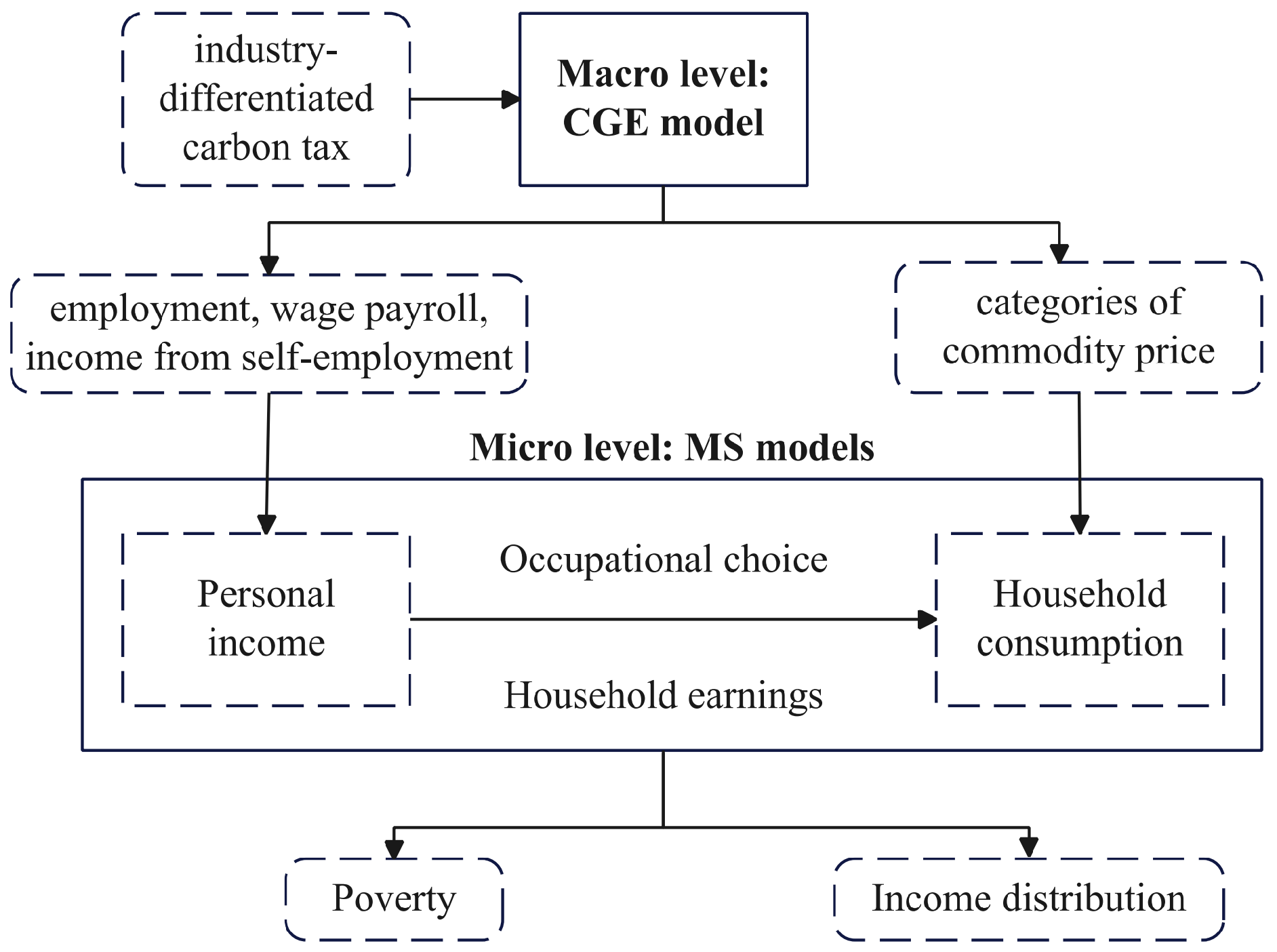
The integration of a macro CGE model with microsimulation (MS) models allows analysis of micro-level impacts (e.g., income distribution, poverty) from external shocks like fiscal or structural policy adjustments. Specifically, changes in employment, wages, and prices estimated by the CGE model are fed into MS models, which then estimate changes in micro variables such as labor income across education levels and household consumption. This enables analysis of social wealth distribution and calculation of inequality and poverty indices. By constructing Growth Incidence Curves (GIC), this article visually compares simulation results between baseline and other counterfactual scenarios to identify the policy’s social welfare impacts and the types of residents most affected.

To be specific, the study first uses household survey data to estimate econometric models of occupational choice, personal income, household earnings, and consumption patterns. Then, it imports percentage changes (relative to the baseline) of macro variables from the CGE model into MS models. Changes in labor demand and wages determine personal income levels, while variations in consumer prices affect household expenditure and purchase quantities across goods. Finally, it calculates indicators such as poverty incidence, Gini coefficient, and Sen index, to evaluate poverty severity and income inequality. Figure 1 shows the connection between CGE model and MS models.

4.4. Data Sources and Processing

The microsimulation analysis relies on data from the 2018 China Family Panel Studies (CFPS), which cover 14,241 households and 41,123 individuals (including 8454 children) and are consistent with the base year of the CGE model. Since the CFPS does not involve the concept of household head, this study follows existing studies [39,40] and identifies “respondent who is most familiar with household finances” as household head. This paper refers to the widely adopted OECD equivalence scale to adjust for household size [41,42]: a weight of 1 is assigned to each adult, 0.5 to teenagers aged 14–18, and 0.3 to children under 14. Equivalent household income and consumption expenditure are calculated accordingly. In line with China’s Classification of Household Consumption Expenditure (2013), this article categorizes household consumption into eight groups: food, tobacco and alcohol, clothing, residence, household goods and services, transportation and communication, education, culture and entertainment, healthcare, and other goods and services. Definitions of core variables are presented in Appendix A.2 

Table A2. Microscopic simulation variables descriptions.

Variable	Description
urban	Household registration type: urban (=1), rural (=0)
region	Economic regions: east (=1), central (=2), west (=3), northeast (=4)
equiv	Equivalent adult coefficient: adult (=1), adolescent (=0.5), child (=0.3)
gender	Gender: male (=1), female (=0)
age	Age (year)
married	Marital status: married (=1), unmarried (=0)
n_children	Number of children (person)
education	Education level: not attending school (=1), primary school (=2), junior high school (=3), high school (=4), university (=5), graduate school (=6)
skilled	Skill level: skilled (=1), unskilled (=0)
worker	Occupational categories: employed (=1), self-employed (=2), agricultural production (=3), unemployed (=4)
school	Study status: yes (=1), no (=0)
wage	Salary level (CNY)
rev_2	Household income from self-employed work (CNY)
rev_3	Household income from agricultural production (CNY)
hsize	Household size (person)
hh_head	Household head: yes (=1), no (=0)
exp_1∼exp_8	Household expenditure on certain type of consumer goods (CNY)
n_worker2	Number of self-employed workers in the household
n_worker2_0	Number of unskilled workers engaged in self-employed work in the household
n_worker2_1	Number of skilled workers engaged in self-employed work in the household
n_worker3	Number of workers engaged in agricultural production in the household
n_worker3_0	Number of unskilled workers engaged in agricultural production in the household
n_worker3_1	Number of skilled workers engaged in agricultural production in the household

.

5. Results and Discussions

5.1. Impact on Poverty Incidence

Poverty incidence (proportion of population below poverty line) reflects the breadth of poverty. This paper adopts two absolute poverty lines: World Bank’s international standard of USD 1.9 per person per day (in 2011 constant prices) and China’s official absolute poverty line of CNY 2300 per capita annual net income (in 2010 constant prices). Adjusted for exchange rates and price levels, the two absolute poverty lines are converted to CNY 5160 and CNY 2995 per capita per year (in 2018 prices), respectively. This study also defines the relative poverty line as one-third of the average annual per capita income of China’s four major economic regions (eastern, central, western and northeastern), calculated based on 2018 CFPS data.

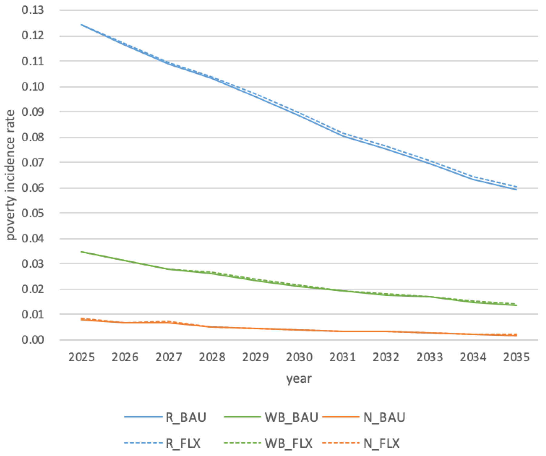
Figure 2 plots poverty incidence trends for relative (R), World Bank (WB), and National (N) poverty lines under BAU and FLX scenarios. As shown in the figure, all poverty indicators decline over time. In the BAU scenario, the relative poverty incidence drops by 52.1% from 0.124 in 2025 to 0.056 in 2035. The international and national absolute poverty rates fall by 60.3% (from 0.035 to 0.014) and 77.4% (from 0.008 to 0.002), respectively. These results demonstrate that poverty alleviation progresses steadily under China’s high-quality development strategy. In addition, relative poverty is significantly higher than absolute, which is consistent with China’s long-term relative poverty challenge.

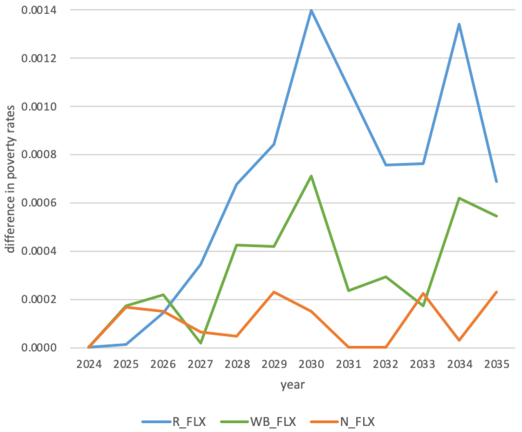
With carbon tax, the decline in poverty incidence is slightly dampened. Taking the FLX scenario as an example, all curves in Figure 3 lie above the zero mark, indicating that a carbon tax raises poverty rates relative to the BAU scenario. Specifically, the poverty gap between the FLX and BAU scenarios widens in the first five years after tax implementation and gradually stabilizes after 2030. Moreover, the adverse impact of a carbon tax on relative poverty is larger than on absolute poverty, but the magnitude stays within 0.14 percentage points, implying that an industry-differentiated carbon tax will not substantially hinder poverty alleviation or cause large-scale re-poverty.

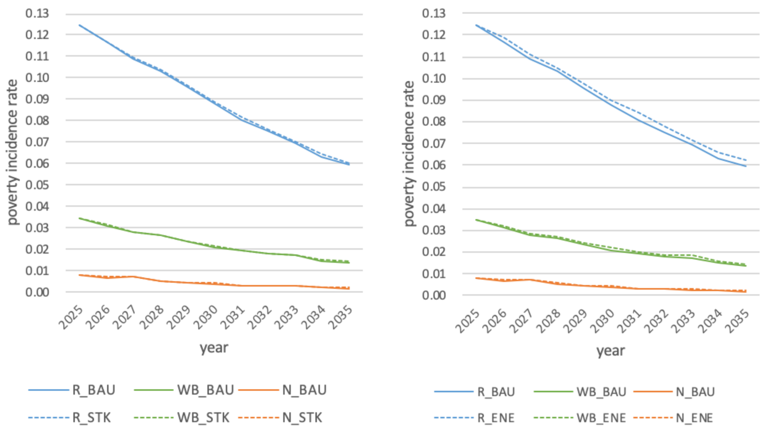
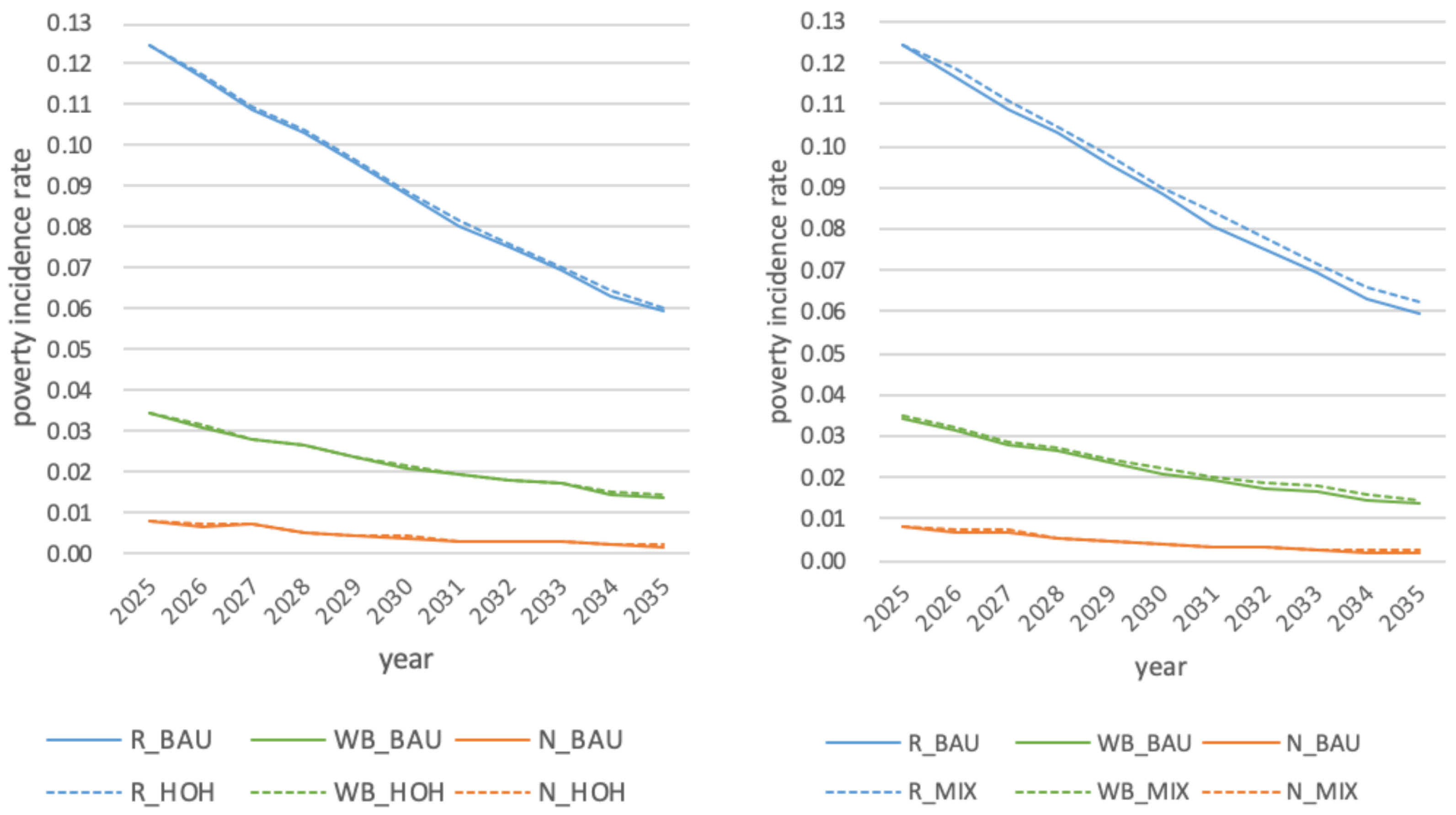
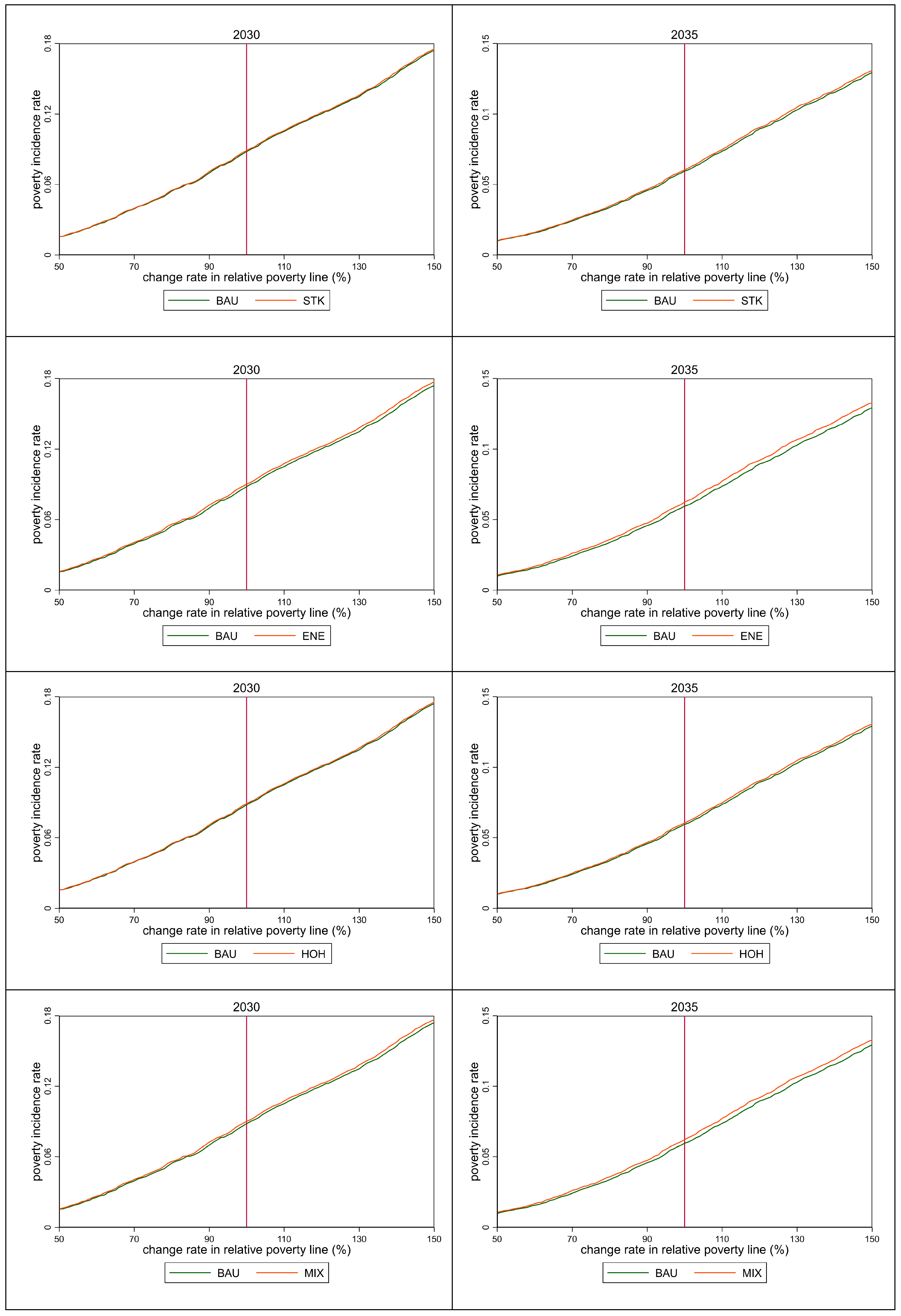
Appendix B Figure A1 shows poverty rates for other counterfactual scenarios. The declining trend is robust, and the tax always slows the decline (i.e., the dashed line lies above the solid line). The difference between the STK and FLX scenarios is negligible (at the ten-thousandth level), meaning that carbon tax rate adjustment frequency has little impact on poverty incidence.

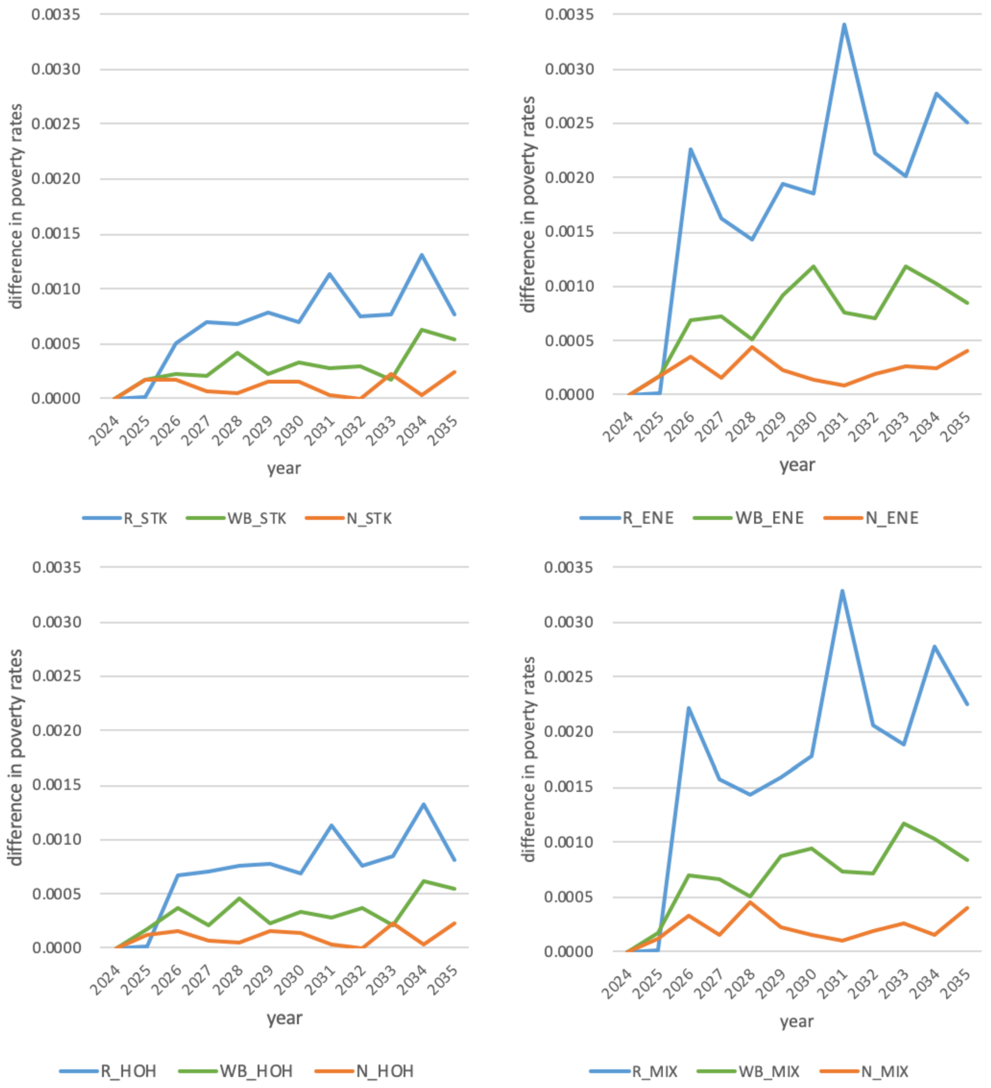
Appendix B Figure A2 further illustrates that revenue recycling cannot fully offset the adverse impact of carbon tax on poverty. However, the degree of deviation from BAU scenario differs. For relative poverty in 2035, ENE, MIX and HOH scenarios yield poverty incidence reductions of 49.8%, 50.1%, and 51.4%, respectively, compared to BAU scenario. Thus, allocating revenues to households alleviates policy shocks on families and reduces public resistance to carbon taxes.

Overall, the negative poverty impact of an industry-differentiated carbon tax is modest. The reason may be that on one hand, producers pass part of the tax burden to consumers via higher prices, so the poor bear some burden, worsening poverty slightly; on the other hand, according to the simulation results from the CGE model, energy-intensive product prices rise significantly, but the poor spend a larger share on necessities like food and clothing rather than energy-intensive goods [43]. Hence the adverse effect is limited, and household-oriented revenue transfers further reduce it.

Notably, China officially eliminated absolute poverty in February 2021, while the model predicts positive poverty incidence. This is because the simulation is based on 2018 data and China accelerated its pace of poverty reduction after 2018. Despite the deviation in absolute values, the downward trend of poverty rates in simulations reliably indicates that carbon taxes will not reverse China’s poverty alleviation progress. This finding remains instructive for the formulation and implementation of carbon taxes.

5.2. Income Distribution Effects

5.2.1. Gini Coefficient

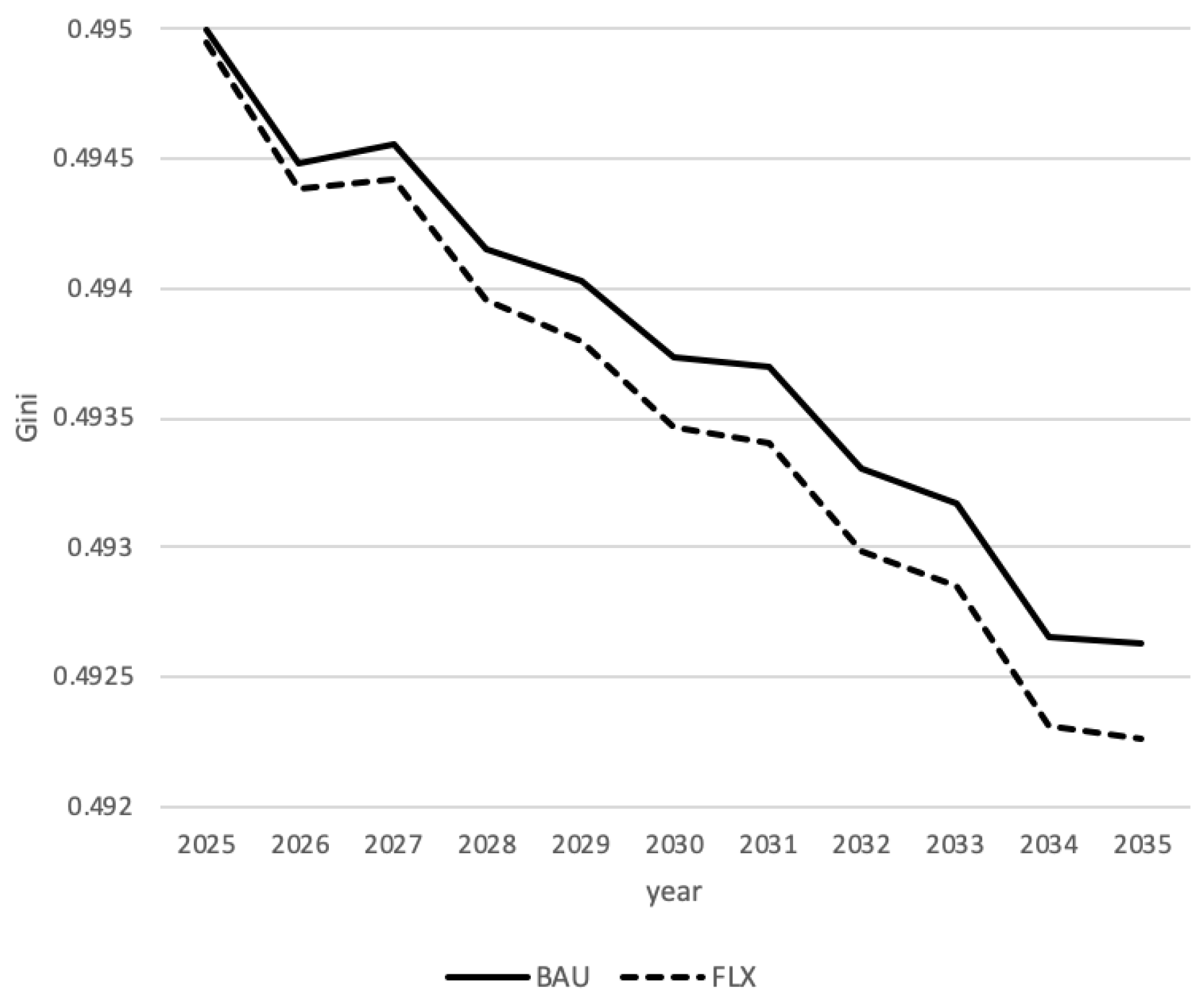
The Gini coefficient measures income dispersion, ranging from 0 (perfect equality) to 1 (perfect inequality). Figure 4 shows China’s Gini coefficient slowly declining. In the BAU scenario, the Gini coefficient falls from 0.4950 in 2025 to 0.4926 in 2035, a reduction of 0.48%. Carbon taxation further narrows the income gap: the Gini coefficient drops by 0.54% in the FLX scenario over the same period. The tax promotes income equality, possibly because increased government revenue allows more public investment, education, healthcare, and transfer payments, which deliver benefits to the public and compress income disparities. While the absolute values of Gini coefficient may differ from reality due to sample representativeness, the trend is informative.

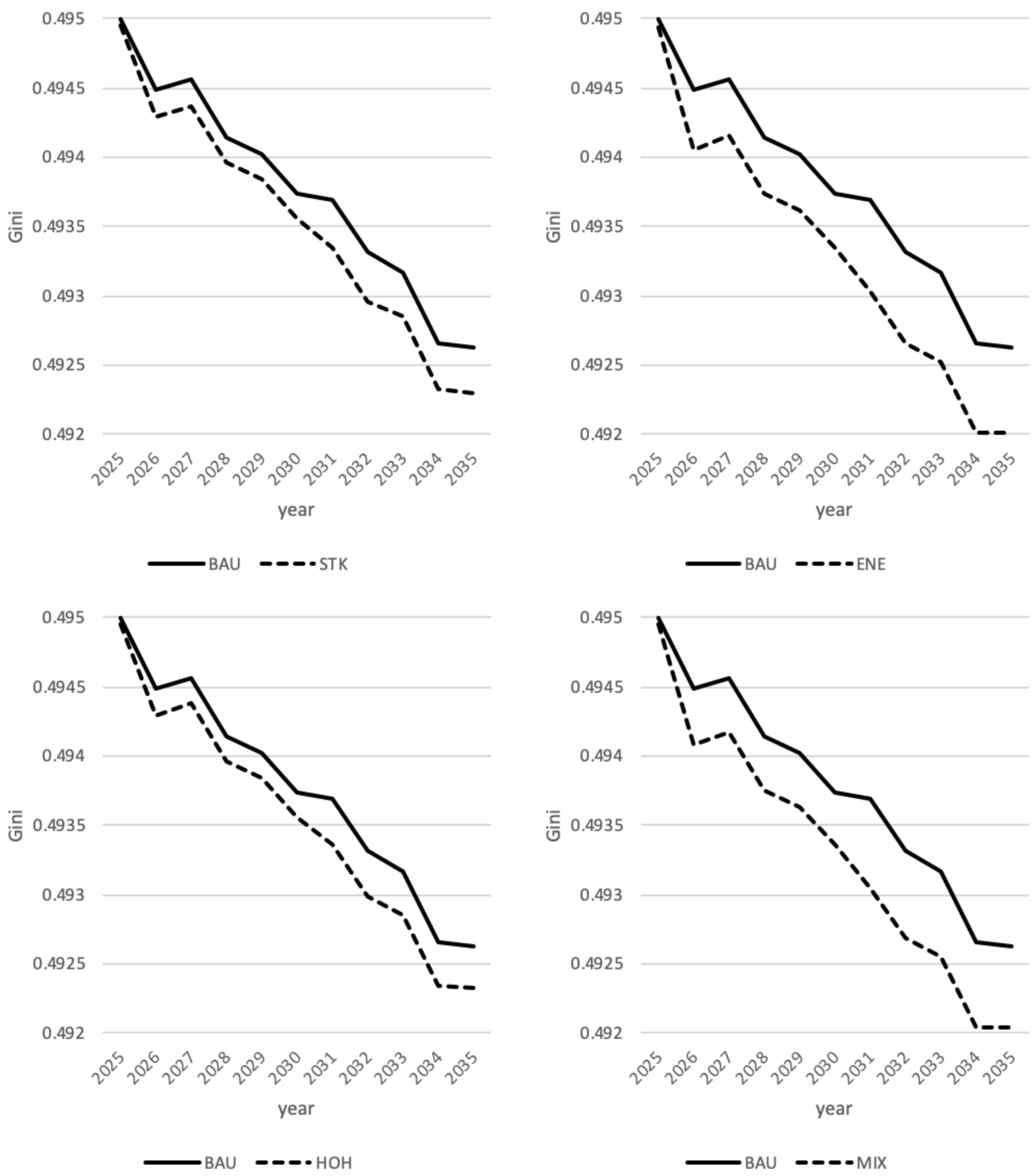
Appendix B Figure A3 presents Gini coefficients under the STK, ENE, HOH and MIX scenarios. As can be seen, the declining trend of the Gini coefficient is robust. The annual difference between the STK and FLX scenarios is minimal, confirming that tax rate adjustment frequency exerts no meaningful influence on income equality. Notably, revenue recycling strategies generate heterogeneous effects on the Gini coefficient: the Gini coefficients decline by 0.531%, 0.588% and 0.591% under the HOH, MIX and ENE scenarios, respectively. In other words, increasing the share of revenues subsidizing the clean power sector further reduces income inequality, which is consistent with the prior literature [4,44,45]. Transferring tax revenue to households is detrimental to narrowing income gap, and the underlying reasons can be explained by the GIC.

5.2.2. Growth Incidence Curve (GIC)

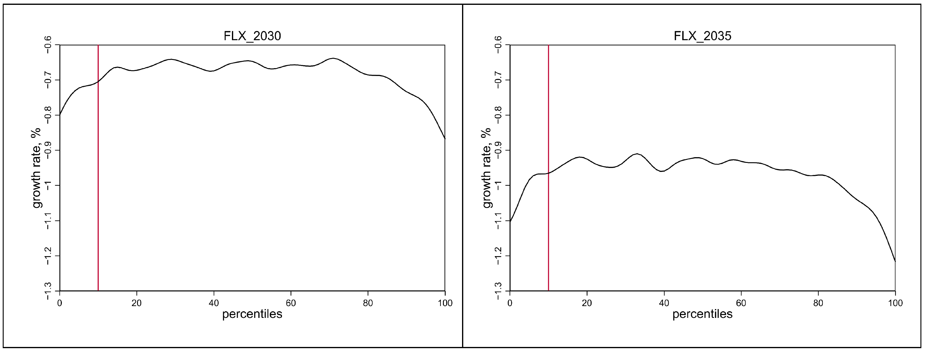
The GIC proposed by Ravallion and Chen [46], depicts changes in income distribution across percentiles. This paper modifies the traditional GIC, normalizing the BAU scenario to zero, with the horizontal axis representing population percentiles ranked by income, and the vertical axis denoting the annualized growth rate of expenditure.

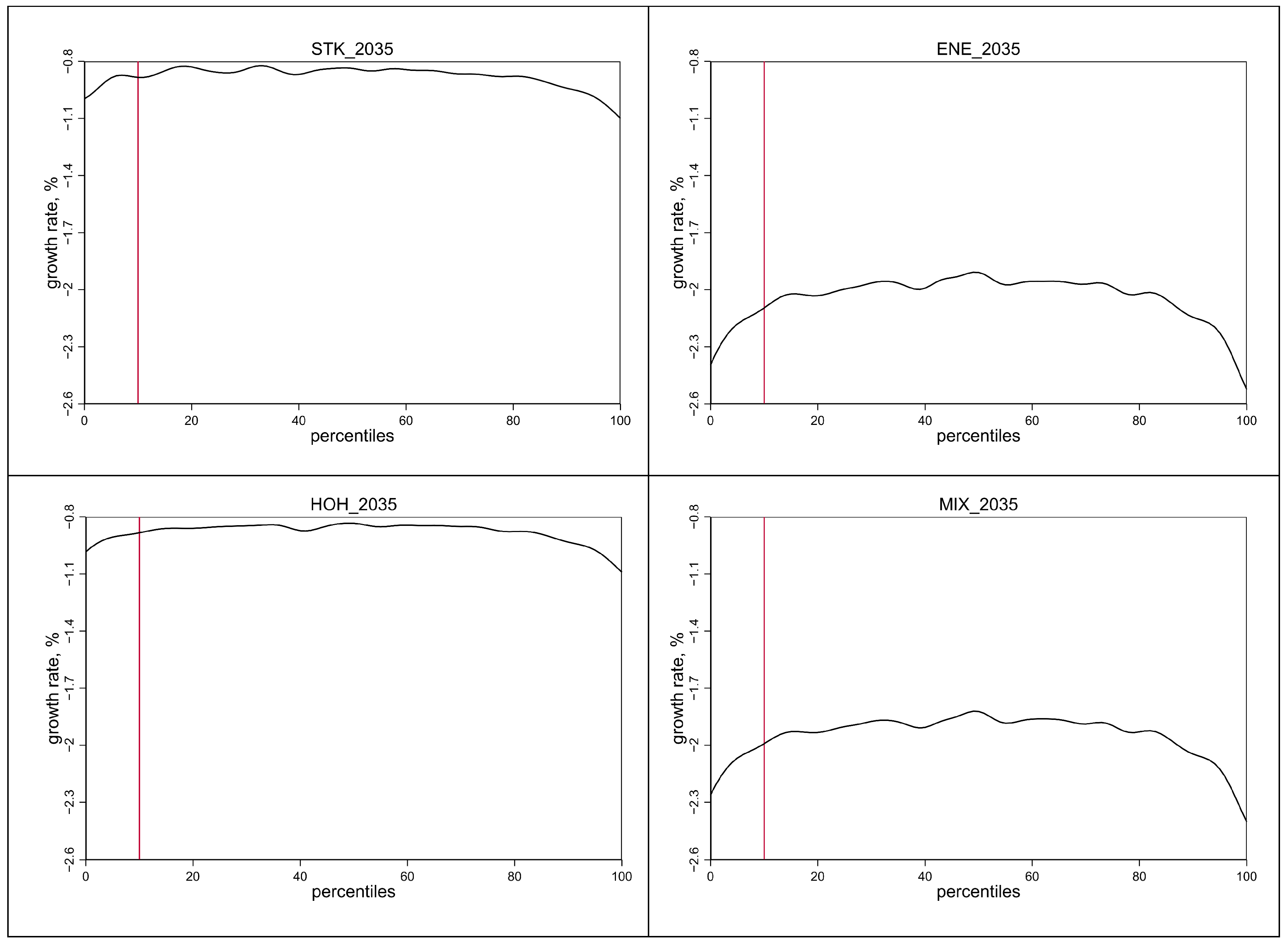
Figure 5 shows GICs under the FLX scenario in 2030 and 2035. The curves are below zero, meaning all income groups reduce expenditure in response to tax-induced price increases, and the adverse impacts intensify over time as carbon tax rates rise. In addition, carbon tax hits the top 20% (80th–100th percentiles) and the bottom 10% (0th–10th percentiles) of the population more severely. In 2035, average consumption decreases by 1.10% for the top 20% and 1.04% for the bottom 10%, while middle-income groups fall by about 0.94%. This evidence verifies the progressive nature of carbon tax in China, as high-income households bear larger burdens than low-income ones. This conclusion differs from prior findings of slightly regressive carbon taxes in China [18], primarily because their multi-regional input–output analysis fails to capture household behavioral responses to price changes and corresponding production adjustments [47]. As highlighted by West and Williams [48], ignoring micro-level behavioral reactions tends to overestimate the poverty and distributional impacts of carbon taxes. Therefore, accounting for supply and demand elasticities and household budget changes can reverse the conclusion.

The negative impact on the bottom 10% partly explains the slight rise in poverty incidence after carbon tax implementation. In absolute terms, consumption reduction by the top 20% is much larger than that of the bottom 10%, so Gini coefficient falls. For low-income households, electricity is the primary energy-consuming product, and regulated electricity prices in China limit carbon tax pass-through [49]. By contrast, high-income households consume a diverse range of energy-intensive goods (e.g., high-emission luxury cars), making them more exposed to carbon tax-induced price hikes.

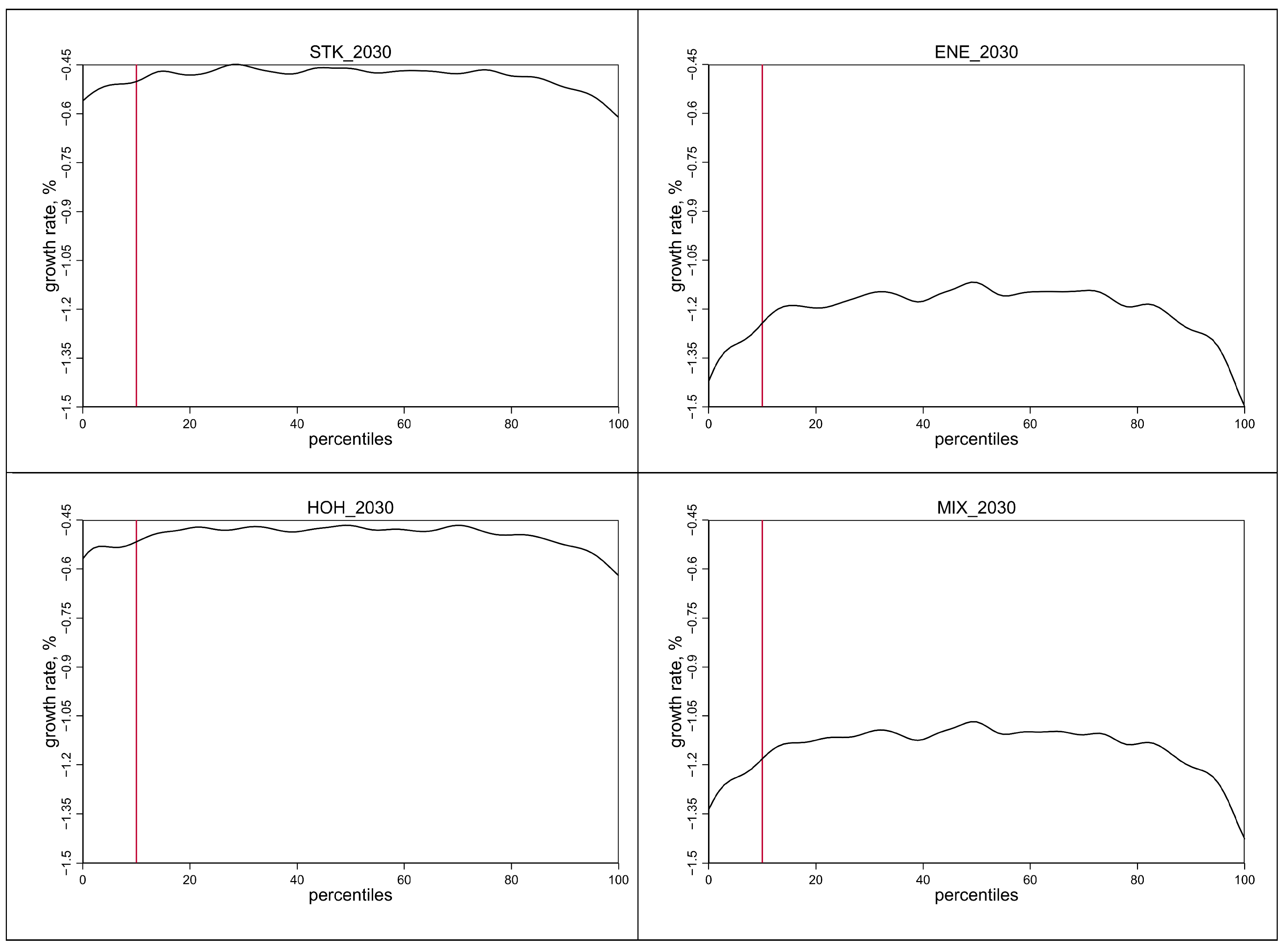
Appendix B Figure A4 and Figure A5, respectively, display GICs for other counterfactual scenarios in 2030 and 2035. In 2030, consumption declines by 0.80% for the poorest group and 0.87% for the richest group in the FLX scenario, compared with 0.56% and 0.61% in the STK scenario. Hence, less frequent tax rate adjustments alleviate consumption shocks. Comparing revenue recycling methods, for middle-income groups (30th–80th percentiles), average consumption drops by 1.16%, 1.10% and 0.48% under the ENE, MIX and HOH scenarios in 2030, respectively. Consistent with the conclusion from the previous discussion on poverty breadth, although none of the simulated tax rebate measures can eliminate the “side effects” of carbon taxes, increasing household transfer payments effectively cushions consumption shocks. Finally, the more subsidy to clean power sector, the larger absolute contribution from the rich, enhancing income equity further: the average expenditure growth rates of the top and bottom 20% of households are −0.56% and −0.53%, −1.28% and −1.24%, −1.35% and −1.31% under the HOH, MIX and ENE scenarios in 2030, respectively.

A comparison reveals that the trends are consistent in the same scenario across different years, but the decline in annual expenditure growth rates varies. From 2030 to 2035, the growth rates of household expenditure in the STK, ENE, HOH, and MIX scenarios decrease by 0.43%, 0.91%, 0.42%, and 0.87%, respectively. Combined with the analysis presented earlier, it can be observed that as time goes by and tax rates increase, promoting renewable energy slows poverty reduction but generates more equitable income distribution.

5.3. Comprehensive Analysis and Robustness Checks

5.3.1. Sen Index

Different revenue recycling strategies create a trade-off between poverty alleviation and income equality: those effective for poverty reduction tend to slow the narrowing of income gaps. To compare the overall performance of recycling strategies, this study calculates the Sen index ($S=H[F+(1-F\left)I\right]$), a comprehensive poverty measurement index integrating poverty incidence (H), poverty gap ratio (F) and the Gini coefficient (I). A higher Sen index indicates lower overall social welfare.

Based on the relative poverty line,

Table 1. Sen index from 2025 to 2035 under BAU and HOH scenarios (%).

Year	H_BAU	F_BAU	I_BAU	S_BAU	H_HOH	F_HOH	I_HOH	S_HOH
2025	12.431	4.076	49.500	6.409	12.433	4.086	49.495	6.410
2026	11.649	3.732	49.448	5.980	11.726	3.772	49.429	6.020
2027	10.908	3.420	49.456	5.583	10.987	3.458	49.438	5.624
2028	10.304	3.131	49.415	5.255	10.391	3.169	49.396	5.299
2029	9.572	2.859	49.402	4.868	9.661	2.894	49.384	4.913
2030	8.813	2.602	49.374	4.467	8.891	2.635	49.356	4.507
2031	8.054	2.374	49.369	4.073	8.183	2.427	49.336	4.138
2032	7.532	2.188	49.331	3.799	7.617	2.239	49.299	3.842
2033	6.959	1.998	49.317	3.503	7.055	2.045	49.285	3.550
2034	6.301	1.820	49.265	3.162	6.450	1.862	49.234	3.236
2035	5.954	1.674	49.263	2.984	6.047	1.714	49.233	3.030

and

Table 2. Sen index from 2025 to 2035 under MIX and ENE scenarios (%).

Year	H_MIX	F_MIX	I_MIX	S_MIX	H_ENE	F_ENE	I_ENE	S_ENE
2025	12.433	4.087	49.495	6.410	12.433	4.089	49.494	6.410
2026	11.900	3.826	49.408	6.110	11.904	3.831	49.406	6.112
2027	11.085	3.510	49.417	5.675	11.092	3.515	49.415	5.678
2028	10.466	3.219	49.376	5.338	10.466	3.222	49.373	5.338
2029	9.752	2.941	49.364	4.959	9.793	2.945	49.362	4.980
2030	9.015	2.679	49.336	4.570	9.023	2.683	49.335	4.574
2031	8.426	2.495	49.305	4.261	8.441	2.501	49.302	4.269
2032	7.766	2.301	49.268	3.917	7.784	2.307	49.265	3.926
2033	7.172	2.104	49.255	3.609	7.188	2.109	49.252	3.617
2034	6.615	1.917	49.205	3.319	6.615	1.921	49.201	3.319
2035	6.209	1.765	49.204	3.111	6.239	1.770	49.201	3.126

, respectively, report the Sen index (S) and its components across scenarios from 2025 to 2035. Compared with the BAU scenario, all carbon tax scenarios witness higher poverty incidence and poverty gap ratios. This may be because low-income groups such as retirees and the unemployed cannot directly benefit from tax credits used to simulate household transfers [50].

Meanwhile, carbon taxes reduce the Gini coefficient. As the revenue share for household transfers decreases (HOH > MIX > ENE), both the poverty incidence and the poverty gap ratio rise while the Gini coefficient falls, leading to a higher Sen index. This indicates that although subsidizing the clean power sector further narrows income gaps, it fails to offset the deterioration of poverty outcomes, resulting in lower social welfare. The macro-level CGE simulation results reveal that (see details in [35]), in the ENE scenario, the share of various renewable energy sources is consistently lower than in the other counterfactual scenarios, whereas the share of fossil energy is correspondingly higher. That is, tax subsidies targeting the clean power generation industry paradoxically reduce the energy share of these sectors. This finding suggests that caution is warranted in the design of carbon taxes and their policy combinations; inappropriate revenue recycling measures can induce resource misallocation, thereby causing policy outcomes to deviate from original intentions. Therefore, to balance multiple policy objectives, HOH scenario is preferable to mitigate the drag on poverty alleviation.

5.3.2. Robustness Analysis

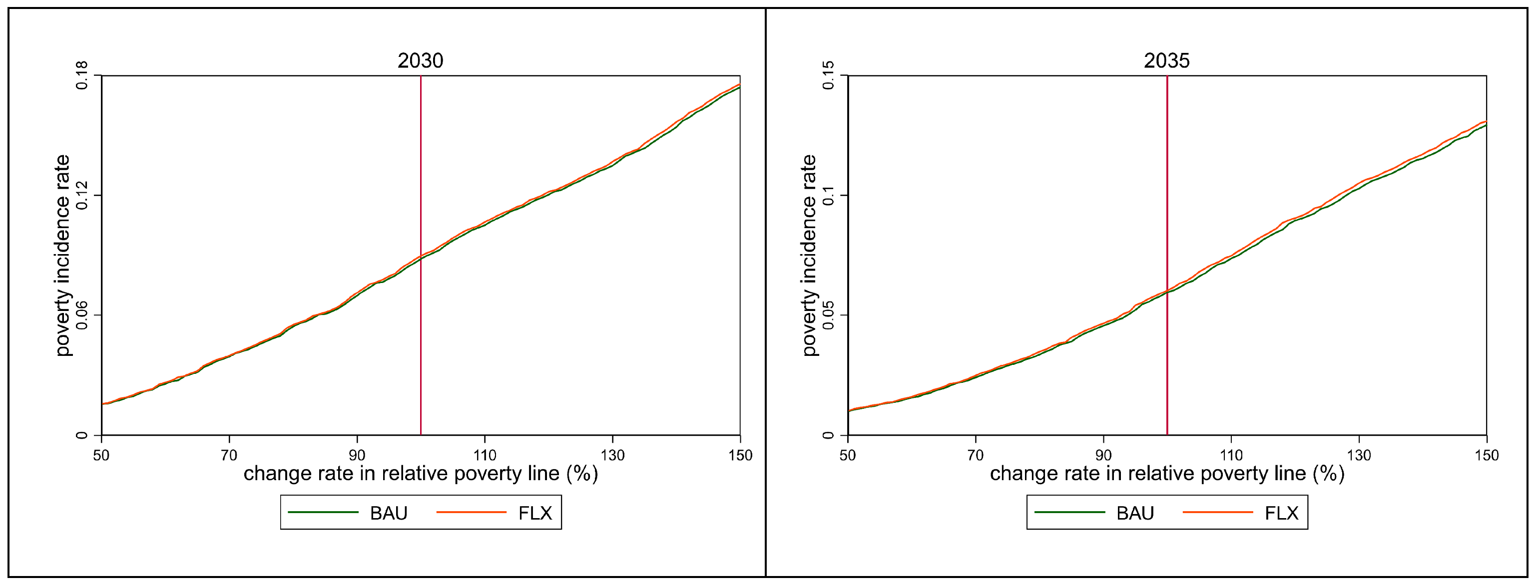
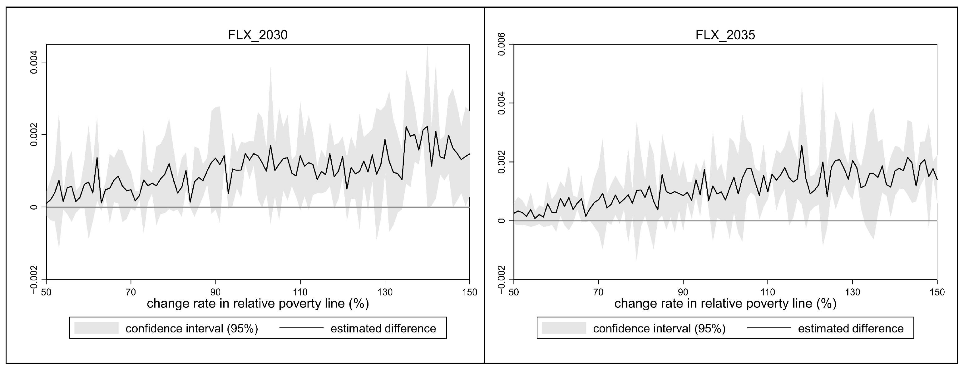
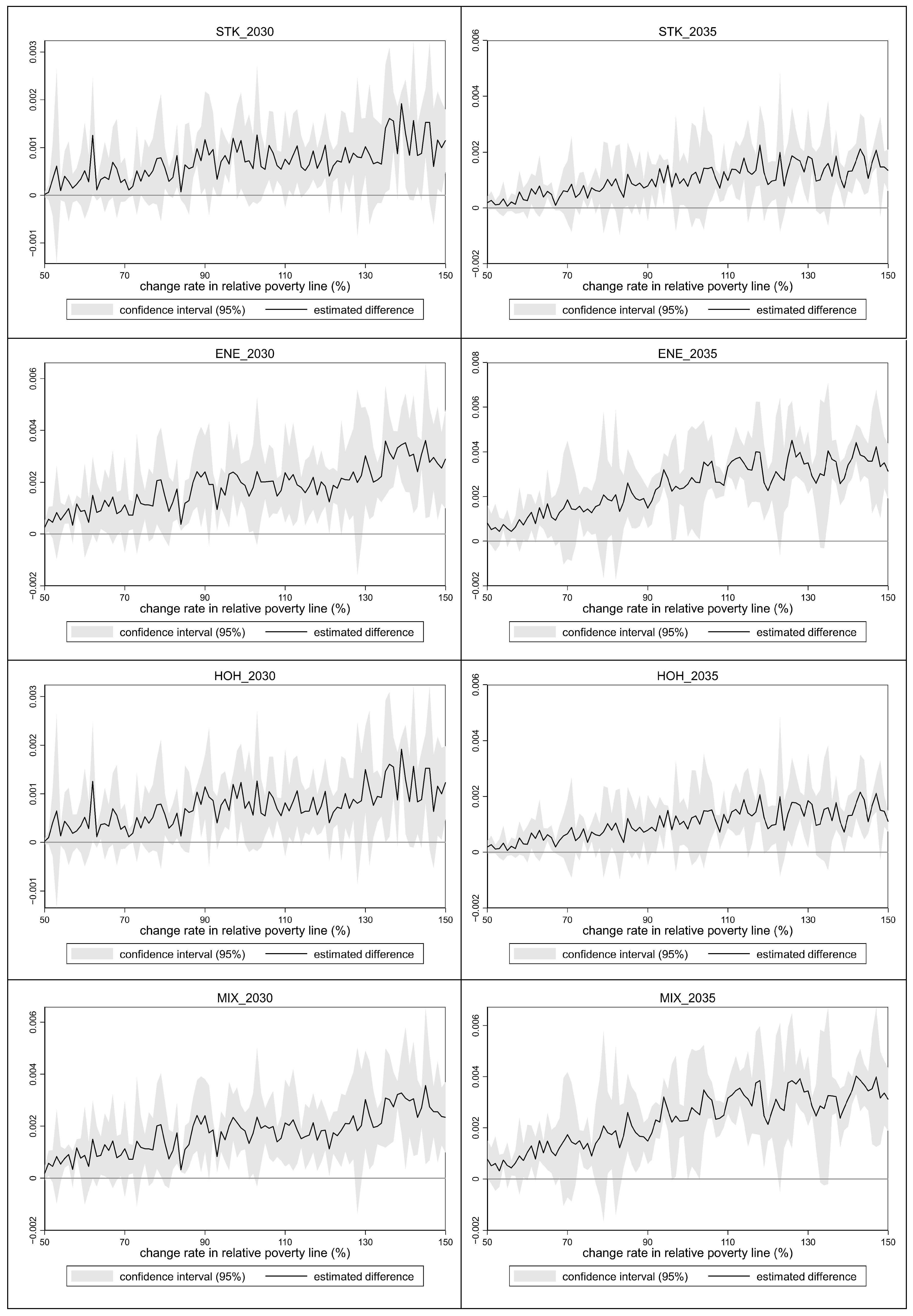
This paper tests the robustness of conclusions by adjusting the relative poverty line within a ±50% fluctuation range. Figure 6 shows that poverty incidence under the FLX scenario remains consistently higher than the BAU scenario in 2030 and 2035 across all adjusted poverty lines. Figure 7 verifies that the poverty gap between the two scenarios is statistically significant. Robustness tests for other scenarios yield consistent results (see Appendix B Figure A6 and Figure A7 for details), confirming the reliability of core findings.

6. Conclusions

The direction and degree of the impacts of carbon tax on income distribution and poverty issues are important factors determining whether it is politically accepted by the public. Using the CGE-MS method, this paper analyzes the micro-level effects of an industry-differentiated carbon tax in China from 2025 to 2035. The main conclusions are summarized as follows:

Firstly, carbon tax slightly slows the pace of poverty reduction, but only modestly. Compared to the BAU scenario, poverty rates rise but do not reverse the declining trend. For the FLX scenario, relative poverty incidence falls 51.5% over the simulation period. Across all counterfactuals, the maximum increase in poverty incidence is within 0.35 percentage points. China need not abandon carbon tax implementation over concerns about rising poverty.

Secondly, carbon tax promotes income equality. The Gini coefficient declines further in all carbon tax scenarios, and the difference from the BAU scenario is −0.03, −0.06, and −0.06 in 2035 under the HOH, MIX and ENE scenarios, respectively. The GIC results confirm the progressive nature of carbon tax in China, which imposes heavier burdens on high-income groups.

Thirdly, revenue recycling effectively mitigates the shock to households. In 2030, the HOH scenario reduces average expenditure by only 0.48%, compared to 1.16% under the ENE scenario. From the calculation results of the Sen index, it can be seen that increasing the transfer payment ratio of carbon tax revenue to the resident sector will alleviate the overall poverty level. In 2035, the comprehensive poverty level under the ENE, MIX, and HOH scenarios is 4.76%, 4.26%, and 1.54% higher than the BAU scenario, respectively, showing a gradually decreasing trend.

These findings have sparked some policy considerations:

• Implement carbon tax with dual priorities of decarbonization and equity.

While the emission reduction effects of carbon tax are well recognized, to enhance public acceptance, policymakers should highlight the role of carbon tax in promoting income equity, and enhance transparency by regularly disclosing the scale, sources, and specific uses of tax revenues. Furthermore, revenue recycling is necessary but requires careful design. The study finds that carbon tax already stimulates demand for clean energy; additional subsidies to the clean electricity sector may lead to overheating and reduced resource allocation efficiency [51]. Hence, when determining subsidized sectors and levels, policymakers should comprehensively assess the behavioral responses of other firms and households to avoid counterproductive outcomes.

• Establish a household welfare-oriented carbon tax revenue recycling mechanism.

To ensure equitable distribution of abatement costs, a dedicated carbon tax welfare fund should be set up to allocate most carbon tax revenues to residents via targeted cash transfers, energy subsidies and universal carbon dividends, with priority given to low-income and energy-vulnerable households. On the one hand, differentiated subsidy standards should be implemented based on household size and income level, and targeted energy consumption vouchers should be issued to identified low-income families on a monthly basis or directly deducted from rigid expenditures such as electricity and heating bills to ensure that their basic energy needs are not affected. On the other hand, additional energy assistance programs should be launched for extremely vulnerable households with a disproportionately high proportion of energy expenditure in their income, accompanied by measures such as special electricity or heat price subsidies for northern heating areas and subsidies for rural clean stove replacement.

• Build a long-term anti-poverty and dynamic adjustment mechanism paired with carbon tax.

Although the overall poverty impacts of carbon tax are modest, a national monitoring system should be established to track key indicators such as poverty incidence and energy expenditure ratios, with a particular focus on vulnerable regions and groups. Automatic adjustment mechanisms should be designed to launch temporary enhanced subsidies or tax rate revisions when monitoring data reveal disproportionate shocks to disadvantaged groups, so as to manage social risks in a proactive and institutionalized manner.

Due to the difficulty of monetizing the additional environmental benefits generated by carbon tax, and the considerable uncertainty surrounding the valuation of emission reduction co-benefits, this paper does not assess the policy’s environmental dividends for micro-agents. Previous studies have indicated that low-income households or workers tend to be more vulnerable to pollutant exposure and possess weaker capacity to withstand pollution-related harm; consequently, they are likely to benefit the most from improvements in environmental quality. If the “indirect environmental benefits” of carbon tax (such as the reduction of extreme weather and air pollution) are taken into account, it may offset its slight adverse impact on the pace of poverty alleviation among disadvantaged groups.