Enabling Sustainable Food Supply Chain Design Through Life Cycle Assessment and Network Optimization: A Plant-Based Protein Case Study in the Mexican Cold Chain

Abstract

This study presents an integrated approach for sustainable food supply chain design by evaluating how sourcing geography and logistics network structure influence Global Warming Potential (GWP) in a multi-echelon Mexican cold chain integrating Life Cycle Assessment (LCA) and Linear Programming (LP) network optimization. Three soy products are evaluated: edamame from China, tofu from the U.S., and textured vegetable protein (TVP) modeled as a soy-based alternative. Results are calculated using a cradle-to-retailer system boundary, normalized to 100 g of delivered protein. Four network configurations are evaluated, varying sourcing geography, port selection, and warehouse allocation. Distribution-stage emissions are minimized through LP optimization, while upstream emissions are incorporated as exogenous LCA parameters. Sourcing geography, distribution-network design, and protein density significantly affect GWP per functional unit, with domestic sourcing yielding the lowest impacts for all products and network configurations. Tofu under the baseline configuration exhibits the highest GWP (1.2236 kg CO₂e/100 g protein), whereas TVP with domestic sourcing exhibits the lowest (0.1146 kg CO₂e/100 g protein), representing a 90.64% difference. The integrated approach provides a decision-support framework for lower-emission sourcing and distribution in emerging-economy food supply chains.

1. Introduction

The decarbonization of global food systems has become a central priority within climate mitigation strategies. Food systems account for approximately one-third of global anthropogenic greenhouse gas emissions (GHG), including emissions from agricultural production, processing, transportation, and retail distribution [1]. Transport-related emissions constitute a substantial share of this impact, with freight mode selection and temperature-controlled logistics significantly influencing carbon intensity [2]. Freight emissions are strongly mode-dependent, with heavy-duty road transport exhibiting significantly higher carbon intensity per tonne-kilometer compared with maritime or rail alternatives [3,4]. These findings highlight the importance of analyzing distribution-stage emissions, particularly in geographically extensive markets.

This issue is particularly relevant in Mexico, where road freight accounts for more than 55% of domestic cargo movement [5]. Road freight has consistently been identified as one of the most carbon-intensive freight modes due to diesel combustion and energy intensity [4]. The country’s geographic extent and reliance on road transport frequently require long-distance freight movements between international gateways and inland consumption centers [6]. Under temperature-controlled conditions, these distances further increase energy requirements and associated emissions, while congestion, road conditions, and freight disruptions can additionally affect transport efficiency [6,7].

Recent food cold chain research identifies sustainability, resilience, and digitalization as central post-pandemic priorities, underscoring the need for integrated environmental–operational approaches [8]. Dietary transitions toward plant-based proteins also offer substantial potential for reducing food-system impacts, with plant-based protein sources generally exhibiting lower cradle-to-gate emissions than ruminant-based systems [9]. Soy-derived products, in particular, demonstrate favorable protein yield per hectare and comparatively low agricultural emission intensity [10]. However, these upstream advantages may be altered by distribution and cold-chain requirements [11], as refrigerated transport and storage require additional energy for temperature control [12]. Moreover, because soy-derived products differ substantially in protein concentration, comparisons based solely on product mass may obscure differences in the amount of protein ultimately delivered. Protein-based functional units can therefore provide a more appropriate basis for comparing the environmental performance of alternative protein products [13]. These characteristics make soy-derived products particularly relevant for evaluating how sourcing geography and cold-chain configuration influence life-cycle emissions.

Life Cycle Assessment (LCA), governed by ISO 14040/14044 standards, provides a structured framework for quantifying environmental burdens across product life cycles [14,15]. Recent research increasingly integrates LCA with supply-chain optimization [16], including multi-objective approaches incorporating environmental and economic objectives, uncertainty, food loss, and product quality [17,18]. Dynamic LCA approaches further account for temporal variability and uncertainty in environmental assessment [19]. Beyond LCA-specific applications, recent numerical studies of transportation systems have evaluated system performance under context-specific operating conditions using validated numerical models [20,21]. Within this broader methodological landscape, the present study focuses specifically on environmental optimization, integrating geographically differentiated life-cycle inventories with a deterministic LP model to evaluate how sourcing geography and distribution-network configuration affect GWP in a multi-echelon Mexican food supply chain.

Mexico combines domestic soybean production with substantial dependence on imports [22,23], creating a relevant context for evaluating sourcing geography. Recent soybean LCA research demonstrates substantial geographical variability in environmental impacts across production systems and regions [24,25], reinforcing the importance of geographically differentiated inventories.

Accordingly, this study addresses the following research questions:

(Q1): How does sourcing geography influence cradle-to-retailer Global Warming Potential (GWP) in soy-derived protein supply chains operating within the Mexican cold chain?

(Q2): How do alternative distribution-network structures affect total GWP under identical demand conditions?

To address these questions, the study integrates attributional LCA with LP network optimization to compare alternative sourcing and distribution configurations for three soy-derived products within a multi-echelon Mexican food supply chain. The analysis contributes a geographically differentiated framework for jointly evaluating sourcing-dependent and network-dependent environmental burdens.

2. Materials and Methods

2.1. Goal and Scope Definition

2.1.1. Goal of the Study

The goal of this study is to evaluate how sourcing geography and distribution-network structure jointly influence the environmental performance of soy-based protein supply chains within a multi-echelon Mexican food distribution system. The study integrates attributional Life Cycle Assessment (LCA) with a Linear Programming (LP) network optimization model to quantify cradle-to-retailer Global Warming Potential (GWP) across three soy products and four sourcing and distribution configurations.

The intended application is to support strategic sourcing and logistics decision-making by distinguishing sourcing-dependent upstream impacts from distribution-stage impacts associated with alternative network structures. Facility locations remain fixed across scenarios, while feasible routing configurations vary; consequently, the optimization model evaluates flow allocation and routing rather than facility-location decisions. The study is comparative and does not seek to make absolute environmental claims outside the defined system boundary.

2.1.2. Type of LCA

This research employs an attributional Life Cycle Assessment (ALCA) approach, conducted in accordance with the ISO 14040 and ISO 14044 standards for environmental management and LCA methodology [14,15]. ALCA quantifies the average environmental burdens associated with the production and distribution of a product within a defined system boundary. An attributional approach is appropriate for this study because the objective is to compare sourcing configurations under fixed demand and infrastructure conditions, rather than to estimate economy-wide market responses —which are typically addressed through consequential LCA modeling [26].

2.1.3. Functional Unit

The primary functional unit (FU) of this study is defined as: 100 g of delivered protein at the retailer gate. Normalization per unit of protein enables nutritionally equivalent environmental comparisons among products with substantially different protein concentrations and moisture contents [10,13].

The use of protein-based functional units has been increasingly recommended in food LCAs to improve cross-product comparability [13]. For transparency and logistical interpretation, intermediate results are additionally reported per kilogram of each respective product transported. This mass-based metric allows the isolation of distribution-stage performance independent of nutritional density but does not constitute a separate functional unit under ISO 14044 [15].

2.1.4. System Boundary

The assessment includes the following life cycle stages:

• Agricultural production of soybeans;
• Industrial processing;
• International transport to Mexican entry points (where applicable);
• Domestic refrigerated or dry distribution across a multi-echelon logistics network.

The boundary excludes retail operational energy consumption, consumer transport and product preparation, and end-of-life and waste management. These exclusions are consistent with the study objective of isolating upstream production and distribution-stage emissions in accordance with ISO 14044 system boundary principles; life cycle stages may be excluded when they fall outside the goal and scope definition [15].

Agricultural production and industrial processing emissions are incorporated as geographically differentiated exogenous LCA parameters, reflecting the conditions applicable to each configuration. International transport emissions are calculated according to the applicable sourcing route, transport mode, and temperature-control condition. In contrast, domestic transport and storage emissions across infrastructure nodes are endogenously determined through the optimization model, allowing environmental impacts to respond dynamically to routing decisions and network flow configurations [9,11,16].

2.1.5. Geographic and Temporal Scope

The geographic scope of the study is Mexico, with international upstream production occurring in:

• Fujian Province, China (Edamame: S1, S2, S3) (TVP: S1, S2, S3);
• California, United States (Tofu: S1, S2, S3);
• Campeche, Chiapas, and Tamaulipas, Mexico (Edamame: S4) (Tofu: S4) (TVP: S4).

Domestic distribution flows represent a multi-echelon network connecting national entry points, transshipment nodes, distribution centers, regional warehouses, and retailer nodes located in seventeen locations across Mexico. The temporal scope represents contemporary supply-chain conditions using the most recent geographically relevant agricultural, processing, energy, and freight inventory data available for the modeled sourcing regions.

2.1.6. Impact Category

The study focuses exclusively on Global Warming Potential over a 100-year time horizon (GWP100), expressed as kg CO₂e, using the characterization factors recommended in the IPCC Fifth Assessment Report (AR5) [3]. This selection is justified because climate mitigation constitutes the primary objective of this research, and GWP100 remains the most widely reported and policy-relevant impact indicator in food system sustainability assessments. The exclusive focus on a single midpoint climate indicator aligns with established comparative food LCA practice where GWP100 serves as the primary decision-relevant metric [3,9]. Other environmental categories (e.g., eutrophication, water consumption, land use) are beyond the scope of this analysis.

2.2. Case Study and Logistics Network

The distribution system analyzed in this study represents a multi-echelon cold chain network reflective of a national food service distribution structure operating across major Mexican metropolitan regions. The baseline scenario (S1) models the current empirical logistics of the firm, characterized by its observed distribution flows and facility utilization patterns.

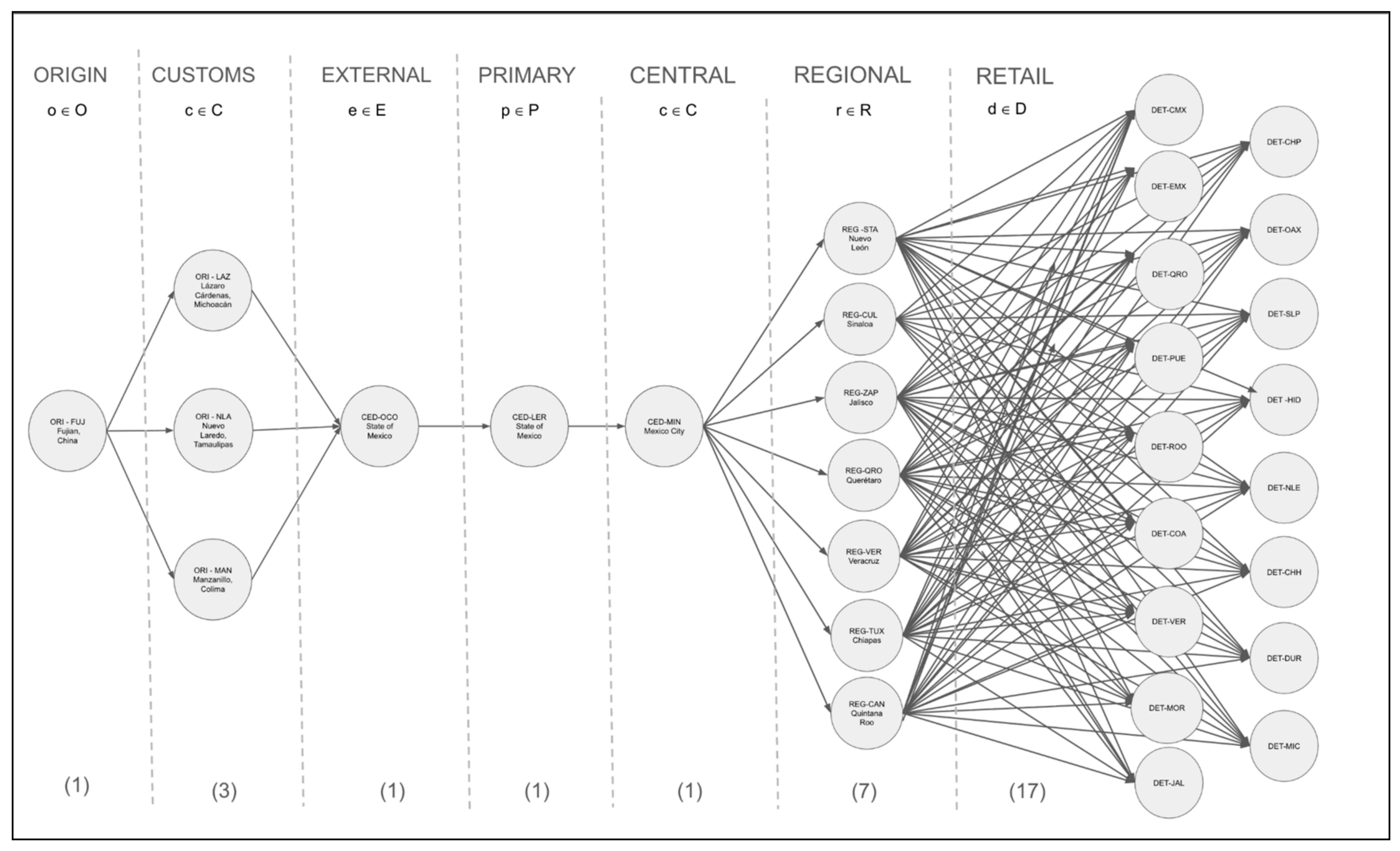
The system consists of seven hierarchical echelons (S1):

• Tier 1—Origin Nodes:

- Edamame Sourcing (S1, S2, S3): Fujian, China.

- Tofu Sourcing (S1, S2, S3): California, USA.

- TVP Sourcing (S1, S2, S3): Fujian, China.

- Domestic Sourcing (S4): For all products: Campeche, Chiapas, and Tamaulipas, Mexico.

• Tier 2—Customs and Ports of Entry:

- (S1): All international products are routed through to Nuevo Laredo, Tamaulipas.

- (S2–S3): The model selects the optimal gateway among Lázaro Cárdenas or Tijuana based on the emission-minimizing path to the central nodes.

• Tier 3—External Storage:

Due to initial consolidation requirements, imports are first received at an external warehouse in the State of Mexico.

• Tier 4—Primary Storage Facility:

Products are transferred to the company’s main storage also in the State of Mexico, which serves as the primary inventory reserve with a capacity five times larger (5:1 ratio) than the central sorting hub.

• Tier 5—Central Distribution Center:

Products move from the State of Mexico to Mexico City central hub. This distribution center functions as the sorting center for regional network dispatch.

• Tier 6—Regional Warehouses:

The company operates a network of regional warehouses that support product distribution across Mexico. In the baseline scenario (S1), flows through regional facilities reflect the firm’s observed logistics practices. For the optimized scenarios (S2–S4), a network design constraint was introduced whereby destinations located more than 100 km from the central hub are supplied through regional warehouses, enabling the evaluation of alternative distribution structures and their environmental performance.

• Tier 7—Retail Demand Nodes:

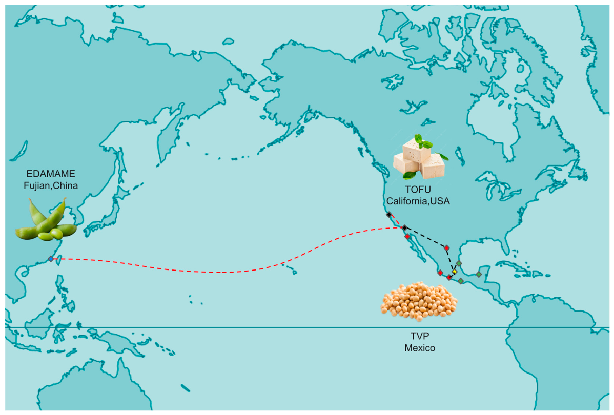
Final delivery to 17 urban retailers across the country. Aggregated nodes representing total periodic demand (3-day inventory cycle) in major metropolitan regions. Figure 1 illustrates the superstructure of the baseline distribution network used in this study for the imported edamame scenario (S1).

Figure 2 illustrates S1 for edamame and tofu: both products are routed through Nuevo Laredo, following the mandatory external–primary–central corridor. In the optimized scenarios (S2–S3), the model is granted the flexibility to endogenously select among all available maritime ports (e.g., Manzanillo, Lázaro Cárdenas and Tijuana) and warehouse nodes to identify the emission-minimizing path, including direct regional flows. In S4 for TVP, domestic sourcing is modeled from the primary soybean-producing regions in Campeche, Chiapas, and Tamaulipas.

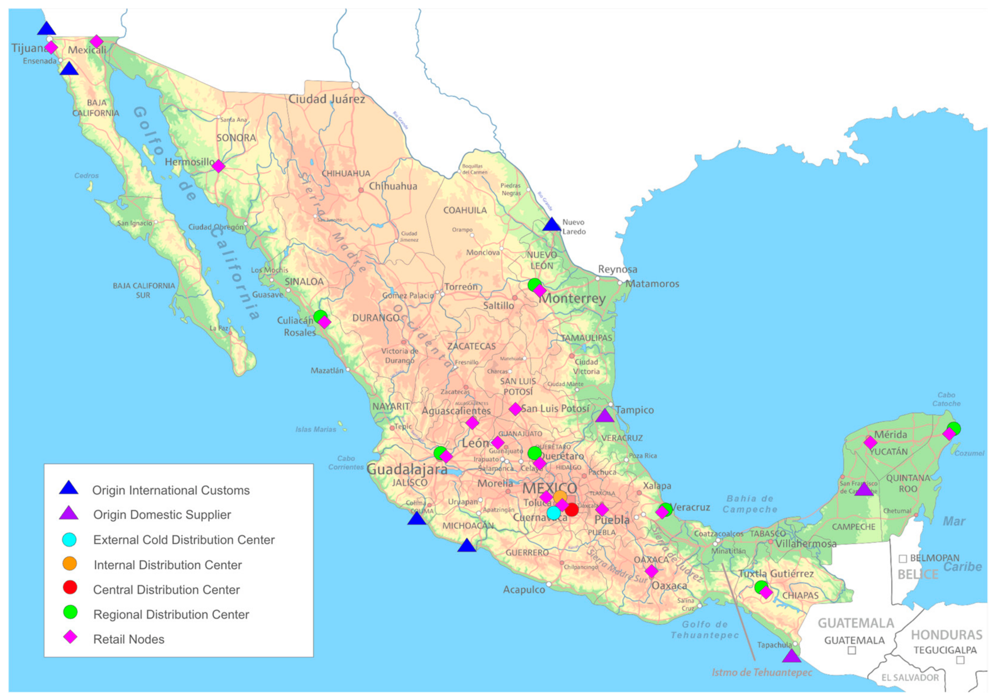
Each retail node represents the total deterministic demand across all stores located within the corresponding metropolitan region. Retail demand is expressed in kilograms of product per 3-day cycle and is treated as identical across sourcing scenarios. All retail demand must be fully satisfied within the optimization model. Figure 3 shows the geographic distribution of sourcing, entry, distribution, regional, and retail nodes across the domestic network.

2.3. Life Cycle Inventory (LCI)

2.3.1. Data Sources and Emission Factors

The life cycle inventory (LCI) phase involves the collection and estimation of all data required to quantify greenhouse gas emissions associated with the comparative plant-based protein supply chains assessed in this study, consistent with ISO 14040/14044 standards [14,15]. Life-cycle inventory data and emission factors were obtained from peer-reviewed literature, governmental and technical sources, and case-study operational data. Sources were selected according to geographical and technological relevance to the modeled agricultural, processing, transportation, and storage stages. This approach aligns with precedent in agricultural LCA research, where inventory data are constructed using distance-based transport modeling, process-specific emission intensities, and product-specific conversion factors [11,27,28,29]. Emission factors were expressed in units appropriate to each life-cycle stage and integrated on a per-kilogram-of-product basis before normalization to the primary functional unit of 100 g of delivered protein.

2.3.2. Upstream Emission Factors

(a) Agricultural emission factors were differentiated by soybean sourcing origin. Values of 0.25 and 0.56 kg CO₂e/kg soybean were adopted for China and the United States based on Ning et al. [30] and Romeiko et al. [31], respectively. For Mexico, no comparable national or state-level soybean LCA inventory was identified; therefore, agricultural GWP was reconstructed for southern Tamaulipas using regional foreground data from FIRA [32] following an inventory-based approach consistent with Pereira et al. [33], who developed state-level agricultural inventories to estimate life-cycle emissions from soybean and other crops. In the present study, the agricultural GWP for southern Tamaulipas was calculated from individual foreground activity data and source-specific emission factors rather than adopted from an aggregate soybean GWP reported in the literature. The reconstruction incorporated agricultural machinery fuel consumption [34], Mexican diesel combustion factors [35], upstream diesel emissions [36], IPCC crop-residue and soil N₂O parameters [37], upstream seed [33], and MAP fertilizer emissions [38]. All activity data, emission factors, and calculations are reported in

Table 1. Parameters and emission factors for soybean LCA in southern Tamaulipas.

Component	Parameters	Values	Units
Production	Soybean yield	1550	kg soybean/ha
Seed	Application; production emission factor	50; 0.43	kg/ha; kg CO2e/kg seed
MAP fertilizer	Application; nitrogen content; production emission factor	90; 0.11; 0.52	kg/ha; kg N/kg MAP; kg CO2e/kg MAP
Field operations	Ploughing; harrowing; ridging; mechanical sowing	1 × 14.3; 2 × 8.0; 1 × 7.0; 1 × 8.0	passes × L/ha/pass
Field operations	Fertilizer application; cultivation; crop-spraying; harvesting	2 × 3.0; 2 × 7.0; 2 × 3.0; 1 × 35.0	passes × L/ha/pass
Diesel	Direct combustion emission factor; net calorific value; well-to-tank emission factor	74,100; 35.95; 18.9	kg CO2/TJ; MJ/L; g CO2e/MJ
Crop residues	Soybean dry-matter fraction; aboveground residue/yield ratio; root-to-shoot ratio; residue nitrogen content	0.91; 2.1; 0.19; 0.008	fraction; ratio; ratio; kg N/kg dry matter
Direct N2O	Synthetic nitrogen emission factor; crop-residue emission factor	0.016; 0.006	kg N2O-N/kg N
Indirect N2O	Volatilized nitrogen fraction; volatilization emission factor; leached nitrogen fraction; leaching emission factor	0.08; 0.014; 0.24; 0.011	fraction; kg N2O-N/kg N; fraction; kg N2O-N/kg N
Characterization	Molecular conversion from N2O-N to N2O; N2O global warming potential	44/28; 265	kg N2O/kg N2O-N; kg CO2e/kg N2O

and

Table 2. Agricultural GWP calculation for southern Tamaulipas.

Component	Calculation	Intermediate Result	kg CO2e/kg Soybean
Seed production	(50 × 0.43)/1550	21.500 kg CO2e/ha	0.01387
Fertilizer production	(90 × 0.52)/1550	46.800 kg CO2e/ha	0.03019
Total field diesel	(1 × 14.3) + (2 × 8.0) + (1 × 7.0) + (1 × 8.0) +(2 × 3.0) + (2 × 7.0) + (2 × 3.0) + (1 × 35.0)	106.30 L/ha	—
Diesel—direct combustion	(106.3 × 35.95 × 74,100/106)/1550	283.172 kg CO2e/ha	0.18269
Diesel—upstream production	[106.3 × (35.95 × 18.9/1000)]/1550	72.226 kg CO2e/ha	0.04660
Synthetic fertilizer nitrogen	90 × 0.11	9.900 kg N/ha	—
Crop-residue nitrogen	[(1550 × 0.91 × 2.1) +((1550 × 0.91 + 1550 × 0.91 × 2.1) × 0.19)] × 0.008	30.34268 kg N/ha	—
Direct N2O-N	(9.9 × 0.016) + (30.34268 × 0.006)	0.34046 kg N2O-N/ha	—
Direct soil N2O	[0.34046 × (44/28) × 265]/1550	141.776 kg CO2e/ha	0.09147
N2O-N from volatilization	(9.9 × 0.08) × 0.014	0.011088 kg N2O-N/ha	—
Indirect N2O— volatilization	[0.011088 × (44/28) × 265]/1550	4.617 kg CO2e/ha	0.00298
N2O-N from leaching/runoff	[(9.9 + 30.34268) × 0.24] × 0.011	0.10624 kg N2O-N/ha	—
Indirect N2O— leaching/runoff	[0.10624 × (44/28) × 265]/1550	44.242 kg CO2e/ha	0.02854
Total agricultural GWP	Sum of emission contributions	614.333 kg CO2e/ha	0.39634

.

The resulting agricultural GWP was 0.39634 kg CO₂e/kg soybean, rounded to 0.40 kg CO₂e/kg for implementation across the three Mexican sourcing regions evaluated in S4. Because comparable foreground inventories were unavailable for Chiapas and Campeche, this coefficient was applied consistently to all three domestic sourcing regions rather than introducing differences driven by data availability. This proxy does not imply equivalent agricultural practices or emission intensities occur across the three states.

(b) Industrial Processing: Emissions were geographically differentiated according to the modeled processing location. Processing energy requirements were obtained from industrial or product-specific literature [39,40,41] and combined with national electricity emission factors for the corresponding processing countries [42,43,44]. For frozen edamame, frozen-pea processing was adopted as the closest available industrial processing proxy because its processing sequence—cleaning, selection, blanching, and freezing—most closely represents the processing requirements of frozen edamame among the frozen vegetables evaluated in the source study [41]. For tofu, both electricity and natural-gas requirements were considered [39,45]. TVP processing was represented using the reported electricity requirement for soy-based TVP extrusion [40]. The resulting geographically differentiated processing emission factors are presented in

Table 3. Processing emission factors by product.

Product	Processing Requirement	S1–S3: Location/Emissions	S4: Location/Emissions	Ref.
Frozen edamame	0.139 kWh/kg	China 0.0804 kg CO2e/kg	Mexico 0.0618 kg CO2e/kg	[41,42,43]
Tofu	0.329 kWh/kg electricity; 0.117 m3/kg natural gas	United States 0.3403 kg CO2e/kg	Mexico 0.3713 kg CO2e/kg	[39,42,44,45]
TVP	0.260 kWh/kg	China 0.1502 kg CO2e/kg	Mexico 0.1154 kg CO2e/kg	[40,42,43]

.

2.3.3. Domestic and International Transport Emission Factors

Maritime transport was based on Fitzgerald et al. [46], who reported 0.018 kg CO₂e/t km for temperature-controlled food transport, with approximately 19% of transport energy attributable to refrigeration. This coefficient was applied to frozen edamame, while exclusion of the refrigeration share yielded the non-temperature-controlled coefficient for TVP.

Road transport was based on the Mexico-specific well-to-wheel intensity reported by Serrano-Guevara et al. [47], converted assuming a 25 t payload. Refrigeration was modeled separately from vehicle propulsion following du Plessis et al. [48], consistent with previous cold-chain studies [12,49]. For U.S. road segments, the non-temperature-controlled freight factor was calculated from U.S. EPA medium- and heavy-duty truck emission factors using IPCC AR5 GWP100 characterization factors, while refrigeration was incorporated separately following du Plessis et al. [3,45,48]. The resulting maritime and road emission factors are reported in

Table 4. Domestic and International Transport Emission Factors.

Transport Mode	Condition	Emission Factor	Unit	Source
International maritime transport	No temperature control	0.0000146	kg CO2e/(kg·km)	[46]
International maritime transport	Temperature-controlled	0.0000180	kg CO2e/(kg·km)	[46]
Domestic heavy-duty road transport	No temperature control	0.0000605	kg CO2e/(kg·km)	[47]
Domestic heavy-duty road transport	Temperature-controlled	0.0000650	kg CO2e/(kg·km)	[47,48]
International heavy duty road transport	No temperature control	0.0001284	kg CO2e/(kg·km)	[3,45]
International heavy duty road transport	Temperature-controlled	0.0001329	kg CO2e/(kg·km)	[3,45,48]

.

2.3.4. Storage and Cold Chain Emission Factors

Temperature-controlled storage emissions were reconstructed from case-study operational data and external technical parameters (

Table 5. Parameters used to reconstruct the temperature-controlled storage emission intensity.

ID	Parameter	Value	Unit	Source
S1	Installed PV capacity	600	kWp	Case-study technical assessment
S2	Average solar irradiation	5.8	kWh/m2/day	SENER, Atlas Nacional
S3	Inverter conversion efficiency	0.95	fraction	NOM-001-SEDE-2012, Art. 210-19
S4	Voltage-loss adjustment factor	0.97	fraction	NOM-001-SEDE-2012, Art. 210-19
S5	PV electricity contribution ratio	0.25	ratio	Case-study technical assessment
S6	SEN electricity emission factor	0.444	kg CO2e/kWh	CRE, SEMARNAT
S7	Storage allocation mass-normalization factor	8.333 × 10−8	kg−1	Case-company operational information
S8	External inventory holding range	15–30	days	Case-company operational information
S9	Central inventory holding range	7–15	days	Case-company operational information
S10	Primary/regional inventory holding time	3	days	Case-company operational information

). Photovoltaic electricity generation was estimated using the installed capacity, average solar irradiation from SENER [50], and system-performance parameters from NOM-001-SEDE-2012 [51], following the performance-monitoring framework of IEC 61724-1:2021 [52]. Grid-related emissions were calculated using the national electricity emission factor reported by CRE and SEMARNAT [42]. Commercially sensitive allocation and product-mass data were aggregated into a mass-normalization factor to preserve the calculation procedure without disclosing confidential operational information.

The reconstructed daily temperature-controlled storage coefficient (

Table 6. Reconstruction of the temperature-controlled storage emission intensity and daily storage emission coefficients.

Calculation Component	Parameters	Calculation	Result	Unit
PV performance factor	S3–S4	0.95 × 0.97	0.9215	—
Monthly PV electricity generation	S1, S2; PV performance factor	600 × 5.8 × 0.9215 × 30	96,204.60	kWh/month
Total electricity demand	S5	96,204.60/0.25	384,818.40	kWh/month
SEN-supplied electricity	S5	384,818.40 × (1 − 0.25)	288,613.80	kWh/month
Electricity-related emissions	S6	288,613.80 × 0.444	128,144.53	kg CO2e/month
Monthly storage emission intensity	S7	128,144.53 × 8.333 × 10−8	0.0106787	kg CO2e/kg-month
Daily storage emission coefficient	Monthly storage emission intensity	0.0106787/30	0.00035596	kg CO2e/kg-day

) was applied according to the inventory holding time at each warehousing echelon. External and central storage were modeled using midpoint holding times of 22.5 and 11 days, respectively, based on operational ranges of 15–30 and 7–15 days. Primary and regional warehouses were assigned a 3-day holding time, consistent with the short replenishment cycle reported for these stages. Imported temperature-controlled products were additionally assigned a 3-day port dwell time based on refrigerated-container and terminal evidence [53,54] during which continued electricity supply is required for temperature control [55].

Storage emissions were applied only to the warehousing echelons traversed in each network configuration; therefore, bypassing an upstream facility also avoided its associated holding time and emissions. This treatment reflects the dependence of cold-storage impacts on electricity consumption and inventory duration [12,28]. Non-temperature-controlled tofu and TVP were assigned no cold-storage emissions, while general warehouse electricity use was excluded because product-specific operational data were unavailable.

2.3.5. Protein Content and Functional Basis Data

Protein content values for each product were extracted from nutritional datasets used in food LCAs: USDA [56] for edamame and tofu, and Herrmann et al. [10] for TVP concentration. Protein content was used to normalize final GWP results to the defined functional unit of 100 g of delivered protein [13].

2.3.6. Data Quality, Assumptions, and Limitations

All emission factors were selected based on geographical and technological relevance, recency, and consistency with LCA best practices. Where direct data were unavailable, proxy factors from peer-reviewed or authoritative technical sources with transparent methodologies were used. Geographically differentiated data were prioritized for agricultural production, processing, electricity supply, and transportation wherever available. Where Mexico-specific emission factors were unavailable, proxy values were selected based on technological similarity, production-system comparability, and consistency with ISO 14044 data-quality requirements [15]. Remaining data limitations and proxy assumptions were explicitly documented and applied consistently across comparable scenarios. Although residual regional and operational variability may influence absolute emission magnitudes, this approach supports transparent comparative evaluation of sourcing and distribution configurations.

2.4. Optimization Model

2.4.1. Formulation

To evaluate emission-minimizing distribution strategies across sourcing scenarios, a deterministic Linear Programming (LP) network flow model was developed. The model was solved using the Simplex LP algorithm implemented in Microsoft Excel Solver. Given the linear structure of the objective function and constraints, the global optimum was achieved for each scenario. The model determines optimal product flows across a seven-tier network that minimizes total greenhouse gas emissions while satisfying supply, demand, and infrastructure constraints.

The optimization framework assumes a linear relationship between logistics activity and associated greenhouse gas emissions. Specifically, emissions generated along each network arc are modeled as directly proportional to the quantity of product transported and the distance traveled. Transport-related CO₂e is therefore calculated as the product of transported mass, route distance, and the applicable mode- and temperature-specific emission factor defined in Section 2.3.3. Under this formulation, minimizing total emissions corresponds directly to minimizing domestic distribution-stage Global Warming Potential (GWP) under constant marginal emission intensities. This linear specification is consistent with established sustainable supply chain and green logistics modeling approaches, where environmental impacts are incorporated as linear coefficients within network flow formulations [16].

The optimization model is integrated with the Life Cycle Inventory (LCI) described in Section 2.3. Agricultural production, industrial processing, and international transport emissions are incorporated as exogenous LCA components according to the applicable sourcing configuration, while domestic transport and storage emissions across the central distribution network and regional hubs are treated as endogenous components of the optimization model.

Within the integrated framework, the LCA component defines the system boundary, functional unit, life-cycle inventory, and scenario-specific exogenous emission parameters associated with agricultural production, industrial processing, and international transport. The LP component determines the optimal allocation of product flows across feasible network arcs, while domestic transport and storage emissions are calculated endogenously through the resulting routing decisions and network constraints. This separation allows sourcing-dependent upstream burdens to be incorporated independently of the optimization process, while routing-dependent emissions respond to logistical decisions. The methodological roles of the LCA and LP components within the integrated framework are summarized in

Table 7. Methodological Components of the Integrated LCA–LP Framework.

Model Component	Life Cycle Assessment (LCA)	Linear Programming (LP)
Purpose	Environmental accounting framework	Distribution network optimization
Objective	Quantify life-cycle GHG emissions	Minimize distribution-stage GHG emissions
System Representation	Functional unit and system boundary	Network structure and feasible arcs
Input Data	Agricultural, processing, international transport emissions	Distances, capacities, demand, and routing constraints
Parameters/Variables	Exogenous environmental parameters	Product flows decision variables $x_{ij}$
Emission Treatment	Exogenous emissions	Endogenous transport and storage emissions
Output	Cradle-to-retailer environmental impacts	Emission-minimizing logistics configuration
Contribution to Model	Provides environmental coefficients	Optimizes flow allocation and routing decisions

.

All model inputs and optimization parameters used in the LCA–LP framework are provided in the Supplementary Material, including distance matrices, retailer demand data, node capacities, emission factors, feasible arcs, solver settings, and scenario definitions.

For comparative consistency, the optimization model is executed independently for each product scenario (edamame, tofu, and TVP), thereby isolating the environmental implications of each sourcing configuration.

Infrastructure locations are fixed across scenarios; however, network structure is modeled through alternative feasible arc sets, allowing evaluation of routing effects by contrasting a rigid hierarchical baseline (S1) against a flexible, port-optimized network (S2–S3), and a domestically sourced one (S4). Retail demand is treated as deterministic based on a 3-day replenishment cycle and must be fully satisfied in all cases. Origin supply capacity is specified as non-binding to ensure that routing decisions are driven by distribution-stage emission minimization rather than upstream availability constraints. Finally, the model incorporates a 100 km threshold rule (S2 and S4), where the solver endogenously decides between direct-to-retail or regional-warehouse flows based on GWP minimization. The structural scenario comparison enables evaluation of the environmental implications of alternative network topologies and routing permissions under otherwise consistent demand and infrastructure conditions.

2.4.2. Network

The multi-echelon distribution network is mathematically represented as a graph G = (N, A), where N denotes the set of nodes and A denotes a set of feasible transport arcs. While downstream infrastructure remains identical across scenarios, the origin set is product-specific. To reflect the empirical complexity of the Mexican cold chain, the node set (N) is partitioned into functional subsets including Origins (O), External Storage (E), Primary Storage (P), Central Distribution (C), Regional Warehouses (R), and Retailers (D).

The arc set A ⊆ N × N represents the set of feasible directed transport links between nodes. Feasible arcs are defined according to the network structure associated with each scenario, allowing alternative routing permissions while preserving the applicable logistics hierarchy. Direct distribution center-to-retail flows are permitted where operationally feasible.

Table 8. Sets.

Nomenclature	Definition	Cardinality/Details
o∈O	Set of Origin Nodes (Entry Points)	Edamame: 3; Tofu: 1; TVP: 3
e∈E	External Cold Storage Node	1 location
p∈P	Primary Distribution Center	1 location
c∈C	Central Distribution Center	1 location
r∈R	Set of Regional Warehouse Nodes	7 locations
d∈D	Set of Retailer Nodes	17 aggregated nodes
N	Set of All Nodes in the Network	N = O ∪ E ∪ P ∪ C ∪ R ∪ D

illustrates the sets in the network.

To evaluate the environmental implications of alternative sourcing and network structures, four configurations were defined. While downstream facility locations remain fixed, sourcing geography and feasible transport arcs vary according to the scenario. The scenarios represent alternative levels of logistical flexibility, from the constrained empirical baseline to flexible imported configurations and domestic sourcing. Retail demand and downstream facility locations remain consistent across scenarios, enabling comparison of the environmental effects associated with sourcing geography and network structure. The four configurations are summarized in

Table 9. Structural Scenario Definition.

Scenario	Logistics Interpretation	Description
S1	Rigid Hierarchical Network	Represents the current operational structure for imported products, requiring sequential movement through external storage and distribution centers before reaching regional warehouses and retailers.
S2	Flexible Port-Selection Network	Maintains the hierarchical structure of S1 while allowing endogenous selection of the Port of Entry to minimize total GWP.
S3	Flexible Network with Intermediate-Node Bypass	Permits all arcs available in S1 and S2 while allowing the optimization model to bypass intermediate distribution nodes when such routes reduce total emissions.
S4	Domestic Sourcing Configuration	Represents a domestically sourced supply-chain structure in which products originate from national production facilities and are distributed through the optimized domestic network.

.

2.4.3. Mathematical Definition of Scenario-Specific Arc Sets

Let A(s) ⊆ N × N denote the set of feasible arcs under structural scenario s ∈ {S1,S2,S3,S4}

(S1) Rigid Hierarchical Network:

A(S1) = {(o,e) ∣ o ∈ O, e ∈ E } ∪ {(e,p) ∣ e ∈ E, p ∈ P } ∪ {(p,c) ∣ p ∈ P, c ∈ C } ∪ {(c,r) ∣ c ∈ C, r ∈ R ∪ {(r,d) ∣ r ∈ R, d ∈ D } ∪ {(c,d) ∣ c ∈ C, d ∈ D,

(S2) Flexible Port-Selection Network:

A(S2) = {(o,e) ∣ o ∈ O, e ∈ E } ∪ {(e,p) ∣ e ∈ E, p ∈ P } ∪ {(p,c) ∣ p ∈ P, c ∈ C } ∪ {(c,r) ∣ c ∈ C, r ∈ R ∪ {(r,d) ∣ r ∈ R, d ∈ D } ∪ {(c,d) ∣ c ∈ C, d ∈ D, Dist cd < 100 km}

(S3) Flexible warehouse structure:

A(S3) = A(S1) ∪ {(o,r) ∣ o ∈ O, r ∈ R} ∪ {(o,p) ∣ o ∈ O, p ∈ P} ∪ {(o,c) ∣ o ∈ O, c ∈ C}

(S4) Domestic sourcing structure:

A(S4) = {(o,c) ∣ o ∈ O, c ∈ C} ∪ {(c,r) ∣ c ∈ C, r ∈ R} ∪ {(r,d) ∣ r ∈ R, d ∈ D, ∪ {(c,d) ∣ c ∈ C, d ∈ D, Dist cd < 100 km}

Key Modeling Constraints:

• No Horizontal Flows: Under all scenarios, arcs between nodes of the same tier are prohibited.
• Baseline Centralization: In S1, all flows must pass through the E to P to C corridor before reaching regional or retail nodes.
• 100-km Distribution Threshold: In S2 and S4, direct central-distribution-center-to-retail arcs (c,d) are permitted only for destinations located within 100 km of the central hub; destinations beyond this threshold are supplied through the regional-warehouse tier. This threshold is a modeling assumption and does not represent an operational policy of the case company.
• Intermediate-Node Bypass: S3 additionally permits origin flows to selected downstream nodes, allowing the optimization model to bypass intermediate facilities when this reduces distribution-stage GWP.

2.4.4. Parameters

The optimization model is parameterized using deterministic values that reflect the physical and environmental characteristics of the case-study supply chain, as summarized in Table 10. Emission factors correspond to the applicable values defined in the Life Cycle Inventory (Section 2.3). To ensure model consistency, the following operational assumptions were applied:

• Route Accuracy: Distances, $D_{ij}$, represent shortest-path approximations derived from empirical logistics data, reflecting real-world road infrastructure and maritime shipping lanes.
• Transport Conditions: Emission factors are assigned according to the applicable route and product condition, using the Mexico, U.S., and maritime factors defined in Section 2.3.3.
• Storage Conditions: Storage emissions are applied according to the product and warehousing echelon as defined in Section 2.3.4.
• Linear Emission Factors: The applicable transport and storage emission factors remain constant within each modeled scenario, consistent with the linear formulation of the optimization model.

Table 10. Parameters.

Parameter	Definition	Value	Unit
$S_o$	Maximum supply capacity	Handling Capacity	kg
$De{m}_d$	Fixed demand required at retailer d	3-day cycle demand	kg
$Ca{p}_i$	Maximum handling capacity at node i	Installed Capacity	kg
$D_{ij}$	Distance between nodes i and j	Route Distance	km
$E_{ij}^{Trans}$	Transport emission factor for arc (i,j)	Section 2.3.3	kg CO2e/(kg km)
$E{S}_i$	Storage emission coefficient at node i	Section 2.3.4	kg CO2e/kg product
$E_{Exogenous}$	Emissions (Agriculture, Processing, International Transport)	Section 2.3	kg CO2e/kg product

Table 10. Parameters.

Parameter	Definition	Value	Unit
$S_o$	Maximum supply capacity	Handling Capacity	kg
$De{m}_d$	Fixed demand required at retailer d	3-day cycle demand	kg
$Ca{p}_i$	Maximum handling capacity at node i	Installed Capacity	kg
$D_{ij}$	Distance between nodes i and j	Route Distance	km
$E_{ij}^{Trans}$	Transport emission factor for arc (i,j)	Section 2.3.3	kg CO2e/(kg km)
$E{S}_i$	Storage emission coefficient at node i	Section 2.3.4	kg CO2e/kg product
$E_{Exogenous}$	Emissions (Agriculture, Processing, International Transport)	Section 2.3	kg CO2e/kg product

2.4.5. Decision Variables

Let: $x_{ij}$ = quantity of product (kg) transported from node i to node j within the set of feasible arcs A(s).

The decision variables represent the endogenous flow of goods that the solver optimizes to minimize distribution-stage GWP. Unlike upstream emissions, which are treated as static parameters, $x_{ij}$ allows the model to explore trade-offs between transport emissions and storage emissions associated with the facilities traversed across the multi-echelon network.

2.4.6. Objective Function

The optimization model seeks to identify the distribution flow that minimizes the total carbon footprint within the Mexican domestic network. The objective function is defined as the sum of total transport emissions and total storage emissions across all active arcs and nodes:

$$minE=E_{Transport}+E_{Storage}.$$

(1)

Transport Emissions ($E_{Transport}$): Following the linear proportionality assumption, transport emissions (Equation (2)) are calculated by multiplying the mass flow $x_{ij}$ by the route distance $D_{ij}$ and the mode-specific emission intensity. As shown in the superstructure, this includes flows from origins to distribution centers, and the subsequent multi-echelon movement to regional hubs and retailers.

$$E_{Transport}=\sum _{(i,j)\in A\left(s\right)}{E}_{ij}^{Trans}\cdot D_{ij}\cdot x_{ij},$$

(2)

where the arc set A(s) includes the mandatory (o) → (e) → (p) → (c) path for the baseline.

Storage Emissions ($E_{Storage}$): Storage emissions (Equation (3)) account for the energy intensity of maintaining product integrity at each node. For refrigerated scenarios, this reflects the electricity demand of cold-storage facilities over each inventory cycle. For dry scenarios, a value of zero is applied.

$$E_{Storage}=\sum _{i\in \{e,p,c,r\}}E{S}_i\cdot \left({\sum }_j{x}_{ij}\right).$$

(3)

2.4.7. Restrictions

To ensure the model reflects the empirical reality of the case study, the following constraints are enforced:

• Non-Negativity (Equation (4)): Ensures all mass flows across the defined arc set A(s) are non-negative:

  $$x_{ij}\ge 0,\forall (i,j)\in A\left(s\right).$$

  (4)
• Supply and Demand (Equations (5) and (6)): The model is demand-driven; all 17 retail nodes must have their periodic requirements fully satisfied (Σxid = $De{m}_d$). Supply at origins is treated as non-binding to prevent sourcing availability from distorting the optimal routing logic.

  $$\sum _{j\in \{e,p,c,r\}}{x}_{oj}\le S_o,\forall o\in O,$$

  (5)

  $$\sum _{i\in \{c,r\}}{x}_{id}=De{m}_d,\forall d\in D.$$

  (6)
• Flow Balance (Equations (7) and (8)): These constraints ensure that the network remains a pure transshipment system. At each intermediate node (external, primary, central, and regional warehouses), the total quantity entering must equal the total quantity exiting.

  $$\sum _{o\in O}{x}_{oe}-\sum _{p\in P}{x}_{ep}=0,\forall e\in E,$$

  (7)

  $$\sum _{e\in E}{x}_{ep}-\sum _{c\in C}{x}_{pc}-\sum _{r\in R}{x}_{pr}=0,\forall p\in P.$$

  (8)
• Handling Capacity (Equations (9) and (10)): Flow volumes are restricted by the physical throughput capacity of the facilities, specifically modeling the 5:1 capacity ratio between the (P) and (C) distribution centers.

  $$\sum _j{x}_{pj}\le Ca{p}_p,\forall p\in P,$$

  (9)

  $$\sum _j{x}_{cj}\le Ca{p}_c,\forall c\in C.$$

  (10)
• Operational Thresholds (Equation (11)): In S2 and S4, a distance-based flow restriction is mathematically enforced to prevent direct-to-retail flows from the central hub for long-distance deliveries. Demand nodes located 100 km or more from the central distribution center are serviced through the regional warehouse tier (R), while shorter-distance deliveries may be supplied directly from the central distribution center. The 100 km threshold was introduced as a network-design assumption to evaluate the potential role of regional distribution for longer-distance demand nodes and does not represent an operational policy of the case company.

  $$x_{cd}=0,\forall (c,d)\in C\times D\mathit{such} \mathit{that}{D}_{cd}\ge 100 \mathrm{km}.$$

  (11)

2.4.8. LCA Impact Integration

As defined in Equations (12)–(14), the Total GWP is the sum of the optimized logistics ($E_{Optimal}$) and the static exogenous emissions ($E_{Exogenous}$), which include agricultural production, industrial processing, and international maritime freight.

$$E_{Exogenous}=E_{AgriculturalProduction}+E_{Processing}+E_{IntlLogistics}.$$

(12)

Overall GWP combining $E_{Optimal}$ and $E_{Exogenous}$:

$$E_{Optimal}=minE,$$

(13)

$$E_{Total}=E_{Optimal}+E_{Exogenous}.$$

(14)

Exogenous emissions do not affect routing decisions but are included to enable full life cycle comparison across sourcing scenarios. To ensure full reproducibility of the optimization framework, the Supplementary Materials include the complete inter-node distance matrices, retailer demand values, scenario-specific feasible arc sets, emission coefficients, and solver configuration parameters used across all model runs. These datasets provide the numerical inputs required to replicate the LP optimization results under each sourcing and distribution scenario.

2.4.9. Sensitivity Analysis

A parametric sensitivity analysis was conducted using the baseline network structure (S1), which represents the observed distribution network of the case company. Four parameter groups were evaluated: transport emission factors, route distances, retailer demand, and upstream LCI emissions. Each parameter group was independently varied by ±10% relative to baseline values while maintaining all remaining model inputs and sourcing assumptions constant. Route-distance variations were applied to both international and domestic transportation, while upstream LCI sensitivity was evaluated by jointly varying agricultural and processing emissions. The analysis was designed to evaluate the sensitivity of GWP results to moderate variations in these parameters across the four product configurations.

In addition to the ±10% analysis, two targeted sensitivity tests were conducted by varying the maritime transport and refrigerated-storage emission factors to 0.5× and 2× their baseline values. The maritime test was applied to edamame and TVP, while the refrigerated-storage test was applied only to edamame, consistent with the transport and storage conditions of each product under S1. All other parameters were held constant.

3. Results

3.1. Life Cycle Environmental Performance and Optimization Yield

3.1.1. All Scenarios

The integration of the Life Cycle Inventory (LCI) with the deterministic linear programming model allowed for the quantification of GWP in two different functional units: kg of product and 100 g of protein, as summarized in

Table 11. Life Cycle Environmental Performance (GWP Emissions).

Scenario	Agricultural Emissions	Processing Emissions	Int. Logistics Emissions	Domestic Logistics Emissions	GWP (kg Product)	GWP (100 g Protein)
Edamame (S1)	0.2500	0.0804	0.4703	0.1582	0.9589	0.8058
Edamame (S2)	0.2500	0.0804	0.2160	0.0652	0.6116	0.5139
Edamame (S3)	0.2500	0.0804	0.2160	0.0443	0.5907	0.4964
Edamame (S4)	0.4000	0.0618	0.0000	0.0758	0.5376	0.4518
Tofu (S1)	0.5600	0.3403	0.2708	0.1381	1.3092	1.2236
Tofu (S2)	0.5600	0.3403	0.0248	0.1869	1.1120	1.0393
Tofu (S3)	0.5600	0.3403	0.0248	0.1674	1.0926	1.0211
Tofu (S4)	0.4000	0.3713	0.0000	0.0574	0.8287	0.7745
TVP (S1)	0.2500	0.1502	0.4184	0.1381	0.9567	0.1913
TVP (S2)	0.2500	0.1502	0.1752	0.0441	0.6195	0.1239
TVP (S3)	0.2500	0.1502	0.1752	0.0393	0.6147	0.1229
TVP (S4)	0.4000	0.1154	0.0000	0.0574	0.5728	0.1146

.

3.1.2. Scenario 1 (S1): Rigid Hierarchical Network (Baseline)

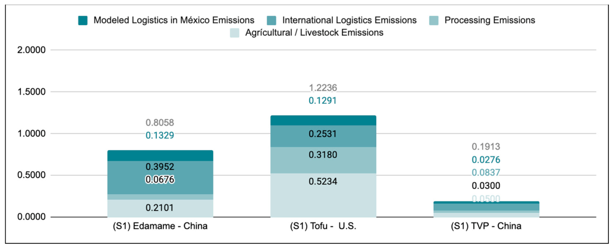
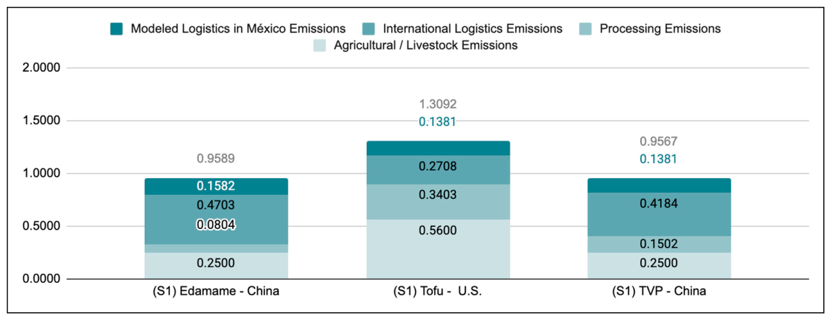
This configuration represents the existing operational constraints of the distribution network. In this scenario, all products are modeled as entering Mexican territory through the Nuevo Laredo, Tamaulipas, border crossing. (O→E→P→C→R→D) This gateway serves as the common origin node (O) for the domestic distribution. The corresponding environmental results are presented in

Table 12. Scenario 1 (S1), Edamame, Tofu, and TVP Results.

Scenario 1	Agricultural Emissions	Processing Emissions	Int. Logistics Emissions	Domestic Logistics Emissions	GWP (kg Product)	GWP (100 g Protein)
Edamame	0.2500	0.0804	0.4703	0.1582	0.9589	0.8058
Tofu	0.5600	0.3403	0.2708	0.1381	1.3092	1.2236
TVP	0.2500	0.1502	0.4184	0.1381	0.9567	0.1913

, while Figure 4 and Figure 5 illustrate GWP expressed per kilogram of product and per 100 g of delivered protein, respectively.

Edamame Baseline (Fujian, China): Recorded a functional GWP of 0.8058 kg CO₂e/100 g protein. The result reflects the combined contribution of international logistics and the continuous cold chain required across the multi-echelon distribution network. The mandatory transit through Nuevo Laredo (o), external (e), primary (p), and central (c) distribution centers prevents intermediate-node bypass and requires refrigerated transport and storage throughout the applicable stages. The impact per functional unit is further influenced by edamame’s relatively low protein concentration (11.9%).

Tofu Baseline (California, US): Recorded a functional GWP of 1.2236 kg CO₂e/100 g protein, the highest among the three products under S1. This result reflects its comparatively high agricultural and processing emissions, which together account for the largest share of its product-level GWP. International and domestic road transport further contribute to the total impact. When normalized to the functional unit, tofu’s low protein concentration (10.7%) amplifies these cumulative burdens, resulting in the highest GWP per 100 g of delivered protein under the baseline configuration.

TVP Baseline (Fujian, China): Recorded a functional GWP of 0.1913 kg CO₂e/100 g protein, the lowest among the three products under S1. Despite originating in the same region as edamame and undergoing long-distance international transport, TVP’s high protein concentration (50.0%) substantially reduces its impact when normalized to the functional unit. Its non-refrigerated distribution requirements further contribute to its comparatively low GWP, demonstrating the combined influence of protein density and product-specific logistics requirements on environmental performance.

This baseline configuration illustrates the environmental implications of rigid multi-echelon distribution structures, where mandatory handling and storage stages accumulate emissions regardless of product origin.

3.1.3. Scenario 2 (S2): Flexible Port Selection Network

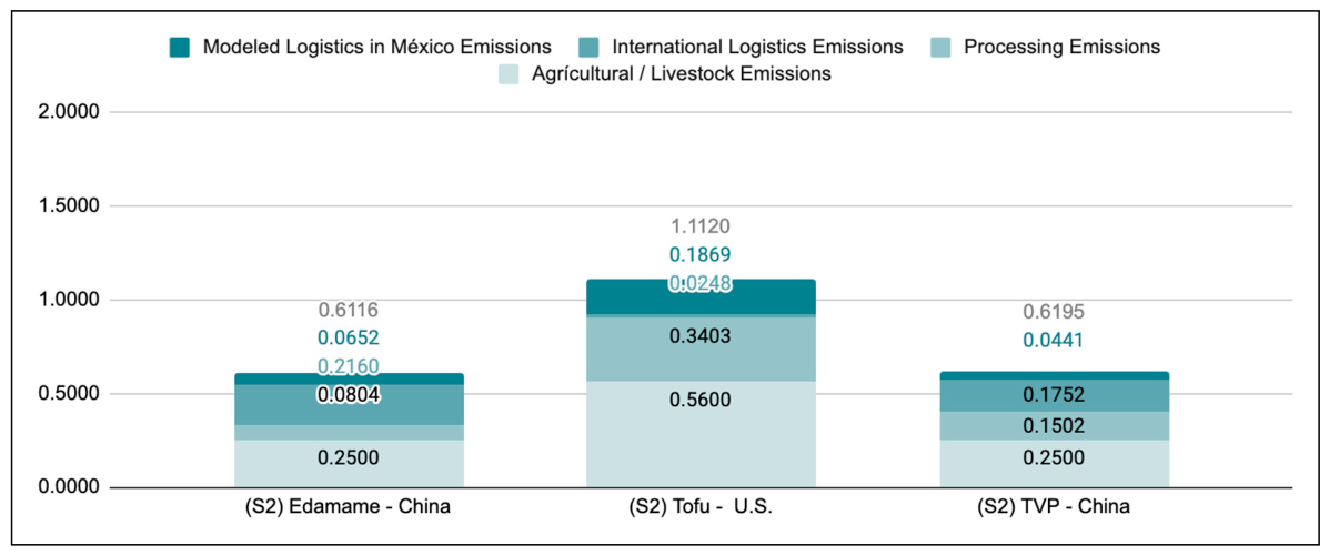
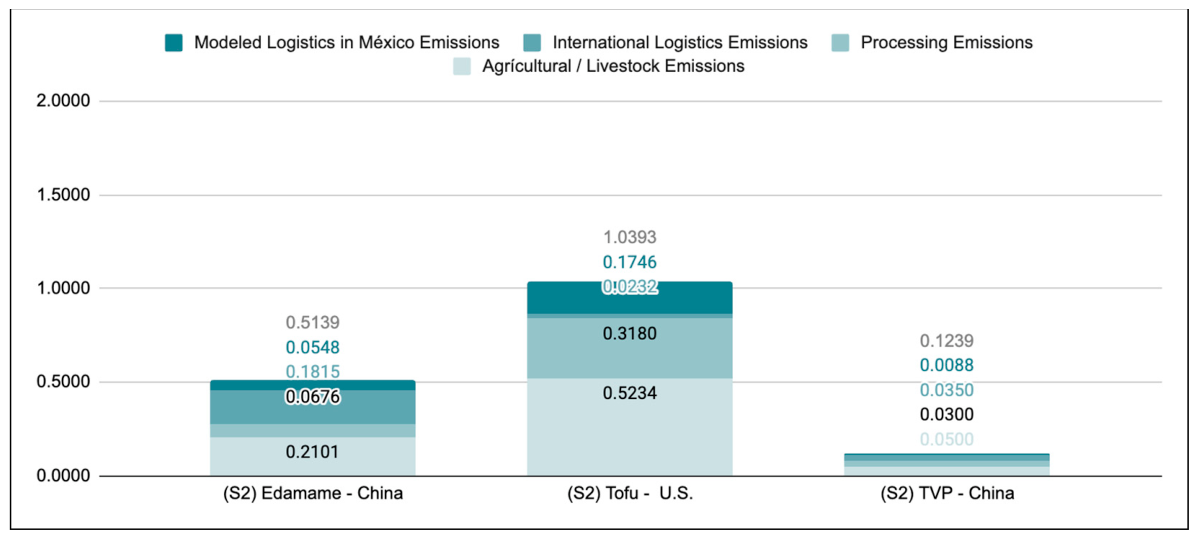
This configuration evaluates the environmental impact of endogenously selecting the optimal point of entry (o ∈ O) while maintaining the mandatory hierarchical distribution corridor (E→P→C). In this scenario, the solver is permitted to select among maritime ports or alternative border crossings based on the geographical origin of the products. Specifically, for edamame and TVP originating in China, the model identifies the port of Lázaro Cárdenas, Michoacán, as the optimal entry gateway. For tofu sourced from California, the model utilizes the Tijuana, Baja California border crossing. The corresponding environmental results are presented in

Table 13. Scenario 2 (S2), Edamame, Tofu, and TVP Results.

Scenario 2	Agricultural Emissions	Processing Emissions	Int. Logistics Emissions	Domestic Logistics Emissions	GWP (kg Product)	GWP (100 g Protein)
Edamame	0.2500	0.0804	0.2160	0.0652	0.6116	0.5139
Tofu	0.5600	0.3403	0.0248	0.1869	1.1120	1.0393
TVP	0.2500	0.1502	0.1752	0.0441	0.6195	0.1239

, while Figure 6 and Figure 7 illustrate GWP expressed per kilogram of product and per 100 g of delivered protein, respectively.

Edamame S2 (Fujian, China): The optimization of the entry gateway resulted in a functional GWP of 0.5139 kg CO₂e/100 g protein, representing a 36.2% reduction relative to the baseline. By endogenously selecting the Port of Lázaro Cárdenas instead of Nuevo Laredo, the model reduces both international and domestic logistics emissions while maintaining the same agricultural and processing conditions. The relatively low protein concentration (11.9%) nevertheless continues to amplify the impact when expressed per unit of delivered protein.

Tofu S2 (California, US): Recorded a functional GWP of 1.0393 kg CO₂e/100 g protein, representing a 15.1% reduction relative to the baseline. The Tijuana gateway reduces the international logistics burden associated with the California sourcing configuration. However, comparatively high agricultural and processing emissions, together with the low protein concentration (10.7%), result in tofu retaining the highest functional GWP among the three products under S2.

TVP S2 (Fujian, China): Achieved a functional GWP of 0.1239 kg CO₂e/100 g protein, representing a 35.2% reduction relative to the baseline. Selection of Lázaro Cárdenas reduces the logistics burden associated with the imported configuration. Although TVP exhibits a slightly higher GWP per kilogram of product than edamame under S2, its high protein concentration (50.0%) reverses this relationship on a nutritional basis, resulting in the lowest GWP per 100 g of delivered protein.

The results demonstrate that port-selection decisions can constitute an effective decarbonization strategy without requiring changes in suppliers, products, or distribution infrastructure. In this case, optimizing the point of entry generated substantial reductions in domestic transport burdens while preserving the existing network structure.

3.1.4. Scenario 3 (S3): Flexible Network with Intermediate-Node Bypass

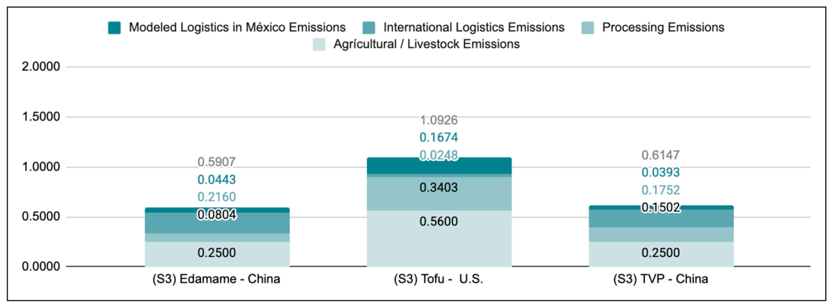
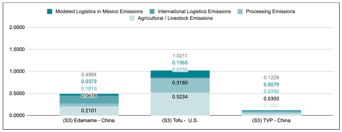
Scenario 3 evaluates the environmental implications of increased distribution-network flexibility by removing mandatory intermediate-node requirements. In this configuration, the solver is permitted to bypass the secondary echelons (E, P), allowing direct mass flows from the optimized origin nodes (O) to the central hub (C) or regional warehouses (R). This scenario evaluates the environmental implications of avoiding intermediate handling and storage stages. The corresponding environmental results are presented in

Table 14. Scenario 3 (S3), Edamame, Tofu, and TVP Results.

Scenario 3	Agricultural Emissions	Processing Emissions	Int. Logistics Emissions	Domestic Logistics Emissions	GWP (kg Product)	GWP (100 g Protein)
Edamame	0.2500	0.0804	0.2160	0.0443	0.5907	0.4964
Tofu	0.5600	0.3403	0.0248	0.1674	1.0926	1.0211
TVP	0.2500	0.1502	0.1752	0.0393	0.6147	0.1229

, while Figure 8 and Figure 9 illustrate GWP expressed per kilogram of product and per 100 g of delivered protein, respectively.

Edamame S3 (Fujian, China): Achieved a functional GWP of 0.4964 kg CO₂e/100 g protein, representing a 38.4% reduction relative to the baseline. Allowing intermediate-node bypass further reduces modeled domestic logistics emissions compared with S2, while agricultural, processing, and international logistics emissions remain unchanged. This indicates that additional routing flexibility can reduce the distribution burden of the frozen product by avoiding unnecessary intermediate handling and storage stages.

Tofu S3 (California, US): Recorded a functional GWP of 1.0211 kg CO₂e/100 g protein, representing a 16.5% reduction relative to the baseline. Although intermediate-node bypass reduces domestic logistics emissions compared with S2, the improvement is relatively modest because agricultural and processing emissions remain unchanged and constitute the dominant share of tofu’s total GWP. Combined with its low protein concentration (10.7%), these upstream burdens result in tofu retaining the highest functional GWP among the three products under S3.

TVP S3 (Fujian, China): Achieved a functional GWP of 0.1229 kg CO₂e/100 g protein, representing a 35.8% reduction relative to the baseline. Increased routing flexibility produces a further reduction in domestic logistics emissions compared with S2, although the change in total GWP is small because upstream agricultural, processing, and international logistics emissions remain unchanged.

The results demonstrate that intermediate-node bypass provides additional GWP reductions beyond those achieved through port selection alone, although the magnitude of the improvement varies across products. Because upstream sourcing conditions remain unchanged between S2 and S3, the observed reductions arise exclusively from changes in domestic network configuration. The comparatively small differences between S2 and S3 indicate that greater routing flexibility can further reduce distribution-stage emissions, but its influence on total cradle-to-retailer GWP depends on the relative contribution of logistics to each product’s overall environmental burden.

3.1.5. Scenario 4 (S4): National Sourcing and Hierarchical Distribution Framework

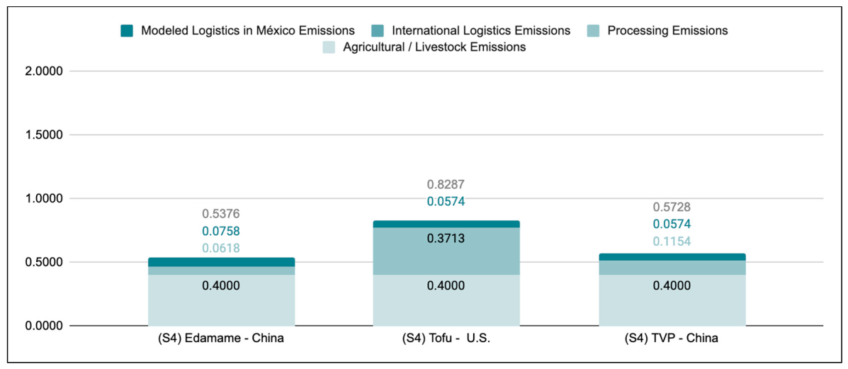
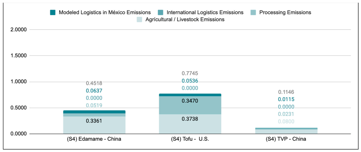
Scenario 4 evaluates the environmental implications of choosing a domestic supplier. To isolate the impact of sourcing geography from network topology, this configuration maintains the Hierarchical Distribution Framework (O→E→P→C→R→D) established in the empirical baseline. In this scenario, the origin node (O) is relocated to primary soybean-producing regions: Campeche, Chiapas, and Tamaulipas. In this configuration, all product manufacturing is modeled in Tamaulipas, identified as the optimal national origin node (O) due to its geographical proximity to the central distribution hubs. The corresponding environmental results are presented in

Table 15. Scenario 4 (S4), Edamame, Tofu, and TVP Results.

Scenario 4	Agricultural Emissions	Processing Emissions	Int. Logistics Emissions	Domestic Logistics Emissions	GWP (kg Product)	GWP (100 g Protein)
Edamame	0.4000	0.0618	0.0000	0.0758	0.5376	0.4518
Tofu	0.4000	0.3713	0.0000	0.0574	0.8287	0.7745
TVP	0.4000	0.1154	0.0000	0.0574	0.5728	0.1146

, while Figure 10 and Figure 11 illustrate GWP.

Edamame S4 (Tamaulipas, México): Recorded a functional GWP of 0.4518 kg CO₂e/100 g protein, representing a 43.9% reduction relative to the S1 baseline. Despite the higher agricultural emission factor assigned to domestic soybean production, the elimination of international logistics and the lower regionalized processing emissions more than offset this increase. Domestic sourcing therefore yields the lowest functional GWP observed for edamame across the four scenarios.

Tofu S4 (Tamaulipas, México): Recorded a functional GWP of 0.7745 kg CO₂e/100 g protein, representing a 36.7% reduction relative to the S1 baseline. Unlike edamame, domestic tofu exhibits lower agricultural emissions but slightly higher processing emissions than its U.S.-sourced counterpart, while international logistics emissions are eliminated. These changes produce the lowest GWP observed for tofu across the four scenarios, although its low protein concentration (10.7%) results in tofu retaining the highest functional GWP among the three products under S4.

TVP S4 (Tamaulipas, México): Achieved a functional GWP of 0.1146 kg CO₂e/100 g protein, representing a 40.1% reduction relative to the S1 baseline. Although the domestic agricultural emission factor is higher than that applied to the Chinese sourcing configuration, the elimination of international logistics and lower regionalized processing emissions reduce the total product-level impact. Combined with TVP’s high protein concentration (50.0%), these changes result in the lowest functional GWP observed across all products and scenarios evaluated in the study.

The scenario comparison shows that domestic sourcing (S4) yields the lowest functional GWP for all three products evaluated. However, this advantage does not result uniformly from lower upstream emission intensities. For edamame and TVP, the agricultural emission factor associated with domestic sourcing is higher than that of the corresponding Chinese sourcing configuration, but this increase is offset by the elimination of international logistics emissions, lower processing emissions, and changes in domestic distribution. Tofu similarly benefits from the elimination of international logistics and a lower agricultural emission factor, despite higher processing emissions under the domestic configuration. These results demonstrate that the environmental advantage of domestic sourcing emerges from the combined effects of sourcing-specific production characteristics, avoiding international transport, distribution-network configuration, and product protein density, rather than geographical proximity alone.

From a managerial perspective, the scenario comparison demonstrates that both sourcing geography and logistics-network design influence supply-chain emissions, although their relative importance varies across products. (S2) showed that port-selection decisions can reduce logistics-related impacts without requiring changes in suppliers or downstream infrastructure. Scenario 3 (S3) demonstrated that additional distribution flexibility and intermediate-node bypass can further reduce emissions by avoiding unnecessary handling and storage stages, although the incremental improvements relative to S2 were comparatively small. Finally, Scenario 4 (S4) demonstrated that domestic sourcing can provide substantial environmental benefits when evaluated together with regionalized production characteristics and the resulting logistics configuration, yielding the lowest functional GWP for all three products evaluated. Collectively, these findings indicate that sourcing, gateway selection, routing, and network-design decisions should be evaluated jointly rather than independently when developing lower-emission food supply chains.

3.1.6. Sensitivity Analysis

A sensitivity analysis was conducted using the rigid network configuration (S1) to evaluate the influence of four parameter groups: transportation emission factors, route distances, retailer demand, and upstream LCI emission factors. Each parameter was independently varied by ±10% while maintaining all other model inputs constant. Route-distance variations were applied to both international and domestic transportation, while upstream LCI sensitivity was evaluated by jointly varying agricultural and processing emission factors. The results are presented in

Table 16. Sensitivity analysis—kg CO₂eq/100 g of protein.

Parameter	Variation	Edamame	Δ%	Tofu	Δ%	TVP	Δ%
Baseline	—	0.8058	—	1.2236	—	0.1913	—
Transport EF	10%	0.8574	6.40%	1.2618	3.12%	0.2025	5.82%
Transport EF	−10%	0.7542	−6.40%	1.1854	−3.12%	0.1802	−5.82%
Retail Demand	10%	0.8383	4.03%	1.2570	2.73%	0.1985	3.74%
Retail Demand	−10%	0.7762	−3.67%	1.1932	−2.48%	0.1845	−3.57%
Route Distance	10%	0.8574	6.40%	1.2618	3.12%	0.2025	5.82%
Route Distance	−10%	0.7542	−6.40%	1.1854	−3.12%	0.1802	−5.82%
Upstream LCI EF	10%	0.8335	3.45%	1.3077	6.88%	0.1994	4.18%
Upstream LCI EF	−10%	0.7780	−3.45%	1.1395	−6.88%	0.1833	−4.18%

.

Variations in transportation emission factors and route distances produced the largest responses for edamame and TVP, reflecting the contribution of transport emissions to their S1 configurations. In contrast, tofu exhibited its greatest sensitivity to upstream LCI emission factors, consistent with the comparatively large contribution of agricultural and processing emissions to its total GWP. Retail demand variations produced smaller and slightly asymmetric changes because demand values are implemented as integer quantities in the optimization model. Despite these variations, the comparative environmental ranking remained unchanged under all tested conditions, with TVP consistently exhibiting the lowest GWP per functional unit, followed by edamame and tofu.

Overall, the sensitivity analysis indicates that the magnitude of GWP is influenced by different parameter groups depending on the product configuration, while the comparative ranking remains robust under moderate parameter variation. The product-specific responses further demonstrate that uncertainty in transport-related and upstream LCI inputs affects the evaluated products differently according to their underlying life-cycle emission profiles.

The targeted sensitivity tests showed a stronger response to changes in the maritime transport emission factor than to refrigerated storage intensity. For edamame, halving and doubling the maritime emission factor changed total GWP by −11.26% and +22.53%, respectively, while the corresponding changes for TVP were −9.16% and +18.31%. In contrast, halving and doubling the refrigerated storage emission factor changed edamame GWP by only −0.75% and +1.49%, respectively. These results in

Table 17. Targeted sensitivity tests—kg CO₂eq/100 g of protein.

Parameter	Product	Baseline	×0.5	Δ%	×2.0	Δ%
Maritime transport EF	Edamame S1	0.8058	0.7150	−11.26%	0.9873	22.53%
Maritime transport EF	TVP S1	0.1913	0.1738	−9.16%	0.2264	18.31%
Refrigerated storage EF	Edamame S1	0.8058	0.7997	−0.75%	0.8178	1.49%

indicate that, within the S1 configuration, total GWP is substantially more responsive to variation in maritime transport intensity than to refrigerated storage intensity.

3.2. Lifecycle Stage Contribution Analysis

The decomposition of the total GWP into discrete lifecycle stages (agricultural production, industrial processing, international logistics, and domestic distribution) examines the relative contribution of each stage across products and scenarios.

3.2.1. Upstream Production and Processing Intensities

Agricultural and processing emissions vary according to product and sourcing geography. Agricultural GWP ranges from 0.25 kg CO₂e/kg soybean for China to 0.56 for the United States, with 0.40 applied to domestic sourcing. Processing emissions are likewise geographically differentiated, reflecting product-specific energy requirements and regional electricity emission factors. These upstream differences contribute to the variation in total GWP across products and sourcing configurations.

3.2.2. Domestic Distribution Emissions

Domestic distribution emissions vary across products and network configurations, reflecting differences in point of entry, routing flexibility, intermediate-node utilization, and sourcing geography. Network flexibility reduces domestic logistics emissions substantially in several configurations, particularly under S2 and S3. Results are presented in

Table 18. Domestic distribution emissions (kg CO₂e/kg of product).

Product	S1	% S1	S2	% S2	S3	% S3	S4	% S4
Edamame	0.1582	16.5%	0.0652	10.7%	0.0443	7.5%	0.0758	14.1%
Tofu	0.1381	10.5%	0.1869	16.8%	0.1674	15.3%	0.0574	6.9%
TVP	0.1381	14.4%	0.0441	7.1%	0.0393	6.4%	0.0574	10.0%

.

Edamame: Domestic distribution emissions decreased from 0.1582 kg CO₂e/kg product in S1 to 0.0652 kg CO₂e/kg product in S2 and reached their minimum of 0.0443 kg CO₂e/kg product in S3. This progression demonstrates the effect of port selection and intermediate-node bypass on the distribution burden of a frozen product. Under domestic sourcing (S4), emissions increased slightly relative to S3 to 0.0758 kg CO₂e/kg product, but remained below the baseline.

Tofu: Domestic distribution emissions were 0.1381 kg CO₂e/kg product in S1 and increased to 0.1869 kg CO₂e/kg product in S2 before declining to 0.1674 kg CO₂e/kg product in S3. Unlike edamame, greater routing flexibility did not consistently reduce tofu’s domestic logistics burden because the alternative point of entry modified the distance traveled within the domestic network. Domestic sourcing (S4) produced the lowest value, at 0.0574 kg CO₂e/kg product.

TVP: Domestic distribution emissions decreased from 0.1381 kg CO2e/kg product in S1 to 0.0441 kg CO2e/kg product in S2 and reached their minimum of 0.0393 kg CO2e/kg product in S3. Under domestic sourcing (S4), emissions increased slightly relative to S3 to 0.0574 kg CO2e/kg product, but remained substantially below the baseline. Domestic distribution accounted for 14.4% of total product-level GWP in S1, 7.1% in S2, 6.4% in S3, and 10.0% in S4. The comparatively low domestic distribution burden of TVP reflects its non-refrigerated handling requirements, while its high protein concentration further reduces its environmental impact when results are expressed per 100 g of delivered protein.

Overall, S3 produced the lowest domestic distribution emissions for edamame and TVP, while S4 produced the lowest domestic distribution emissions for tofu. However, when the complete cradle-to-retailer system is considered, S4 achieved the lowest total GWP for all three products. This distinction highlights the value of the integrated LCA–LP framework: the network configuration that minimizes domestic logistics emissions does not necessarily minimize total life-cycle impacts, because sourcing-dependent agricultural, processing, and international transport emissions also influence overall environmental performance.

3.2.3. Influence of Functional Unit

Protein density strongly influences the comparative results under the selected functional unit, particularly for TVP (50.0% protein) relative to edamame (11.9%) and tofu (10.7%). However, this effect is specific to protein-based normalization; alternative functional units based on product mass, caloric value, or serving size could alter the relative environmental performance of the evaluated products.

4. Discussion

4.1. Discussion

This study evaluated how sourcing geography and distribution-network structure influence cradle-to-retailer GWP in soy-derived protein supply chains by integrating attributional LCA with LP network optimization. Four sourcing and distribution configurations were evaluated for edamame, tofu, and TVP under identical demand conditions. The results demonstrate that both sourcing geography and network configuration influence environmental performance, although their relative importance varies across products. Domestic sourcing (S4) yielded the lowest functional GWP for all three products, while intermediate-node bypass (S3) minimized domestic distribution emissions for edamame and TVP. This distinction demonstrates that minimizing logistics emissions alone does not necessarily minimize total cradle-to-retailer GWP, as agricultural production, processing, and international transport also influence overall performance.

Tofu exhibited the highest baseline GWP (1.2236 kg CO₂e/100 g protein), whereas domestically sourced TVP achieved the lowest impact across all evaluated configurations (0.1146 kg CO₂e/100 g protein). Protein density strongly influenced comparative performance under the selected functional unit, particularly for TVP. Sensitivity analysis confirmed that the product ranking remained stable under moderate variations in transport emission factors, route distances, demand, and upstream LCI parameters.

These findings complement previous research on the environmental relevance of transport and cold-chain operations in food supply chains [2,12,49], while the influence of protein-based normalization is consistent with nutritional LCA research on soy-based products and protein functional units [10,13]. The results further support the value of integrating LCA and supply-chain optimization to evaluate environmental performance across interconnected sourcing and routing decisions [16].

4.2. Managerial and Academic Implications

From a managerial perspective, the revised results support domestic sourcing as the lowest-GWP procurement strategy across the evaluated products, although the magnitude and source of the benefit vary by product. For frozen edamame, procurement strategies should combine domestic sourcing with reductions in temperature-controlled transport and intermediate storage; for tofu, shorter domestic road-distribution distances provide the principal logistical advantage; and for TVP, domestic sourcing complements its lower distribution burden associated with non-refrigerated handling and higher protein density. Flexible port selection, intermediate-node bypass, and avoidance of unnecessary storage stages can further reduce distribution emissions. Accordingly, sourcing and distribution decisions should be evaluated jointly rather than as independent decarbonization strategies.

From a policy perspective, the results indicate that decarbonization strategies should consider both sourcing geography and logistics-network design. Investments in flexible logistics infrastructure, decentralized distribution, and cold-chain efficiency may complement domestic sourcing, particularly in contexts such as Mexico where long-haul road transport is important to national food distribution.

From an academic standpoint, the study demonstrates the analytical value of integrating LCA with network optimization to distinguish sourcing-dependent life-cycle burdens from routing-dependent distribution emissions. The framework provides a decision-support approach for evaluating lower-emission food supply-chain configurations.

Beyond the evaluated case study, the proposed framework contributes to the design of more sustainable food supply chains by enabling evidence-based sourcing and logistics-network design decisions that reduce environmental impacts in temperature-controlled food supply chains.

4.3. Future Research

Several extensions may strengthen the robustness and applicability of the present framework.

(1) LCA Validation and Uncertainty: Future research could validate the results using dedicated LCA software and background databases, enabling Monte Carlo uncertainty analysis and dynamic LCA to incorporate temporal changes in electricity mixes, transportation performance, and other inventory parameters.

(2) Mixed-Integer Linear Programming (MILP) and Alternative Logistics: Extending the model to MILP would enable discrete decisions such as facility siting, fleet sizing, rail intermodal transport, and regional processing configurations.

(3) Multi-Objective Optimization and Economic Trade-offs: A multi-objective formulation incorporating GWP and logistics costs could quantify environmental–economic trade-offs and support more comprehensive supply-chain decisions.

(4) Operational Uncertainty and Product Losses: Future models could incorporate stochastic demand and lead times, product- and node-specific loss and spoilage rates, and vehicle loading conditions to evaluate the resilience of optimized routes under operational variability.

(5) Policy and Scale-Oriented Scenarios: Future applications could incorporate agricultural subsidies, import tariffs, carbon pricing, procurement scale, and retailer coverage to evaluate how policy interventions and network expansion.

4.4. Limitations

Several limitations should be acknowledged when interpreting the results of the present study. First, the deterministic model does not capture stochastic variability in demand, congestion, lead times, or operational disruptions, while procurement scale and retailer coverage were held constant across scenarios. Transport emission factors were also treated as constant by mode and temperature-control condition; shipment-specific loading, empty backhauls, traffic, climatic, driver-related, and temporal variability were not explicitly modeled. Product- and node-specific losses and spoilage were excluded because case-specific data were unavailable.

Second, despite the geographical differentiation introduced into the agricultural inventory, regional LCI data remains uneven. China and U.S. agricultural factors were derived from country-specific studies, while the Mexican inventory was reconstructed for southern Tamaulipas using regional foreground data and multiple emission-factor sources. Equivalent foreground inventories were unavailable for Chiapas and Campeche, and some agricultural and processing inputs relied on literature-derived proxies. Consequently, residual regional uncertainty may influence absolute GWP estimates. Sensitivity analysis evaluated selected parameters, but probabilistic uncertainty propagation across the complete inventory was not performed.

Third, infrastructure locations and distribution nodes were fixed, and the model was formulated as a single-objective GWP optimization. It therefore does not quantify environmental–economic trade-offs or evaluate alternative strategies such as rail intermodal transport.

Finally, the primary functional unit was 100 g of delivered protein, complemented by results per kilogram of product. Alternative normalization by caloric value, edible portion, or serving size may produce different comparative relationships. The assessment was limited to GWP100 and therefore excludes other impact categories such as eutrophication, acidification, land use, and water consumption. The cradle-to-retailer boundary also excludes retail activities, consumer use, post-retailer food waste, and end-of-life management. Accordingly, the results represent comparative assessments of the evaluated sourcing and network configurations rather than complete product life cycles.

References

1. Crippa, M.; Solazzo, E.; Guizzardi, D.; Monforti-Ferrario, F.; Tubiello, F.N.; Leip, A. Food Systems are Responsible for a Third of Global Anthropogenic GHG Emissions. Nat. Food 2021, 2, 198–209. [Google Scholar] [CrossRef] [Scilit] [PubMed]
2. Li, M.; Jia, N.; Lenzen, M.; Malik, A.; Wei, L.; Jin, Y.; Raubenheimer, D. Global Food-Miles Account for nearly 20% of Total Food-Systems Emissions. Nat. Food 2022, 3, 445–453. [Google Scholar] [CrossRef] [Scilit] [PubMed]
3. Intergovernmental Panel on Climate Change (IPCC). Climate Change 2013: The Physical Science Basis. Contribution of Working Group I to the Fifth Assessment Report of the Intergovernmental Panel on Climate Change; Cambridge University Press: Cambridge, UK; New York, NY, USA, 2013; Available online: https://www.ipcc.ch/report/ar5/wg1/ (accessed on 8 July 2026).
4. Mckinnon, A.C. Decarbonizing Logistics: Distributing Goods in a Low-Carbon World; Kogan Page: London, UK, 2018. [Google Scholar]
5. International Transport Forum. ITF Transport Outlook 2021; OECD Publishing: Paris, France, 2021. [Google Scholar] [CrossRef] [Scilit]
6. OECD. Review of the Regulation of Freight Transport in Mexico; OECD Publishing: Paris, France, 2017. [Google Scholar] [CrossRef] [Scilit]
7. Sims, R.; Schaeffer, R.; Creutzig, F.; Cruz-Núñez, X.; D’Agosto, M.; Dimitriu, D.; Figueroa Meza, M.J.; Fulton, L.; Kobayashi, S.; Lah, O.; et al. Climate Change 2014: Mitigation of Climate Change. Contribution of Working Group III to the Fifth Assessment Report of the Intergovernmental Panel on Climate Change; Chapter 8: Transport; Cambridge University Press: Cambridge, UK; New York, NY, USA, 2014; pp. 599–670. [Google Scholar] [CrossRef] [Scilit]
8. Pro-Nuño, A.; Torres, E.G.; Ruiz-Morales, M. Catching Up with the Food Supply Cold Chain in the Post-Pandemic Context: A Literature Review. J. Food Process Eng. 2025, 48, e70152. [Google Scholar] [CrossRef] [Scilit]
9. Poore, J.; Nemecek, T. Reducing Food’s Environmental Impacts through Producers and Consumers. Science 2018, 360, 987–992. [Google Scholar] [CrossRef] [Scilit] [PubMed]
10. Herrmann, M.; Wilfart, A.; Aubin, J.; Fischer, M.; Voget-Kleschin, L.; Teigiserova, D.A. A Comparative Nutritional Life Cycle Assessment of Soy-Based Products and a Processed Soy-Based Meat Analogue. Front. Sustain. Food Syst. 2024, 8, 1413802. [Google Scholar] [CrossRef] [Scilit]
11. Mccarthy, D.; Matopoulos, A.; Davies, P. Life Cycle Assessment in the Food Supply Chain: A Case Study. Int. J. Logist. Res. Appl. 2015, 18, 140–154. [Google Scholar] [CrossRef] [Scilit]
12. Karacan, M.A.; Yilmaz, I.C.; Yilmaz, D. Key Implications on Food Storage in Cold Chain by Energy Management Perspectives. Front. Sustain. Food Syst. 2023, 7, 1250646. [Google Scholar] [CrossRef] [Scilit]
13. Mcauliffe, G.A.; Takahashi, T.; Beal, T.; Huppertz, T.; Leroy, F.; Buttriss, J.; Collins, A.L.; Drewnowski, A.; Mclaren, S.J.; Ortenzi, F. Protein Quality in Life Cycle Assessment. Int. J. Life Cycle Assessment. 2023, 28, 146–155. [Google Scholar] [CrossRef] [Scilit] [PubMed]
14. ISO 14040:2006; Environmental Management—Life Cycle Assessment—Principles and Framework. International Organization for Standardization: Geneva, Switzerland, 2006.
15. ISO 14044:2006; Environmental Management—Life Cycle Assessment—Requirements and Guidelines. International Organization for Standardization: Geneva, Switzerland, 2006.
16. Hülagü, S.; Dullaert, W.; Eruguz, A.S.; Heijungs, R.; Inghels, D. Integrating Life Cycle Assessment into Chain Optimization. PLoS ONE 2025, 20, e0316710. [Google Scholar] [CrossRef] [Scilit] [PubMed]
17. Liao, C.; Hsu, H. A Multi-Objective Supply Chain Model for Reducing Carbon Emissions and Food Losses in a Multi-Period Mixed Product Environment. Socio-Econ. Plan. Sci. 2025, 101, 102285. [Google Scholar] [CrossRef] [Scilit]
18. Flores-Siguenza, P.; Lopez-Sanchez, V.; Mosquera-Gutierres, J.; Llivisaca-Villazhañay, J.; Moscoso-Martínez, M.; Guamán, R. Fuzzy Optimization and Life Cycle Assessment for Sustainable Supply Chain Design: Applications in the Dairy Industry. Sustainability 2025, 17, 5634. [Google Scholar] [CrossRef] [Scilit]
19. Astudillo, M.F.; Krämer, K.; Arteaga, A. Using Dynamic Life Cycle Assessment to Evaluate the Effects of Industry Digitalization: A Steel Case Study. J. Ind. Ecol. 2024, 28, 942–952. [Google Scholar] [CrossRef] [Scilit]
20. Liu, Y.; Huang, Z.; Luo, X.; Ma, H.; Li, Z. Insights of airborne transmission within urban rail transit carriage environments after the COVID-19 pandemic. Indoor Built Environ. 2026, 35, 1011–1040. [Google Scholar] [CrossRef] [Scilit]
21. Huang, Z.; Liu, Y.; Ma, H.; Luo, X.; Li, Z. Numerical Investigation of Exhaled Droplet Transmission and Infection Probability Prediction in a Subway Compartment Under Ventilation and Passenger Effects with an Improved Wells-Riley Equation. Int. J. Heat Mass Transf. 2026, 265, 128809. [Google Scholar] [CrossRef] [Scilit]
22. United States Department of Agriculture, Foreign Agricultural Service (USDA-FAS). Oilseeds and Products Annual—Mexico. 2026. Available online: https://apps.fas.usda.gov/newgainapi/api/Report/DownloadReportByFileName?fileName=Oilseeds+and+Products+Annual_Mexico+City_Mexico_MX2026-0020 (accessed on 11 July 2026).
23. Servicio de Información Agroalimentaria y Pesquera (SIAP). Avances De Siembras Y Cosechas: Oleaginosas—Soya. 2023. Available online: https://www.gob.mx/agricultura%7Cdgsiap/articulos/avances-de-siembras-y-cosechas-y-de-la-produccion-pecuaria2 (accessed on 11 July 2026).
24. Springer, N.P. Explaining Global Variation in Life-Cycle Greenhouse Gas Emissions from Soybeans and Soybean Meal: A Systematic Review. Agric. Syst. 2026, 233, 104559. [Google Scholar] [CrossRef] [Scilit]
25. Lucić, R.; Raposo, M.; Chervinska, A.; Domingos, T.; Teixeira, R.F.M. Global Greenhouse Gas Emissions and Land use Impacts of Soybean Production: Systematic Review and Analysis. Sustainability 2025, 17, 3396. [Google Scholar] [CrossRef] [Scilit]
26. Schaubroeck, T. Relevance of Attributional and Consequential Life Cycle Assessment for Society and Decision Support. Front. Sustain. 2023, 4, 1063583. [Google Scholar] [CrossRef] [Scilit]
27. Brito, T.; Fragoso, R.; Santos, L.; Martins, J.A.; Fernandes Silva, A.A.; Aranha, J. Life Cycle Assessment for Soybean Supply Chain: A Case Study of State of Pará. Brazil. Agronomy 2023, 13, 1648. [Google Scholar] [CrossRef] [Scilit]
28. du Plessis, M.J.; van Eeden, J.; Goedhals-Gerber, L.L. The Carbon Footprint of Fruit Storage: A Case Study of the Energy and Emission Intensity of Cold Stores. Sustainability 2022, 14, 7530. [Google Scholar] [CrossRef] [Scilit]
29. Rybak, K.; Parniakov, O.; Samborska, K.; Wiktor, A.; Witrowa-Rajchert, D.; Nowacka, M. Energy and Quality Aspects of Freeze-Drying Preceded by Traditional and Novel Pre-Treatment Methods as Exemplified by Red Bell Pepper. Sustainability 2021, 13, 2035. [Google Scholar] [CrossRef] [Scilit]
30. Ning, G.; Yang, F.; Zhao, J.; Wang, S. Spatiotemporal Analysis of the Carbon Footprint of Soybean Production in China Based on Life Cycle Assessment. Foods 2026, 15, 1979. [Google Scholar] [CrossRef] [Scilit] [PubMed]
31. Romeiko, X.X.; Lee, E.K.; Sorunmu, Y.; Zhang, X. Spatially and Temporally Explicit Life Cycle Environmental Impacts of Soybean Production in the U.S. Midwest. Environ. Sci. Technol. 2020, 54, 4758–4768. [Google Scholar] [CrossRef] [Scilit] [PubMed]
32. Fideicomisos Instituidos en Relación con la Agricultura (FIRA). Sistema De Costos Agrícolas: Soya, Tecnología TMF, Modalidad Tradicional, Sur De Tamaulipas, Ciclo PV 2017; Fideicomisos Instituidos en Relación con la Agricultura (FIRA): Morelia, Mexico, 2017. [Google Scholar]
33. Pereira, L.G.; Ramos, N.P.; Pighinelli, A.L.M.T.; Novaes, R.M.L.; Seabra, J.E.A.; Debiasi, H.; Hirakuri, M.H.; Folegatti, M.I.S. State-Level Inventories and Life Cycle GHG Emissions of Corn, Soybean, and Sugarcane Produced in Brazil. Sustainability 2025, 17, 8482. [Google Scholar] [CrossRef] [Scilit]
34. Sánchez-Morales, P.; Romero-Arenas, O. Fossil Fuels and CO2e in Traditional Milpa and Monoculture Maize Systems in Tlaxcala, Mexico. Rev. Mex. DE Cienc. Agríc. 2017, 8, 919–932. [Google Scholar] [CrossRef] [Scilit]
35. Secretaría de Medio Ambiente y Recursos Naturales (SEMARNAT), Gobierno de México, México. Factores De Emisión 2015. Available online: https://www.gob.mx/cms/uploads/attachment/file/235891/FACTORES_DE_EMISION_2015.pdf (accessed on 18 July 2026).
36. Prussi, M.; Yugo, M.; De Prada, L.; Padella, M.; Edwards, R. JEC Well-to-Tank Report V5: Well-to-Wheels Analysis of Future Automotive Fuels and Powertrains in the European Context; Publications Office of the European Union: Luxembourg, 2020. [Google Scholar] [CrossRef] [PubMed]
37. Intergovernmental Panel on Climate Change (IPCC). 2019 Refinement to the 2006 IPCC Guidelines for National Greenhouse Gas Inventories. 2019. Available online: https://www.ipcc.ch/report/2019-refinement-to-the-2006-ipcc-guidelines-for-national-greenhouse-gas-inventories/ (accessed on 14 July 2026).
38. Andersen, M.S.; Bonnis, G. Climate Mitigation Co-Benefits from Sustainable Nutrient Management in Agriculture: Incentives and Opportunities; OECD Environment Working Papers 2021, No. 186; OECD Publishing: Paris, France, 2021. [Google Scholar] [CrossRef]
39. Mejía, A.; Harwatt, H.; Jaceldo-Siegl, K.; Sranacharoenpong, K.; Soret, S.; Sabaté, J. Greenhouse Gas Emissions Generated by Tofu Production: A Case Study. J. Hunger. Amp Environ. Nutr. 2018, 13, 131–142. [Google Scholar] [CrossRef] [Scilit]
40. Saerens, W.; Smetana, S.; Van Campenhout, L.; Lammers, V.; Heinz, V. Life Cycle Assessment of Burger Patties Produced with Extruded Meat Substitutes. J. Clean. Prod. 2021, 306, 127177. [Google Scholar] [CrossRef] [Scilit]
41. Wróbel-Jędrzejewska, M.; Polak, E. Determination of Carbon Footprint in the Processing of Frozen Vegetables using an Online Energy Measurement System. J. Food Eng. 2022, 322, 110974. [Google Scholar] [CrossRef] [Scilit]
42. Comisión Reguladora de Energía (CRE); Secretaría de Medio Ambiente y Recursos Naturales (SEMARNAT). Factor De Emisión Del Sistema Eléctrico Nacional 2024. Available online: https://www.gob.mx/cms/uploads/attachment/file/980977/AvisoFESEN_2024.pdf (accessed on 16 July 2026).
43. Ministry of Ecology and Environment of the People’s Republic of China; National Bureau of Statistics of China; National Energy Administration. National Electricity Carbon Footprint Factors for 2024. Announcement No. 19 of 2025, 2025. Available online: https://www.mee.gov.cn/xxgk2018/xxgk/xxgk01/202510/t20251024_1130734.html (accessed on 1 August 2026).
44. United States Environmental Protection Agency (EPA). eGRID Summary Tables 2023. Available online: https://www.epa.gov/egrid/summary-data (accessed on 2 August 2026).
45. United States Environmental Protection Agency (EPA). Emission Factors for Greenhouse Gas Inventories. 2023. Available online: https://www.epa.gov/climateleadership/ghg-emission-factors-hub (accessed on 2 August 2026).
46. Fitzgerald, W.B.; Howitt, O.J.A.; Smith, I.J.; Hume, A. Energy use of Integral Refrigerated Containers in Maritime Transportation. Energy Policy 2011, 39, 1885–1896. [Google Scholar] [CrossRef] [Scilit]
47. Serrano-Guevara, O.S.; Huertas, J.I.; Quirama, L.F.; Mogro, A.E. Energy Efficiency of Heavy-Duty Vehicles in Mexico. Energies 2022, 16, 459. [Google Scholar] [CrossRef] [Scilit]
48. Du Plessis, M.J.; Van Eeden, J.; Goedhals-Gerber, L.; Else, J. Calculating Fuel Usage and Emissions for Refrigerated Road Transport using Real-World Data. Transp. Res. Part D Transp. Environ. 2023, 117, 103623. [Google Scholar] [CrossRef] [Scilit]
49. James, S.J.; James, C. The Food Cold-Chain and Climate Change. Food Res. Int. 2010, 43, 1944–1956. [Google Scholar] [CrossRef] [Scilit]
50. Secretaría de Energía (SENER). Atlas Nacional De Zonas Con Alto Potencial De Energías Limpias. 2024. Available online: https://www.gob.mx/sener/articulos/atlas-nacional-de-zonas-con-alto-potencial-de-energias-limpias (accessed on 21 July 2026).
51. Secretaría de Energía (SENER). NORMA Oficial Mexicana NOM-001-SEDE-2012, Instalaciones Eléctricas (Utilización). 2012. Available online: https://sidof.segob.gob.mx/notas/5280607 (accessed on 23 July 2026).
52. IEC 61724-1:2021; Photovoltaic System Performance—Part 1: Monitoring, 2nd ed. IEC: Geneva, Switzerland, 2021. Available online: https://webstore.iec.ch/en/publication/65561 (accessed on 22 July 2026).
53. Du Plessis, M.; Van Eeden, J.; Goedhals-Gerber, L.L. Energy and Emissions: Comparing Short and Long Fruit Cold Chains. Heliyon 2024, 10, e32507. [Google Scholar] [CrossRef] [Scilit] [PubMed]
54. Hassan, R.; Gurning, R.O.S.; Handani, D.W. Analysis of the Container Dwell Time at Container Terminal by using Simulation Modelling. Int. J. Mar. Eng. Innov. Res. 2020, 5, 34–43. [Google Scholar] [CrossRef] [Scilit]
55. Filina-Dawidowicz, L.; Filin, S. Innovative Energy-Saving Technology in Refrigerated Containers Transportation. Energy Effic. 2019, 12, 1151–1165. [Google Scholar] [CrossRef] [Scilit]
56. United States Department of Agriculture (USDA). Vegetables and Pulses Yearbook Data—Edamame. 2022. Available online: https://www.ers.usda.gov/data-products/vegetables-and-pulses-data/vegetables-and-pulses-yearbook-tables (accessed on 3 August 2026).
Figure 1. Superstructure—Edamame Baseline Scenario (S1).
Sustainability 18 08667 g001
Figure 2. Case Study—Edamame (S1), Tofu (S1), and TVP (S4). Red dashed lines represent maritime transport routes, while black lines represent road transport routes.
Sustainability 18 08667 g002
Figure 3. Domestic Distribution Network.
Sustainability 18 08667 g003
Figure 4. (S1) Results—kg CO2eq/kg of product.
Sustainability 18 08667 g004
Figure 5. (S1) Results—kg CO2eq/100 g of protein.
Sustainability 18 08667 g005
Figure 6. (S2) Results—kg CO2eq/kg of product.
Sustainability 18 08667 g006
Figure 7. (S2) Results—kg CO2eq/100 g of protein.
Sustainability 18 08667 g007
Figure 8. (S3) Results—kg CO2eq/kg of product.
Sustainability 18 08667 g008
Figure 9. (S3) Results—kg CO2eq/100 g of protein.
Sustainability 18 08667 g009
Figure 10. (S4) Results—kg CO2eq/kg of product.
Sustainability 18 08667 g010
Figure 11. (S4) Results—kg CO2eq/100 g of protein.
Sustainability 18 08667 g011