Article

Linking Multi-Scale Stressors to Fish and Benthic Invertebrates in Non-Wadable Rivers: Implications for River Management


1
Institute for Water of the Republic of Slovenia, Einspielerjeva ulica 6, 1000 Ljubljana, Slovenia
2
Department of Biology, Biotechnical Faculty, University of Ljubljana, Jamnikarjeva 101, 1000 Ljubljana, Slovenia
*
Authors to whom correspondence should be addressed.
Sustainability 2026, 18(17), 8613; https://doi.org/10.3390/su18178613
Submission received: 15 June 2026 / Revised: 17 August 2026 / Accepted: 21 August 2026 / Published: 22 August 2026
(This article belongs to the Section Sustainability, Biodiversity and Conservation)

Abstract

Understanding how multiple stressors operating across spatial scales shape riverine biota is essential for advancing sustainable ecosystem management. This study evaluated the relative importance of hydromorphological alterations and land-use changes for benthic invertebrate (n = 77) and fish assemblages (n = 92) in large Slovenian rivers. Multivariate analyses were employed to disentangle unique and shared effects of stressors at reach, segment, and catchment scales while accounting for natural variability. The results revealed a hierarchical structuring of stressors, with regional factors shaping local conditions. Fish assemblages were predominantly associated with local-scale stressors, particularly at the segment scale, whereas benthic invertebrates were more strongly associated with shared stressor effects across multiple spatial scales. Stressors explained substantially more variability in fish (43.5%) than in benthic invertebrates (19.9%). Catchment-scale land use showed higher explanatory power than local riparian land use. Typological variables moderately improved model performance, emphasizing the contribution of natural environmental gradients. Our findings suggest that large river management may benefit from a multi-scale perspective that prioritizes segment-scale habitat conditions for fish and coordinated catchment-to-local strategies for benthic invertebrates, with potential benefits for ecosystem resilience and long-term sustainability.

1. Introduction

River ecosystems in Europe are increasingly affected by multiple anthropogenic stressors, leading to widespread alterations of their morphology, hydrological regimes, physico-chemical conditions, and their biological communities. Because river ecosystems are hierarchically organized, with local-scale habitat characteristics co-shaped by broader regional-scale drivers such as geology, topography, climate, and land use/cover, understanding the responses (the structure and functioning) of river ecosystems to anthropogenic change requires a comprehensive assessment of environmental factors operating across multiple spatial scales [1,2,3].
Previous studies have examined the relative importance of stressors acting at different spatial scales, but generally applicable conclusions remain elusive, as reported effects vary among regions, organism groups, and analytical approaches [4,5,6,7,8,9,10,11]. This highlights the need for further studies focusing on specific geographical regions, river types, and/or environmental contexts to derive ecologically meaningful and management-relevant conclusions [12,13]. This need is particularly relevant for non-wadable rivers, because their greater size, discharge, and habitat heterogeneity support distinct biological assemblages, integrate environmental influences over broader spatial scales, and require specialized sampling approaches compared with wadable streams [14,15,16].
Anthropogenic stressors acting on river ecosystems are commonly grouped into pollution-related, land use-related, and hydromorphology-related stressors. Identifying the relative influence of these stressors on aquatic assemblages is often challenging due to strong collinearity between stressor variables and natural environmental gradients [17,18]. Moreover, when multiple stressors with similar ecological effects act simultaneously, it becomes difficult to disentangle the individual contribution of each stressor [17]. Stressors may also interact in complex ways, producing synergistic, antagonistic, or reversal effects that differ from the simple sum of their individual (additive) impacts [19,20,21,22]. Therefore, understanding the combined influence of multiple interacting stressors is essential. Additionally, different organism groups may respond differently to the same individual or combined stressors [23,24]. Relying on a single assemblage (for example, fish) as an ecological indicator may thus fail to reflect the broader structural and functional responses of the ecosystem [6]. By integrating multiple organism groups with varying sensitivities and ecological roles, the likelihood of detecting the most relevant stressor effects in riverine ecosystems is substantially improved. This principle underlies the conceptual framework set by the Water Framework Directive (WFD) in Europe, where the ecological status of surface waters is determined by considering a mandatory set of type-specific biological indicators (or quality elements).
Hydromorphological conditions play a central role in structuring aquatic communities and regulating ecosystem functioning in river systems [3,25]. For example, flow regime, channel morphology, longitudinal, lateral, and vertical connectivity govern habitat availability, sediment dynamics, and the transport of organisms, organic matter, and nutrients, thereby shaping species composition and life-history processes [26,27,28]. Hydromorphological alterations such as dam construction, channelization, water abstraction, and riparian vegetation removal disrupt these processes by constraining lateral channel migration, accelerating flow velocities, altering sediment inputs, and reducing connectivity with floodplains and the hyporheic zone [29,30,31,32]. These effects are particularly pronounced in large floodplain rivers, where extensive lateral connectivity and habitat diversity underpin high biodiversity and productivity [33,34]. As a result, hydromorphological degradation leads to habitat loss and homogenization, impaired migration and recolonization, altered disturbance regimes, and ultimately reduced diversity and altered structure of aquatic communities [14,35,36,37,38,39].
In addition to hydromorphological pressures, land-use change is often recognized as an important driver of ecological change in river ecosystems. However, studies have found that the intensity and nature of the effects of land-use change depend significantly on the spatial proximity of these changes to the river network (positioning) and the spatial extent over which they occur [40], as well as on contextual factors such as land-cover reference conditions (historical vegetation cover) and type of land-use conversion [41,42,43]. The conversion of natural vegetation to agricultural or urban land use can directly alter ecosystem structure and functioning through changes in organic matter inputs (e.g., fallen leaves and branches), riparian shading, and thermal regimes. These modifications can, in turn, affect habitat availability, food resources, and primary production. In addition, land-use change exerts indirect effects by altering runoff dynamics, intensifying stormwater hydrology, and increasing the delivery of fine sediments, nutrients, and contaminants. Such changes lead to degradation of physical habitat structure, typically manifested as habitat simplification and homogenization, increased flow variability, and reduced water quality [13,44,45,46,47].
Although hydromorphological stressors and land-use-related pressures originate from different underlying drivers, they often result in similar effects on the physical characteristics of river habitats. As these pressures most often co-occur and act on biological communities through overlapping pathways, it is important to consider them both in pressure-response studies.
Achieving “good” ecological status for all surface water bodies is the central objective of the WFD. However, the majority of large European rivers currently fail to meet this objective, implying that significant efforts will be needed to improve their ecological condition in the coming years [48]. To effectively guide river management and restoration strategies, it is crucial to understand whether local restoration measures—implemented at smaller spatial scales—can meaningfully improve the ecological status of rivers. Several studies have shown that improvements in habitat quality at small spatial extents often result in only marginal biological responses, or, in some cases, no detectable improvements in aquatic assemblages [49,50,51,52]. A common reason for this ecological failure is the spatial mismatch between the scale of intervention and the spatial scale at which key environmental drivers influence aquatic biota [53]. Therefore, identifying the most relevant stressors and the spatial scales at which they operate is a fundamental prerequisite for designing effective management actions aimed at improving or maintaining the ecological status of large river ecosystems [54,55]. Accordingly, identifying associations between biological assemblages and local, broader-scale, and cross-scale stressors can provide a basis for considering whether broader-scale pressures may constrain the potential effectiveness of local restorations.
The present study advances current knowledge by focusing specifically on large non-wadable rivers in the Danube River Basin, a river category that remains comparatively underrepresented in multi-scale ecological studies. The dataset covers broad gradients of hydromorphological alteration and riparian land-use intensity, ranging from nearly natural to severely modified conditions, which are rarely available for large European rivers. At the same time, the generally good water quality and relatively narrow water-quality gradient provide a context in which associations with hydromorphological and land-use stressors can be examined without a dominant pollution gradient. The study extends previous scale-selection work by using predefined local spatial scales within a broader hierarchical framework that additionally incorporates catchment-scale stressors and natural typological variables. Furthermore, the study jointly compares fish and benthic invertebrates and applies variance partitioning to quantify the unique and shared contributions of the predictor groups.
The main objective of this study was to quantify the relative importance of hydromorphological modification and land-use change in structuring benthic invertebrate and fish assemblages in non-wadable river systems. We specifically examined how the influence of stressor variables differs across spatial scales (reach, segment, and catchment) and to what extent local versus broad-scale drivers dominate in explaining biological variability. In addition, we partitioned the unique and shared contributions of multiple stressor groups to determine whether patterns in aquatic assemblages are driven predominantly by distinct local or regional pressures or by their combined effects across multiple spatial scales. We further evaluated the role of natural typological variables, such as catchment size, altitude, and channel type, in shaping aquatic assemblages and examined how accounting for natural variability modifies the interpretation of stressor effects. Based on the reviewed literature, we hypothesized that: (H1) given the generally good water quality of the studied rivers, catchment-scale land use, which often serves as a proxy for diffuse pollution, would be less strongly associated with both fish and benthic invertebrate assemblages compared with local-scale stressors operating at the segment and reach scales; (H2) fish assemblages would be most strongly associated with segment-scale stressors, whereas benthic invertebrate assemblages would be most strongly associated with reach-scale stressors due to differences in mobility and spatial habitat dependence between the two organism groups; (H3) shared effects among stressor groups would explain part of the assemblage variability, with a larger shared fraction between the two local-scale stressor groups (reach and segment) than between local- and regional-scale groups; and (H4) natural typological variables would explain additional variability in fish and benthic invertebrate assemblages, but their contribution would remain less important compared to stressor variables due to the study’s focus on a relatively homogeneous river type. By addressing these questions, the study provides a basis for improving river management and restoration strategies by highlighting the environmental drivers and spatial scales most relevant for maintaining and improving the ecological integrity of non-wadable river systems.

2. Materials and Methods

2.1. Study Area

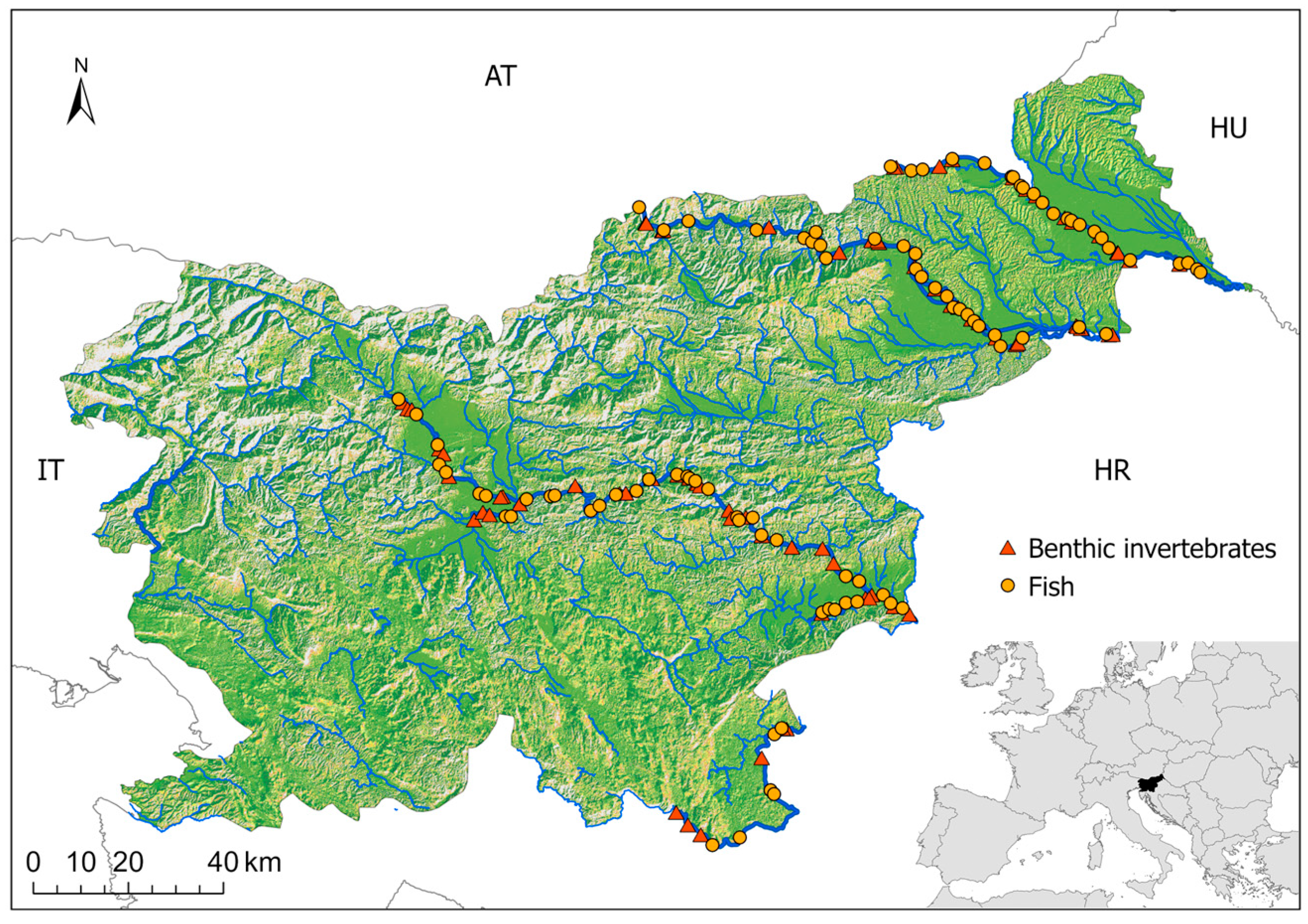
The study was conducted on large tributaries of the Danube River in Slovenia (Figure 1). All study sites are located on river sections with mean annual discharges exceeding 50 m3/s (ranging from 50.7 to 294.0 m3/s) and/or catchments larger than 2500 km2 (ranging from 1146 to 15,465 km2), and are therefore defined as large or very large rivers according to the Slovenian river typology [56,57]. The catchments of the studied rivers (that is, the Drava, Mura, Sava, Ljubljanica, Krka, and Kolpa) are characterized by a high proportion of natural land cover. Across all six river basins, natural areas dominate the landscape, accounting for approximately 65–88% of the total catchment areas, with particularly high shares in the Kolpa and Drava catchments (88% and 77%, respectively). Agricultural land use is present to a lesser extent and is mainly represented by extensive agriculture, while intensively managed agricultural areas form a comparatively smaller fraction of the catchments (minimum 3%, maximum 21%). Urban land cover is consistently low across all basins, generally not exceeding 5%. Overall, these distributions indicate a comparatively narrow catchment-scale land-use gradient across the studied rivers, particularly for intensive agriculture and urban land cover. National monitoring assessments for the studied period [58] indicated good chemical status and good or high status for the assessed general physico-chemical parameters and specific pollutants (Table S1). These assessments indicate that the studied river sections were characterized by generally good water quality and a relatively narrow water-quality gradient [39,59]. Consequently, the study sites provided a suitable environmental context for examining associations with other stressor groups, such as hydromorphological alteration and riparian land-use change, which exhibited broader gradients across the studied rivers.

2.2. Biological Data

We compiled benthic invertebrate data from 77 sampling sites and fish data from 92 sampling sites (Figure 1). Benthic invertebrates were collected from 2006 to 2013 during low water levels in spring and summer, except for the Mura and Drava rivers, which were sampled in winter due to the characteristics of their natural hydrological regimes. Samples were taken following the standardized Slovenian bioassessment protocol based on quantitative multi-habitat sampling [39,60,61]. Sampling was performed in the wadable part of the main channel or in the littoral zone of impoundments (up to 1 m depth) within a 250 m sampling site. A total of 20 subsamples were taken from microhabitat types defined as combinations of substrate and flow categories, sampled in proportion to their occurrence; microhabitats covering <5% of the site were not sampled. Each subsample was obtained by kick-sampling 0.0625 m2 of the riverbed with a hand net (0.5 mm mesh), yielding a total sampled area of 1.25 m2 per site. The 20 subsamples were pooled, and a random quarter of the composite sample was selected for laboratory processing; taxa were identified primarily to species or genus level (with some groups to (sub)family level). Fish were sampled from 2007 to 2014 during spring, summer, and early autumn by boat electrofishing using repeated “stripes” defined by the effective electric field (approximately 6 m wide and 1.5 m deep [62,63]). Before sampling, habitats in the main channel were classified as pool, riffle, or run, each occurring in either the central or lateral channel zone; these combinations were then sampled in proportion to their local coverage. Individual stripes were 50–300 m long, and each was sampled once; stripe length depended on the diversity and spatial extent of habitat types present at the site. Because the sampled areas varied among sites, fish abundance was standardized by dividing taxon counts by the total surface area of all sampled stripes. All fish were identified to the species level. In the statistical analyses, data on taxonomic composition and abundance were used.

2.3. Environmental Data

For each site, we collected data on 86 environmental variables to describe hydromorphological, land use, and typological features of the studied river sites (Table 1). Most data (e.g., hydromorphology, land use) were acquired using geographic information system (GIS) tools in ArcGIS Pro 3.2 (Esri, Redlands, CA, USA) [64]. Information for selected typological variables was obtained from previous studies and existing classifications (e.g., [56,57,65]). Hydromorphological variables were defined following the River Habitat Survey (RHS) protocol [66] and represent in-channel, bank, and riparian zone features at the local spatial scale. For a more detailed description of the data sources and procedures used to derive hydromorphological variables, including spatial processing steps, see [67]. Catchment-scale land use was quantified using the CORINE Land Cover (CLC) dataset, which provides a harmonized classification of land cover across Europe with a minimum mapping unit of 25 ha [68]. However, this minimum mapping unit was too coarse to reliably characterize small and narrow land-use features within the analyzed riparian corridors, which were 10–150 m wide. Therefore, a more detailed national land-use dataset comprising 25 land-use categories was used for the local-scale analyses. In this dataset, category-specific minimum mapping areas ranged from 0.0025 ha for urban areas and surface waters to 0.05–0.1 ha for most agricultural and riparian vegetation classes and 0.25 ha for forests [69]. Land-use categories from both datasets were aggregated into broader category groups representing dominant land-use types, namely natural cover, urban cover, intensive agriculture, and extensive agriculture. Slope and elevation variables were derived from digital elevation models (DEMs). Catchment-scale mean slope was calculated using a European-scale DEM with a spatial resolution of 25 m [70], while elevation and slope at the local scales were obtained from a higher-resolution (5 m) national DEM available for Slovenia [71]. Land use is closely linked to the input of fine sediments into river systems through soil erosion processes. Catchment-scale soil erosion rates (t ha−1 yr−1) were estimated using the PESERA dataset [72], available from the European Soil Portal, and used as a proxy for potential fine sediment delivery to river networks.

2.4. Study Design

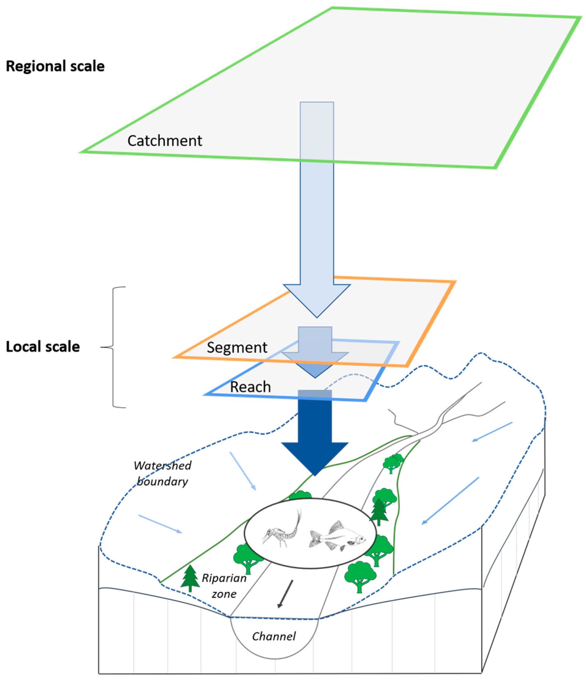
For each sampling site, data on environmental variables were obtained at two local scales (reach, segment) and one regional scale (Table 1). At the local scales, data were collected on (i) hydromorphological characteristics, (ii) riparian land use, and (iii) typological characteristics of the surveyed river sections. At the regional scale, data on typological characteristics and land use were collected at the catchment level. The environmental variables were grouped into stressor variables at three spatial scales—reach, segment, and catchment—and typological variables representing natural local and regional (catchment-scale) characteristics (Figure 2). While the catchment scale is defined by the topographic boundaries of the drainage area, the reach and segment scales were defined based on the methodological approach and results of a previous study that compared local hydromorphological and riparian land-use variables at nested river lengths of 500, 1000, 2000 and 5000 m, and riparian widths of 10, 50, 100 and 150 m [67]. The standard 500 m River Habitat Survey (RHS) length, together with the 10 and 50 m riparian widths used within the RHS framework, formed the basic spatial units. The longer nested river lengths (1000, 2000, and 5000 m) and wider riparian widths (100 and 150 m) were selected pragmatically to provide a consistent comparison across progressively larger spatial extents. In the present study, the reach scale was defined as the shortest analyzed river length of 500 m for both assemblages. In [67], the largest statistically significant increase in the explanatory contribution of hydromorphological variables for benthic invertebrates occurred between the 500 and 1000 m river lengths, whereas further increases at 2000 and 5000 m were comparatively small. We therefore selected 1000 m as a parsimonious segment-scale extent for benthic invertebrates. For fish, explanatory power increased progressively with river length, with a particularly marked and statistically significant increase between 2000 and 5000 m; consequently, 5000 m was selected as the segment-scale extent. Riparian zones were defined as 50 m-wide buffers (measured outward from the bank top) for the 500 m and 1000 m river stretches, and as 10 m-wide buffers for the 5000 m stretches. These combinations yielded the highest explanatory power of riparian land use variables for both assemblages. The present study, although based on the same biological dataset, does not repeat the scale-selection procedure or test whether these extents represent optimal spatial scales. Instead, it treats them as predefined local spatial units within a broader hierarchical framework that additionally incorporates catchment-scale stressors and natural typological variables and partitions their unique and shared contributions.

2.5. Data Preparation

Biological variables were ln(x + 1)-transformed to reduce the disproportionate influence of highly abundant taxa on the ordination results. Environmental variables were transformed using the transformation approaches presented in Table 1 to reduce skewness and the influence of extreme values on the analyses. Variables occurring in fewer than 10% of sites were excluded from the analysis. To reduce redundancy in hydromorphological data, Spearman’s rank correlation coefficients (rs) were calculated between variable pairs. In cases of |rs| > 0.8 for a variable pair, the variable with the higher overall mean correlation was discarded from further analyses (overall, 20 hydromorphological variables were discarded).

2.6. Relationships Between Regional Factors and Local Hydromorphology

Relationships between regional environmental factors and local hydromorphological variables were examined using direct gradient analyses and correlation analyses. CCA was applied to calculate simple effects (total variation explained by a variable, including both its unique and shared—correlated—components; lambda 1) and conditional effects (unique variation explained by a variable after controlling for all other variables; lambda a) of each regional variable, as well as their shared effect on overall variability in local hydromorphology (reach and segment scales). CCA was selected based on the estimation of gradient lengths (i.e., heterogeneity in response data) using Detrended Correspondence Analysis (DCA) [73]. We applied a forward-selection procedure in CANOCO 5 software (Microcomputer Power, Ithaca, NY, USA) [74]. Forward selection was used to identify a reduced subset of predictor variables, each contributing significantly (p < 0.05) to the variation in response variables [75]. The variation jointly explained by the selected variables was expressed as adjusted R2, which accounts for the number of predictors and sampling sites and reduces the overestimation associated with classical R2 [76,77,78]. To test for statistical significance of the explained variation, a Monte Carlo permutation test with 999 permutations was applied. Additionally, Spearman’s rank correlations were calculated to examine relationships between individual regional and local hydromorphological variables, using SPSS Statistics 22 software (IBM Corp., Armonk, NY, USA) [79]. The analysis was exploratory, and no correction for multiple testing was applied; consequently, the reported p-values are unadjusted.

2.7. Effects of Stressors at Three Spatial Scales and Typology on Biotic Variability in Large Rivers

Using variance partitioning, we examined the relative effects of groups of environmental variables on benthic invertebrate and fish variability. We quantified the amount of variance in biological data attributable to the unique contribution of each variable group (unique effects), as well as the variance jointly explained by overlapping effects among multiple variable groups (shared effects). This approach allows for a clear separation of unique and shared effects of pre-defined sets of predictor variables. We defined four groups of environmental variables: one group representing natural characteristics (typology) and three groups representing stressor variables acquired at the reach, segment, and catchment spatial scales. In the first step, we evaluated the relative contribution of only stressor variables acquired across the three analyzed spatial scales, without controlling for the natural environmental variability of the studied rivers. Subsequently, we assessed how accounting for this natural variability affected the interpretation of stressor impacts on the two studied biological assemblages in large rivers. To account for the influence of natural environmental variability on aquatic community structure, a typological variable group was included in the analysis alongside the stressor variable groups analyzed in the previous step.
Since CANOCO 5 limits partial gradient analyses to a maximum of three predictor groups, variance partitioning involving four groups (A, B, C, D) was performed in the following steps: (1) unique fractions were obtained by analyzing each predictor group separately while treating the variables of the remaining three groups as covariates; (2) the total explained fraction was obtained from the full model including all four predictor groups; (3) the total shared fraction was calculated as the total explained fraction minus the sum of all unique fractions; (4) pairwise shared fractions (A&B, A&C, A&D, B&C, B&D and C&D) were estimated by analyzing each pair of predictor groups while treating the remaining two groups as covariates; (5) the remaining shared fraction, representing the combined contribution of three-group and four-group overlaps, was obtained by subtracting the sum of all pairwise shared fractions from the total shared fraction. This procedure allowed the explained biological variation to be partitioned into four unique fractions, six pairwise shared fractions, and one combined shared fraction representing the overlap among three or four predictor groups.
Gradient lengths estimated using Detrended Correspondence Analysis (DCA) indicated unimodal responses for both biological datasets; therefore, partial Canonical Correspondence Analysis (pCCA) with forward selection was used [78]. To test for statistical significance of the explained variation, a Monte Carlo permutation test with 999 permutations was applied, and the “downweight rare species” option was selected to minimize the influence of rare taxa. Otherwise, the same statistical parameters and software as described in the previous section were used.

3. Results

3.1. Effects of Regional Factors on Local Hydromorphological Variability

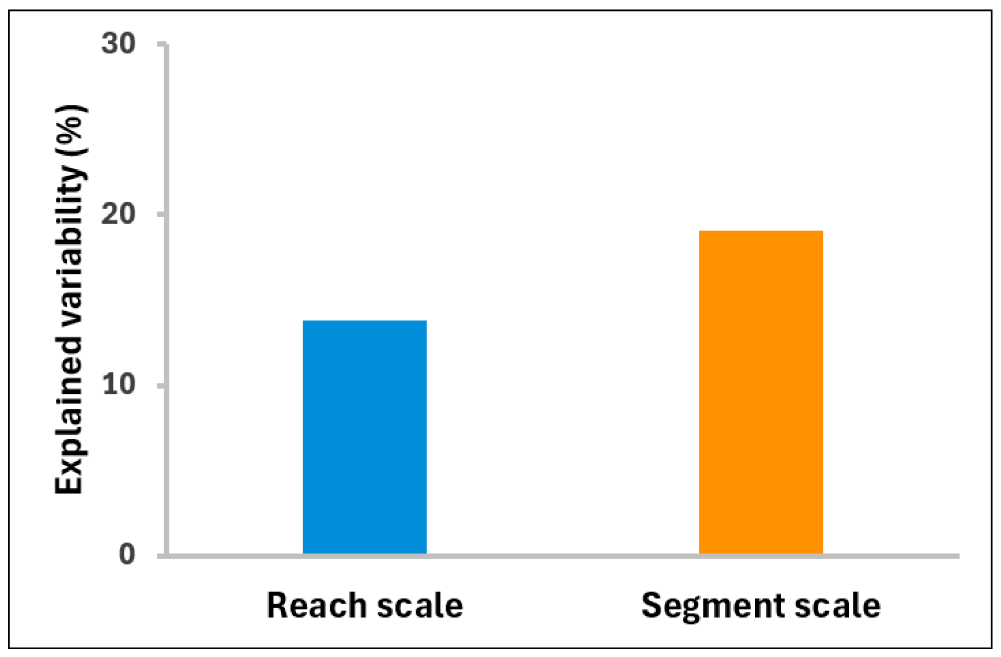
Regional environmental variables jointly explained 13.8% and 19.1% of local hydromorphological variability at the reach and segment scales, respectively (Figure 3). The same eight regional variables were retained at both scales, although they generally explained more variability at the segment scale (Table 2). Soil erosion in the catchment, an indicator of fine-sediment availability and mobility driven mainly by land cover and/or land use across the catchment, showed the highest explanatory contribution. Regarding individual hydromorphological variables (exploratory correlation analysis), we found significant correlations (unadjusted p-values < 0.05) for 26 of the total 32 hydromorphological variables analyzed (Supplementary Tables S2 and S3; given the exploratory nature of the analysis, these associations should not necessarily be interpreted as causal). Correlations involving the same hydromorphological characteristics at both spatial scales were generally stronger at the segment scale (74% of comparisons; Wilcoxon signed-rank test: Z = −8.495, p < 0.001). Ecologically interpretable patterns included positive associations of distance from source with oxbow lakes, side channels, and woody debris, reflecting the increasing complexity of downstream river sections. Average catchment slope was positively associated with the percentage of impounded river length, indicating an association between regional typology and hydropower-related modification.

3.2. Relative Effects of Local- and Regional-Scale Stressors on Aquatic Biota

Within each stressor variable group, forward selection retained five to seven variables for benthic invertebrates and five to twelve variables for fish. Each retained variable explained a significant (p < 0.05) unique fraction of assemblage variability (Table 3). The percentage of impounded river-section length was the strongest local predictor of benthic invertebrate variability (Lambda a-LR = Lambda a-LS = 6.7%), while fish variability was best explained by the percentage of reinforced bank length (Lambda a-LR = 8.0%, Lambda a-LS = 6.6%). Of the five selected catchment-scale predictors, benthic invertebrate variability was best explained by the percentage of urban land use (Lambda a = 6.8%). In contrast, fish were best explained by the percentage of intensive agriculture and percentage of natural cover (each Lambda a = 5.3%). When considering only land-use variables (analyzed in separate, spatial scale-specific CCA analyses), the catchment scale was shown to be the dominant spatial scale for explaining biotic variability, exceeding the explanatory power of both local scales for benthic invertebrates and fish. Land use at the catchment scale explained 10.4% and 6.9% of benthic invertebrate and fish variability (R2adj), respectively. In comparison, at the reach scale, land use explained 4.0% and 3.4% of benthic invertebrate and fish variability, respectively, and at the segment scale, 4.3% and 5.8%.
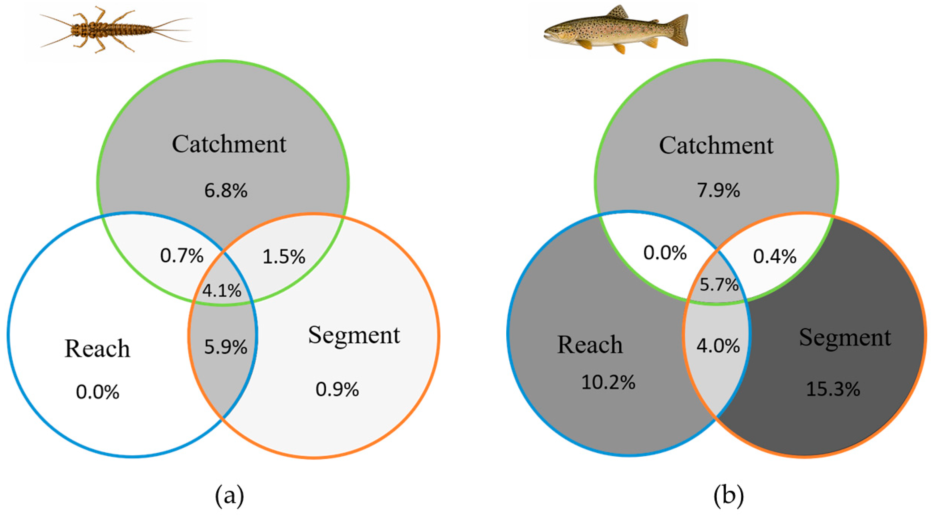
In total, stressor variables of the three analyzed spatial scales explained 43.5% (R2adj) of fish and 19.9% of benthic invertebrate variability. The largest unique contribution to explained benthic invertebrate variability was found for the catchment stressor group (R2adj = 6.8%, Figure 4a). By comparison, both local-scale stressor groups uniquely explained only a trivial fraction of benthic invertebrate variability (LS: R2adj = 0.9%) or even no variability (LR: R2adj = 0.0%). For both local-scale stressor groups, the majority of the explained variability was attributable to their shared effects (R2adj = 5.8%), indicating a substantial overlap of these predictor sets. The shared effects of each local-scale group with the catchment group were negligible, whereas the shared effects of all three stressor groups accounted for 4.1% of total benthic invertebrate variability. Overall, the combined contribution of the three stressor groups to benthic invertebrate variability was greater for shared effects (12.2%) than for unique effects (7.7%).
With respect to fish, local-scale stressor groups explained a considerably larger fraction of biotic variability compared to benthic invertebrates (Lambda a-LS = 15.3% and Lambda a-LR = 10.2%) and a notably larger fraction compared to the catchment-scale group (Lambda a = 7.9%, Figure 4b). Similar to benthic invertebrates, the shared effects of each local-scale group with the catchment group were fairly small, whereas the shared effects of all three stressor groups accounted for the largest shared effects of 5.7% total fish variability. Overall, the contribution of the three stressor groups to explained fish variability was greater for the unique effects (33.4%) than for the shared effects (10.1%).

3.3. Effects of Typology and Stressors at Local and Regional Scales on Aquatic Biota

Using a forward-selection procedure, seven typological variables were selected with significant (p < 0.05) conditional effects (Lambda a) on benthic invertebrate variability, and seven typological variables with significant conditional effects on fish variability. Among individual variables, catchment area and altitude explained the largest fractions of variability in both benthic invertebrate (6.3% and 4.4%, respectively) and fish assemblages (6.5% and 6.0%, respectively). Jointly, the selected typological variables explained 14.1% of benthic invertebrate and 18.3% of fish variability (Table 4).
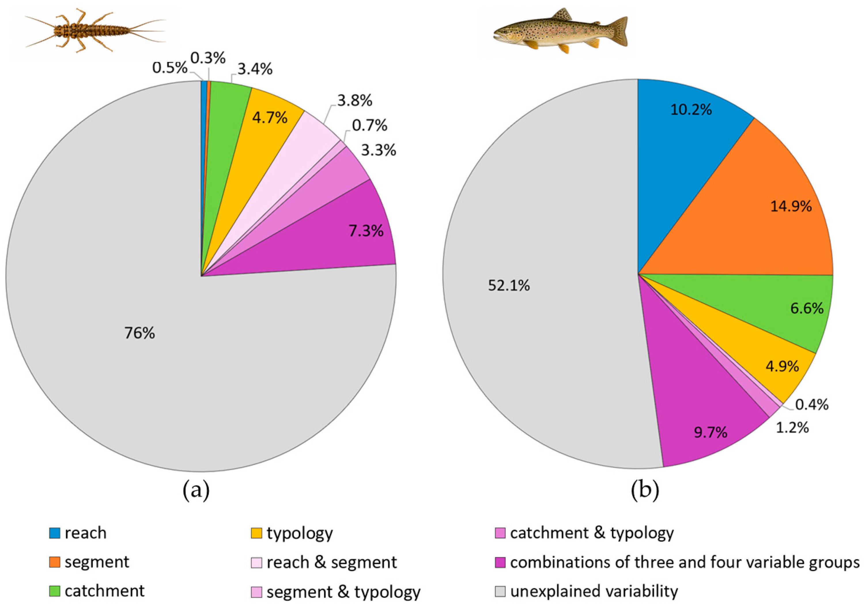
Overall, the four variable groups explained 24.0% of benthic invertebrate and 47.9% of fish variability. The largest unique fraction of benthic invertebrate variability was explained by the typology group (R2adj = 4.7%, Figure 5a), followed by the catchment stressor group (R2adj = 3.4%). An additional 3.3% of variability was explained by both of these groups (shared effects). Most benthic invertebrate variability was explained by shared effects among multiple predictor groups (63%), with the largest fraction attributable to the combined effects of three- and four-group combinations. In contrast, the largest unique fractions of fish variability were explained by both local stressor groups (R2adj-LS = 14.9%, R2adj-LR = 10.2%, Figure 5b), together accounting for roughly 52% of total explained variability. These were followed by the unique contributions of the catchment stressor group (R2adj = 6.6%) and the typology group (R2adj = 4.9%). Shared effects accounted for only about 24% of explained fish variability. Of the shared fraction, 86% was attributable to combinations of three- and four-variable groups.
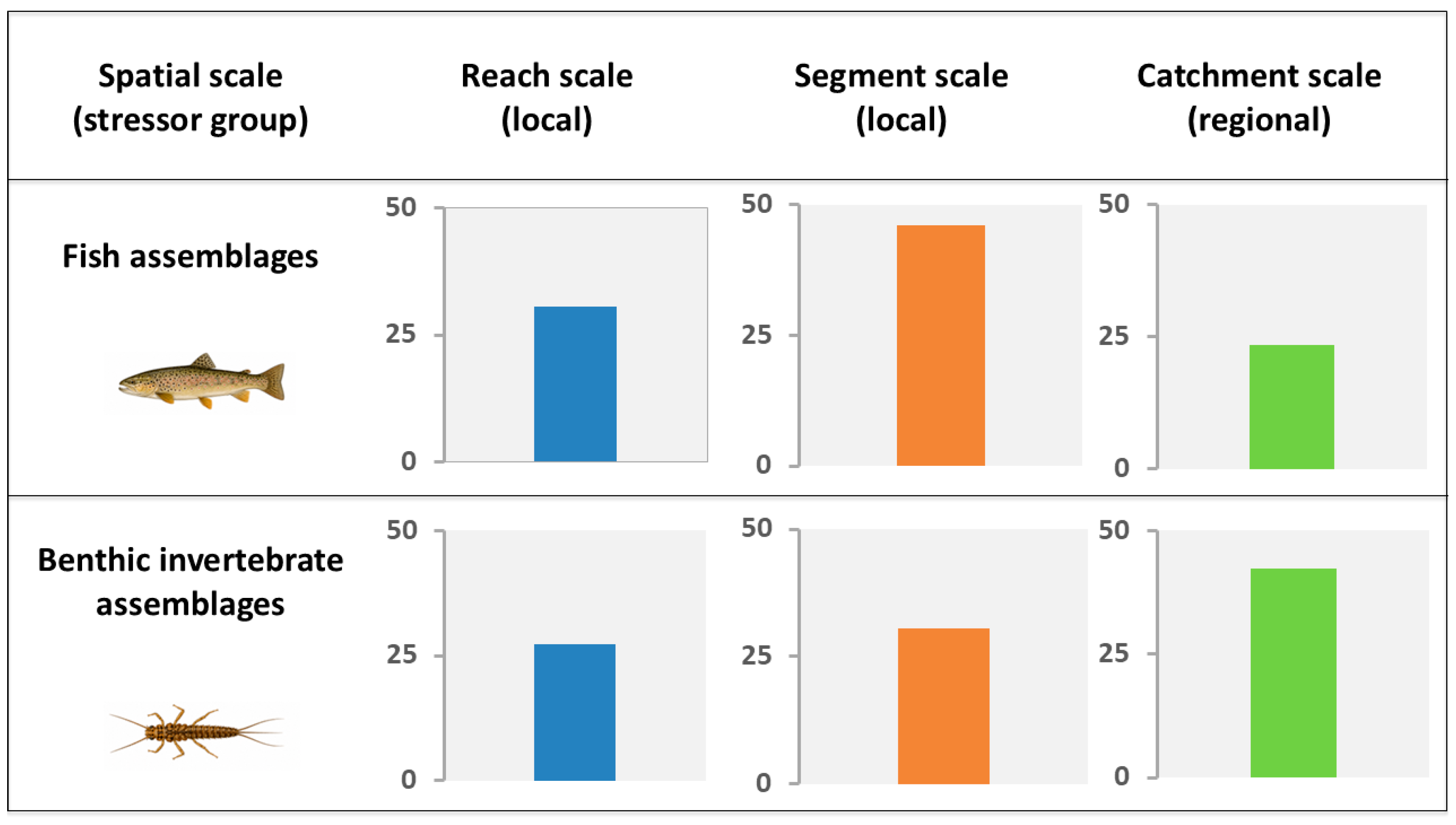
To summarize the total stressor-related contribution of each spatial scale, unique and shared fractions of the reach, segment, and catchment stressor groups were combined and expressed as relative percentages of the cumulative explained variability (Figure 6). In benthic invertebrates, the catchment scale accounted for the largest relative share of explained variability (42.4%), followed by the segment (30.4%) and reach scales (27.3%). In fish, the highest relative share was associated with the segment scale (46.0%), followed by the reach scale (30.6%), while the catchment scale accounted for 23.5% of the explained variability. This pattern indicates a clearer separation between the two local spatial scales for fish than for benthic invertebrates. It further suggests an increase in stressor importance from the local to the regional scale for benthic invertebrates, whereas no such trend is observed for fish.

4. Discussion

This study examined the scale-dependent associations of hydromorphological and land-use stressors with fish and benthic invertebrate assemblages in large, non-wadable rivers. By comparing two organism groups and partitioning unique and shared stressor effects across three spatial scales, it provides new insights for a comparatively underrepresented river category.

4.1. Relationships Between Regional and Local Environmental Variables

Many environmental factors in river landscapes covary. The hierarchical structure of river systems implies that processes operating at broader spatial scales co-shape conditions at finer scales [1]. The observed relationships among environmental variables therefore help identify potential hierarchical relationships and suggest which higher-level factors may act as indirect drivers of variation in aquatic communities.
Strong relationships between regional variables and local hydromorphological variables have been identified in several previous studies [80,81,82,83]. In this study, we found somewhat stronger correlations between regional variables and hydromorphological variables at the segment scale compared with the reach scale, which is consistent with the hierarchical model. In terms of interpretation, it is meaningful to distinguish between two types of associations: those between regional variables and hydromorphological features that reflect natural (typological) conditions and those that indicate anthropogenic modification. Regional typological factors influence not only the natural local characteristics of rivers but, through them, also the suitability of a given location for anthropogenic use [17]. In this study, regional typological variables were significantly (p < 0.05) correlated with local hydromorphological variables representing both natural and anthropogenic features. For instance, distance to source was positively correlated with typical hydromorphological characteristics of complex lowland rivers, such as oxbow lakes, large woody debris, fallen trees, and side channels. These findings indicate that, in Slovenia, the local hydromorphological characteristics of large rivers mostly still reflect conditions shaped by the expected influences of large-scale environmental factors. Similarly, the hydropower potential of a river is strongly dependent on channel slope and discharge, with steeper slopes typical of mountain streams and associated with high-energy flows [84]. In the studied large rivers, positive correlations were identified between average catchment slope (or mountain river type) and the percentage of impounded river length. We also found that riverbanks of large mountain rivers are more frequently modified than those of large lowland rivers, where anthropogenic use is often somewhat distanced from the direct impact of floodplain flooding. Some observed correlations are more difficult to interpret in terms of causality; e.g., correlations between catchment-scale land use and local bank vegetation complexity, bedrock occurrence, or mid-channel bar formation. Such patterns demonstrate that not all statistically significant correlations represent ecologically meaningful associations and must therefore be interpreted with caution; they may be random or exhibit parallel responses to other drivers not accounted for in this study.

4.2. Biological Responses to Local and Regional Stressors and Typology

In this study, the analyzed local and regional environmental variables explained nearly half of the total variability in fish and roughly one-quarter of the total variability in benthic invertebrates. The lower fraction explained for benthic invertebrates was expected and has been reported previously (e.g., [8]). Challenges associated with benthic invertebrates include high taxonomic heterogeneity, differences in taxonomic resolution applied during identification, and methodological constraints related to sampling in large rivers [15,16,85]. Because fish were identified to species level, whereas some benthic invertebrate groups were identified at higher taxonomic levels, species with different ecological preferences may have been grouped within the same taxonomic unit. This may have masked species-specific responses and should be considered when directly comparing the explained variability of the two assemblages. Additionally, the omission of characteristics at finer spatial scales such as substrate composition and other microhabitat features, which have been reported to be critical determinants of benthic invertebrate structure [10,59], may have contributed to the low explained variance found in this study. Because such variables are typically difficult to quantify at sufficiently fine spatial resolutions using GIS-based approaches, future analyses should complement GIS-based methods with field survey data [86]. An additional explanation may be the relatively narrow gradient of water pollution included in this study. Numerous previous studies have identified water pollution, rather than hydromorphological alterations or land use, as the primary driver shaping benthic invertebrates in rivers ([4,7,8,9], but see [87]). Nevertheless, our results confirmed that both aquatic assemblages integrate environmental effects across spatial scales, albeit with different relative contributions, and respond to the combined influence of multiple, often interdependent environmental variables rather than to isolated variables acting at a single scale. Considering stressors only, the three stressor groups explained 43.5% of fish variability, substantially more than the 19.9% explained for benthic invertebrates. The explained variability of benthic invertebrate assemblages was relatively evenly partitioned among unique effects of catchment-scale stressors, unique effects of local stressors, and their shared effects (not supporting the benthic-invertebrate prediction in H2). Notably, a significant proportion of local-stressor effects could not be clearly distinguished between the reach and segment scales (i.e., a high shared effect), likely due to the limited spatial differentiation between the two scales defined for benthic invertebrates (500 m and 1000 m). In contrast, fish assemblages were characterized by a substantially larger proportion of explained variability attributable to local-scale stressors (also reported [8,41,88,89,90,91]), accounting for approximately two-thirds of the total explained variability, while catchment-scale stressors and the shared effects of regional and local stressors contributed considerably less. Notably, the largest share of explained fish variability was associated with stressors operating at the segment scale (supporting the fish-related prediction in H2). The importance of the segment scale for fish has been recognized in previous studies and is linked to their habitat requirements, which are generally fulfilled at larger spatial scales [55,67]. For both assemblages, the pairwise shared fraction between the reach- and segment-scale groups exceeded those between either the local-scale group and the catchment-scale group (supporting H3).
With the inclusion of the typological variable group, the overall pattern regarding the relative importance of individual stressor groups (in terms of their unique and shared effects) did not change substantially. The unique contribution of the typology group to both benthic invertebrate and fish assemblages was comparable and explained a relatively small fraction of total biotic variability (slightly below 5% in both cases; broadly supporting H4). For benthic invertebrates, however, this represented the largest single unique fraction of explained variability, indicating that natural factors still dominated over hydromorphological stressors. In contrast to fish, benthic invertebrates also exhibited a modest increase in the proportion of shared effects when typological variables were included, indicating a stronger interdependence between natural typological gradients and stressor-related variables. Among individual typological variables, catchment size was found to be most important for explaining both fish and benthic invertebrate communities, which is consistent with results of previous studies (e.g., [92,93,94]).
At the local scale, hydromorphological variables were more important compared to land-use variables for explaining the variability of both aquatic assemblages. However, these results should be interpreted with caution, as both groups of variables partly cover the same physical space—the riparian corridor—and may at least partially capture the same anthropogenic change or driver. For example, a driver such as flood protection induces changes typically classified as hydromorphological pressures (e.g., levee construction or bank reinforcement), while often simultaneously resulting in altered riparian land cover through vegetation removal or reduced natural cover. Conversely, drivers associated with land-use change, such as urban development or agricultural expansion, may lead to loss of key riparian habitats or morphological features (e.g., through the infilling of oxbow lakes or drainage of side channels). They may also trigger physical (i.e., hydromorphological) modifications of riparian zones to protect newly established land uses, for example, through bank reinforcement to restrict lateral channel migration or channel deepening and narrowing to reduce flood risk. Thus, the same anthropogenic modification may be captured by two or more stressor variables methodologically classified into separate stressor groups, which may lead to misinterpretation of statistical outcomes. Multivariate statistical approaches such as forward selection attribute overlapping explained variability to the predictor with greater overall explanatory power. However, this statistical attribution does not necessarily identify the underlying causal driver. In this context, the spatial scale at which pressures operate may represent a more informative management guide than the stressor category itself, provided that the primary underlying driver is identified before implementation of management measures. Effective river management should therefore prioritize the identification of dominant drivers at the relevant spatial scale, rather than focusing exclusively on the formal classification of pressures.
Land use at the catchment scale explained larger fractions of benthic invertebrate and fish variability than local-scale land use (contrary to H1), with the difference between regional and local scales being more pronounced for benthic invertebrates than for fish. Regarding benthic invertebrates, our results are in line with various previous studies that also found greater importance of catchment-scale than local-scale land use [13,40,95]. One explanation may be the large size of the studied rivers, as the cumulative effects of land use operating across extensive catchments can outweigh the influence of riparian land use [96]. Differences among individual land-use categories were not substantial, but slightly higher fractions of explained variability were associated with urban cover and intensive agriculture. Compared to the other analyzed predictor groups, catchment-scale land use contributed relatively small unique fractions of explained biotic variability, accounting for roughly 14% for both benthic invertebrate and fish assemblages (an additional ~14% of benthic invertebrate variability was explained by the shared effects of catchment-scale land use and typological variables). A possible explanation for this comparatively modest contribution of catchment land use is the relatively narrow land-use gradient observed across the studied rivers. Catchments of the studied large Slovenian rivers are dominated by natural land cover (ranging from 64% to 91%, and averaging 75%). In comparison, urban areas and intensive agriculture occupy only smaller percentages (with maximums of 5% and 22%, respectively). Previous studies have demonstrated that the detection and magnitude of biological responses to land-use change strongly depend on the range of the land-use gradient considered, with studies conducted across more homogeneous landscapes often reporting weaker or non-detectable responses of aquatic communities (e.g., [40,97,98,99]). Ecological responses may only become detectable once certain thresholds of land-use conversion are exceeded—for example, a minimum of 50% [24]—highlighting the importance of sufficiently broad land-use gradients for capturing landscape-driven effects on riverine biota. This interpretation is linked to the consistently good to very good physico-chemical status recorded across the study sites, indicating that catchment land use did not translate into substantial physico-chemical pressures. Given that catchment-scale land use often influences aquatic communities indirectly through its effects on water chemistry [6], the absence of pronounced physico-chemical degradation may partly explain the relatively weak biological responses to land-use variables observed in this study. Compared with the catchment scale, land use at the local scale (across the analyzed riparian buffers) exhibited wider gradients (see Table 1). The highest percentage of natural cover was observed within the narrowest 10 m buffer (77%). Although natural cover declined with increasing buffer width, from 50% in the 50 m buffer to 46% in the 100 m buffer and 43% in the 150 m buffer, it remained the dominant land-use category.

5. Study Limitations

This study has some limitations that should be acknowledged. First, the analyses were based on environmental data collected with GIS-based approaches, which still cannot fully replace field-based measurements; consequently, some variables were simplified or not available (e.g., substrate type). Second, although variance partitioning enabled the separation of unique and shared effects of stressor groups, a substantial proportion of explained variability was attributed to shared fractions among predictors. This reflects their interdependence, which may partly arise from hierarchical relationships among spatial scales but also from non-causal correlations that obscure the identification of the underlying drivers and limit the interpretability of individual effects. Third, formal residual spatial autocorrelation was not assessed. Although the typological variables may capture part of the broad-scale spatially structured environmental variation, they do not provide an explicit spatial correction. Some residual spatial dependence may therefore remain and may have influenced the estimated fractions of explained variability. Fourth, the study focused exclusively on large rivers in Slovenia, and the findings are therefore context-dependent; extrapolation to other river types or regions with different environmental settings should be made with caution. Fifth, biological sampling in non-wadable rivers is methodologically challenging. Deeper mid-channel habitats, which often represent an important share of habitat diversity, remain inaccessible and therefore unsampled. As a result, the collected assemblages may not fully reflect the overall community structure present at a sampling site. Finally, benthic invertebrate and fish samples were collected from largely overlapping river sections and periods. However, sampling was not systematically matched by site location and sampling date, which may have influenced the analytical results.

6. Conclusions

The multi-scale analysis conducted in this study suggests that restoration planning may benefit from aligning management actions with organism-specific associations rather than applying interventions at a uniform spatial scale. Benthic invertebrates were primarily associated with combined cross-scale effects, suggesting potential benefits of integrating catchment-scale reduction of diffuse pressures with coordinated local habitat improvements. In contrast, fish assemblages showed clearer associations with local stressors, suggesting that segment-scale interventions may warrant priority. These results highlight the value of identifying relevant environmental factors at appropriate spatial scales. From a sustainability perspective, such scale-matched approaches may help improve the efficiency of restoration measures, enhance ecological resilience, and support long-term improvements in ecological status by reducing potential mismatches between pressures and interventions. However, the specific management implications presented here should be interpreted primarily in the context of large non-wadable rivers with similar environmental conditions. Intervention-based studies, such as before–after restoration studies, which have not yet been conducted on the studied rivers, will be needed to reliably evaluate the effectiveness of specific restoration measures.

Supplementary Materials

The following supporting information can be downloaded at: https://www.mdpi.com/article/10.3390/su18178613/s1, Table S1: Water Framework Directive status classes for selected general physico-chemical quality elements (BOD5, nitrate and total phosphorus), and specific pollutants in water bodies encompassing the studied river sections (period 2009–2013); Table S2: Statistically significant (p < 0.05) correlations (Spearman’s rho) between regional variables and local hydromorphological variables at the reach scale; Table S3: Statistically significant (p < 0.05) correlations (Spearman’s rho) between regional variables and local hydromorphological variables at the segment scale.

Author Contributions

Conceptualization, M.K. and G.U.; methodology, M.K. and G.U.; software, M.K.; validation, M.K. and G.U.; formal analysis, M.K.; investigation, M.K. and G.U.; resources, M.K. and G.U.; data curation, M.K. and G.U.; writing—original draft preparation, M.K.; writing—review and editing, M.K. and G.U.; visualization, M.K. and G.U.; supervision, G.U.; project administration, G.U.; funding acquisition, G.U. All authors have read and agreed to the published version of the manuscript.

Funding

This research was supported by the Slovenian Research and Innovation Agency (ARIS), and the Ministry of the Environment and Spatial Planning of the Republic of Slovenia, partially through the research project “Hydromorphological Typology of Rivers in Slovenia” (“Target Research Program (CRP) 2024”, project no. V2-24034).

Institutional Review Board Statement

Not applicable.

Informed Consent Statement

Not applicable.

Data Availability Statement

The data presented in this study are available on request from the corresponding author.

Acknowledgments

We gratefully acknowledge Samo Podgornik for compiling and organizing the fish dataset.

Conflicts of Interest

The authors declare no conflicts of interest.

References

  1. Frissell, C.A.; Liss, W.J.; Warren, C.E.; Hurley, M.D. A Hierarchical Framework for Stream Habitat Classification: Viewing Streams in a Watershed Context. Environ. Manag. 1986, 10, 199–214. [Google Scholar] [CrossRef] [Scilit]
  2. Hawkins, C.P.; Kershner, J.L.; Bisson, P.A.; Bryant, M.D.; Decker, L.M.; Gregory, S.V.; McCullough, D.A.; Overton, C.K.; Reeves, G.H.; Steedman, R.J.; et al. A Hierarchical Approach to Classifying Stream Habitat Features. Fisheries 1993, 18, 3–12. [Google Scholar] [CrossRef] [Scilit]
  3. Poff, N.L. Landscape Filters and Species Traits: Towards Mechanistic Understanding and Prediction in Stream Ecology. J. N. Am. Benthol. Soc. 1997, 16, 391–409. [Google Scholar] [CrossRef] [Scilit]
  4. Hering, D.; Johnson, R.K.; Kramm, S.; Schmutz, S.; Szoszkiewicz, K.; Verdonschot, P.F.M. Assessment of European Streams with Diatoms, Macrophytes, Macroinvertebrates and Fish: A Comparative Metric-Based Analysis of Organism Response to Stress. Freshw. Biol. 2006, 51, 1757–1785. [Google Scholar] [CrossRef] [Scilit]
  5. Johnson, R.K.; Hering, D.; Furse, M.T.; Clarke, R.T. Detection of Ecological Change Using Multiple Organism Groups: Metrics and Uncertainty. Hydrobiologia 2006, 566, 115–137. [Google Scholar] [CrossRef] [Scilit]
  6. Flinders, C.A.; Horwitz, R.J.; Belton, T. Relationship of Fish and Macroinvertebrate Communities in the Mid-Atlantic Uplands: Implications for Integrated Assessments. Ecol. Indic. 2008, 8, 588–598. [Google Scholar] [CrossRef] [Scilit]
  7. Johnson, R.K.; Hering, D. Response of Taxonomic Groups in Streams to Gradients in Resource and Habitat Characteristics. J. Appl. Ecol. 2009, 46, 175–186. [Google Scholar] [CrossRef] [Scilit]
  8. Marzin, A.; Verdonschot, P.F.M.; Pont, D. The Relative Influence of Catchment, Riparian Corridor, and Reach-Scale Anthropogenic Pressures on Fish and Macroinvertebrate Assemblages in French Rivers. Hydrobiologia 2013, 704, 375–388. [Google Scholar] [CrossRef] [Scilit]
  9. Dahm, V.; Hering, D.; Nemitz, D.; Graf, W.; Schmidt-Kloiber, A.; Leitner, P.; Melcher, A.; Feld, C.K. Effects of Physico-Chemistry, Land Use and Hydromorphology on Three Riverine Organism Groups: A Comparative Analysis with Monitoring Data from Germany and Austria. Hydrobiologia 2013, 704, 389–415. [Google Scholar] [CrossRef] [Scilit]
  10. Villeneuve, B.; Piffady, J.; Valette, L.; Souchon, Y.; Usseglio-Polatera, P. Direct and Indirect Effects of Multiple Stressors on Stream Invertebrates across Watershed, Reach and Site Scales: A Structural Equation Modelling Better Informing on Hydromorphological Impacts. Sci. Total Environ. 2018, 612, 660–671. [Google Scholar] [CrossRef] [Scilit] [PubMed]
  11. Birk, S.; Chapman, D.; Carvalho, L.; Spears, B.M.; Andersen, H.E.; Argillier, C.; Auer, S.; Baattrup-Pedersen, A.; Banin, L.; Beklioğlu, M.; et al. Impacts of Multiple Stressors on Freshwater Biota across Spatial Scales and Ecosystems. Nat. Ecol. Evol. 2020, 4, 1060–1068. [Google Scholar] [CrossRef] [Scilit] [PubMed]
  12. Feld, C.K. Response of Three Lotic Assemblages to Riparian and Catchment-Scale Land Use: Implications for Designing Catchment Monitoring Programmes. Freshw. Biol. 2013, 58, 715–729. [Google Scholar] [CrossRef] [Scilit]
  13. Leps, M.; Tonkin, J.D.; Dahm, V.; Haase, P.; Sundermann, A. Disentangling Environmental Drivers of Benthic Invertebrate Assemblages: The Role of Spatial Scale and Riverscape Heterogeneity in a Multiple Stressor Environment. Sci. Total Environ. 2015, 536, 546–556. [Google Scholar] [CrossRef] [Scilit] [PubMed]
  14. Bayley, P.B. Understanding Large River: Floodplain Ecosystems. BioScience 1995, 45, 153–158. [Google Scholar] [CrossRef] [Scilit] [PubMed]
  15. Blocksom, K.A.; Flotemersch, J.E. Comparison of Macroinvertebrate Sampling Methods for Nonwadeable Streams. Environ. Monit. Assess. 2005, 102, 243–262. [Google Scholar] [CrossRef] [Scilit] [PubMed]
  16. Jones, J.I.; Davy-Bowker, J. Standardisation of RIVPACS for Deep Rivers: Phase I—Review of Techniques for Sampling Benthic Macro-Invertebrates in Deep Rivers; Freshwater Biological Association, The River Laboratory: Wareham, UK, 2014; p. 58. [Google Scholar]
  17. Allan, J.D. Landscapes and Riverscapes: The Influence of Land Use on Stream Ecosystems. Annu. Rev. Ecol. Evol. Syst. 2004, 35, 257–284. [Google Scholar] [CrossRef] [Scilit]
  18. Begon, M.; Townsend, C.R. Ecology: From Individuals to Ecosystems, 5th ed.; Wiley: Hoboken, NJ, USA; Chichester, UK, 2021; ISBN 978-1-119-27935-8. [Google Scholar]
  19. Lange, K.; Townsend, C.R.; Matthaei, C.D. Can Biological Traits of Stream Invertebrates Help Disentangle the Effects of Multiple Stressors in an Agricultural Catchment? Freshw. Biol. 2014, 59, 2431–2446. [Google Scholar] [CrossRef] [Scilit]
  20. Schinegger, R.; Palt, M.; Segurado, P.; Schmutz, S. Untangling the Effects of Multiple Human Stressors and Their Impacts on Fish Assemblages in European Running Waters. Sci. Total Environ. 2016, 573, 1079–1088. [Google Scholar] [CrossRef] [Scilit] [PubMed]
  21. Bao, S.; Heino, J.; Xiong, H.; Wang, J. Disentangling the Effects of Multiple Stressors on Freshwater Macroinvertebrates: A Quantitative Analysis of Experimental Studies. Ecol. Indic. 2024, 169, 112880. [Google Scholar] [CrossRef] [Scilit]
  22. Carmichael, H.; Warfield, R.; Yvon-Durocher, G. Reconciling Variability in Multiple Stressor Effects Using Environmental Performance Curves. Ecol. Lett. 2025, 28, e70065. [Google Scholar] [CrossRef] [Scilit] [PubMed]
  23. Chen, K.; Midway, S.R.; Peoples, B.K.; Wang, B.; Olden, J.D. Shifting Taxonomic and Functional Community Composition of Rivers under Land Use Change. Ecology 2023, 104, e4155. [Google Scholar] [CrossRef] [Scilit] [PubMed]
  24. Camana, M.; Ortega, J.C.G.; Brejão, G.L.; Melo, A.S.; Dias, M.S.; Becker, F.G. A Global Meta-Analysis of the Effects of Land Use on the Diversity of Stream Fish and Macroinvertebrates. Aquat. Sci. 2024, 86, 86. [Google Scholar] [CrossRef] [Scilit]
  25. Moss, B. Ecology of Freshwaters: A View for the Twenty-First Century, 4th ed.; 1. publ.; Wiley-Blackwell: Chichester, UK, 2010; ISBN 978-1-4443-3474-6. [Google Scholar]
  26. Resh, V.H.; Brown, A.V.; Covich, A.P.; Gurtz, M.E.; Li, H.W.; Minshall, G.W.; Reice, S.R.; Sheldon, A.L.; Wallace, J.B.; Wissmar, R.C. The Role of Disturbance in Stream Ecology. J. N. Am. Benthol. Soc. 1988, 7, 433–455. [Google Scholar] [CrossRef] [Scilit]
  27. Elosegi, A.; Díez, J.; Mutz, M. Effects of Hydromorphological Integrity on Biodiversity and Functioning of River Ecosystems. Hydrobiologia 2010, 657, 199–215. [Google Scholar] [CrossRef] [Scilit]
  28. Hohensinner, S.; Hauer, C.; Muhar, S. River Morphology, Channelization, and Habitat Restoration. In Riverine Ecosystem Management; Schmutz, S., Sendzimir, J., Eds.; Springer International Publishing: Cham, Switzerland, 2018; pp. 41–65. ISBN 978-3-319-73249-7. [Google Scholar]
  29. Winterbottom, S.J. Medium and Short-Term Channel Planform Changes on the Rivers Tay and Tummel, Scotland. Geomorphology 2000, 34, 195–208. [Google Scholar] [CrossRef] [Scilit]
  30. Rinaldi, M. Recent Channel Adjustments in Alluvial Rivers of Tuscany, Central Italy. Earth Surf. Process. Landf. 2003, 28, 587–608. [Google Scholar] [CrossRef] [Scilit]
  31. Dewson, Z.S.; James, A.B.W.; Death, R.G. A Review of the Consequences of Decreased Flow for Instream Habitat and Macroinvertebrates. J. N. Am. Benthol. Soc. 2007, 26, 401–415. [Google Scholar] [CrossRef] [Scilit]
  32. Gurnell, A. Plants as River System Engineers. Earth Surf. Process. Landf. 2014, 39, 4–25. [Google Scholar] [CrossRef] [Scilit]
  33. Junk, W.J.; Bayley, P.B.; Sparks, R.E. The Flood-Pulse Concept in River-Floodplain Systems; Canadian Special Publication in Fisheries and Aquatic Sciences: Ottawa, ON, Canada, 1989; pp. 110–127. [Google Scholar]
  34. Tockner, K.; Robinson, C.T.; Uehlinger, U. Rivers of Europe, 1st ed.; Academic Press: Oxford, UK, 2006; p. 728. [Google Scholar]
  35. Nilsson, C.; Reidy, C.A.; Dynesius, M.; Revenga, C. Fragmentation and Flow Regulation of the World’s Large River Systems. Science 2005, 308, 405–408. [Google Scholar] [CrossRef] [Scilit] [PubMed]
  36. Erős, T.; Tóth, B.; Sevcsik, A.; Schmera, D. Comparison of Fish Assemblage Diversity in Natural and Artificial Rip-Rap Habitats in the Littoral Zone of a Large River (River Danube, Hungary). Int. Rev. Hydrobiol. 2008, 93, 88–105. [Google Scholar] [CrossRef] [Scilit]
  37. Mérigoux, S.; Lamouroux, N.; Olivier, J.; Dolédec, S. Invertebrate Hydraulic Preferences and Predicted Impacts of Changes in Discharge in a Large River. Freshw. Biol. 2009, 54, 1343–1356. [Google Scholar] [CrossRef] [Scilit]
  38. Blettler, M.C.M.; Amsler, M.L.; Ezcurra De Drago, I.; Drago, E.C.; Paira, A.R.; Espinola, L.A. Hydrodynamic and Morphologic Effects on the Benthic Invertebrate Ecology along a Meander Bend of a Large River (Paraguay River, Argentina–Paraguay). Ecol. Eng. 2012, 44, 233–243. [Google Scholar] [CrossRef] [Scilit]
  39. Urbanič, G. Hydromorphological Degradation Impact on Benthic Invertebrates in Large Rivers in Slovenia. Hydrobiologia 2014, 729, 191–207. [Google Scholar] [CrossRef] [Scilit]
  40. Death, R.G.; Collier, K.J. Measuring Stream Macroinvertebrate Responses to Gradients of Vegetation Cover: When Is Enough Enough? Freshw. Biol. 2010, 55, 1447–1464. [Google Scholar] [CrossRef] [Scilit]
  41. Wang, L.; Lyons, J.; Kanehl, P. Impacts of Urban Land Cover on Trout Streams in Wisconsin and Minnesota. Trans. Am. Fish. Soc. 2003, 132, 825–839. [Google Scholar] [CrossRef] [Scilit]
  42. Niyogi, D.K.; Koren, M.; Arbuckle, C.J.; Townsend, C.R. Stream Communities Along a Catchment Land-Use Gradient: Subsidy-Stress Responses to Pastoral Development. Environ. Manag. 2007, 39, 213–225. [Google Scholar] [CrossRef] [Scilit] [PubMed]
  43. Petsch, D.K.; Blowes, S.A.; Melo, A.S.; Chase, J.M. A Synthesis of Land Use Impacts on Stream Biodiversity across Metrics and Scales. Ecology 2021, 102, e03498. [Google Scholar] [CrossRef] [Scilit] [PubMed]
  44. Wood, P.J. Biological Effects of Fine Sediment in the Lotic Environment. Environ. Manag. 1997, 21, 203–217. [Google Scholar] [CrossRef] [Scilit] [PubMed]
  45. Fohrer, N.; Haverkamp, S.; Eckhardt, K.; Frede, H.-G. Hydrologic Response to Land Use Changes on the Catchment Scale. Phys. Chem. Earth Part B Hydrol. Oceans Atmos. 2001, 26, 577–582. [Google Scholar] [CrossRef] [Scilit]
  46. Walsh, C.J.; Roy, A.H.; Feminella, J.W.; Cottingham, P.D.; Groffman, P.M.; Morgan, R.P. The Urban Stream Syndrome: Current Knowledge and the Search for a Cure. J. N. Am. Benthol. Soc. 2005, 24, 706–723. [Google Scholar] [CrossRef]
  47. Johnson, R.K.; Angeler, D.G. Effects of Agricultural Land Use on Stream Assemblages: Taxon-Specific Responses of Alpha and Beta Diversity. Ecol. Indic. 2014, 45, 386–393. [Google Scholar] [CrossRef] [Scilit]
  48. European Environment Agency. Europe’s State of Water 2024: The Need for Improved Water Resilience; Publications Office of the European Union: Luxembourg, 2024. [Google Scholar]
  49. Roni, P.; Hanson, K.; Beechie, T. Global Review of the Physical and Biological Effectiveness of Stream Habitat Rehabilitation Techniques. N. Am. J. Fish. Manag. 2008, 28, 856–890. [Google Scholar] [CrossRef] [Scilit]
  50. Rubin, Z.; Kondolf, G.; Rios-Touma, B. Evaluating Stream Restoration Projects: What Do We Learn from Monitoring? Water 2017, 9, 174. [Google Scholar] [CrossRef] [Scilit]
  51. Roni, P.; Hall, J.E.; Drenner, S.M.; Arterburn, D. Monitoring the Effectiveness of Floodplain Habitat Restoration: A Review of Methods and Recommendations for Future Monitoring. WIREs Water 2019, 6, e1355. [Google Scholar] [CrossRef] [Scilit]
  52. Stoffers, T.; Buijse, A.D.; Geerling, G.W.; Jans, L.H.; Schoor, M.M.; Poos, J.J.; Verreth, J.A.J.; Nagelkerke, L.A.J. Freshwater Fish Biodiversity Restoration in Floodplain Rivers Requires Connectivity and Habitat Heterogeneity at Multiple Spatial Scales. Sci. Total Environ. 2022, 838, 156509. [Google Scholar] [CrossRef] [Scilit] [PubMed]
  53. Kail, J.; Hering, D. The Influence of Adjacent Stream Reaches on the Local Ecological Status of Central European Mountain Streams. River Res. Appl. 2009, 25, 537–550. [Google Scholar] [CrossRef] [Scilit]
  54. Angermeier, P.L.; Winston, M.R. Local vs. Regional Influences on Local Diversity in Stream Fish Communities of Virginia. Ecology 1998, 79, 911–927. [Google Scholar] [CrossRef]
  55. Haase, P.; Hering, D.; Jähnig, S.C.; Lorenz, A.W.; Sundermann, A. The Impact of Hydromorphological Restoration on River Ecological Status: A Comparison of Fish, Benthic Invertebrates, and Macrophytes. Hydrobiologia 2013, 704, 475–488. [Google Scholar] [CrossRef] [Scilit]
  56. Urbanič, G. Inland Water Subecoregions and Bioregions of Slovenia. Nat. Slov. 2008, 10, 5–19. [Google Scholar]
  57. Urbanič, G. Ecological Status Assessment of the Rivers in Slovenia—An Overview. Nat. Slov. 2011, 13, 5–16. [Google Scholar] [CrossRef] [Scilit]
  58. Stanje Površinskih Voda. Agencija Republike Slovenije za Okolje (ARSO). Available online: https://www.gov.si/teme/stanje-povrsinskih-voda/ (accessed on 1 December 2025).
  59. Urbanič, G.; Mihaljević, Z.; Petkovska, V.; Pavlin Urbanič, M. Back to Ecology: Reference Conditions as a Basis for Assessment, Restoration and Sustainable Management of Large Rivers. Water 2021, 13, 2596. [Google Scholar] [CrossRef] [Scilit]
  60. Urbanič, G.; Tavzes, B.; Toman, M.J.; Ambrožič, Š.; Hodnik, V.; Zdešar, K.; Sever, M. Priprava Metodologij Vzorčenja Ter Laboratorijske Obdelave Vzorcev Bentoških Nevretenčarjev (Zoobentosa) Nabranih v Vodotokih in Obdelava 70 Vzorcev Bentoških Nevretenčarjev; Biotehniška Fakulteta: Ljubljana, Slovenia, 2005; p. 38. [Google Scholar]
  61. Ministrstvo za Okolje in Prostor. Pravilnik o Monitoringu Stanja Površinskih Voda. Off. Gaz. Repub. Slov. 2009, 10, 832–839. [Google Scholar]
  62. Schmutz, S.; Zauner, G.; Eberstaller, J.; Jungwirth, M. Die Streifenbefischungsmethode: Eine Methode zur Quantifizierung von Fischbeständen mittelgroßer Fließgewässer. Osterr. Fisch. 2001, 54, 14–27. [Google Scholar]
  63. Podgornik, S.; Urbanič, G. Vrednotenje Ekološkega Stanja Velikih Rek Na Podlagi Rib; Zavod za ribištvo Slovenije: Spodnje Gameljne, Slovenia, 2015; p. 91. [Google Scholar]
  64. ESRI. ArcGIS Desktop; Environmental Systems Research Institute: Redlands, CA, USA, 2014. [Google Scholar]
  65. Urbanič, G. Redelineation of European Inland Water Ecoregions in Slovenia. Rev. Hydrobiol. 2008, 1, 17–25. [Google Scholar]
  66. Raven, P.J.; Holmes, N.T.H.; Dawson, F.H.; Fox, P.J.A.; Everard, M.; Fozzard, I.R.; Rouen, K.J. River Habitat Survey in Britain and Ireland; Environment Agency: Rotterdam, The Netherlands, 2003; p. 74.
  67. Knehtl, M.; Podgornik, S.; Urbanič, G. Scale-Depended Effects of Hydromorphology and Riparian Land-Use on Benthic Invertebrates and Fish: Implications for Large River Management. Hydrobiologia 2021, 848, 3447–3467. [Google Scholar] [CrossRef] [Scilit]
  68. Copernicus Land Monitoring Service. Corine Land Cover (CLC). Available online: https://sdi.eea.europa.eu/catalogue/srv/api/records/916c0ee7-9711-4996-9876-95ea45ce1d27 (accessed on 5 May 2024).
  69. Ministry of Agriculture, Forestry and Food (MKGP) Portal. Available online: http://rkg.gov.si/GERK/ (accessed on 4 February 2023).
  70. Digital Elevation Model over Europe (EU-DEM). European Environment Agency (EEA). Available online: https://www.eea.europa.eu/data-and-maps/data/eu-dem (accessed on 3 November 2023).
  71. Ministrstvo za Okolje in Prostor—Portal Prostor. Geodetska Uprava Republike Slovenija (GURS). Available online: https://www.e-prostor.gov.si/ (accessed on 7 May 2023).
  72. Pan-European Soil Erosion Risk Assessment (PESERA). European Soil Data Centre (ESDAC). Available online: https://esdac.jrc.ec.europa.eu/content/pan-european-soil-erosion-risk-assessment-pesera (accessed on 25 April 2022).
  73. Hill, M.O.; Gauch, H.G. Detrended Correspondence Analysis: An Improved Ordination Technique. Vegetatio 1980, 42, 47–58. [Google Scholar] [CrossRef] [Scilit]
  74. ter Braak, C.J.F.; Šmilauer, P. Canoco Reference Manual and User’s Guide: Software for Ordination (Version 5.0), 5th ed.; Microcomputer Power: Ithaca, NY, USA, 2012; p. 496. [Google Scholar]
  75. Blanchet, F.G.; Legendre, P.; Borcard, D. Forward selection of explanatory variables. Ecology 2008, 89, 2623–2632. [Google Scholar] [CrossRef] [Scilit] [PubMed]
  76. Legendre, P.; Legendre, L. Numerical Ecology, 3rd ed.; Developments in Environmental Modelling; Elsevier: Amsterdam, The Netherlands, 2012; ISBN 978-0-444-53868-0. [Google Scholar]
  77. Peres-Neto, P.R.; Legendre, P.; Dray, S.; Borcard, D. Variation partitioning of species data matrices: Estimation and comparison of fractions. Ecology 2006, 87, 2614–2625. [Google Scholar] [CrossRef] [Scilit]
  78. ter Braak, C.J.F.; Šmilauer, P. Topics in Constrained and Unconstrained Ordination. Plant Ecol. 2015, 216, 683–696. [Google Scholar] [CrossRef] [Scilit]
  79. IBM Corporation. IBM SPSS Statistics 22 Core System; IBM Corp.: Armonk, NY, USA, 2024. [Google Scholar]
  80. Richards, C.; Johnson, L.B.; Host, G.E. Landscape-Scale Influences on Stream Habitats and Biota. Can. J. Fish. Aquat. Sci. 1996, 53, 295–311. [Google Scholar] [CrossRef]
  81. Allan, D.; Erickson, D.; Fay, J. The Influence of Catchment Land Use on Stream Integrity across Multiple Spatial Scales. Freshw. Biol. 1997, 37, 149–161. [Google Scholar] [CrossRef] [Scilit]
  82. Wiley, M.; Kohler, S.; Seelbach, P. Reconciling Landscape and Local Views of Aquatic Communities: Lessons from Michigan Trout Streams. Freshw. Biol. 1997, 37, 133–148. [Google Scholar] [CrossRef] [Scilit]
  83. Wang, L.; Lyons, J.; Rasmussen, P.; Seelbach, P.; Simon, T.; Wiley, M.; Kanehl, P.; Baker, E.; Niemela, S.; Stewart, P.M. Watershed, Reach, and Riparian Influences on Stream Fish Assemblages in the Northern Lakes and Forest Ecoregion, U.S.A. Can. J. Fish. Aquat. Sci. 2003, 60, 491–505. [Google Scholar] [CrossRef] [Scilit]
  84. Szoszkiewicz, K.; Buffagni, A.; Davy-Bowker, J.; Lesny, J.; Chojnicki, B.H.; Zbierska, J.; Staniszewski, R.; Zgola, T. Occurrence and Variability of River Habitat Survey Features across Europe and the Consequences for Data Collection and Evaluation. Hydrobiologia 2006, 566, 267–280. [Google Scholar] [CrossRef] [Scilit]
  85. Feld, C.K.; Hering, D. Community Structure or Function: Effects of Environmental Stress on Benthic Macroinvertebrates at Different Spatial Scales. Freshw. Biol. 2007, 52, 1380–1399. [Google Scholar] [CrossRef] [Scilit]
  86. Knehtl, M.; Petkovska, V.; Urbanič, G. Is It Time to Eliminate Field Surveys from Hydromorphological Assessments of Rivers?—Comparison between a Field Survey and a Remote Sensing Approach. Ecohydrology 2018, 11, e1924. [Google Scholar] [CrossRef] [Scilit]
  87. Urbanič, G.; Mihaljević, Z.; Petkovska, V.; Pavlin Urbanič, M. Disentangling the Effects of Multiple Stressors on Large Rivers Using Benthic Invertebrates—A Study of Southeastern European Large Rivers with Implications for Management. Water 2020, 12, 621. [Google Scholar] [CrossRef] [Scilit]
  88. Lyons, J.; Wang, L.; Simonson, T.D. Development and Validation of an Index of Biotic Integrity for Coldwater Streams in Wisconsin. N. Am. J. Fish. Manag. 1996, 16, 241–256. [Google Scholar] [CrossRef] [Scilit]
  89. Lammert, M.; Allan, J.D. Assessing Biotic Integrity of Streams: Effects of Scale in Measuring the Influence of Land Use/Cover and Habitat Structure on Fish and Macroinvertebrates. Environ. Manag. 1999, 23, 257–270. [Google Scholar] [CrossRef] [Scilit] [PubMed]
  90. Johnson, R.K.; Furse, M.T.; Hering, D.; Sandin, L. Ecological Relationships between Stream Communities and Spatial Scale: Implications for Designing Catchment-level Monitoring Programmes. Freshw. Biol. 2007, 52, 939–958. [Google Scholar] [CrossRef] [Scilit]
  91. López-Delgado, E.O.; Winemiller, K.O.; Villa-Navarro, F.A. Local Environmental Factors Influence Beta-diversity Patterns of Tropical Fish Assemblages More than Spatial Factors. Ecology 2020, 101, e02940. [Google Scholar] [CrossRef] [Scilit] [PubMed]
  92. Joy, M.K.; Death, R.G. Predictive Modelling and Spatial Mapping of Freshwater Fish and Decapod Assemblages Using GIS and Neural Networks. Freshw. Biol. 2004, 49, 1036–1052. [Google Scholar] [CrossRef] [Scilit]
  93. Oberdorff, T.; Guégan, J.; Hugueny, B. Global Scale Patterns of Fish Species Richness in Rivers. Ecography 1995, 18, 345–352. [Google Scholar] [CrossRef] [Scilit]
  94. Oberdorff, T.; Tedesco, P.A.; Hugueny, B.; Leprieur, F.; Beauchard, O.; Brosse, S.; Dürr, H.H. Global and Regional Patterns in Riverine Fish Species Richness: A Review. Int. J. Ecol. 2011, 2011, 1–12. [Google Scholar] [CrossRef] [Scilit]
  95. Potter, K.; Cubbage, F.; Schaberg, R. Multiple-Scale Landscape Predictors of Benthic Macroinvertebrate Community Structure in North Carolina. Landsc. Urban Plan. 2005, 71, 77–90. [Google Scholar] [CrossRef]
  96. Johnson, G.D.; Myers, W.L.; Patil, G.P. Predictability of Surface Water Pollution Loading in Pennsylvania Using Watershed-based Landscape Measurements. J. Am. Water Resour. Assoc. 2001, 37, 821–835. [Google Scholar] [CrossRef] [Scilit]
  97. Wang, L.; Lyons, J.; Kanehl, P.; Gatti, R. Influences of Watershed Land Use on Habitat Quality and Biotic Integrity in Wisconsin Streams. Fisheries 1997, 22, 6–12. [Google Scholar] [CrossRef] [Scilit]
  98. Wang, L.; Lyons, J.; Kanehl, P.; Bannerman, R.; Emmons, E. Watershed Urbanization and Changes in Fish Communities in Southeastern Wisconsin Streams. J. Am. Water Resour. Assoc. 2000, 36, 1173–1189. [Google Scholar] [CrossRef] [Scilit]
  99. Brejão, G.L.; Leal, C.G.; Gerhard, P. A Ecologia de Peixes de Riacho Sob a Perspectiva da Ecologia de Paisagens. Oecol. Aust. 2021, 25, 475–493. [Google Scholar] [CrossRef] [Scilit]
Figure 1. Study area with locations of fish and benthic invertebrate sampling sites.
Sustainability 18 08613 g001
Figure 2. Simplified illustration of the study design, showing the hierarchical relationships between the analyzed spatial scales and aquatic assemblages in river ecosystems. Arrows indicate the conceptual hierarchical links from broader to finer spatial scales.
Sustainability 18 08613 g002
Figure 3. Total variability in hydromorphological variables at the reach and segment scales explained by the selected regional variables (R2adj).
Sustainability 18 08613 g003
Figure 4. Variance partitioning of benthic invertebrate (a) and fish assemblages (b) among stressor groups of the reach, segment and catchment spatial scales. Values represent unique and shared fractions of assemblage variability expressed as adjusted R2 (R2adj, %). Unique fractions are attributable exclusively to individual stressor groups, whereas shared fractions represent variability jointly explained by two or three groups. Gray shading is proportional to the explained variability, with darker shades indicating larger fractions.
Sustainability 18 08613 g004
Figure 5. Variance partitioning of benthic invertebrate (a) and fish assemblages (b) among the reach-, segment-, and catchment-scale stressor groups and the typology group representing natural environmental variability. Values represent unique and shared fractions of assemblage variability expressed as adjusted R2 (R2adj, %). Pairwise combinations not displayed in the figure had no identified shared fraction.
Sustainability 18 08613 g005
Figure 6. Relative contributions (%) of reach-, segment-, and catchment-scale stressors to the total variability explained in benthic invertebrate and fish assemblages. Unique and shared fractions were combined for each spatial scale and expressed as percentages of the total explained variability.
Sustainability 18 08613 g006
Table 1. Environmental variables used in the analysis with summary descriptive statistics. HM—hydromorphology, Occ. freq.—occurrence frequency, Transf.—method of transformation. L—local scale, R—regional scale.
Variable GroupVariable NameVariable CodeL/R ScaleTransf.Median (Min–Max)/Occ. Freq.
HM ReachSegment
Fallen trees (n)FallT_nL√x0 (0–5)2 (0–23)
Deflectors (n)Defl_nL√x0 (0–3)0 (0–3)
Deflectors by size (n × S)Defl_SL-0 (0–8)0 (0–8)
Tributaries (n)Trib_nL√x0 (0–1)1 (0–4)
Bridges (n)Brid_nL√x0 (0–3)1 (0–18)
Bridges by size (n × S)Brid_SL-0 (0–9)3 (0–33)
Large woody debris (n)WooD_nL√x0 (0–13)4 (0–72)
Vegetated rock (n)VegR_nL√x0 (0–4)0 (0–12)
Boulders (n)Boul_nL√x0 (0–20)2 (0–46)
Bedrock (n)Bedr_nL√x0 (0–0)0 (0–4)
Dams (n)Dams_nL√x0 (0–1)0 (0–5)
Dams by size (n × S)Dams_SL-0 (0–3)0 (0–5)
Impoundment (%)Impo_%Lasin√x0 (0–100)0 (0–100)
Backwaters (n)Backw_nL√x0 (0–2)1 (0–14)
Backwaters (%)Backw_%Lasin√x0 (0–38.1)0 (0–8.07)
Side-channels (n)SideC_nL√x0 (0–5)0 (0–15)
Side-channels (%)SideC_%Lln(x + 1)0 (0–286.87)0 (0–92.4)
Unvegetated side bars (n)UnvSB_nL√x0 (0–5)3 (0–27)
Unvegetated side bars (%)UnvSB_%Lasin√x0 (0–36.02)0.01 (0–18.52)
Vegetated side bars (n)VegSB_nL√x0 (0–3)0 (0–11)
Vegetated side bars (%)VegSB_%Lasin√x0 (0–56.68)0 (0–17.79)
Unvegetated mid-channel bars (n)UnvMB_nL√x0 (0–18)2 (0–26)
Unvegetated mid-channel bars (%)UnvMB_%Lasin√x0 (0–19.56)0 (0–9.07)
Vegetated mid-channel bars (n)VegMB_nL√x0 (0–6)1 (0–17)
Vegetated mid-channel bars (%)VegMB_%Lasin√x0 (0–48.1)0 (0–8.83)
Islands (n)Isla_nL√x0 (0–12)0 (0–24)
Islands (%)Isla_%Lasin√x0 (0–78.32)0 (0–41.87)
All unvegetated depositions (n)UnvDe_nL√x0 (0–20)6 (0–53)
All unvegetated depositions (%)UnvDe_%Lasin√x0 (0–36.02)0.01 (0–16.12)
All vegetated depositions (n)VegDe_nL√x0 (0–15)3 (0–32)
All vegetated depositions (%)VegDe_%Lasin√x0 (0–78.77)0.01 (0–41.88)
All depositions (n)Depos_nL√x1 (0–35)12 (0–77)
All depositions (%)Depos_%Lasin√x1.46 (0–79.26)0.04 (0–41.9)
Oxbows in 10 m riparian zone (m2)Oxb10m_m2Lln(x + 1)0 (0–3214)0 (0–9128)
Oxbows in 10 m riparian zone (%)Oxb10m_%Lasin√x0 (0–0.3)0 (0–0.17)
Oxbows in 50 m riparian zone (m2)Oxb50m_m2Lln(x + 1)0 (0–59,992)0 (0–138,572)
Oxbows in 50 m riparian zone (%)Oxb50m_%Lasin√x0 (0–1.83)0 (0–1.21)
Complex bank vegetation (%)ComV_%Lasin√x77.96 (0–100)0.79 (0–97.55)
Simple bank vegetation (%)SimV_%Lasin√x10.47 (0–86.18)0.11 (0–47.25)
Uniform bank vegetation (%)UniV_%Lasin√x1.59 (0–100)0.03 (0–79.75)
Unvegetated bank (%)UnvB_%Lasin√x0 (0–100)0.01 (0–87.45)
Extent of trees (S)ExtT_SL-8 (0–10)7.9 (0–9.6)
No flow (%)NoFlow_%Lasin√x0 (0–55.26)0 (0–24.65)
Smooth flow (%)SmooF_%Lasin√x74.19 (0–100)0.73 (35–100)
Unbroken standing waves (%)UnbrW_%Lasin√x8.65 (0–100)0.18 (0–56.1)
Broken standing waves (%)BroW_%Lasin√x0 (0–100)0.01 (0–48.78)
Pools (%)Pools_%Lasin√x0 (0–53.67)0 (0–21.71)
Realigned channel (%)RealiC_%Lasin√x0 (0–100)0 (0–15.24)
Cliff (%)Cliff_%Lasin√x0 (0–93.93)0.06 (0–63.26)
Braided channel (%)BraiC_%Lasin√x0 (0–100)0 (0–40)
Natural bank (%)NatB_%Lasin√x52.46 (0–100)0.65 (0–98.62)
Resectioned bank (%)ReseB_%Lasin√x10.48 (0–100)0.11 (0–50.57)
Reinforced bank (%)ReinfB_%Lasin√x0 (0–100)0.01 (0–83)
Land useUrban land use within 10 m riparian zone (%)Urb_10m_%Lasin√x3 (0–100)7 (0–99)
Natural cover within 10 m riparian zone (%)Nat_10m_%Lasin√x77 (0–100)77 (1–100)
Intensive agriculture within 10 m riparian zone (%)AgrI_10m_%Lasin√x0 (0–50)1 (0–18)
Extensive agriculture within 10 m riparian zone (%)AgrE_10m_%Lasin√x7 (0–65)9 (0–51)
Urban land use within 50 m riparian zone (%)Urb_50m_%Lasin√x12 (0–100)15 (0–100)
Natural cover within 50 m riparian zone (%)Nat_50m_%Lasin√x50 (0–100)53 (0–100)
Intensive agriculture within 50 m riparian zone (%)AgrI_50m_%Lasin√x5 (0–67)6 (0–43)
Extensive agriculture within 50 m riparian zone (%)AgrE_50m_%Lasin√x14 (0–84)14 (0–62)
Urban land use within 100 m riparian zone (%)Urb_100m_%Lasin√x11 (0–100)14 (0–100)
Natural cover within 100 m riparian zone (%)Nat_100m_%Lasin√x46 (0–100)49 (0–100)
Intensive agriculture within 100 m riparian zone (%)AgrI_100m_%Lasin√x8 (0–75)10 (0–49)
Extensive agriculture within 100 m riparian zone (%)AgrE_100m_%Lasin√x14 (0–85)15 (0–65)
Urban land use within 150 m riparian zone (%)Urb_150m_%Lasin√x9 (0–100)10 (0–100)
Natural cover within 150 m riparian zone (%)Nat_150m_%Lasin√x43 (0–100)42 (0–100)
Intensive agriculture within 150 m riparian zone (%)AgrI_150m_%Lasin√x12 (0–83)14 (0–72)
Extensive agriculture within 150 m riparian zone (%)AgrE_150m_%Lasin√x13 (0–74)15 (0–62)
Urban land use in catchment (%)UrbCat_%Rasin√x4 (1–5)
Natural cover in catchment (%)NatCat_%Rasin√x73 (64–91)
Intensive agriculture in catchment (%)AgrICat_%Rasin√x12 (1–22)
Extensive agriculture in catchment (%)AgrECat_%Rasin√x12 (7–15)
Soil erosion in catchment (t ha−1 year−1)SoilEroCat_t/ha/yRln(x + 1)0.48 (0–1.36)
TypologyEcoregion: Pannonian lowlandER11R-67%
Ecoregion: AlpsER4R-9%
Ecoregion: DinaridsER5R-23%
Simple channelSimCL-44%
Complex channelComCL-56%
Lowland riverLowR-66%
Mountain riverMountR-34%
Catchment area (km2)AreaCat_km2Rln(x + 1)9751 (1172–15,466)
Average catchment slope (‰)SlopeCat_‰Rln(x + 1)16.22 (8.63–19.85)
Slope (‰)Slope_‰Lln(x + 1)1.04 (0–21.42)
Altitude (m)Alt_mLln(x + 1)206 (127–360)
Distance to source (km)DistSource_kmRln(x + 1)239 (24–400)
Table 2. Simple effects (Lambda 1) and conditional effects (Lambda a) of regional variables for local hydromorphological variables at the reach and segment scales. A slash (/) indicates a variable occurring at fewer than 10% of sites. Variable codes are defined in Table 1.
Variable CodeReach Segment
Lambda 1Lambda a Lambda 1Lambda a
ER113.83.85.83.2
ER4////
ER53 3
Low3.63.15.33.2
Mount3.6 5.3
AreaCat_km22.31.86.63.6
SlopeCat_‰1.61.7 2.2
DistSource_km2.21.76.62.2
SoilEroCat_t/ha/y2.82.67.97.9
UrbCat_%1.925.72.7
NatCat_%1.5 3.5
AgrICat_%1.51.62.92.1
AgrECat_%1.4 3.3
Table 3. Percentage of variability (Lambda a) in benthic invertebrate and fish assemblages explained by stressor groups of the reach, segment, and catchment scales. Only variables retained by forward selection are shown.
Spatial ScaleEnvironmental VariableBenthic InvertebratesFish
ReachImpoundment (%)6.7
Dams by size (n × S) 4.9
Broken standing waves (%)3.4
Vegetated side bars (%) 6.0
Unvegetated mid-channel bars (%) 3.1
Large woody debris (n) 3.6
Natural bank (%)2.8
Reinforced bank (%) 8.0
Complex bank vegetation (%)2.2
Natural cover within 50 m riparian zone (%)2.6
Extensive agriculture within 50 m riparian zone (%) 4.6
SegmentImpoundment (%)6.72.9
Dams by size (n × S) 4.9
Broken standing waves (%)3.3
No flow (%) 3.3
Pools (%) 4.4
Unvegetated side bars (%) 3.5
Unvegetated mid-channel bars (%) 2.7
All vegetated depositions (n)1.9
Islands (%) 3.2
Side-channels (n) 3.4
Vegetated rock (n)2.03.8
Deflectors (n) 3.7
Complex bank vegetation (%)2.5
Natural bank (%)2.9
Reinforced bank (%) 6.6
Natural cover within 50 m/10 m riparian zone (%)2.62.8
CatchmentNatural cover in catchment (%)3.55.3
Urban land use in catchment (%)6.84.4
Intensive agriculture in catchment (%)3.35.3
Extensive agriculture in catchment (%)2.23.3
Soil erosion in catchment (t/ha/year)4.14.9
Table 4. Percentages of variability (Lambda a) in benthic invertebrate and fish assemblages explained by typological variables retained by forward selection.
Variable NameExplained Variability (Lambda a, %)
Benthic InvertebratesFish
Catchment area (km2)6.36.5
Altitude (m)4.46.0
Simple/complex channel2.83.6
Average catchment slope (‰)2.53.7
Ecoregion: Alps2.4
Ecoregion: Pannonian lowland2.0
Ecoregion: Dinarids 3.4
Slope (‰) 4.4
Distance from source (km)3.23.5
Disclaimer/Publisher’s Note: The statements, opinions and data contained in all publications are solely those of the individual author(s) and contributor(s) and not of MDPI and/or the editor(s). MDPI and/or the editor(s) disclaim responsibility for any injury to people or property resulting from any ideas, methods, instructions or products referred to in the content.