An XGBoost–SHAP-Based Interpretable Analysis of the Driving Factors of Carbon Storage in the Tumen River Basin

Abstract

Balancing terrestrial carbon-storage conservation with land development is a central sustainability challenge in transboundary river basins, yet the consequences of alternative land-use pathways in the Chinese portion of the Tumen River Basin remain insufficiently understood. Using land-use datasets from 1990, 2000, 2010, and 2020, the InVEST and PLUS models were employed to quantify historical carbon-storage change and projected land-use and carbon-storage outcomes under three scenarios for 2050. Separately, an XGBoost–SHAP framework was applied to the 2020 spatial data to interpret the spatial heterogeneity of carbon storage and identify nonlinear thresholds. Forest remained the dominant land-use type between 1990 and 2020, whereas the area of Built-up expanded by 78.7%. Over the same period, total carbon storage decreased from 153.07 × 10⁸ t to 151.03 × 10⁸ t, following a decline–recovery–decline trajectory. Among the three 2050 pathways, only the Ecological protection scenario produced a net increase in carbon storage relative to 2020 (+3.82 × 10⁶ t), whereas the Urban development scenario resulted in the largest loss (−1.65 × 10⁸ t). For the 2020 spatial pattern, the XGBoost–SHAP analysis identified NDVI and slope as the leading explanatory variables, with model-derived thresholds for slope (6.18°), precipitation (666.98 mm), NDVI (0.92), elevation (442.65 m), GDP (CNY 8725), and distance to railways (10,379.04 m). These results therefore support a spatially differentiated land-use strategy that prioritizes forest-patch continuity and restricts the replacement of carbon-dense land by Built-up within the basin.

1. Introduction

Intensified human activities and fossil fuel consumption have increased atmospheric CO₂ concentrations, thereby accelerating climate warming and associated ecological risks [1]. Accordingly, sustainable management must pursue two objectives simultaneously: curbing anthropogenic carbon emissions and preserving carbon stored in terrestrial ecosystems [2,3]. Terrestrial vegetation, soils, and dead organic matter together constitute an important carbon reservoir within the global carbon cycle, supporting climate change mitigation and ecosystem stability [2,3,4]. In 2020, China announced its targets of peaking carbon emissions before 2030 and achieving carbon neutrality before 2060. Previous studies have shown that human-induced land-use change is an important factor affecting regional carbon storage [4,5,6,7]. By altering land-cover composition, these changes modify ecosystem structure and carbon-pool distribution, thereby reshaping the spatial pattern of carbon storage [4,5,6]. Against this background, systematically assessing the effects of land-use change on carbon storage can improve the understanding of regional carbon-storage dynamics and provide scientific support for sustainable territorial and watershed management.

Ecosystem carbon storage can be estimated using field measurements, remote-sensing retrievals, and spatial modeling [8,9,10]. Within this group of methods, the InVEST Carbon Storage and Sequestration model is commonly used to estimate carbon storage by associating land-use classes with their corresponding carbon-density parameters, and it is applicable at a range of spatial scales [8,9]. Land-use simulation is frequently combined with carbon-storage assessment to evaluate the carbon consequences of alternative development pathways [11,12,13,14,15,16]. Commonly used land-use simulation approaches include Markov chains [12], CLUE-S [13], FLUS [14], and PLUS [15]. The PLUS model combines the identification of land-expansion drivers with patch-based simulation through a multi-type random-seed mechanism, enabling the spatial allocation of multiple land-use classes [15]. Coupling PLUS with the InVEST Carbon Storage and Sequestration model links scenario-based land-use simulation with the assessment of corresponding carbon-storage changes [16]. For example, Kafy et al. (2023) combined the Google Earth Engine with InVEST to evaluate changes in forest cover and carbon storage in the Chittagong Hill Tracts and reported that the expansion of Built-up contributed substantially to the regional decline in carbon storage [17]. Wang et al. (2022) applied the PLUS–InVEST framework to simulate land use and carbon storage under alternative scenarios in the Chengdu–Chongqing urban agglomeration [18].

The spatial heterogeneity of carbon storage reflects the combined effects of biophysical conditions and human activities [19]. Land-use change can modify the location and extent of carbon-dense land-cover types, thereby reshaping regional carbon-storage patterns [19,20]. Zhao et al. (2023) coupled PLUS and InVEST to simulate carbon-storage changes on the Tibetan Plateau under alternative development scenarios and to examine their spatial and temporal differentiation [19]. Extreme Gradient Boosting (XGBoost) uses gradient-boosted decision trees to model nonlinear relationships and interactions among multiple geographic predictors [21,22]. When combined with SHapley Additive exPlanations (SHAP), XGBoost predictions can be decomposed into variable-specific contributions, supporting quantitative interpretation of feature effects and nonlinear response patterns [21]. Compared with conventional feature-importance methods, the XGBoost–SHAP framework provides a more comprehensive interpretation of variable importance, effect direction, nonlinearity, and threshold responses [21]. XGBoost and related machine learning approaches have been increasingly applied in environmental prediction and land-use studies [21,22]; however, their use for interpretable analysis of ecosystem carbon-storage spatial heterogeneity remains comparatively limited.

Situated where China, North Korea, and Russia meet, the Tumen River Basin forms an important transboundary watershed in Northeast Asia. Socioeconomic development and climate change have together driven pronounced shifts in land use across the basin. Its forested mountains, river-valley Cropland, settlements, and transport corridors create pronounced spatial contrasts between carbon-rich ecosystems and development-intensive areas. Research on the Tumen River Basin has separately addressed land-use change [23], carbon-storage variation [24], and ecosystem productivity [25]; however, these lines of inquiry have not yet been fully combined within a sustainability-oriented assessment.

Many existing studies focus primarily on carbon-storage simulation and provide limited interpretation of the factors associated with its spatial heterogeneity. In addition, PLUS, InVEST, and machine learning methods are often applied separately, leaving a need for an integrated framework that combines land-use simulation, carbon-storage assessment, and interpretable analysis of explanatory variables. For the Tumen River Basin, an ecologically sensitive transboundary area, studies integrating historical carbon-storage changes, future land-use scenarios, and nonlinear interpretation of the current carbon-storage spatial pattern remain limited. Therefore, this study integrates historical land-use analysis, PLUS-based future land-use simulation, InVEST-based carbon-storage assessment, and XGBoost–SHAP interpretation using natural, socioeconomic, and accessibility variables. Past land-use and carbon-storage dynamics are evaluated using the 1990, 2000, 2010, and 2020 land-use datasets; subsequently, PLUS and InVEST are applied in sequence to simulate land-use patterns and estimate carbon storage for the Natural development, Ecological protection, and Urban development scenarios in 2050. Separately, the XGBoost–SHAP framework is applied to the 2020 spatial data to identify the key explanatory variables and nonlinear thresholds associated with carbon-storage spatial heterogeneity. Accordingly, this design explicitly separates the historical analysis of land-use and carbon-storage change from the cross-sectional interpretation of carbon-storage spatial heterogeneity in 2020. The resulting framework provides scientific support for balancing ecological conservation with socioeconomic development, improving sustainable land-use and watershed planning, and maintaining the basin’s long-term carbon-storage function.

2. Materials and Methods

2.1. Study Area

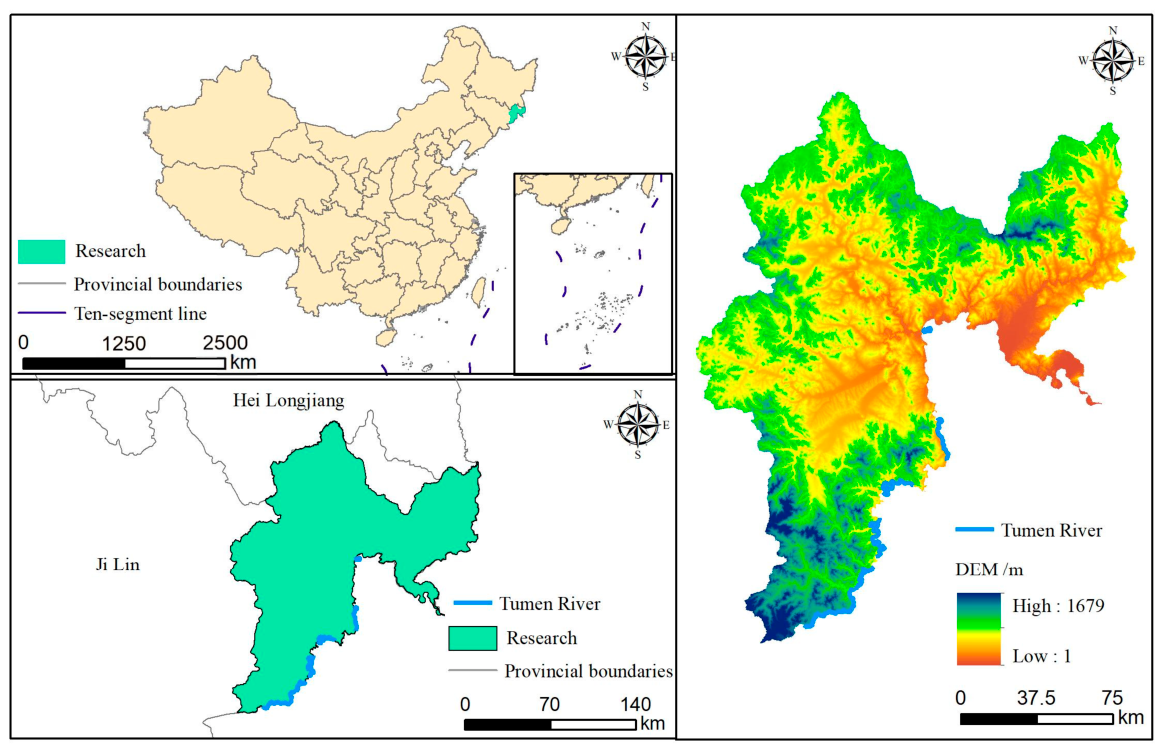
This study focuses on the Chinese portion of the Tumen River Basin, located in the Yanbian Korean Autonomous Prefecture in the southeastern Jilin Province and adjoining North Korea and Russia. Geographically, the study area spans 41°59′–44°30′ N and 127°27′–131°18′ E (Figure 1), with the modeled land-use area covering approximately 22,569 km². The river system is well developed, with the Tumen River as the main channel and the Hunchun, Gaya, Buerhatong, Hailan, Hongqi, and Mijiang Rivers as its major tributaries. The basin is generally humid and receives abundant precipitation. Seasonal differences are evident, with relatively dry conditions in spring and autumn and wetter conditions in summer and winter. The climate also exhibits pronounced vertical variation. During the warmest period from July to August, mean temperatures range from approximately 22 °C to 25 °C. Annual precipitation is approximately 400–800 mm and is jointly influenced by topographic and climatic factors [25]. Examining how land use and carbon storage have changed within the Chinese portion of the basin helps characterize regional ecological dynamics, provides a basis for sustainable land use and socioeconomic planning, and facilitates the evaluation of future carbon-storage trajectories.

2.2. Data Preparation and Sources

The Resource and Environmental Science and Data Center of the Chinese Academy of Sciences provided the 30 m land-use datasets used for 1990, 2000, 2010, and 2020. The land-use data were classified into six categories: Cropland, Forest, Grassland, Water, Built-up, and Unused. The land-use data and class-specific carbon-density parameters were used as inputs to the InVEST Carbon Storage and Sequestration model. The natural, socioeconomic, and accessibility variables listed in

Table 1. Spatial datasets and their corresponding sources.

Data Category	Data Name	Year(s)	Spatial Resolution (m)	Data Source
Basic data	Administrative boundary vector data of Yanbian Prefecture	2024	-	Public Geographic Information Service Platform
	Land-use data	1990, 2000, 2010 and 2020	30	Resource and Environmental Science and Data Center, Chinese Academy of Sciences (http://www.resdc.cn)
Natural data	Digital elevation model (DEM)	2020	30	Geospatial Data Cloud (https://www.gscloud.cn)
	Slope	2020	30	Derived from DEM data
	Aspect	2020	30	Derived from DEM data
	Mean annual temperature (TEM)	2020	1000	Resource and Environmental Science and Data Center, Chinese Academy of Sciences (http://www.resdc.cn)
	Annual precipitation (PRE)	2020	1000
	Normalized Difference Vegetation Index (NDVI)	2020	30
Socioeconomic data	Gross domestic product (GDP)	2020	1000	Resource and Environmental Science and Data Center, Chinese Academy of Sciences (http://www.resdc.cn)
	Population (POP)	2020	1000
	Nighttime light data (NLI)	1992–2021	500	Zenodo (https://zenodo.org/)
Accessibility data	Distance to railways	2020	30	OpenStreetMap (https://www.openstreetmap.org/)
	Distance to water	2020	30

were used in the PLUS simulation and the XGBoost–SHAP analysis of carbon-storage spatial heterogeneity in 2020. All spatial layers were projected to a common coordinate system and resampled to a consistent grid in ArcGIS (v10.8.2).

2.3. InVEST-Based Carbon-Storage Estimation

2.3.1. Implementation of the Carbon Storage and Sequestration Module

Developed collaboratively by Stanford University, The Nature Conservancy, and the World Wildlife Fund, the Integrated Valuation of Ecosystem Services and Tradeoffs (InVEST) suite provides an open-source framework for assessing ecosystem-service functions and values and informing ecosystem-management decisions [26]. Carbon storage was estimated with the Carbon Storage and Sequestration module implemented in InVEST version 3.14.2 [27]. Because PLUS was used to generate future land-use data separately for each scenario, the standard Carbon Storage and Sequestration module was applied rather than the REDD scenario module. For each land-use class, total carbon density was obtained by summing the four carbon pools as follows:

C = C_above + C_below + C_soil + C_dead

(1)

In Equation (1), C represents the total carbon density assigned to a land-use class, whereas C_above, C_below, C_soil, and C_dead correspond to the aboveground biomass, belowground biomass, soil organic carbon, and dead organic matter pools, respectively. Carbon-density values are reported in t·hm⁻².

2.3.2. Correction of Carbon Density Parameters

Class-specific carbon-density values were first derived from previous studies for the Tumen River Basin and nearby or ecologically comparable areas [24,28,29], and were subsequently adjusted to better reflect the climatic conditions of the study area. Following the climate-correction framework used in previous carbon-storage studies, precipitation and temperature were incorporated into the adjustment of soil organic carbon and biomass carbon density [30,31,32,33]. The precipitation-related relationship is based on Alam et al. [31], while the temperature-related relationships were referenced from Giardina and Ryan [32] and Chen et al. [33]. The correction equations are given below:

$$C_{SP}=3.396\times MAP+3999.1$$

(2)

$$C_{BP}=6.789\times e^{(0.0054\times MAP)}$$

(3)

$$C_{BT}=28\times MAT+398$$

(4)

$$K_{\mathrm{B}\mathrm{P}}={\displaystyle \frac{C_{\mathrm{B}\mathrm{P}}^1}{C_{\mathrm{B}\mathrm{P}}^2}}$$

(5)

$$K_{\mathrm{B}\mathrm{T}}={\displaystyle \frac{C_{\mathrm{B}\mathrm{T}}^1}{C_{\mathrm{B}\mathrm{T}}^2}}$$

(6)

$$K_{\mathrm{B}}=K_{\mathrm{B}\mathrm{P}}{K}_{\mathrm{B}\mathrm{T}}$$

(7)

$$K_S={\displaystyle \frac{C_{SP}^1}{C_{SP}^2}}$$

(8)

In Equations (2)–(8), C_SP represents soil organic carbon density derived from annual precipitation, while C_BP and C_BT represent biomass carbon density derived from annual precipitation and mean annual temperature, respectively; all three variables are expressed in kg/m². MAP and MAT refer to mean annual precipitation (mm) and mean annual temperature (°C). K_BP and K_BT are the precipitation- and temperature-based correction coefficients, whereas K_B and K_S are the correction factors applied to biomass and soil carbon density, respectively. The resulting four-pool carbon-density parameters are listed in

Table 2. Carbon density of different land-use types in the Tumen River Basin (t·hm⁻²).

Land-Use Type	Aboveground Biomass Carbon	Belowground Biomass Carbon	Soil Organic Carbon	Dead Organic Carbon
Cropland	5.18	1.04	89.9	0
Forest	18.34	80.85	107.48	2.25
Grassland	0.74	7.14	90.74	0.25
Water	3.95	9.54	163.25	0.79
Built-up	1.06	5.7	65.71	0.61
Unused	9.47	12.16	22.73	0

.

To evaluate their regional plausibility, the corrected carbon-density parameters were benchmarked against values reported for the Tumen River Basin and ecologically comparable parts of Northeast China [24,28,29]. The resulting values fell within the ranges documented in these studies, supporting their application in the subsequent carbon-storage calculations.

2.4. PLUS Model

2.4.1. Model Building and Running

Land-use changes between 2000 and 2010 were used to calibrate PLUS (v1.4) and estimate class-specific development probabilities. In the LEAS module, land-use expansion between 2000 and 2010 and the selected driving-factor layers were used as inputs, with the number of decision trees in the random forest set to 50, the sampling rate set to 0.01, training features set to 11, and parallel threads set to 20. LEAS generated probability surfaces for individual land-use classes and quantified the contribution of each driving factor to their observed expansion [34].

The probability surfaces generated by LEAS were then transferred to the CA based on the multi-type Random Seeds (CARS) module. A cellular-neighborhood range of 3 and 20 parallel threads were specified. Patch generation was controlled using a decay coefficient of 0.2, a diffusion coefficient of 0.1, and a maximum random-seed ratio of 0.01 to regulate expansion speed, spatial extent, and simulation stochasticity, respectively. Neighborhood weights were calculated from the 1990–2020 expansion record as the share of total expansion attributable to each land-use class. Values were bounded between 0 and 1, with higher values indicating a stronger neighborhood effect on class expansion. The resulting weights for the six land-use classes were 0.349, 0.383, 0.170, 0.019, 0.053, and 0.026, respectively [34].

2.4.2. Accuracy Validation of the PLUS Model

Historical raster land-use data were used in PLUS to estimate future land-use demand. PLUS operates through two main modules: the Land Expansion Analysis Strategy (LEAS) and CA based on multi-type Random Seeds (CARS) [34]. Future demand for each land-use class was estimated by combining PLUS with the Markov model [35]. The Markov relationship is expressed as follows:

S_(t+1) = P_i,jS_t

(9)

In Equation (9), S_t+1 denotes the land-use state at time t + 1, S_t denotes the initial land-use state at time t, and P_ij represents the transition probability from land-use class i to class j.

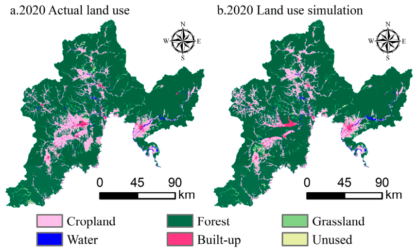
For retrospective validation, land-use changes between 2000 and 2010 were used to calibrate the land-expansion process, and the observed 2010 land-use map was used as the initial spatial state for simulating the 2020 land-use pattern. The simulated 2020 map was then compared with the observed 2020 land-use map. The comparison yielded a Kappa coefficient of 0.87 and an overall accuracy of 0.92, indicating satisfactory model performance for subsequent scenario simulations (Figure 2).

2.4.3. Multi-Scenario Simulation Settings

Three contrasting land-use pathways were specified for 2050: the Natural development, Ecological protection, and Urban development scenarios. Their comparison was intended to reveal how alternative land-use trajectories influence carbon storage and the balance between ecological conservation and regional development.

(1)

Natural development scenario

For the Natural development scenario, land-use demand in 2050 was extrapolated from the transition trends observed during 1990–2020, with no additional modification of inter-class transition probabilities. It therefore served as the reference pathway for evaluating the other two scenarios.

(2)

Ecological protection scenario

The Ecological protection scenario was formulated with reference to the conservation orientation of the Tumen City Territorial Spatial Master Plan (2021–2035) [36] and the Jilin Province Territorial Spatial Ecological Restoration Plan (2021–2035) [37]. Stronger restrictions on land-use conversion were applied to reduce anthropogenic disturbance to ecological land.

Compared with the Natural development scenario, conversion settings from Unused to Forest, Grassland, and Water were raised by 30%. In contrast, the settings for transitions from Cropland, Forest, and Grassland to Built-up were lowered by 20%; Cropland-to-Forest and Cropland-to-Grassland conversions were increased by 30% and 20%, respectively. National nature reserves and ecological protection areas were designated as restricted-development zones to maintain their integrity. Water areas were also designated as restricted-development zones under this scenario in consideration of their ecological value.

(3)

Urban development scenario

Drawing on the development orientation outlined in the Fourteenth Five-Year Plan for National Economic and Social Development and the Long-Range Objectives 2035 of Tumen City [38], the Urban development scenario depicts a pathway of intensified urbanization and industrial development. Accordingly, its transition settings favor the conversion of Unused and ecological land to Built-up while preventing Built-up from transitioning to other land-use classes. Relative to the Natural development scenario, the transition setting from Unused to Built-up increased by 30%; those from Forest, Grassland, and Water to Built-up increased by 20%; and the Cropland-to-Built-up setting increased by 30%. These settings were intended to represent stronger conversion toward Built-up under the Urban development scenario. National nature reserves remained designated as restricted-development zones.

The percentage adjustments specified for the Ecological protection and Urban development scenarios were treated as scenario parameters used to represent contrasting land-use pathways rather than as quantitative targets directly prescribed by the referenced planning documents.

2.5. Extreme Gradient Boosting (XGBoost)-Based Driving-Factor Analysis

2.5.1. Extreme Gradient Boosting (XGBoost)

Extreme Gradient Boosting (XGBoost) is a tree-based ensemble method within the gradient-boosting family [39]. Its predictive performance is improved by adding multiple weak learners sequentially. At each boosting step, a new tree is introduced to reduce the residual errors left by the preceding ensemble, and the final prediction is formed by combining the weighted outputs of all trees [40]. Although XGBoost generally provides strong predictive performance, its internal model structure remains difficult to interpret directly. To improve model interpretability, SHAP values were used to quantify the contribution of individual features to the model predictions. Grounded in cooperative game theory, SHAP assigns a theoretically consistent contribution value to each explanatory variable for a given model output. SHAP can be used for both global and local interpretation. For nonlinear tree models such as XGBoost, SHAP can further characterize interactions among variables and nonlinear threshold effects [41]. In contrast, traditional feature importance ranks or permutation importance methods usually struggle to provide a combined explanation of global contribution, local contribution, and nonlinear response mechanisms. Therefore, SHAP was employed to examine how individual explanatory variables contributed to the spatial variation in carbon storage in 2020. Using GeoDa (v1.22), global Moran’s I was calculated for the carbon-storage patterns in 1990, 2000, 2010, and 2020 to evaluate their spatial autocorrelation. The corresponding Moran’s I values were 0.756, 0.749, 0.742, and 0.735, respectively, and all were positive and statistically significant, indicating persistent positive spatial autocorrelation in carbon storage throughout the study period.

2.5.2. Model Training and Testing

Because XGBoost is relatively robust to multicollinearity among predictors, no preliminary screening of the driving variables was performed, thereby retaining the complete variable set for driver identification. Model development was conducted using Python (v3.11) in the JupyterLab environment. The 2020 carbon-storage samples from the Tumen River Basin were divided into training and test sets with an 8:2 ratio. Key XGBoost hyperparameters—including the number of trees, maximum depth, learning rate, subsampling ratio, and regularization terms—were tuned through Bayesian optimization. Five-fold cross-validation was embedded in the search procedure, with R² serving as the optimization criterion. The best-performing hyperparameter set was subsequently adopted to fit and validate the final model. The results showed that the model achieved R² values of 0.86 and 0.83 for the training and test sets of the Tumen River Basin, respectively, with relatively low RMSE, indicating strong predictive ability.

3. Results

3.1. Historical Changes in Land Use and Carbon Storage (1990–2020)

3.1.1. Evolution of Land-Use Patterns

The magnitude of change differed among land-use classes across the Tumen River Basin during 1990–2020. Overall, Forest remained relatively stable, Built-up expanded continuously, Cropland underwent localized restructuring, and Water increased.

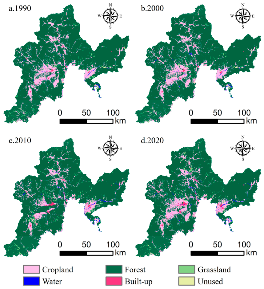
Among the different land-use types, Forest remained the dominant category throughout the study period and was relatively stable from 1990 to 2020. Cropland decreased slightly from 291.94 km² in 1990 to 276.99 km² in 2020, corresponding to an overall reduction of 14.95 km². Cropland occurred predominantly across river-valley plains and other low-lying terrain in the western and south-central basin, with its spatial distribution closely following the river network. Built-up showed the strongest expansion, rising from 18.98 km² in 1990 to 33.91 km² in 2020, equivalent to a 78.7% increase. Built-up expansion occurred mainly through the conversion of Cropland (18.90 km²) and Forest (2.18 km²), indicating continued encroachment of urban land on agricultural and ecological land. Spatially, Built-up was mainly concentrated in the south-central and southeastern parts of the basin. In 1990, Built-up was limited in scale and spatially fragmented. Its expansion accelerated during 2000–2010 and became more prominent by 2020, reflecting the continuous reshaping of the basin’s land-use pattern driven by urbanization. Water expanded from 6.94 km² in 1990 to 16.03 km² in 2020, a rise of 131%, representing the largest proportional increase among the six land-use classes. Grassland expanded from 36.34 km² in 1990 to 48.43 km² in 2020, adding 12.09 km² over the study period. Spatially, Grassland was scattered across the western and central mountain margins and the transition zones between Cropland and mountainous areas, with a relatively low degree of spatial aggregation. Unused increased from 4.52 km² in 1990 to 6.47 km² in 2020, showing only a limited magnitude of change. Its spatial distribution remained generally stable across the four periods, with no marked spatial variation (Figure 3).

3.1.2. Temporal Variation in Carbon Storage During 1990–2020

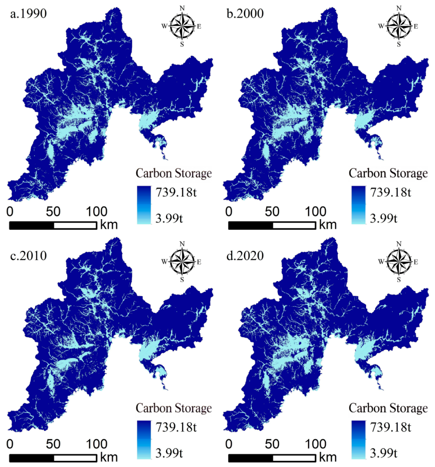
Figure 4 shows that carbon storage across the Tumen River Basin followed a staged pattern of “decline–recovery–decline” from 1990 to 2020, closely associated with the dynamic evolution of land-use patterns during the same period. At the basin scale, carbon storage was approximately 153.07 × 10⁸ t in 1990 and 152.98 × 10⁸ t in 2000. It subsequently rose to 155.78 × 10⁸ t in 2010 but fell to 151.03 × 10⁸ t by 2020, giving an overall reduction of approximately 1.33%.

Among the six land-use classes, Forest contained by far the largest carbon pool, representing more than 99% of basin-wide carbon storage in each of the four years. Consequently, variations in Forest largely determined the overall regional carbon pool. Forest carbon storage changed from 152.68 × 10⁸ t in 1990 to 150.62 × 10⁸ t in 2020, indicating a net decline over the study period. Spatially, high-carbon-storage areas consistently dominated the central-northern and western mountainous and hilly regions, showing a relatively stable spatial pattern. Carbon stored in Cropland decreased overall, from 31.20 × 10⁶ t in 1990 to 29.57 × 10⁶ t in 2020, resulting in a net loss of 1.63 × 10⁶ t. Spatially, Cropland was mainly concentrated in the western and south-central river valley plains of the basin. For Built-up, carbon storage rose from 1.53 × 10⁶ t in 1990 to 2.75 × 10⁶ t in 2020, representing an overall increase of 79.8%. However, the conversion of higher-carbon-density land-use classes to Built-up during its expansion contributed to losses in the basin-wide carbon pool. Spatially, as Built-up continued to expand along transportation corridors and both sides of rivers in the south-central and southeastern parts of the basin, low-carbon-storage areas became increasingly contiguous during 2010–2020. By 2020, low-carbon-storage areas in the south-central and southeastern basin were more spatially connected than in the other three periods. Over the 30-year period, carbon storage associated with Water rose by approximately 133%, the largest proportional change among the six land-use classes. This trend was highly consistent with the 131% expansion in Water area. However, because Water occupied only a small proportion of the basin, its contribution to the overall carbon-storage pattern remained limited. Grassland contributed a relatively small amount to total carbon storage and was spatially embedded as fragmented patches between Forest and Cropland. Unused contributed the least to total carbon storage and had only a minor effect on the basin-wide carbon-storage pattern.

3.2. Future Land-Use and Carbon-Storage Outcomes Under Multiple Scenarios

3.2.1. Spatiotemporal Changes in Land Use Under Different Scenarios from 2020 to 2050

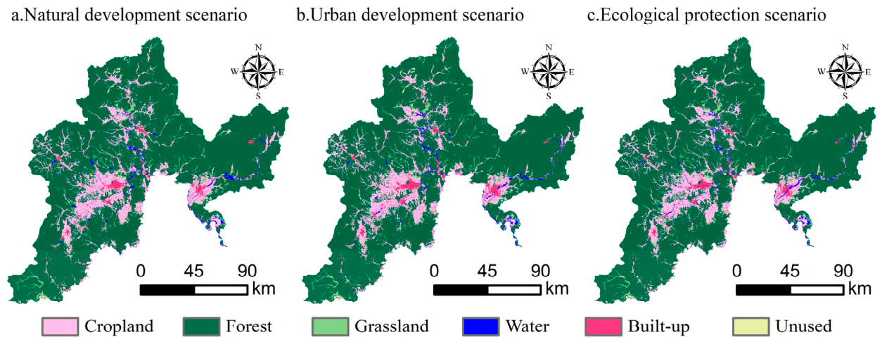
The simulated land-use patterns for 2050 showed that Forest remained the dominant land-use class under all three scenarios, with most of the Forest area distributed across mountain and hill zones in the central and northern parts of the basin. Nevertheless, the extent and spatial arrangement of Forest varied substantially among the scenarios.

Across the three scenarios, the Ecological protection scenario was the only scenario in which Forest achieved a net increase, with an expansion of 4.51 km², and a comparatively more continuous Forest pattern was observed. Under the Natural development scenario, Forest decreased by 189.35 km², accompanied by substantial changes in its spatial pattern. The Urban development scenario resulted in the largest Forest loss, with a net decrease of 203.62 km². More fragmented Forest patterns were observed in transition zones adjoining Forest, Cropland, and Built-up, particularly across the south-central and southeastern basin.

Cropland was concentrated in the western and south-central river valley plains under all three scenarios, and its belt-like distribution along rivers was largely maintained. Under the Ecological protection scenario, Cropland experienced the largest net decrease, declining by 150.77 km². The retreat of sloping Cropland and Cropland in ecologically sensitive areas was evident, and 137.61 km² of Cropland was converted to Forest. Under the Urban development scenario, Cropland decreased by approximately 72.05 km², mainly due to its conversion to Built-up, which reached 166.50 km². Spatially, Cropland patches in the western and south-central parts of the basin showed evident shrinkage. Under the Natural development scenario, Cropland decreased by approximately 25.89 km², and its spatial pattern was most similar to that in 2020.

Built-up increased by 44.2% under the Urban development scenario, with expansion concentrated along transportation corridors and both sides of rivers, where larger contiguous Built-up areas developed. The increase in Built-up was 99.99 km² under the Natural development scenario, compared with approximately 53.82 km² under the Ecological protection scenario, indicating a lower level of outward urban expansion in the latter. Grassland showed a slight net increase under all three scenarios and was scattered along the western mountain margins and the Cropland–Forest transition zones (

Table 3. Land-use area in 2050 under different scenarios (km²).

Land-Use Type	Cropland	Forest	Grassland	Water	Built-Up	Unused
2050 Natural development scenario	3050.72	18,149.99	560.34	257.44	476.85	73.52
2050 Urban development scenario	3004.56	18,135.72	557.12	255.30	543.33	72.82
2050 Ecological protection scenario	2925.84	18,343.85	559.98	238.16	430.68	70.34

). Its spatial aggregation remained low, and differences among scenarios were not pronounced.

3.2.2. Carbon-Storage Outcomes Under the 2050 Scenarios

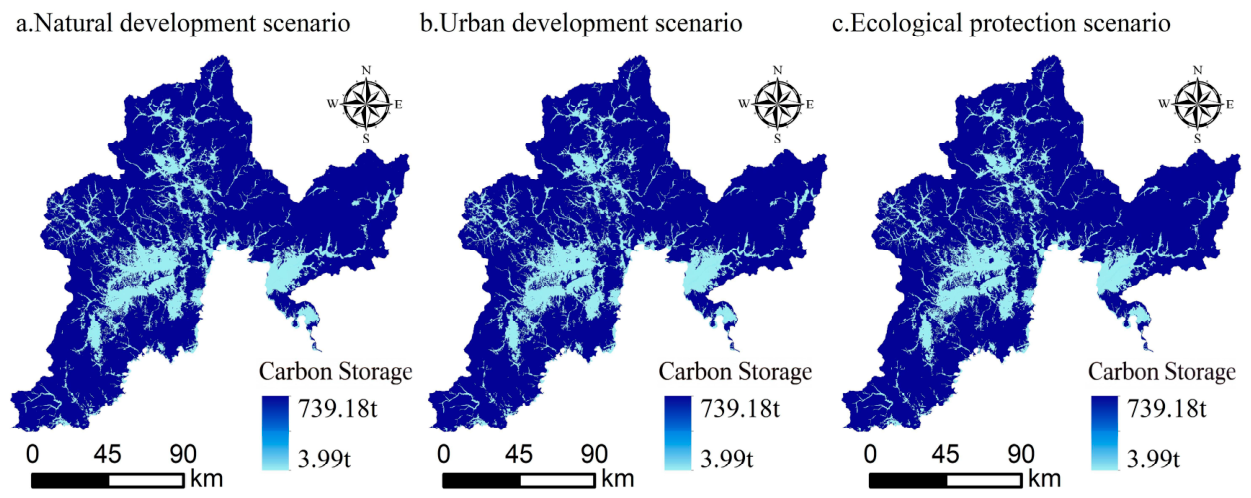
Carbon storage differed markedly among the three 2050 scenarios. These differences corresponded closely to scenario-specific changes in land use (Figure 5). Because Forest accounted for the overwhelming majority of the basin’s carbon storage, changes in the Forest carbon pool largely determined the direction and magnitude of the total carbon-storage response (Figure 6).

Only the Ecological protection scenario yielded a net increase in carbon storage. Total carbon storage reached approximately 151.07 × 10⁸ t in 2050, which was 3.82 × 10⁶ t higher than the 2020 level. Forest carbon storage increased by 3.70 × 10⁶ t, consistent with the 4.51 km² net gain in Forest area under this scenario. Built-up carbon storage increased by 3.93 × 10⁵ t; however, its 2050 value remained lower than under the other two scenarios, consistent with the comparatively limited expansion of Built-up under Ecological protection.

By 2050, total carbon storage in the Natural development scenario had fallen to approximately 149.50 × 10⁸ t, which was 153.50 × 10⁶ t below the 2020 level. Among all land-use types, Forest carbon storage decreased by 155.51 × 10⁶ t, which was consistent with the reduction of 189.35 km² in Forest area. The greatest reduction in carbon storage occurred under the Urban development scenario. Total carbon storage decreased to approximately 149.38 × 10⁸ t in 2050 (

Table 4. Carbon-storage estimates by land-use class for the three 2050 scenarios (×10⁶ t).

Land-Use Type	Cropland	Forest	Grassland	Water	Built-Up	Unused	Total Carbon Storage
2050 Natural development scenario	29.32	14,906.72	5.54	4.57	3.48	0.33	14,949.96
2050 Urban development scenario	28.88	14,894.99	5.51	4.53	3.97	0.32	14,938.20
2050 Ecological protection scenario	28.12	15,065.93	5.54	4.23	3.15	0.31	15,107.28

), corresponding to a reduction of approximately 165.26 × 10⁶ t relative to 2020. The decline in Forest carbon storage was also greatest under this pathway, corresponding to the 203.62 km² loss of Forest and the 44.2% expansion of Built-up.

In terms of spatial pattern, high-carbon-storage areas dominated under all three scenarios, corresponding mainly to the concentrated Forest areas in the central-northern and western mountainous regions of the basin. The overall spatial pattern remained relatively stable. Scenario differences were more evident in the extent and location of low-carbon-storage areas. Under Urban development, these areas were most extensive and appeared more spatially connected in the south-central and southeastern basin. As Built-up expanded along transportation corridors and both sides of rivers, areas of higher-carbon-density Forest were increasingly replaced by lower-carbon-density Built-up, and high-carbon-storage areas appeared more spatially fragmented. Low-carbon-storage areas expanded to a smaller extent under Natural development than under Urban development. The Ecological protection scenario showed the smallest extent of low-carbon-storage areas, while high-carbon-storage areas were best preserved and Forest patches exhibited the greatest continuity, resulting in the most effectively maintained carbon-storage pattern among the three scenarios.

3.3. Spatial Drivers of Carbon Storage in 2020

3.3.1. Importance Ranking of Explanatory Variables for Spatial Heterogeneity in Carbon Storage

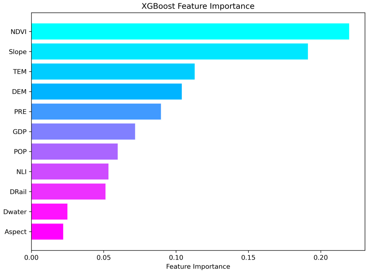
The XGBoost feature-importance results for 2020 quantified the relative contribution of each explanatory variable to the modeled spatial variation in carbon storage (Figure 7). NDVI ranked first among the selected variables, indicating that vegetation condition contributed most strongly to the XGBoost model’s differentiation of carbon-storage patterns. The high importance of NDVI was consistent with the dominant role of Forest in shaping the basin-wide carbon-storage pattern. Slope had the second-highest importance score. Its relatively high ranking reflects the close association between topographic conditions and the spatial differentiation of carbon storage. Mean annual temperature and elevation followed slope in importance. Temperature influences carbon storage by regulating photosynthesis and organic matter decomposition, whereas elevation affects carbon storage mainly by controlling the vertical distribution of vegetation zones. Annual precipitation ranked fifth, reflecting its role as a key water source for vegetation growth and ecosystem carbon accumulation. GDP and population contributed socioeconomic information to the model, although their global importance was lower than that of the leading natural variables. Their directional associations were examined further using SHAP values in the subsequent analysis. NLI and distance to railways served as proxy indicators of urbanization intensity and transportation accessibility, respectively. Distance to water and aspect ranked relatively low, indicating smaller global contributions to the XGBoost model than the higher-ranked variables.

3.3.2. Nonlinear Effects of Driving Factors on the Spatial Heterogeneity of Carbon Storage Based on the XGBoost–SHAP Model

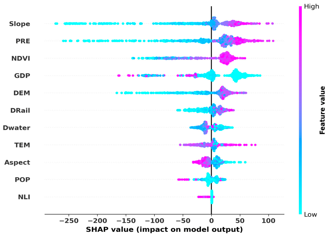
Figure 8 further reveals the direction and magnitude of the nonlinear effects of each driving factor on the spatial heterogeneity of carbon storage in the basin based on the SHAP values. Slope exhibited the widest range of SHAP values, indicating the greatest variation in model contribution across the analyzed samples. This finding is consistent with its second-place ranking in the XGBoost feature importance results. In low-slope areas, SHAP values were concentrated within strongly negative ranges. This is mainly because flat areas are generally occupied by Cropland and Built-up, where vegetation carbon density is relatively low, thereby exerting a strong negative effect on carbon storage. In contrast, SHAP values in high-slope mountainous areas were mostly positive, possibly because Forest is better preserved in these areas and carbon storage is relatively high.

The SHAP value distribution of precipitation was similar to that of slope. Low-precipitation areas showed strongly negative SHAP values, indicating a negative association between lower precipitation and the model-predicted carbon storage. In high-precipitation areas, SHAP values were mainly positive, indicating a positive model contribution at higher precipitation levels. Notably, the SHAP effect magnitude of precipitation was much larger than implied by its feature importance ranking, indicating that precipitation exhibited substantial sample-specific SHAP contributions despite its lower global feature-importance ranking. High-NDVI areas showed significant positive contributions, whereas low-NDVI areas exhibited clear negative effects. This pattern is highly consistent with the result that NDVI ranked first in feature importance, and its direction of influence was relatively clear. GDP showed an influence pattern that was markedly different from those of natural factors. High-GDP samples were predominantly associated with negative SHAP values, whereas low-GDP samples tended to show positive values. This contrast indicates a model-derived association between economic intensity and carbon storage and is consistent with a potential spatial tradeoff between socioeconomic development and carbon-storage conservation. The SHAP response pattern of elevation was highly similar to that of slope. Low-elevation plains and river valleys showed pronounced negative effects, whereas high-elevation areas made clear positive contributions. Together, slope and elevation exhibited similar topographic response patterns in the model. The positive and negative effects of temperature alternated across different temperature ranges, indicating that temperature exerted complex nonlinear effects on carbon storage by jointly regulating photosynthetic rates and organic matter decomposition. The overall effect magnitude of distance to railways was limited. Areas close to railways were more strongly affected by human disturbance and therefore showed slightly negative SHAP values. Aspect, population, and nighttime light index had SHAP values highly concentrated around zero, indicating that their nonlinear contributions to the spatial heterogeneity of carbon storage were relatively limited.

3.3.3. Threshold Effects of Driving Factors on the Spatial Heterogeneity of Carbon Storage Based on the XGBoost–SHAP Model

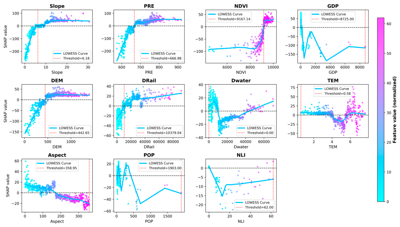
Based on SHAP dependence plots and locally weighted scatterplot smoothing (LOWESS) curves shown in Figure 9, model-derived threshold points were identified to characterize nonlinear changes in the associations between the explanatory variables and carbon storage. When slope was lower than 6.18°, SHAP values increased sharply with increasing slope, indicating that the strongly negative SHAP association observed at low slope values weakened rapidly as slope increased. Beyond this threshold, SHAP values tended to stabilize and remained slightly positive. The threshold response pattern of precipitation was similar to that of slope. When precipitation was below 666.98 mm, SHAP values increased rapidly, indicating that the strongly negative SHAP association at lower precipitation levels weakened as precipitation increased. Beyond this threshold, SHAP values tended to stabilize in the positive range. NDVI exhibited a typical nonlinear response characterized by “slow growth followed by a sharp increase”. Below the threshold, SHAP values remained in a low negative range for an extended interval, suggesting that the promotion effect of increasing vegetation cover on carbon storage was limited. When NDVI exceeded 0.92, SHAP values rose sharply into the positive range, indicating a substantial enhancement of the positive effect of high vegetation cover. Elevation was associated with negative SHAP values below 442.65 m. Above this threshold, SHAP values stabilized and became slightly positive. GDP exhibited a non-monotonic response, with a model-derived breakpoint at approximately CNY 8725. Above this value, SHAP values remained consistently negative, suggesting that the negative association between GDP and modeled carbon storage became relatively stable. This result is consistent with the predominantly negative SHAP values observed for high-GDP samples in the nonlinear response analysis. Distance to railways showed a model-derived breakpoint at approximately 10,379.04 m, representing the spatial influence boundary associated with transportation accessibility. Areas closer to railways generally exhibited negative SHAP values, whereas SHAP values shifted toward the positive range beyond this breakpoint, indicating a weaker negative association with transportation accessibility as distance increased. Distance to water revealed a localized positive effect of water availability on vegetation carbon accumulation near Water. Temperature showed an overall negative SHAP response, indicating a predominantly negative model association over the observed temperature range. The threshold effects of aspect, population, and nighttime light index were generally weak, which is consistent with the results of the feature importance and nonlinear response analyses.

4. Discussion

4.1. Interpretation of Spatial Carbon-Storage Heterogeneity in the Tumen River Basin

Based on XGBoost and SHAP analyses, this study interpreted the spatial heterogeneity of carbon storage in the Tumen River Basin from three perspectives: variable importance, nonlinear response patterns, and model-derived thresholds. The results showed that the spatial heterogeneity of carbon storage in the basin was associated with the combined influence of natural and socioeconomic factors. Among these factors, vegetation condition and topographic characteristics showed the strongest associations with carbon-storage spatial heterogeneity. Climatic factors also exhibited notable associations, and socioeconomic factors showed more localized effects mainly associated with land-use change.

Vegetation condition was identified as the leading explanatory factor associated with the spatial heterogeneity of carbon storage [42]. NDVI had the highest importance score, and its threshold effect further revealed a nonlinear response pattern characterized by “slow growth followed by a sharp increase”. When NDVI was below 0.92, SHAP values remained relatively low. Once NDVI exceeded this model-derived breakpoint, SHAP values increased sharply and shifted into the positive range, indicating a stronger positive model association between high vegetation cover and carbon storage. Because NDVI reflects vegetation condition and vigor, its variation can serve as an indicator of vegetation-related differences in ecosystem carbon storage [43]. This result accords with the predominant contribution of Forest to the basin-wide carbon-storage pattern and implies that sustaining dense vegetation cover is important for preserving the basin’s carbon-storage capacity [44]. Previous studies have also confirmed a significant positive nonlinear relationship between vegetation coverage and ecosystem carbon density, indicating that vegetation degradation may lead to a disproportionate decline in carbon storage [45].

Topographic conditions are important structural regulators of the spatial pattern of carbon storage [46]. In this study, slope showed the widest distribution of SHAP values, indicating the largest variation in model contribution among the selected variables. The threshold analysis showed that a slope of 6.18° represented a key topographic boundary for differentiating high and low carbon storage in the basin. Flat areas below this threshold were mainly occupied by Cropland and Built-up, which have relatively low carbon density and were therefore associated with strongly negative SHAP contributions. In contrast, hilly and mountainous areas above this threshold generally retained better-preserved Forest, and carbon storage tended to remain stable. The threshold response of elevation was broadly consistent with that of slope, suggesting a combined topographic influence on the modeled spatial variation in carbon storage. At higher elevations, land cover is increasingly dominated by natural ecosystems, which are generally associated with greater carbon storage; comparable patterns have also been reported in previous studies [47,48]. This pattern is consistent with the ecological mechanism by which complex terrain in mountainous basins limits human disturbance and helps preserve vegetation carbon pools. These findings suggest that topographic complexity plays an important role in shaping the spatial heterogeneity of carbon storage in the Tumen River Basin [49].

Climatic factors exert important regulatory effects on carbon storage through the spatial differentiation of hydrothermal conditions [50]. Previous research has not reached a uniform conclusion regarding the response of carbon storage to climate warming. Higher temperatures may promote carbon accumulation by enhancing plant productivity, but they may also accelerate carbon decomposition [51,52]. Precipitation effects are likewise context dependent: Wang et al. (2021) observed a positive carbon-storage–precipitation relationship in wetlands of the northeastern Tibetan Plateau [53], whereas Saiz et al. (2012) documented a negative linear response under different environmental settings [54]. The SHAP value distribution of precipitation was similar in width to that of slope, suggesting that its actual effect magnitude may have been underestimated by the feature importance metric. The SHAP dependence analysis identified a model-derived breakpoint at approximately 666.98 mm, below which precipitation was associated with strongly negative SHAP contributions. In areas below this threshold, vegetation growth may be constrained by water stress, which may be associated with lower carbon storage. Future changes in temperature and precipitation regimes may alter the spatial distribution of vegetation and carbon storage in the Tumen River Basin, introducing additional uncertainty into the basin’s carbon-storage pattern under climate change [25].

Socioeconomic variables showed weaker global importance than the leading natural variables but exhibited localized negative SHAP associations. Above the model-derived GDP breakpoint of CNY 8725, the corresponding SHAP contribution remained predominantly negative and relatively stable. This pattern is consistent with more intensive land development in economically active areas, where conversion of higher-carbon-density Forest to Built-up can reduce ecosystem carbon storage [55]. Distance to railways revealed the spatial influence boundary of transportation accessibility on carbon storage. This finding is consistent with previous studies showing that transportation infrastructure construction can enhance land accessibility, accelerate surrounding land development, and consequently lead to carbon storage loss [56]. Although population and NLI had relatively small global contributions, their predominantly negative SHAP values suggest that settlement and urban-development pressures may still be associated with localized carbon-storage losses [57].

Overall, the 2020 carbon-storage pattern was associated primarily with natural environmental gradients, while socioeconomic and accessibility variables contributed more localized effects. Natural factors were associated with the broad spatial framework of carbon storage through vegetation patterns, topographic conditions, and hydrothermal environments. Socioeconomic influences were associated with more localized modifications of this broader natural pattern, mainly through land-use conversion. Accordingly, key topographic breakpoints can be used to help identify priority areas for carbon-storage conservation in the basin. Meanwhile, the GDP breakpoint and the spatial influence boundary of transportation accessibility could be considered as supplementary information for land-development intensity regulation. This integrated approach can promote the coordinated protection of natural ecological conditions and the regulation of human activities, thereby providing scientific support for the long-term stability of the basin’s carbon storage function.

4.2. Implications for Sustainable Land-Use and Watershed Management

The findings of this study have direct implications for sustainable land-use and watershed management in the Tumen River Basin. The multi-scenario results demonstrate that development pathways generate substantially different carbon-storage outcomes. The Ecological protection scenario uniquely achieved a net gain in total carbon storage while maintaining greater spatial continuity of high-carbon Forest, whereas the largest decline occurred under the Urban development scenario. This contrast indicates that the sustainability of regional development depends not only on controlling the total area of Built-up land but also on regulating its spatial expansion into forested and ecologically sensitive areas.

The identified nonlinear thresholds provide additional guidance for spatially differentiated management. Areas characterized by low NDVI, gentle slopes, low elevations, insufficient precipitation, high economic activity, or strong transportation accessibility were generally associated with lower carbon storage and may therefore warrant priority consideration in land-development control, ecological restoration, and vegetation improvement. In contrast, mountainous Forest areas with high vegetation coverage could be prioritized as core areas for carbon-storage conservation. Incorporating these spatial thresholds into territorial spatial planning could improve the precision of ecological zoning and reduce conflicts between economic development and ecosystem conservation.

From a broader sustainability perspective, the combined analytical framework using InVEST, PLUS, XGBoost, and SHAP links ecosystem-service assessment, future scenario analysis, and interpretable machine learning. It therefore provides a potentially transferable approach for evaluating tradeoffs among urbanization, ecological protection, and carbon-storage conservation in other ecologically sensitive and transboundary river basins.

4.3. Limitations and Future Research

Several limitations should be considered when interpreting the results. First, the InVEST Carbon Storage and Sequestration Module estimates carbon storage using land-use classes and class-specific carbon-density parameters. Consequently, the adopted approach does not explicitly represent within-class differences in vegetation condition or the spatial variability of carbon density within the same land-use class. Second, the carbon-density parameters used in this study were mainly derived from published studies and adjusted using climatic relationships. Although these corrections improve regional applicability, uncertainty in the underlying parameters is inevitably propagated into the carbon-storage estimates. The analysis also assumes that the class-specific carbon-density parameters remained constant over the study period and across future scenarios. Third, the 2050 PLUS simulations represent conditional land-use scenarios based on historical transitions and specified scenario settings rather than deterministic forecasts of future land use. Fourth, the random train–test partition used in the XGBoost analysis did not explicitly account for spatial dependence among neighboring samples. Given the significant positive spatial autocorrelation in carbon storage, the reported predictive performance may therefore be somewhat optimistic, and spatial block cross-validation would provide a more rigorous assessment of spatial generalizability. Fifth, the response variable used in the XGBoost–SHAP analysis was the 2020 carbon-storage raster estimated by InVEST from land-use classes and class-specific carbon-density parameters. Consequently, the SHAP results partly reflect the spatial structure embedded in the InVEST-derived carbon-storage pattern and should be interpreted as associations with modeled carbon storage rather than as independent causal effects on observed ecosystem carbon density. Future research should incorporate field-measured and spatially explicit carbon-density data, dynamic carbon-density parameters, higher-resolution remote-sensing information, independent carbon-storage observations, spatial block cross-validation, and process-based ecological models to improve carbon-storage estimation and provide a stronger process-based understanding of the observed spatial patterns.

5. Conclusions

This study used InVEST and PLUS to assess historical carbon-storage changes and future land-use scenarios in the Tumen River Basin, while XGBoost–SHAP was applied separately to the 2020 spatial data to interpret carbon-storage spatial heterogeneity. From 1990 to 2020, Forest remained the dominant land-use class and the primary contributor to carbon storage, whereas Built-up expanded continuously. Total carbon storage followed a decline–recovery–decline trajectory, decreasing from 153.07 × 10⁸ t in 1990 to approximately 151.03 × 10⁸ t in 2020. The expansion of Built-up and the reduction in Forest were closely associated with carbon-storage losses during the study period.

The 2050 scenario simulations revealed clear differences among alternative land-use pathways. The Ecological protection scenario was the only scenario that produced a net increase in total carbon storage relative to 2020 (+3.82 × 10⁶ t), whereas the Urban development scenario resulted in the largest loss (−165.26 × 10⁶ t). These results indicate that maintaining Forest continuity and limiting the conversion of carbon-dense land to Built-up are important for sustaining the basin’s carbon-storage function. More broadly, the comparison among scenarios highlights the need to balance ecological conservation, land development, and carbon-storage protection in sustainable land-use and watershed management.

For the 2020 spatial pattern, XGBoost–SHAP identified NDVI and slope as the leading explanatory variables and revealed nonlinear associations involving climatic, topographic, socioeconomic, and accessibility variables. Model-derived breakpoints were identified for slope (6.18°), precipitation (666.98 mm), NDVI (0.92), elevation (442.65 m), GDP (CNY 8725), and distance to railways (10,379.04 m). These thresholds can serve as supplementary spatial information for differentiated land-use management rather than as fixed regulatory boundaries. Several limitations should also be recognized: the InVEST estimates depend on class-specific carbon-density parameters and do not fully represent within-class spatial variability; the PLUS results are conditional scenarios rather than deterministic forecasts; and XGBoost–SHAP identifies associations and response patterns but does not establish causal relationships. Future research should incorporate field-measured and spatially explicit carbon-density data, dynamic carbon-density parameters, higher-resolution remote-sensing information, and process-based ecological models to improve carbon-storage estimation and strengthen the process-based understanding of observed spatial patterns.

References

1. Brown, P.T.; Hanley, H.; Mahesh, A.; Reed, C.; Strenfel, S.J.; Davis, S.J.; Kochanski, A.K.; Clements, C.B. Climate warming increases extreme daily wildfire growth risk in California. Nature 2023, 621, 760–766. [Google Scholar] [CrossRef] [Scilit] [PubMed]
2. Piao, S.; Fang, J.; Ciais, P.; Peylin, P.; Huang, Y.; Sitch, S.; Wang, T. The carbon balance of terrestrial ecosystems in China. Nature 2009, 458, 1009–1013. [Google Scholar] [CrossRef] [Scilit] [PubMed]
3. Ghosh, S.; Dinda, S.; Das Chatterjee, N.; Dutta, S.; Bera, D. Spatial-explicit carbon emission-sequestration balance estimation and evaluation of emission susceptible zones in an Eastern Himalayan city using Pressure-Sensitivity-Resilience framework: An approach towards achieving low carbon cities. J. Clean. Prod. 2022, 336, 130417. [Google Scholar] [CrossRef] [Scilit]
4. Huang, W.; Guo, L.; Zhang, T.; Chen, T.; Chen, L.; Li, L.; Zhang, X. The impact of territorial spatial transformation on carbon storage: A case study of Suqian, East China. Land 2024, 13, 348. [Google Scholar] [CrossRef] [Scilit]
5. Xiang, S.; Wang, Y.; Deng, H.; Yang, C.; Wang, Z.; Gao, M. Response and multi-scenario prediction of carbon storage to land use/cover change in the main urban area of Chongqing, China. Ecol. Indic. 2022, 142, 109205. [Google Scholar] [CrossRef] [Scilit]
6. Lewis, C.J.E.; Baldock, J.A.; Hawke, B.; Gadd, P.S.; Zawadzki, A.; Heijnis, H.; Jacobsen, G.E.; Rogers, K.; Macreadie, P.I. Impacts of land reclamation on tidal marsh ‘blue carbon’ stocks. Sci. Total Environ. 2019, 672, 427–437. [Google Scholar] [CrossRef] [Scilit] [PubMed]
7. Yuan, N.; Wang, E.; Lv, S.; Tang, X.; Wang, T.; Wang, G.; Zhou, Y.; Zhou, G.; Shi, Y.; Xu, L. Degradation reduces greenhouse gas emissions while weakening ecosystem carbon sequestration of Moso bamboo forests. Sci. Total Environ. 2023, 877, 162915. [Google Scholar] [CrossRef] [Scilit] [PubMed]
8. Kohestani, N.; Rastgar, S.; Heydari, G.; Jouibary, S.S.; Amirnejad, H. Spatiotemporal modeling of the value of carbon sequestration under changing land use/land cover using InVEST model: A case study of Nour-rud Watershed, Northern Iran. Environ. Dev. Sustain. 2024, 26, 14477–14505. [Google Scholar] [CrossRef] [Scilit]
9. Li, J.; Gong, J.; Guldmann, J.-M.; Li, S.; Zhu, J. Carbon dynamics in the Northeastern Qinghai-Tibetan Plateau from 1990 to 2030 using Landsat land use/cover change data. Remote Sens. 2020, 12, 528. [Google Scholar] [CrossRef] [Scilit]
10. Yang, H.; Qin, Z.; Shu, Q.; Xi, L.; Xia, C.; Wu, Z.; Wang, M.; Duan, D. Estimation of the aboveground carbon storage of Dendrocalamus giganteus based on spaceborne lidar co-kriging. Forests 2024, 15, 1440. [Google Scholar] [CrossRef] [Scilit]
11. Wang, R.-Y.; Cai, H.; Chen, L.; Li, T. Spatiotemporal evolution and multi-scenario prediction of carbon storage in the GBA based on PLUS-InVEST models. Sustainability 2023, 15, 8421. [Google Scholar] [CrossRef] [Scilit]
12. Wu, B.; Garcia Maya, B.I.; Limnios, N. Using semi-Markov chains to solve semi-Markov processes. Methodol. Comput. Appl. Probab. 2021, 23, 1419–1431. [Google Scholar] [CrossRef] [Scilit]
13. Dong, Z.R.; Yuan, Q.Z.; Wang, Z.C.; Ren, P. Analysis and simulation prediction of the evolutionary characteristics of living–production–ecological spatial conflicts in the agriculture–pastoral ecotone of western Sichuan: A case study of four counties in Aba Prefecture. Acta Ecol. Sin. 2023, 43, 6243–6256. (In Chinese) [Google Scholar]
14. Liu, X.; Liang, X.; Li, X.; Xu, X.; Ou, J.; Chen, Y.; Li, S.; Wang, S.; Pei, F. A future land use simulation model (FLUS) for simulating multiple land use scenarios by coupling human and natural effects. Landsc. Urban Plan. 2017, 168, 94–116. [Google Scholar] [CrossRef] [Scilit]
15. Fan, L.; Cai, T.; Wen, Q.; Han, J.; Wang, S.; Wang, J.; Yin, C. Scenario simulation of land use change and carbon storage response in Henan Province, China: 1990–2050. Ecol. Indic. 2023, 154, 110660. [Google Scholar] [CrossRef] [Scilit]
16. Xu, J.; Mu, X.; Ma, Z. Evaluation of the effectiveness of regulatory measures for the use of natural ecological space based on the remote sensing-driven PLUS-InVEST model: A case study from the Central Mountainous Area of Hainan Island. Ecol. Evol. 2025, 15, e72025. [Google Scholar] [CrossRef] [Scilit] [PubMed]
17. Kafy, A.; Saha, M.; Fattah, M.A.; Rahman, M.T.; Duti, B.M.; Rahaman, Z.A.; Bakshi, A.; Kalaivani, S.; Rahaman, S.N.; Sattar, G.S. Integrating forest cover change and carbon storage dynamics: Leveraging Google Earth Engine and InVEST model to inform conservation in hilly regions. Ecol. Indic. 2023, 152, 110374. [Google Scholar] [CrossRef] [Scilit]
18. Wang, C.Y.; Li, T.Z.; Guo, X.H.; Xia, L.; Lu, C.; Wang, C. PLUS-InVEST study of the Chengdu-Chongqing urban agglomeration’s land-use change and carbon storage. Land 2022, 11, 1617. [Google Scholar] [CrossRef] [Scilit]
19. Zhao, H.P.; Guo, B.; Wang, G.J. Spatial–temporal changes and prediction of carbon storage in the Tibetan Plateau based on PLUS-InVEST model. Forests 2023, 14, 1352. [Google Scholar] [CrossRef] [Scilit]
20. Li, Y.; Qiu, J.; Li, Z.; Li, Y. Assessment of blue carbon storage loss in coastal wetlands under rapid reclamation. Sustainability 2018, 10, 2818. [Google Scholar] [CrossRef] [Scilit]
21. Wang, S.; Peng, H. Multiple spatio-temporal scale runoff forecasting and driving mechanism exploration by K-means optimized XGBoost and SHAP. J. Hydrol. 2024, 630, 130650. [Google Scholar] [CrossRef] [Scilit]
22. Hao, L.; He, S.; Zhou, J.; Zhao, Q.; Lu, X. Prediction of the landscape pattern of the Yancheng Coastal Wetland, China, based on XGBoost and the MCE-CA-Markov model. Ecol. Indic. 2022, 145, 109735. [Google Scholar] [CrossRef] [Scilit]
23. Zhang, Y.; Jin, R.; Zhu, W.; Zhang, D.; Zhang, X. Impacts of land use changes on wetland ecosystem services in the Tumen River Basin. Sustainability 2020, 12, 9821. [Google Scholar] [CrossRef] [Scilit]
24. Xiang, H.; Jia, M.; Wang, Z.; Li, L.; Mao, D.; Zhang, D.; Cui, G.; Zhu, W. Impacts of land cover changes on ecosystem carbon stocks over the transboundary Tumen River Basin in Northeast Asia. Chin. Geogr. Sci. 2018, 28, 973–985. [Google Scholar] [CrossRef] [Scilit]
25. Ding, N.; Piao, D.; Cui, G.; Jeon, S. The impacts of climate variation and land use/cover change on net primary productivity in the Tumen River Basin. Landsc. Ecol. Eng. 2022, 18, 157–170. [Google Scholar] [CrossRef] [Scilit]
26. Mukhopadhyay, A.; Hati, J.P.; Acharyya, R.; Pal, I.; Tuladhar, N.; Habel, M. Global trends in using the InVEST model suite and related research: A systematic review. Ecohydrol. Hydrobiol. 2025, 25, 389–405. [Google Scholar] [CrossRef] [Scilit]
27. Natural Capital Project. InVEST: Integrated Valuation of Ecosystem Services and Tradeoffs, Version 3.14.2. Available online: https://invest.readthedocs.io/en/3.14.2/ (accessed on 11 August 2026).
28. Wang, Y.; Li, M.; Jin, G. Exploring the optimization of spatial patterns for carbon sequestration services based on multi-scenario land use/cover changes in the Changchun–Jilin–Tumen region, China. J. Clean. Prod. 2024, 438, 140788. [Google Scholar] [CrossRef] [Scilit]
29. Li, Y.; Liu, Z.; Li, S.; Li, X. Multi-scenario simulation analysis of land use and carbon storage changes in Changchun City based on FLUS and InVEST model. Land 2022, 11, 647. [Google Scholar] [CrossRef] [Scilit]
30. Raich, J.W.; Nadelhoffer, K.J. Belowground carbon allocation in forest ecosystems: Global trends. Ecology 1989, 70, 1346–1354. [Google Scholar] [CrossRef] [Scilit]
31. Alam, S.A.; Starr, M.; Clark, B.J.F. Tree biomass and soil organic carbon densities across the Sudanese woodland savannah: A regional carbon sequestration study. J. Arid Environ. 2013, 89, 67–76. [Google Scholar] [CrossRef] [Scilit]
32. Giardina, C.P.; Ryan, M.G. Evidence that decomposition rates of organic carbon in mineral soil do not vary with temperature. Nature 2000, 404, 858–861. [Google Scholar] [CrossRef] [Scilit] [PubMed]
33. Chen, G.S.; Yang, Y.S.; Liu, L.Z.; Li, X.B.; Zhao, Y.C.; Yuan, Y.D. Research progress on total belowground carbon allocation in forest ecosystems. J. Subtrop. Resour. Environ. 2007, 2, 34–42. (In Chinese) [Google Scholar] [CrossRef]
34. Gao, L.; Tao, F.; Liu, R.; Wang, Z.; Leng, H.; Zhou, T. Multi-scenario simulation and ecological risk analysis of land use based on the PLUS model: A case study of Nanjing. Sustain. Cities Soc. 2022, 85, 104055. [Google Scholar] [CrossRef] [Scilit]
35. Mo, J.; Sun, P.; Shen, D.; Li, N.; Zhang, J.; Wang, K. Simulation analysis of land-use spatial conflict in a geopark based on the GMOP-Markov-PLUS model: A case study of Yimengshan Geopark, China. Land 2023, 12, 1291. [Google Scholar] [CrossRef] [Scilit]
36. Jilin Provincial People’s Government. Reply on the Territorial Spatial Master Plans (2021–2035) of Yanji, Hunchun, Tumen, Dunhua, Longjing, Helong, Wangqing County, and Antu County; Ji Zheng Han [2024] No. 54; Jilin Provincial People’s Government: Changchun, China, 2024. (In Chinese)
37. Jilin Provincial Department of Natural Resources. Jilin Province Territorial Spatial Ecological Restoration Plan (2021–2035), Revised Edition; Jilin Provincial Department of Natural Resources: Changchun, China, 2024. (In Chinese)
38. Tumen Municipal People’s Government. Outline of the Fourteenth Five-Year Plan for National Economic and Social Development and the Long-Range Objectives for 2035 of Tumen City; Tumen Municipal People’s Government: Tumen, China, 2021. (In Chinese)
39. Dong, J.; Chen, Y.; Yao, B.; Zhang, X.; Zeng, N. A neural network boosting regression model based on XGBoost. Appl. Soft Comput. 2022, 125, 109067. [Google Scholar] [CrossRef] [Scilit]
40. Osman, A.I.A.; Ahmed, A.N.; Chow, M.F.; Huang, Y.F.; El-Shafie, A. Extreme gradient boosting (XGBoost) model to predict the groundwater levels in Selangor, Malaysia. Ain Shams Eng. J. 2021, 12, 1545–1556. [Google Scholar] [CrossRef] [Scilit]
41. Lundberg, S.M.; Erion, G.; Chen, H.; DeGrave, A.; Prutkin, J.M.; Nair, B.; Katz, R.; Himmelfarb, J.; Bansal, N.; Lee, S.-I. From local explanations to global understanding with explainable AI for trees. Nat. Mach. Intell. 2020, 2, 56–67. [Google Scholar] [CrossRef] [Scilit] [PubMed]
42. Nie, Q.; Wu, G.; Li, L.; Man, W.; Ma, J.; Bao, Z.; Luo, L.; Li, H. Exploring scaling differences and spatial heterogeneity in drivers of carbon storage changes: A comprehensive geographic analysis framework. Ecol. Indic. 2024, 165, 112193. [Google Scholar] [CrossRef] [Scilit]
43. Feng, H.; Kang, P.; Deng, Z.; Zhao, W.; Hua, M.; Zhu, X.; Wang, Z. The impact of climate change and human activities to vegetation carbon sequestration variation in Sichuan and Chongqing. Environ. Res. 2023, 238, 117138. [Google Scholar] [CrossRef] [Scilit]
44. Wei, X.; Yang, J.; Luo, P.; Lin, L.; Lin, K.; Guan, J. Assessment of the variation and influencing factors of vegetation NPP and carbon sink capacity under different natural conditions. Ecol. Indic. 2022, 138, 108834. [Google Scholar] [CrossRef] [Scilit]
45. Chen, Z.; Yu, G.; Ge, J.; Wang, Q.; Zhu, X.; Xu, Z. Roles of climate, vegetation and soil in regulating the spatial variations in ecosystem carbon dioxide fluxes in the Northern Hemisphere. PLoS ONE 2015, 10, e0125265. [Google Scholar] [CrossRef] [Scilit] [PubMed]
46. Zhu, M.; Feng, Q.; Qin, Y.; Cao, J.; Zhang, M.; Liu, W.; Deo, R.C.; Zhang, C.; Li, R.; Li, B. The role of topography in shaping the spatial patterns of soil organic carbon. CATENA 2019, 176, 296–305. [Google Scholar] [CrossRef] [Scilit]
47. Pouyat, R.V.; Yesilonis, I.D.; Nowak, D.J. Carbon storage by urban soils in the United States. J. Environ. Qual. 2006, 35, 1566–1575. [Google Scholar] [CrossRef] [Scilit] [PubMed]
48. Román-Sánchez, A.; Vanwalleghem, T.; Peña, A.; Laguna, A.; Giráldez, J.V. Controls on soil carbon storage from topography and vegetation in a rocky, semi-arid landscapes. Geoderma 2018, 311, 159–166. [Google Scholar] [CrossRef] [Scilit]
49. He, Y.; Bond-Lamberty, B.; Myers-Pigg, A.N.; Newcomer, M.E.; Ladau, J.; Holmquist, J.R.; Brown, J.B.; Falco, N. Effects of spatial variability in vegetation phenology, climate, landcover, biodiversity, topography, and soil property on soil respiration across a coastal ecosystem. Heliyon 2024, 10, e30470. [Google Scholar] [CrossRef] [Scilit] [PubMed]
50. Rodrigues, C.I.D.; Brito, L.M.; Nunes, L.J.R. Soil carbon sequestration in the context of climate change mitigation: A review. Soil Syst. 2023, 7, 64. [Google Scholar] [CrossRef] [Scilit]
51. Cao, M.; Woodward, F.I. Net primary and ecosystem production and carbon stocks of terrestrial ecosystems and their responses to climate change. Glob. Change Biol. 1998, 4, 185–198. [Google Scholar] [CrossRef] [Scilit]
52. Álvaro-Fuentes, J.; Easter, M.; Paustian, K. Climate change effects on organic carbon storage in agricultural soils of northeastern Spain. Agric. Ecosyst. Environ. 2012, 155, 87–94. [Google Scholar] [CrossRef] [Scilit]
53. Wang, Y.; Shen, X.; Jiang, M.; Tong, S.; Lu, X. Spatiotemporal change of aboveground biomass and its response to climate change in marshes of the Tibetan Plateau. Int. J. Appl. Earth Obs. Geoinf. 2021, 102, 102385. [Google Scholar] [CrossRef] [Scilit]
54. Saiz, G.; Bird, M.I.; Domingues, T.; Schrodt, F.; Schwarz, M.; Feldpausch, T.R.; Veenendaal, E.; Djagbletey, G.; Hien, F.; Compaore, H.; et al. Variation in soil carbon stocks and their determinants across a precipitation gradient in West Africa. Glob. Change Biol. 2012, 18, 1670–1683. [Google Scholar] [CrossRef] [Scilit]
55. Zhao, L.; Xin, W.; Mao, X.; Shao, D.; Chen, Q.; Zhu, Y.; Han, F. Trade-off relationships of ecosystem services for soil retention carbon sinks in the Loess Plateau of China. Land Use Policy 2025, 158, 107751. [Google Scholar] [CrossRef] [Scilit]
56. He, Y.; Liu, X.; Wu, D.; Li, S.; Zhou, P. Ecological risks and patterns associated with land use/cover changes along the Belt and Road Initiative routes. Land Degrad. Dev. 2025, 36, 2075–2094. [Google Scholar] [CrossRef] [Scilit]
57. Wang, X.; Zhang, W.; Zhao, X.; Wang, D.; Li, Y. Sustaining carbon storage: An analysis of land use and conservation strategies in China’s Huang-Huai-Hai Plain. Sustainability 2025, 17, 139. [Google Scholar] [CrossRef] [Scilit]
Figure 1. Location and topographic setting of the Tumen River Basin.
Sustainability 18 08555 g001
Figure 2. Comparison of simulated and observed land-use patterns in 2020.
Sustainability 18 08555 g002
Figure 3. Land-use distribution in the Tumen River Basin in 1990, 2000, 2010, and 2020.
Sustainability 18 08555 g003
Figure 4. Spatial distribution of carbon storage in the Tumen River Basin from 1990 to 2020.
Sustainability 18 08555 g004
Figure 5. Spatial distribution of land-use types under different scenarios in 2050.
Sustainability 18 08555 g005
Figure 6. Spatial distribution of carbon storage in the Tumen River Basin under different scenarios in 2050.
Sustainability 18 08555 g006
Figure 7. Relative importance of explanatory variables for carbon-storage spatial heterogeneity in 2020 based on XGBoost.
Sustainability 18 08555 g007
Figure 8. Nonlinear SHAP responses of explanatory variables associated with carbon-storage spatial heterogeneity in 2020.
Sustainability 18 08555 g008
Figure 9. Model-derived threshold responses of explanatory variables associated with carbon-storage spatial heterogeneity in 2020.
Sustainability 18 08555 g009